Efficient Algorithms for Ortho-Radial Graph Drawing

Abstract

Orthogonal drawings, i.e., embeddings of graphs into grids, are a classic topic in Graph Drawing. Often the goal is to find a drawing that minimizes the number of bends on the edges. A key ingredient for bend minimization algorithms is the existence of an orthogonal representation that allows to describe such drawings purely combinatorially by only listing the angles between the edges around each vertex and the directions of bends on the edges, but neglecting any kind of geometric information such as vertex coordinates or edge lengths.

Barth et al. [2] have established the existence of an analogous ortho-radial representation for ortho-radial drawings, which are embeddings into an ortho-radial grid, whose gridlines are concentric circles around the origin and straight-line spokes emanating from the origin but excluding the origin itself. While any orthogonal representation admits an orthogonal drawing, it is the circularity of the ortho-radial grid that makes the problem of characterizing valid ortho-radial representations all the more complex and interesting. Barth et al. prove such a characterization. However, the proof is existential and does not provide an efficient algorithm for testing whether a given ortho-radial representation is valid, let alone actually obtaining a drawing from an ortho-radial representation.

In this paper we give quadratic-time algorithms for both of these tasks. They are based on a suitably constrained left-first DFS in planar graphs and several new insights on ortho-radial representations. Our validity check requires quadratic time, and a naive application of it would yield a quartic algorithm for constructing a drawing from a valid ortho-radial representation. Using further structural insights we speed up the drawing algorithm to quadratic running time.

1 Introduction

Grid drawings of graphs embed graphs into grids such that vertices map to grid points and edges map to internally disjoint curves on the grid lines that connect their endpoints. Orthogonal grids, whose grid lines are horizontal and vertical lines, are popular and widely used in graph drawing. Among others, orthogonal graph drawings are applied in VLSI design (e.g., [30, 6]), diagrams (e.g., [4, 19, 14, 32]), and network layouts (e.g., [26, 23]). They have been extensively studied with respect to their construction and properties (e.g., [29, 7, 8, 25, 1]). Moreover, they have been generalized to arbitrary planar graphs with degree higher than four (e.g., [28, 18, 9]).

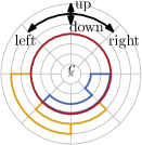
(a) Ortho-radial grid.

(b) Cylinder drawing.

Figure 1: An ortho-radial drawing of a graph on a grid (1(a)) and its equivalent interpretation as an orthogonal drawing on a cylinder (1(b)).

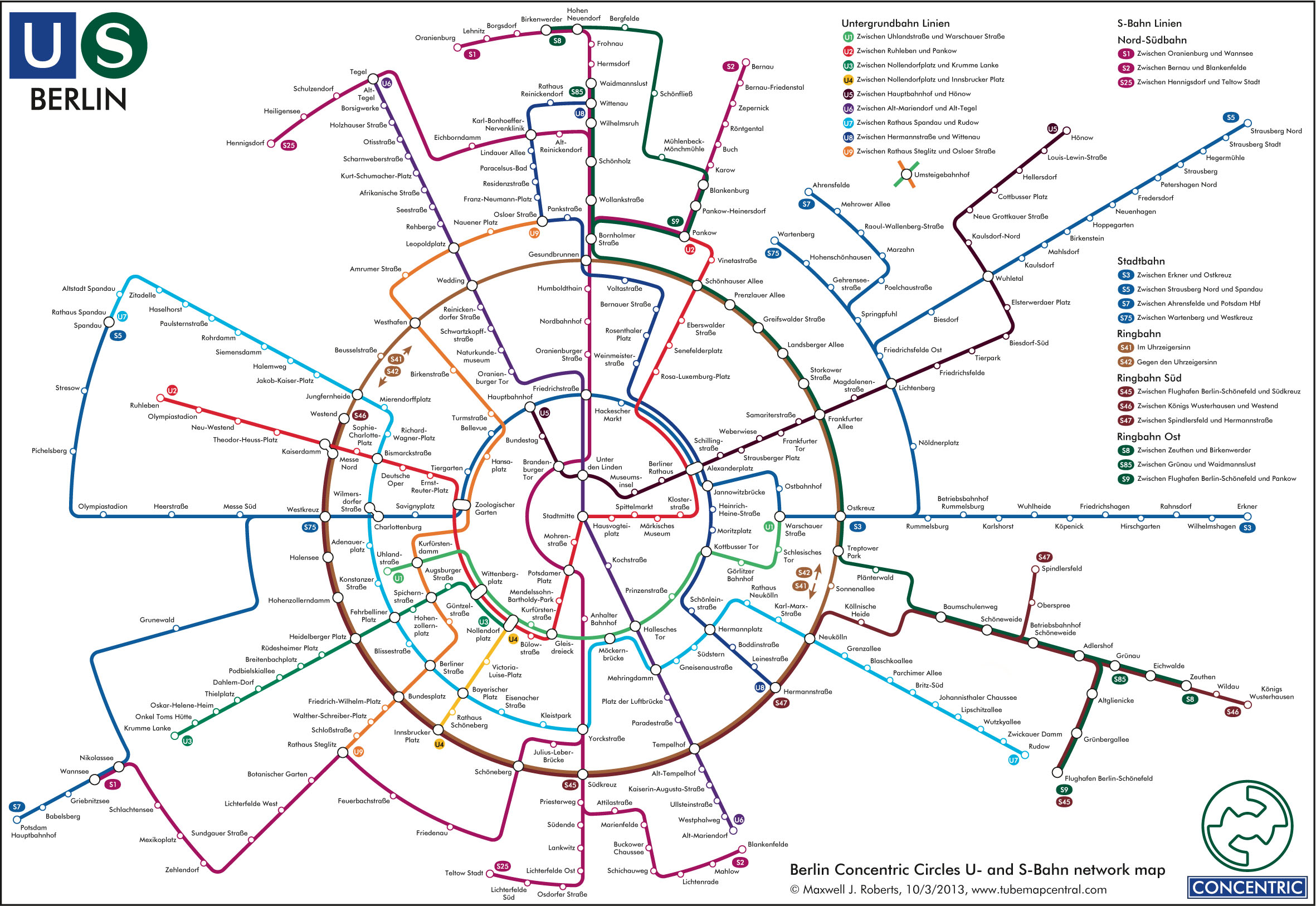
Figure 2: Metro map of Berlin using an ortho-radial layout. Image copyright by Maxwell J. Roberts. Reproduced with permission.

Ortho-radial drawings are a generalization of orthogonal drawings to grids that are formed by concentric circles and straight-line spokes from the center but excluding the center. Equivalently, they can be viewed as graphs drawn in an orthogonal fashion on the surface of a standing cylinder, see Figure 2, or a sphere without poles. Hence, they naturally bring orthogonal graph drawings to the third dimension.

Among other applications, ortho-radial drawings are used to visualize network maps; see Figure 2. Especially, for metro systems of metropolitan areas they are highly suitable. Their inherent structure emphasizes the city center, the metro lines that run in circles as well as the metro lines that lead to suburban areas. While the automatic creation of metro maps has been extensively studied for other layout styles (e.g., [22, 24, 31, 17]), this is a new and wide research field for ortho-radial drawings.

Adapting existing techniques and objectives from orthogonal graph drawings is a promising step to open up that field. One main objective in orthogonal graph drawing is to minimize the number of bends on the edges. The core of a large fraction of the algorithmic work on this problem is the orthogonal representation, introduced by Tamassia [27], which describes orthogonal drawings listing (i) the angles formed by consecutive edges around each vertex and (ii) the directions of bends along the edges. Such a representation is valid if (I) the angles around each vertex sum to $360\degree$, and (II) the sum of the angles around each face with $k$ vertices is $(k-2)\cdot 180\degree$ for internal faces and $(k+2)\cdot 180\degree$ for the outer face. The necessity of the first condition is obvious and the necessity of the latter follows from the sum of inner/outer angles of any polygon with $k$ corners. It is thus clear that any orthogonal drawing yields a valid orthogonal representation, and Tamassia [27] showed that the converse holds true as well; for a valid orthogonal representation there exists a corresponding orthogonal drawing that realizes this representation. Moreover, the proof is constructive and allows the efficient construction of such a drawing, a process that is referred to as compaction.

Altogether this enables a three-step approach for computing orthogonal drawings, the so-called Topology-Shape-Metrics Framework, which works as follows. First, fix a topology, i.e., combinatorial embedding of the graph in the plane (possibly planarizing it if it is non-planar); second, determine the shape of the drawing by constructing a valid orthogonal representation with few bends; and finally, compactify the orthogonal representation by assigning suitable vertex coordinates and edge lengths (metrics). As mentioned before, this reduces the problem of computing an orthogonal drawing of a planar graph with a fixed embedding to the purely combinatorial problem of finding a valid orthogonal representation, preferably with few bends. The task of actually creating a corresponding drawing in polynomial time is then taken over by the framework. It is this approach that is at the heart of a large body of literature on bend minimization algorithms for orthogonal drawings (e.g., [5, 15, 13, 16, 10, 11, 12]).

Very recently Barth et al. [2] proposed a generalization of orthogonal representations to ortho-radial drawings, called ortho-radial representations, with the goal of establishing an ortho-radial analogue of the TSM framework for ortho-radial drawings. They show that a natural generalization of the validity conditions (I) and (II) above is not sufficient, and introduce a third, less local condition that excludes so-called monotone cycles, which do not admit an ortho-radial drawing. They show that these three conditions together fully characterize ortho-radial drawings. Before that, characterizations for bend-free ortho-radial drawings were only known for paths, cycles and theta graphs [21]. Further, for the special case that each internal face is a rectangle, a characterization for cubic graphs was known [20].

With the result by Barth et al. finding an ortho-radial drawing for a planar graph with fixed-embedding reduces to the purely combinatorial problem of finding a valid ortho-radial representation. In particular, since bends can be seen as additionally introduced vertices subdividing edges, finding an ortho-radial drawing with minimum number of bends reduces to finding a valid ortho-radial representation with minimum number of such additionally introduced vertices. In this sense, the work by Barth et al. constitutes a major step towards computing ortho-radial drawings with minimum number of bends.

Yet, it is here where their work still contains a major gap. While the work of Barth et al. shows that valid ortho-radial representations fully characterize ortho-radial drawings, it is unclear if it can be checked efficiently whether a given ortho-radial representation is valid. Moreover, while their existential proof of a corresponding drawing is constructive, it needs to repeatedly test whether certain ortho-radial representations are valid.

Contribution and Outline.

We develop such a test running in quadratic time, thus implementing the compaction step of the TSM framework with polynomial running time. While this does not yet directly allow us to compute ortho-radial drawings with few bends, our result paves the way for a purely combinatorial treatment of bend minimization in ortho-radial drawings, thus enabling the same type of tools that have proven highly successful in minimizing bends in orthogonal drawings.

At the core of our validity testing algorithm are several new insights into the structure of ortho-radial representations. The algorithm itself is a left-first DFS that uses suitable constraints to determine candidates for monotone cycles in such a way that if a given ortho-radial representation contains a monotone cycle, then one of the candidates is monotone. While it may be obvious to use a DFS for finding cycles in general, it is far from clear how such a search works for monotone cycles in ortho-radial representations. Plugging this test as a black box into the drawing algorithm of Barth et al. yields an $O(n^{4})$-time algorithm for computing a drawing from a valid ortho-radial representation, where $n$ is the number of vertices. Using further structural insights on the augmentation process we improve the running time of this algorithm to $O(n^{2})$. Hence, our result is not only of theoretical interest, but the algorithm can be actually deployed. We believe that the algorithm is a useful intermediate step for providing initial network layouts to map designers and layout algorithms such as force directed algorithms; see also Section 6.

In Section 2 we present preliminaries that are used throughout the paper. First we formally define ortho-radial representations and recall the most important results from [2]. Afterwards, in Section 3, we show that for the purpose of validity checking and determining the existence of a monotone cycle, we can restrict ourselves to so-called normalized instances. In Section 4 we give a validity test for ortho-radial representations that runs in $O(n^{2})$ time. Afterwards, in Section 5, we revisit the rectangulation procedure from [2] and show that using the techniques from Section 4 it can be implemented to run in $O(n^{2})$ time, improving over a naive application which would yield running time $O(n^{4})$. Together with [2] this enables a purely combinatorial treatment of ortho-radial drawings. We conclude with a summary and some open questions in Section 6.

2 Preliminaries

We first formally introduce ortho-radial drawings and ortho-radial representations. Afterwards we present two transformations that we use to simplify the discussion of symmetric cases.

2.1 Ortho-Radial Drawings and Representations

We use the same definitions and conventions on ortho-radial drawings as presented by Barth et al. [2]; for the convenience of the reader we briefly repeat them here. In particular, we only consider drawings and representations without bends on the edges. As argued in [2], this is not a restriction, since it is always possible to transform a drawing/representation with bends into one without bends by subdividing edges so that a vertex is placed at each bend.

We are given a planar 4-graph $G=(V,E)$ with $n$ vertices and fixed embedding, where a graph is a 4-graph if it has only vertices with degree at most four. We define that a path $P$ in $G$ is always simple, while a cycle $C$ may contain vertices multiple times but may not cross itself. All cycles are oriented clockwise, so that their interiors are locally to the right. A cycle is part of its interior and exterior. We denote the subpath of $P$ from $u$ to $v$ by $P[u,v]$ assuming that $u$ and $v$ are included. For any path $P=v_{1},\dots,v_{k}$ its reverse is $\mkern 1.5mu\overline{\mkern-1.5muP\mkern-1.5mu}\mkern 1.5mu=v_{k},\dots,v_{1}$. The concatenation of two paths $P_{1}$ and $P_{2}$ is written as $P_{1}+P_{2}$. For a cycle $C$ in $G$ that contains any edge at most once, the subpath $C[e,e^{\prime}]$ between two edges $e$ and $e^{\prime}$ on $C$ is the unique path on $C$ that starts with $e$ and ends with $e^{\prime}$. If the start vertex $u$ of $e$ is contained in $C$ only once, we also write $C[u,e^{\prime}]$, because then $e$ is uniquely defined by $u$. Similarly, if the end vertex $v$ of $e^{\prime}$ is contained in $C$ only once, we also write $C[e,v]$. We also use this notation to refer to subpaths of simple paths.

In an ortho-radial drawing $\Delta$ of $G$ each edge is directed and drawn either clockwise, counter-clockwise, towards the center or away from the center. Hence, using the metaphor of a cylinder, the edges point right, left, down or up, respectively. Moreover, horizontal edges point left or right, while vertical edges point up or down; see Figure 2.

We distinguish two types of simple cycles. If the center of the grid lies in the interior of a simple cycle, the cycle is essential and otherwise non-essential. Further, there is an unbounded face in $\Delta$ and a face that contains the center of the grid; we call the former the outer face and the latter the central face; in our drawings we mark the central face using a small “x”. All other faces are regular.

For two edges $uv$ and $vw$ incident to the same vertex $v$, we define the rotation $\operatorname{rot}(uvw)$ as $1$ if there is a right turn at $v$, $0$ if $uvw$ is straight and $-1$ if there is a left turn at $v$. In the special case that $u=w$, we have $\operatorname{rot}(uvw)=-2$.

The rotation of a path $P=v_{1},\dots,v_{k}$ is the sum of the rotations at its internal vertices, i.e., $\sum_{i=2}^{k-1}\operatorname{rot}(v_{i-1}v_{i}v_{i+1})$. Similarly, for a cycle $C=v_{1},\ldots,v_{k},v_{1}$, its rotation is the sum of the rotations at all its vertices (where we define $v_{0}=v_{k}$ and $v_{k+1}=v_{1}$), i.e., $\operatorname{rot}(C)=\sum_{i=1}^{k}\operatorname{rot}(v_{i-1}v_{i}v_{i+1})$. We observe that $\operatorname{rot}(P)=\operatorname{rot}(P[s,e])+\operatorname{rot}(P[e,t])$ for any path $P$ from $s$ to $t$ and any edge $e$ on $P$. Further, we have $\operatorname{rot}(\mkern 1.5mu\overline{\mkern-1.5muP\mkern-1.5mu}\mkern 1.5mu)=-\operatorname{rot}(P)$. For a face $f$ we use $\operatorname{rot}(f)$ to denote the rotation of the facial cycle that bounds $f$ (oriented such that $f$ lies on the right side of the cycle).

As introduced by Barth et al. [2], an ortho-radial representation $\Gamma$ of a $4$-planar graph $G$ fixes the central and outer face of $G$ as well as a reference edge $e^{\star}$ on the outer face such that the outer face is locally to the left of $e^{\star}$. Following the convention established by Barth et al. [2] the reference edge always points right. Further, $\Gamma$ specifies for each face $f$ of $G$ a list $H(f)$ that contains for each edge $e$ of $f$ the pair $(e,a)$, where $a\in\{90\degree,180\degree,270\degree,360\degree\}$. The interpretation of $(e,a)$ is that the edge $e$ is directed such that the interior of $f$ locally lies to the right of $e$ and $a$ specifies the angle inside $f$ from $e$ to the following edge. The notion of rotations can be extended to these descriptions since we can compute the angle at a vertex $v$ enclosed by edges $uv$ and $vw$ by summing the corresponding angles in the faces given by the $a$-values. For such a description to be an ortho-radial representation, two local conditions need to be satisfied:

1. The angle sum of all edges around each vertex given by the $a$-fields is 360°.

2. For each face $f$, we have

   $$\operatorname{rot}(f)=\begin{cases}4,&\text{$f$ is a regular face}\\ 0,&\text{$f$ is the outer or the central face but not both}\\ -4,&\text{$f$ is both the outer and the central face.}\\ \end{cases}$$

These conditions ensure that angles are assigned correctly around vertices and inside faces, which implies that all properties of rotations mentioned above hold. An ortho-radial representation $\Gamma$ of a graph $G$ is drawable if there is a drawing $\Delta$ of $G$ embedded as specified by $\Gamma$ such that the corresponding angles in $\Delta$ and $\Gamma$ are equal and the reference edge $e^{\star}$ points to the right. Unlike for orthogonal representations the two conditions do not guarantee that the ortho-radial representation is drawable. Therefore, Barth et al. [2] introduced a third condition, which is formulated in terms of labelings of essential cycles.

For a simple, essential cycle $C$ in $G$ and a path $P$ from the target vertex $s$ of the reference edge $e^{\star}$ to a vertex $v$ on $C$ the labeling $\ell^{P}_{C}$ assigns to each edge $e$ on $C$ the label $\ell^{P}_{C}(e)=\operatorname{rot}(e^{\star}+P+C[v,e])$. In this paper we always assume that $P$ is elementary, i.e., $P$ intersects $C$ only at its endpoints. For these paths the labeling is independent of the actual choice of $P$, which was shown by Barth et al. [2]. We therefore drop the superscript $P$ and write $\ell_{C}(e)$ for the labeling of an edge $e$ on an essential cycle $C$. We call an essential cycle monotone if either all its labels are non-negative or all its labels are non-positive. A monotone cycle is a decreasing cycle if it has at least one strictly positive label, and it is an increasing cycle if $C$ has at least one strictly negative label. An ortho-radial representation is valid if it contains neither decreasing nor increasing cycles. The validity of an ortho-radial representation ensures that on each essential cycle with at least one non-zero label there is at least one edge pointing up and one pointing down. The main theorem of Barth et al. [2] can be stated as follows.

Proposition 2.1 (Reformulation of Theorem 5 in [3]).

An ortho-radial representation is drawable if and only if it is valid.

To that end, Barth et al. [3] prove the following results among others. Since we use them throughout this paper, we restate them for the convenience of the reader. Both assume ortho-radial representations that are not necessarily valid.

Proposition 2.2 (Lemma 12 in [3]).

Let $C_{1}$ and $C_{2}$ be two essential cycles and let $H=C_{1}+C_{2}$ be the subgraph of $G$ formed by these two cycles. For any common edge $vw$ of $C_{1}$ and $C_{2}$ where $v$ lies on the central face of $H$, the labels of $vw$ are equal, i.e., $\ell_{C_{1}}(vw)=\ell_{C_{2}}(vw)$.

Proposition 2.3 (Lemma 16 in [3]).

Let $C$ and $C^{\prime}$ be two essential cycles that have at least one common vertex. If all edges on $C$ are labeled with $0$, $C^{\prime}$ is neither increasing nor decreasing.

Proposition 2.2 is a useful tool for comparing the labels of two interwoven essential cycles. For example, if $C_{1}$ is decreasing, we can conclude for all edges of $C_{2}$ that also lie on $C_{1}$ and that are incident to the central face of $H$ that they have non-negative labels. Proposition 2.3 is useful in the scenario where we have an essential cycle $C$ with non-negative labels, and a decreasing cycle $C^{\prime}$ that shares a vertex with $C$. We can then conclude that $C$ is also decreasing. In particular, these two propositions together imply that the central face of the graph $H$ formed by two decreasing cycles is bounded by a decreasing cycle.

3 Symmetries and Normalization

In our arguments we frequently exploit certain symmetries. For an ortho-radial representation $\Gamma$ we introduce two new ortho-radial representations, its flip $\mkern 1.5mu\overline{\mkern-1.5mu\Gamma\mkern-1.5mu}\mkern 1.5mu$ and its mirror $\hat{\Gamma}$. Geometrically, viewed as a drawing on a cylinder, a flip corresponds to rotating the cylinder by $180\degree$ around a line perpendicular to the axis of the cylinder so that is upside down, see Figure 3, whereas mirroring corresponds to mirroring it at a plane that is parallel to the axis of the cylinder; see Figure 4. Intuitively, the first transformation exchanges left/right and top/bottom, and thus preserves monotonicity of cycles, while the second transformation exchanges left/right but not top/bottom, and thus maps increasing cycles to decreasing ones and vice versa. This intuition is indeed true with the correct definitions of $\mkern 1.5mu\overline{\mkern-1.5mu\Gamma\mkern-1.5mu}\mkern 1.5mu$ and $\hat{\Gamma}$, but due to the non-locality of the validity condition for ortho-radial representations and the dependence on a reference edge this requires some care. The following two lemmas formalize flipped and mirrored orthogonal representations. We denote the reverse of an edge $e$ by $\mkern 1.5mu\overline{\mkern-1.5mue\mkern-1.5mu}\mkern 1.5mu$.

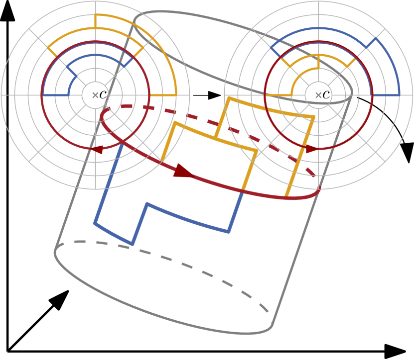
(a) Flipping the cylinder.

(b) The ortho-radial drawing before and after flipping.

Figure 3: Illustration of flipping the cylinder.

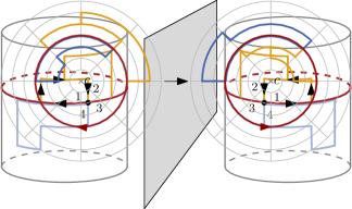
Figure 4: Mirroring the cylinder.

Lemma 3.1 (Flipping).

Let $\Gamma$ be an ortho-radial representation with outer face $f_{o}$ and central face $f_{c}$. If the cycle bounding the central face is not monotone, there exists an ortho-radial representation $\mkern 1.5mu\overline{\mkern-1.5mu\Gamma\mkern-1.5mu}\mkern 1.5mu$ such that

1. $\mkern 1.5mu\overline{\mkern-1.5muf\mkern-1.5mu}\mkern 1.5mu_{c}$ is the outer face of $\mkern 1.5mu\overline{\mkern-1.5mu\Gamma\mkern-1.5mu}\mkern 1.5mu$ and $\mkern 1.5mu\overline{\mkern-1.5muf\mkern-1.5mu}\mkern 1.5mu_{o}$ is the central face of $\mkern 1.5mu\overline{\mkern-1.5mu\Gamma\mkern-1.5mu}\mkern 1.5mu$,

2. $\mkern 1.5mu\overline{\mkern-1.5mu\ell\mkern-1.5mu}\mkern 1.5mu_{\mkern 1.5mu\overline{\mkern-1.5muC\mkern-1.5mu}\mkern 1.5mu}(\mkern 1.5mu\overline{\mkern-1.5mue\mkern-1.5mu}\mkern 1.5mu)=\ell_{C}(e)$ for all essential cycles $C$ and edges $e$ on $C$, where $\mkern 1.5mu\overline{\mkern-1.5mu\ell\mkern-1.5mu}\mkern 1.5mu$ is the labeling in $\mkern 1.5mu\overline{\mkern-1.5mu\Gamma\mkern-1.5mu}\mkern 1.5mu$.

In particular, increasing and decreasing cycles of $\Gamma$ correspond to increasing and decreasing cycles of $\mkern 1.5mu\overline{\mkern-1.5mu\Gamma\mkern-1.5mu}\mkern 1.5mu$, respectively.

Proof 3.2.

We define $\mkern 1.5mu\overline{\mkern-1.5mu\Gamma\mkern-1.5mu}\mkern 1.5mu$ as follows. The central face of $\Gamma$ becomes the outer face of $\mkern 1.5mu\overline{\mkern-1.5mu\Gamma\mkern-1.5mu}\mkern 1.5mu$ and the outer face of $\Gamma$ becomes the central face of $\mkern 1.5mu\overline{\mkern-1.5mu\Gamma\mkern-1.5mu}\mkern 1.5mu$. Further, we choose an arbitrary edge $e^{\star\star}$ on the central face $f_{c}$ of $\Gamma$ with $\ell_{f_{c}}(e^{\star\star})=0$ (such an edge exists since the cycle bounding the central face is not monotone), and choose $\mkern 1.5mu\overline{\mkern-1.5mue^{\star\star}\mkern-1.5mu}\mkern 1.5mu$ as the reference edge of $\mkern 1.5mu\overline{\mkern-1.5mu\Gamma\mkern-1.5mu}\mkern 1.5mu$. All other information of $\Gamma$ is transferred to $\mkern 1.5mu\overline{\mkern-1.5mu\Gamma\mkern-1.5mu}\mkern 1.5mu$ without modification. As the local structure is unchanged, $\mkern 1.5mu\overline{\mkern-1.5mu\Gamma\mkern-1.5mu}\mkern 1.5mu$ is an ortho-radial representation.

The essential cycles in $\Gamma$ bijectively correspond to the essential cycles in $\mkern 1.5mu\overline{\mkern-1.5mu\Gamma\mkern-1.5mu}\mkern 1.5mu$ by reversing the direction of the cycles. That is, any essential cycle $C$ in $\Gamma$ corresponds to the cycle $\mkern 1.5mu\overline{\mkern-1.5muC\mkern-1.5mu}\mkern 1.5mu$ in $\mkern 1.5mu\overline{\mkern-1.5mu\Gamma\mkern-1.5mu}\mkern 1.5mu$. Note that the reversal is necessary since we always consider essential cycles to be directed such that the center lies in its interior, which is defined as the area locally to the right of the cycle.

Consider any essential cycle $C$ in $\Gamma$. We denote the labeling of $C$ in $\Gamma$ by $\ell_{C}$ and the labeling of $\mkern 1.5mu\overline{\mkern-1.5muC\mkern-1.5mu}\mkern 1.5mu$ in $\mkern 1.5mu\overline{\mkern-1.5mu\Gamma\mkern-1.5mu}\mkern 1.5mu$ by $\mkern 1.5mu\overline{\mkern-1.5mu\ell\mkern-1.5mu}\mkern 1.5mu_{\mkern 1.5mu\overline{\mkern-1.5muC\mkern-1.5mu}\mkern 1.5mu}$. We show that for any edge $e$ on $C$ it is $\ell_{C}(e)=\mkern 1.5mu\overline{\mkern-1.5mu\ell\mkern-1.5mu}\mkern 1.5mu_{\mkern 1.5mu\overline{\mkern-1.5muC\mkern-1.5mu}\mkern 1.5mu}(\mkern 1.5mu\overline{\mkern-1.5mue\mkern-1.5mu}\mkern 1.5mu)$, which particularly implies that any monotone cycle in $\Gamma$ corresponds to a monotone cycle in $\mkern 1.5mu\overline{\mkern-1.5mu\Gamma\mkern-1.5mu}\mkern 1.5mu$ and vice versa. First, we pick a simple path $P$ from $e^{\star}$ to $e$ such that $P$ lies in the exterior of $C$ in $\Gamma$ and another simple path $Q$ from $e$ to $e^{\star\star}$ that lies in the interior of $C$.

Assume for now that $P+e+Q$ is simple. We shall see at the end how the proof can be extended if this is not the case. By the choice of $e^{\star\star}$, we have

$$0 =\ell_{f_{c}}(e^{\star\star})=\operatorname{rot}(e^{\star}+P+e+Q+e^{\star\star})=\operatorname{rot}(e^{\star}+P+e)+\operatorname{rot}(e+Q+e^{\star\star})$$ (1)

Hence, $\operatorname{rot}(e^{\star}+P+e)=\operatorname{rot}(\mkern 1.5mu\overline{\mkern-1.5mue^{\star\star}\mkern-1.5mu}\mkern 1.5mu+\mkern 1.5mu\overline{\mkern-1.5muQ\mkern-1.5mu}\mkern 1.5mu+\mkern 1.5mu\overline{\mkern-1.5mue\mkern-1.5mu}\mkern 1.5mu)$ and in total

$$\mkern 1.5mu\overline{\mkern-1.5mu\ell\mkern-1.5mu}\mkern 1.5mu_{\mkern 1.5mu\overline{\mkern-1.5muC\mkern-1.5mu}\mkern 1.5mu}(\mkern 1.5mu\overline{\mkern-1.5mue\mkern-1.5mu}\mkern 1.5mu)=\operatorname{rot}(\mkern 1.5mu\overline{\mkern-1.5mue^{\star\star}\mkern-1.5mu}\mkern 1.5mu+\mkern 1.5mu\overline{\mkern-1.5muQ\mkern-1.5mu}\mkern 1.5mu+\mkern 1.5mu\overline{\mkern-1.5mue\mkern-1.5mu}\mkern 1.5mu)=\operatorname{rot}(e^{\star}+P+e)=\ell_{C}(e).$$ (2)

Thus, any monotone cycle in $\Gamma$ corresponds to a monotone cycle in $\mkern 1.5mu\overline{\mkern-1.5mu\Gamma\mkern-1.5mu}\mkern 1.5mu$ and vice versa.

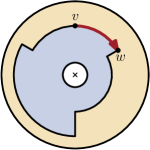
(a) The original graph with the essential cycle $C$.

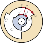
(b) The graph after it was cut at $C$.

Figure 5: Cutting the graph at an essential cycle $C$.

If $P+e+Q$ is not simple, we make it simple by cutting $G$ at $C$ such that the interior and the exterior of $C$ get their own copies of $C$; see Figure 5. We connect the two parts by an edge between two new vertices $x$ and $x^{\prime}$ on the two copies of $e$, which we denote by $vw$ in the exterior part and $v^{\prime}w^{\prime}$ in the interior part. The new edge is placed perpendicular to these copies. The path $P+vxx^{\prime}w^{\prime}+Q$ is simple and its rotation is $0$. Hence, the argument above implies $\mkern 1.5mu\overline{\mkern-1.5mu\ell\mkern-1.5mu}\mkern 1.5mu_{\mkern 1.5mu\overline{\mkern-1.5muC\mkern-1.5mu}\mkern 1.5mu}(\mkern 1.5mu\overline{\mkern-1.5mue\mkern-1.5mu}\mkern 1.5mu)=\ell_{C}(e)$.

Lemma 3.3 (Mirroring).

Let $\Gamma$ be an ortho-radial representation with outer face $f_{o}$ and central face $f_{c}$. There exists an ortho-radial representation $\hat{\Gamma}$ such that

1. $\mkern 1.5mu\overline{\mkern-1.5muf\mkern-1.5mu}\mkern 1.5mu_{o}$ is the outer face of $\hat{\Gamma}$ and $\mkern 1.5mu\overline{\mkern-1.5muf\mkern-1.5mu}\mkern 1.5mu_{c}$ is the central face of $\hat{\Gamma}$,

2. $\hat{\ell}_{\mkern 1.5mu\overline{\mkern-1.5muC\mkern-1.5mu}\mkern 1.5mu}(\mkern 1.5mu\overline{\mkern-1.5mue\mkern-1.5mu}\mkern 1.5mu)=-\ell_{C}(e)$ for all essential cycles $C$ and edges $e$ on $C$, where $\hat{\ell}$ is the labeling in $\hat{\Gamma}$.

In particular, increasing and decreasing cycles of $\Gamma$ correspond to decreasing and increasing cycles of $\hat{\Gamma}$, respectively.

Proof 3.4.

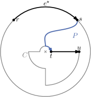
(a) The original graph with a path $P$ from the reference edge $e^{\star}$ to the edge $e$ on the essential cycle $C$.

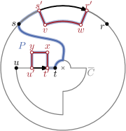
(b) The mirrored graph including the construction to extend the path $P$ to a path from $r^{\prime}$ to $u^{\prime}$.

Figure 6: The construction that is used to adapt the path from the reference edge to an edge $e$ on an essential cycle when the graph is mirrored.

We define $\hat{\Gamma}$ as follows. We reverse the direction of all faces and reverse the order of the edges around each vertex. The outer and central face are equal to those in $\Gamma$ (except for the directions) and the reference edge is $\mkern 1.5mu\overline{\mkern-1.5mue^{\star}\mkern-1.5mu}\mkern 1.5mu$. Since the reference edge is reversed, edges that point left in $\Gamma$ point right in $\hat{\Gamma}$ and vice versa, but the edges that point up (down) in $\Gamma$ also point up (down) in $\hat{\Gamma}$. Note that this construction satisfies the conditions for ortho-radial representations.

Let $e=tu$ be an edge on $C$ and $P$ a simple path from $e^{\star}=rs$ to $e=tu$ that lies in the exterior of $C$; we consider $P$ without $e^{\star}$ and $e$. In the mirrored representation $\hat{\Gamma}$ the direction of the reference edge and $C$ are reversed, i.e., the reference edge is $\mkern 1.5mu\overline{\mkern-1.5mue^{\star}\mkern-1.5mu}\mkern 1.5mu$, and we consider $\mkern 1.5mu\overline{\mkern-1.5muC\mkern-1.5mu}\mkern 1.5mu$. As $P$ starts at the tail of $\mkern 1.5mu\overline{\mkern-1.5mue^{\star}\mkern-1.5mu}\mkern 1.5mu$ and ends at the head of $\mkern 1.5mu\overline{\mkern-1.5mue\mkern-1.5mu}\mkern 1.5mu$, we cannot simply use $P$ to compute the label $\hat{\ell}_{\mkern 1.5mu\overline{\mkern-1.5muC\mkern-1.5mu}\mkern 1.5mu}(\mkern 1.5mu\overline{\mkern-1.5mue\mkern-1.5mu}\mkern 1.5mu)$.

Therefore, we modify $G$ and $\Gamma$ slightly by adding some vertices and edges as follows; see Figure 6. The edge $e^{\star}$ is subdivided by two new vertices $r^{\prime}$ and $s^{\prime}$, which are connected by a new path $s^{\prime}vwr^{\prime}$ in the interior of the graph. We place this path such that the face formed by this path and $r^{\prime}s^{\prime}$ is a rectangle. Similarly, we add the vertices $t^{\prime}$ and $u^{\prime}$ on $e$ and we connect $t^{\prime}$ to $u^{\prime}$ by a new path $t^{\prime}xyu^{\prime}$ such that the new face with these four vertices is a rectangle that lies in the exterior of $C$. We set $r^{\prime}s^{\prime}$ as the new reference edge and call the resulting representation $\Gamma^{\prime}$. Since $r^{\prime}s^{\prime}$ is a part of the original reference edge $e^{\star}$, this preserves the labelings. In particular, the labels of $tt^{\prime}$, $t^{\prime}u^{\prime}$ and $u^{\prime}u$ in $\Gamma^{\prime}$ are equal to $\ell_{C}(e)$ in $\Gamma$.

Setting $P^{\prime}=r^{\prime}wvs^{\prime}s+P+tt^{\prime}xyu^{\prime}$, we obtain a simple path in the mirrored representation of $\Gamma^{\prime}$ from the reference edge $\mkern 1.5mu\overline{\mkern-1.5mue^{\star}\mkern-1.5mu}\mkern 1.5mu$ to $\mkern 1.5mu\overline{\mkern-1.5mue\mkern-1.5mu}\mkern 1.5mu$. Since mirroring flips the sign of the rotation of a path, we get

$$\hat{\ell}_{\mkern 1.5mu\overline{\mkern-1.5muC\mkern-1.5mu}\mkern 1.5mu}(\mkern 1.5mu\overline{\mkern-1.5mue\mkern-1.5mu}\mkern 1.5mu) =\operatorname{rot}_{\hat{\Gamma^{\prime}}}(s^{\prime}r^{\prime}+P^{\prime}+u^{\prime}t^{\prime})=\operatorname{rot}_{\hat{\Gamma^{\prime}}}(s^{\prime}r^{\prime}vws^{\prime}s)+\operatorname{rot}_{\hat{\Gamma^{\prime}}}(s^{\prime}s+P+tt^{\prime})+\operatorname{rot}_{\hat{\Gamma^{\prime}}}(tt^{\prime}xyu^{\prime}t^{\prime})$$

$$=2-\operatorname{rot}_{\Gamma^{\prime}}(s^{\prime}s+P+tt^{\prime})-2=-\operatorname{rot}_{\Gamma}(e^{\star}+P+e)=-\ell_{C}(e).$$

In particular, increasing and decreasing cycles of $\Gamma$ correspond to decreasing and increasing cycles of $\hat{\Gamma}$, respectively.

We can further restrict ourselves to instances with minimum degree 2 by removing all degree-1 vertices in the following fashion. Suppose $v$ is a degree-1 vertex in $G$. It is not hard to see that $G$ contains a monotone cycle if and only if $G-v$ does. It is thus tempting to iteratively remove degree-1 vertices. However later, when we augment the graph and its ortho-radial representation so that all faces become rectangular, reinserting these vertices may require non-trivial modifications. To avoid this we present a transformation that produces a supergraph of a subdivision of $G$ where every vertex has degree 2.

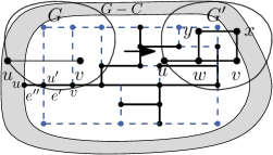
Figure 7: The degree-1 vertex $v$ is replaced by a rectangle.

Let $uv$ be the edge incident to the degree-1 vertex $v$. We obtain a graph $G^{\prime}$ from $G$ by subdividing $uv$ with a new vertex $w$, and adding two new vertices $x$ and $y$ along with edges $vx$, $xy$ and $wy$. Further, we obtain $\Gamma^{\prime}$ from $\Gamma$ by setting all angles in the inner face bounded by $v,w,x,y$ to $90\degree$; see Fig. 7. It is easy to see that $\Gamma^{\prime}$ is valid if and only if $\Gamma$ is, since a monotone cycle of $G$ is also a monotone cycle of $G^{\prime}$, and conversely, since $uw$ is a bridge, a cycle $C$ of $G^{\prime}$ is either $w,v,x,y$ or it is contained in $G-uv$. The former cycle is non-essential by construction, and hence any monotone cycle of $G^{\prime}$ is also a monotone cycle of $G$. It follows that the monotone cycles of $G$ bijectively correspond to the monotone cycles of $G^{\prime}$. Iteratively applying this construction to all degree-1 vertices yields the following lemma.

Lemma 3.5.

Let $G$ be a planar 4-graph on $n$ vertices with ortho-radial representation $\Gamma$. In $O(n)$ time we can compute a supergraph $G^{*}$ with minimum degree 2 of a subdivision of $G$ with ortho-radial representation $\Gamma^{*}$ such that there is a bijective correspondence between monotone cycles in $G$ and monotone cycles in $G^{*}$.

4 Finding Monotone Cycles

The two conditions for ortho-radial representations are local and checking them can easily be done in linear time. We therefore assume in this section that we are given a planar 4-graph $G$ with an ortho-radial representation $\Gamma$. The condition for validity however references all essential cycles of which there may be exponentially many. We present an algorithm that checks whether $\Gamma$ contains a monotone cycle and computes such a cycle if one exists. The main difficulty is that the labels on a decreasing cycle $C$ depend on an elementary path $P$ from the reference edge to $C$. However, we know neither the path $P$ nor the cycle $C$ in advance, and choosing a specific cycle $C$ may rule out certain paths $P$ and vice versa.

We only describe how to search for decreasing cycles; increasing cycles can be found by searching for decreasing cycles in the mirrored representation by Lemma 3.3. A decreasing cycle $C$ is outermost if it is not contained in the interior of any other decreasing cycle. Clearly, if $\Gamma$ contains a decreasing cycle, then it also has an outermost one. We first show that in this case this cycle is uniquely determined.

Lemma 4.1.

If $\Gamma$ contains a decreasing cycle, there is a unique outermost decreasing cycle.

Proof 4.2.

Assume that $\Gamma$ has two outermost decreasing cycles $C_{1}$ and $C_{2}$, i.e., $C_{1}$ does not lie in the interior of $C_{2}$ and vice versa. Let $C$ be the cycle bounding the outer face of the subgraph $H=C_{1}+C_{2}$ that is formed by the two decreasing cycles. By construction, $C_{1}$ and $C_{2}$ lie in the interior of $C$, and we claim that $C$ is a decreasing cycle contradicting that $C_{1}$ and $C_{2}$ are outermost. To that end, we show that $\ell_{C}(e)=\ell_{C_{1}}(e)$ for any edge $e$ that belongs to both $C$ and $C_{1}$, and $\ell_{C}(e)=\ell_{C_{2}}(e)$ for any edge $e$ that belongs to both $C$ and $C_{2}$. Hence, all edges of $C$ have a non-negative label since $C_{1}$ and $C_{2}$ are decreasing. By Proposition 2.3 there is at least one label of $C$ that is positive, and hence $C$ is a decreasing cycle.

It remains to show that $\ell_{C}(e)=\ell_{C_{1}}(e)$ for any edge $e$ that belongs to both $C$ and $C_{1}$; the case that $e$ belongs to both $C$ and $C_{2}$ can be handled analogously. Let $\Gamma_{H}$ be the ortho-radial representation $\Gamma$ restricted to $H$. We flip the cylinder to exchange the outer face with the central face and vice versa. More precisely, Lemma 3.1 implies that the reverse edge $\mkern 1.5mu\overline{\mkern-1.5mue\mkern-1.5mu}\mkern 1.5mu$ of $e$ lies on the central face of the flipped representation $\mkern 1.5mu\overline{\mkern-1.5mu\Gamma\mkern-1.5mu}\mkern 1.5mu_{H}$ of $\Gamma_{H}$. Further, it proves that $\mkern 1.5mu\overline{\mkern-1.5mu\ell\mkern-1.5mu}\mkern 1.5mu_{\mkern 1.5mu\overline{\mkern-1.5muC\mkern-1.5mu}\mkern 1.5mu}(\mkern 1.5mu\overline{\mkern-1.5mue\mkern-1.5mu}\mkern 1.5mu)=\ell_{C}(e)$ and $\mkern 1.5mu\overline{\mkern-1.5mu\ell\mkern-1.5mu}\mkern 1.5mu_{\mkern 1.5mu\overline{\mkern-1.5muC_{1}\mkern-1.5mu}\mkern 1.5mu}(\mkern 1.5mu\overline{\mkern-1.5mue\mkern-1.5mu}\mkern 1.5mu)=\ell_{C_{1}}(e)$, where $\mkern 1.5mu\overline{\mkern-1.5mu\ell\mkern-1.5mu}\mkern 1.5mu$ is the labeling in $\mkern 1.5mu\overline{\mkern-1.5mu\Gamma\mkern-1.5mu}\mkern 1.5mu_{H}$. Hence, by Proposition 2.2 we obtain $\mkern 1.5mu\overline{\mkern-1.5mu\ell\mkern-1.5mu}\mkern 1.5mu_{\mkern 1.5mu\overline{\mkern-1.5muC\mkern-1.5mu}\mkern 1.5mu}(\mkern 1.5mu\overline{\mkern-1.5mue\mkern-1.5mu}\mkern 1.5mu)=\mkern 1.5mu\overline{\mkern-1.5mu\ell\mkern-1.5mu}\mkern 1.5mu_{\mkern 1.5mu\overline{\mkern-1.5muC_{1}\mkern-1.5mu}\mkern 1.5mu}(\mkern 1.5mu\overline{\mkern-1.5mue\mkern-1.5mu}\mkern 1.5mu)$. Flipping back the cylinder, again by Lemma 3.1 we obtain $\ell_{C}(e)=\ell_{C_{1}}(e)$.

The core of our algorithm is an adapted left-first DFS. Given a directed edge $e$ it determines the outermost decreasing cycle $C$ in $\Gamma$ such that $C$ contains $e$ in the given direction and $e$ has the smallest label among all edges on $C$, if such a cycle exists. By running this test for each directed edge of $G$ as the start edge, we find a decreasing cycle if one exists.

Our algorithm is based on a DFS that visits each vertex at most once. A left-first search maintains for each visited vertex $v$ a reference edge $\lx@mung@bibliography@pre\thebibliography\lx@bibitem{(}v)$, the edge of the search tree via which $v$ was visited. Whenever it has a choice which vertex to visit next, it picks the first outgoing edge in clockwise direction after the reference edge that leads to an unvisited vertex. In addition to that, we employ a filter that ignores certain outgoing edges during the search. To that end, we define for all outgoing edges $e$ incident to a visited vertex $v$ a search label $\tilde{\ell}(e)$ by setting $\tilde{\ell}(e)=\tilde{\ell}(\lx@mung@bibliography@pre\thebibliography\lx@bibitem{(}v))+\operatorname{rot}(\lx@bibitem{(}v)+e)$ for each outgoing edge $e$ of $v$. In our search we ignore edges with negative search labels. For a given directed edge $vw$ in $G$ we initialize the search by setting $\lx@mung@bibliography@pre\thebibliography\lx@bibitem{(}w)=vw$, $\tilde{\ell}(vw)=0$ and then start searching from $w$.

Let $T$ denote the directed search tree with root $w$ constructed by the DFS in this fashion. If $T$ contains $v$, then this determines a candidate cycle $C$ containing the edge $vw$. If $C$ is a decreasing cycle, which we can easily check by determining an elementary path from the reference edge to $C$, we report it. Otherwise, we show that there is no outermost decreasing cycle $C$ such that $vw$ lies on $C$ and has the smallest label among all edges on $C$.

It is necessary to check that $C$ is essential and decreasing. For example the cycle in Figure 9 is found by the search and though it is essential, it is non-decreasing. This is caused by the fact that the label of $vw$ is actually $-4$ on this cycle but the search assumes it to be $0$.

Figure 8: The search from $vw$ finds the non-decreasing cycle $C$. Edges are labeled $\ell_{C}(e)/\tilde{\ell}(e)$.

Figure 9: Path $Q$ and its prefix $P$ that leaves $C$ once and ends at a vertex $p$ of $C$.

Lemma 4.3.

Assume $\Gamma$ contains a decreasing cycle. Let $C$ be the outermost decreasing cycle of $\Gamma$ and let $vw$ be an edge on $C$ with the minimum label, i.e., $\ell_{C}(vw)\leq\ell_{C}(e)$ for all edges $e$ of $C$. Then the left-first DFS from $vw$ finds $C$.

Proof 4.4.

Assume that the search does not find $C$. Let $T$ be the tree formed by the edges visited by the search. Since the search does not find $C$ by assumption, a part of $C[w,v]$ does not belong to $T$. Let $xy$ be the first edge on $C[w,v]$ that is not visited, i.e., $C[w,x]$ is a part of $T$ but $xy\not\in T$. There are two possible reasons for this. Either $\tilde{\ell}(xy)<0$ or $y$ has already been visited before via another path $Q$ from $w$ with $Q\neq C[w,y]$. The case $\tilde{\ell}(xy)<0$ can be excluded as follows. By the construction of the labels $\tilde{\ell}$, for any path $P$ from $w$ to a vertex $z$ in $T$ and any edge $e^{\prime}$ incident to $z$ we have $\tilde{\ell}(e^{\prime})=\operatorname{rot}(vw+P+e^{\prime})$. In particular, $\tilde{\ell}(xy)=\operatorname{rot}(C[vw,xy])=\ell_{C}(xy)-\ell_{C}(vw)\geq 0$ since the rotation can be rewritten as a label difference (see [3, Obs. 7]) and $vw$ has the smallest label on $C$.

Hence, $T$ contains a path $Q$ from $w$ to $x$ that was found by the search before and $Q$ does not completely lie on $C$. There is a prefix of $Q$ (possibly of length $0$) lying on $C$ followed by a subpath not on $C$ until the first vertex $p$ of $Q$ that again belongs to $C$; see Figure 9. We set $P=Q[w,p]$ and denote the vertex where $P$ leaves $C$ by $b$. By construction the edge $vw$ lies on $C[p,b]$. The subgraph $H=P+C$ that is formed by the decreasing cycle $C$ and the path $P$ consists of the three internally vertex-disjoint paths $P[b,p]$, $C[b,p]$ and $\mkern 1.5mu\overline{\mkern-1.5muC\mkern-1.5mu}\mkern 1.5mu[b,p]$ between $b$ and $p$. Since edges that are further left are preferred during the search, the clockwise order of these paths around $b$ and $p$ is fixed. In $H$ there are three faces, bounded by $C$, $\mkern 1.5mu\overline{\mkern-1.5muC\mkern-1.5mu}\mkern 1.5mu[b,p]+\mkern 1.5mu\overline{\mkern-1.5muP\mkern-1.5mu}\mkern 1.5mu[p,b]$ and $P[b,p]+\mkern 1.5mu\overline{\mkern-1.5muC\mkern-1.5mu}\mkern 1.5mu[p,b]$, respectively. Since $C$ is an essential cycle and a face in $H$, it is the central face and one of the two other faces is the outer face. These two possibilities are shown in Figure 10. We denote the cycle bounding the outer face but in which the edges are directed such that the outer face lies locally to the left by $C^{\prime}$. That is, the boundary of the outer face is $\mkern 1.5mu\overline{\mkern-1.5muC^{\prime}\mkern-1.5mu}\mkern 1.5mu$. We distinguish cases based on which of the two possible cycles constitutes $\mkern 1.5mu\overline{\mkern-1.5muC^{\prime}\mkern-1.5mu}\mkern 1.5mu$.

(a) The edge $vw$ lies on the outer face of $H$.

(b) The edge $vw$ does not lie on the outer face of $H$.

Figure 10: The two possible embeddings of the subgraph formed by the decreasing cycle $C$ and the path $P$, which was found by the search.

If $\mkern 1.5mu\overline{\mkern-1.5muC^{\prime}\mkern-1.5mu}\mkern 1.5mu=\mkern 1.5mu\overline{\mkern-1.5muC\mkern-1.5mu}\mkern 1.5mu[b,p]+\mkern 1.5mu\overline{\mkern-1.5muP\mkern-1.5mu}\mkern 1.5mu[p,b]$ forms the outer face of $H$, $vw$ lies on $C^{\prime}$ as illustrated in Figure 10(a) and we show that $C^{\prime}$ is a decreasing cycle, which contradicts the assumption that $C$ is the outermost decreasing cycle. Since $P$ is simple and lies in the exterior of $C$, the path $P$ is contained in $C^{\prime}$, which means $C^{\prime}[w,p]=P$. The other part of $C^{\prime}$ is formed by $C[p,w]$. Since $C$ forms the central face of $H$, the labels of the edges on $C[p,w]$ are the same for $C$ and $C^{\prime}$ by Proposition 2.2. In particular, $\ell_{C}(vw)=\ell_{C^{\prime}}(vw)$ and all the labels of edges on $C[p,w]$ are non-negative because $C$ is decreasing. The label of any edge $e$ on both $C^{\prime}$ and $P$ is $\ell_{C^{\prime}}(e)=\ell_{C^{\prime}}(vw)+\operatorname{rot}(vw+P[w,e])=\ell_{C}(vw)+\tilde{\ell}(e)\geq 0$. Thus, the labeling of $C^{\prime}$ is non-negative. Further, not all labels of $C^{\prime}$ are $0$ since otherwise $C$ would not be a decreasing cycle by Proposition 2.3. Hence, $C^{\prime}$ is decreasing and contains $C$ in its interior, a contradiction.

If $\mkern 1.5mu\overline{\mkern-1.5muC^{\prime}\mkern-1.5mu}\mkern 1.5mu=\mkern 1.5mu\overline{\mkern-1.5muC\mkern-1.5mu}\mkern 1.5mu[p,b]+P[b,p]$, the edge $vw$ does not lie on $C^{\prime}$; see Figure 10(b). We show that $C^{\prime}$ is a decreasing cycle containing $C$ in its interior, again contradicting the choice of $C$. As above, Proposition 2.2 implies that the common edges of $C$ and $C^{\prime}$ have the same labels on both cycles. It remains to show that all edges $xy$ on $\mkern 1.5mu\overline{\mkern-1.5muP\mkern-1.5mu}\mkern 1.5mu[p,b]$ have non-negative labels. To establish this we use paths to the edge that follows $b$ on $C$. This edge $bc$ has the same label on both cycles and thus provides a handle on $\ell_{C^{\prime}}(xy)$. We make use of the following equations, which follow immediately from the definition of the (search) labels.

$$\ell_{C^{\prime}}(bc) =\ell_{C^{\prime}}(xy)+\operatorname{rot}(\mkern 1.5mu\overline{\mkern-1.5muP\mkern-1.5mu}\mkern 1.5mu[xy,db])+\operatorname{rot}(dbc)=\ell_{C^{\prime}}(xy)-\operatorname{rot}(P[bd,yx])-\operatorname{rot}(cbd)$$

$$\ell_{C}(bc) =\ell_{C}(vw)+\operatorname{rot}(C[vw,ab])+\operatorname{rot}(abc)$$

$$\tilde{\ell}(yx) =\operatorname{rot}(C[vw,ab])+\operatorname{rot}(abd)+\operatorname{rot}(P[bd,yx])$$

Since $\ell_{C}(bc)=\ell_{C^{\prime}}(bc)$ and $\operatorname{rot}(abd)=-\operatorname{rot}(dba)$, we thus get

$$\ell_{C^{\prime}}(xy) =\ell_{C}(vw)+\operatorname{rot}(C[vw,ab])+\operatorname{rot}(abc)+\operatorname{rot}(P[bd,yx])+\operatorname{rot}(cbd)$$

$$=\ell_{C}(vw)+\tilde{\ell}(yx)+\operatorname{rot}(dba)+\operatorname{rot}(abc)+\operatorname{rot}(cbd).$$

Since $\ell_{C}(vw)\geq 0$ and $\tilde{\ell}(yx)\geq 0$ (as $yx$ was not filtered out), it follows that $\ell_{C^{\prime}}(xy)\geq\operatorname{rot}(abc)+\operatorname{rot}(dba)+\operatorname{rot}(cbd)=2$ as this is the sum of clockwise rotations around a degree-3 vertex. Hence, $C^{\prime}$ is decreasing and contains $C$ in its interior, a contradiction. Since both embeddings of $H$ lead to a contradiction, we obtain a contradiction to our initial assumption that the search fails to find $C$.

The left-first DFS clearly runs in $O(n)$ time. In order to guarantee that the search finds a decreasing cycle if one exists, we run it for each of the $O(n)$ directed edges of $G$. Since some edge must have the lowest label on the outermost decreasing cycle, Lemma 4.3 guarantees that we eventually find a decreasing cycle if one exists. Increasing cycles can be found by finding decreasing cycles in the mirror representation $\hat{\Gamma}$ (Lemma 3.3).

Theorem 4.5.

Let $G$ be a planar 4-graph on $n$ vertices and let $\Gamma$ be an ortho-radial representation of $G$. It can be determined in $O(n^{2})$ time whether $\Gamma$ is valid.

5 Rectangulation

(a) Multiple edge candidates.

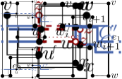
(b) Vertical.

(c) Horizontal.

(d) Horizontal.

(e) Horizontal.

Figure 11: Examples of augmentations. (11(a)) The candidate edges of $u$ are $e_{1}$, $e_{2}$ and $e_{3}$. (11(b)) Insertion of vertical edge $uz$. (11(c)) $\Gamma^{u}_{vw}$ contains a decreasing cycle. (11(d)) $\Gamma^{u}_{vw}$ is valid. (11(e)) Insertion of horizontal edge $uw_{i}$ because there is a horizontal path from $w_{i}$ to $u$.

The core of the algorithm for drawing a valid ortho-radial representation $\Gamma$ of a graph $G$ by Barth et al. [2] is a rectangulation procedure that successively augments $G$ with new vertices and edges to a graph $G^{*}$ along with a valid ortho-radial representation $\Gamma^{*}$ where every face of $G^{*}$ is a rectangle. A regular face is a rectangle if it has exactly four turns, which are all right turns. The outer and central faces are rectangles if they have no turns. The ortho-radial representation $\Gamma^{*}$ is then drawn by computing flows in two flow networks [3, Thm. 18].

To facilitate the analysis, we briefly sketch the augmentation procedure. Here it is crucial that we assume our instances to be normalized; in particular they do not have degree-1 vertices. The augmentation algorithm works by augmenting non-rectangular faces one by one, thereby successively removing concave angles at the vertices until all faces are rectangles. Consider a face $f$ with a left turn (i.e., a concave angle) at $u$ such that the following two turns when walking along $f$ (in clockwise direction) are right turns; see Figure 11. We call $u$ a port of $f$. We define a set of candidate edges that contains precisely those edges $vw$ of $f$, for which $\operatorname{rot}(f[u,vw])=2$; see Figure 11(a). We treat this set as a sequence, where the edges appear in the same order as in $f$, beginning with the first candidate after $u$. The augmentation $\Gamma^{u}_{vw}$ with respect to a candidate edge $vw$ is obtained by splitting the edge $vw$ into the edges $vz$ and $zw$, where $z$ is a new vertex, and adding the edge $uz$ in the interior of $f$ such that the angle formed by $zu$ and the edge following $u$ on $f$ is $90\degree$. The direction of the new edge $uz$ in $\Gamma^{u}_{vw}$ is the same for all candidate edges. If this direction is vertical, we call $u$ a vertical port and otherwise a horizontal port. We note that any vertex with a concave angle in a face becomes a port during the augmentation process. In particular, the incoming edge of the vertex determines whether the port is horizontal or vertical. The condition for candidates guarantees that $\Gamma^{u}_{vw}$ is an ortho-radial representation. It may, however, not be valid. The crucial steps in [2] are establishing the following facts.

1. Let $u$ be a vertical port. Augmenting with the first candidate never produces a monotone cycle [3, Lemma 21].

2. Let $u$ be a horizontal port. Augmenting with the first candidate never produces an increasing cycle [3, Lemma 22] and augmenting with the last candidate never produces a decreasing cycle [3, Lemma 24].

3. Let $u$ be a horizontal port. If two consecutive candidates $e_{i}=v_{i}w_{i}$ and $e_{i+1}=v_{i+1}w_{i+1}$ produce a decreasing and an increasing cycle, respectively, then $w_{i}$, $v_{i+1}$ and $u$ lie on a path that starts at $w_{i}$ or $v_{i+1}$, and whose edges all point right; see Figure 11(e). A suitable augmentation can be found in $O(n)$ time. [3, Lemmas 25, 26].

It thus suffices to test for each candidate whether $\Gamma^{u}_{vw}$ is valid until either such a valid augmentation is found or we find two consecutive candidate edges where the first produces a decreasing cycle and the second produces an increasing cycle. Then, Fact 3 yields the desired valid augmentation. Since each valid augmentation reduces the number of concave angles, we obtain a rectangulation after $O(n)$ valid augmentations. Moreover, there are $O(n)$ candidates for each augmentation, each of which can be tested for validity (and increasing/decreasing cycles can be detected) in $O(n^{2})$ time by Theorem 4.5. Thus, the augmentation algorithm can be implemented to run in $O(n^{4})$ time.

In the remainder of this section we present an improvement to $O(n^{2})$ time, which is achieved in two steps. First, we show that due to the nature of augmentations the validity test can be done in $O(n)$ time (Section 5.1). Second, for each augmentation we execute a post-processing that reduces the number of validity tests to $O(n)$ in total (Section 5.2).

5.1 1st Improvement – Faster Validity Test

The general test for monotone cycles performs one left-first depth first search per edge and runs in $O(n^{2})$ time. However, we can exploit the special structure of the augmentation to reduce the running time to $O(n)$. For the proof we restrict ourselves to the case that the inserted edge $uz$ points to the right. The case that it points left can be handled by flipping the representation using Lemma 3.1.

The key result is that in any decreasing cycle of an augmentation the new edge $uz$ has the minimum label. Thus, performing only one left-first DFS starting at $uz$ is sufficient. For increasing cycles the arguments do not hold, but in a second step we show that the test for increasing cycles can be replaced by a simple test for horizontal paths.

Recall that the augmentations $\Gamma^{u}_{vw}$ that are tested during the rectangulation are built by adding one edge $uz$ to a valid representation $\Gamma$. Hence, any monotone cycle in $\Gamma^{u}_{vw}$ contains the edge $uz$.

We first show that the new edge $uz$ has label $0$ on any decreasing cycle in the augmentation $\Gamma^{u}_{vw}$ if $vw$ is the first candidate. We extend this result afterwards to augmentations to all candidates. Since the label of edges on decreasing cycles is non-negative, this implies in particular that the label of $uz$ is minimum, which is sufficient for the left-first DFS to succeed (see Lemma 4.3).

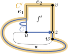
Figure 12: A decreasing cycle $C$ that uses $uz$ and an essential cycle $C^{\prime}$ derived from $C$.

Lemma 5.1.

Let $vw$ be the first candidate on $f$ after $u$. If $\Gamma^{u}_{vw}$ contains a decreasing cycle $C$, then $C$ contains $uz$ in this direction and $\ell_{C}(uz)=0$.

Proof 5.2.

This proof uses ideas from the proof of Lemma 22 of [3]. We first consider the case that $C$ uses $uz$ (and not $zu$) and assume for the sake of contradiction that $\ell_{C}(uz)\neq 0$; see Figure 12. Since $uz$ points right, $\ell_{C}(uz)$ is divisible by $4$. Together with $\ell_{C}(uz)\geq 0$ because $C$ is decreasing, we obtain $\ell_{C}(uz)\geq 4$. By Lemma 14 of [3] there is an essential cycle $C^{\prime}$ without $uz$ in the subgraph $H$ that is formed by the new rectangular face $f^{\prime}$ and $C$. The labels of any common edge $e$ of $C$ and $C^{\prime}$ are equal and $\ell_{C^{\prime}}(e)=\ell_{C}(e)\geq 0$. All other edges of $C^{\prime}$ lie on $f^{\prime}$. Since $f^{\prime}$ is rectangular, the labels of these edges differ by at most $1$ from $\ell_{C}(uz)$. By assumption it is $\ell_{C}(uz)\geq 4$ and therefore $\ell_{C^{\prime}}(e)\geq 3$ for all edges $e\in C^{\prime}\cap f^{\prime}$. Hence, $C^{\prime}$ is a decreasing cycle in $G$ contradicting the validity of $\Gamma$.

If $zu\in C$, it is $\ell_{C}(zu)\geq 2$ and a similar argument yields a decreasing cycle in $\Gamma$.

While the same statement does not generally hold for all candidates, it does hold if the first candidate creates a decreasing cycle.

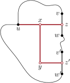
Figure 13: The structure used to simulate the simultaneous insertion of $uz$ to $vw$ and $uz^{\prime}$ to $v^{\prime}w^{\prime}$.

Lemma 5.3.

Let $vw$ be the first candidate and $v^{\prime}w^{\prime}$ be another candidate. Denote the edge inserted in $\Gamma^{u}_{v^{\prime}w^{\prime}}$ by $uz^{\prime}$. If $\Gamma^{u}_{vw}$ contains a decreasing cycle, any decreasing cycle $C^{\prime}$ in $\Gamma^{u}_{v^{\prime}w^{\prime}}$ uses $uz^{\prime}$ in this direction and $\ell_{C^{\prime}}(uz^{\prime})=0$.

Proof 5.4.

In order to simulate the insertion of two new edges to both $vw$ and $v^{\prime}w^{\prime}$ we use the structure from the proof of Lemma 25 of [3]; see Figure 13. We denote the resulting augmented representation by $\tilde{\Gamma}$. There is a one-to-one correspondence between decreasing cycles in $\Gamma^{u}_{vw}$ and decreasing cycles in $\tilde{\Gamma}$ containing $uxz$. Let $C$ be a decreasing cycle in $\tilde{\Gamma}$ containing $uxz$. By Lemma 5.1 the cycle $C$ contains $uxz$ in this direction, and we have $\ell_{C}(ux)=0$.

Similarly, for any decreasing cycle in $\Gamma^{u}_{v^{\prime}w^{\prime}}$ there is a decreasing cycle in $\tilde{\Gamma}$ where $uz^{\prime}$ ($z^{\prime}u$) is replaced by the path $uxyz^{\prime}$ ($z^{\prime}yxu$). Let $\tilde{C^{\prime}}$ be the decreasing cycle in $\tilde{\Gamma}$ that corresponds to the decreasing cycle $C^{\prime}$ in $\Gamma^{u}_{v^{\prime}w^{\prime}}$. We have $\ell_{\tilde{C^{\prime}}}(ux)=\ell_{C^{\prime}}(uz^{\prime})$.

Suppose for now that $C^{\prime}$ uses $uz^{\prime}$ in this direction, which means that $\tilde{C^{\prime}}$ uses $ux$. Let $\tilde{f}$ be the central face of $H=C+\tilde{C^{\prime}}$. Either $ux$ lies on the boundary of $\tilde{f}$ or not. Assume for the sake of contradiction that $ux$ does not lie on $\tilde{f}$. Then, $\tilde{f}$ includes neither $xz$, $xy$ nor $yz^{\prime}$. Hence, $\tilde{f}$ is formed exclusively by edges that are present in $G$. Since $\Gamma$ is valid, either all labels of $\tilde{f}$ are $0$ or there is an edge on $\tilde{f}$ with a negative label.

In the first case there is an edge $e$ of $C$ leaving $\tilde{f}$, i.e., $e$ starts at a vertex of $\tilde{f}$ and ends at a vertex in the exterior of $\tilde{f}$. If no such edge existed, $\tilde{f}$ would be formed exclusively by edges of $C$ or exclusively by edges of $\tilde{C^{\prime}}$. This would imply that one of these cycles is not simple. But for that edge $e$ it is $\ell_{C}(e)=-1$ contradicting the assumption that $C$ is decreasing.

In the second case there is an edge $e$ on $\tilde{f}$ with $\ell_{\tilde{f}}(e)<0$. This edge belongs to at least one of the cycles $C$ and $\tilde{C^{\prime}}$, say $C$. But then it is $\ell_{C}(e)=\ell_{\tilde{f}}(e)<0$ by Proposition 2.2, contradicting again that $C$ is decreasing. Thus, $ux$ lies on $\tilde{f}$, and therefore we obtain from Proposition 2.2 that $\ell_{\tilde{C^{\prime}}}(ux)=\ell_{C}(ux)=0$, where the last equality follows from Lemma 5.1.

Above we assumed that $\tilde{C^{\prime}}$ uses $ux$ in this direction. This is in fact the only possibility. Assume for the sake of contradiction that $xu\in\tilde{C^{\prime}}$. If $ux$ does not lie on the central face $\tilde{f}$ (in any direction), we obtain a contradiction as above. Since $C$ is essential and includes $ux$, the central face lies locally to the right of $ux$. Similarly, $\tilde{C^{\prime}}$ is essential and contains $xu$. Therefore, the central face lies to the right of $xu$ and thus to the left of $ux$. As $\tilde{f}$ cannot be both to the left and the right of $ux$, we have a contradiction.

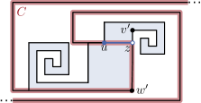
Figure 14: Here, the insertion of the edge $uz$ to the last candidate $v^{\prime}w^{\prime}$ introduces an increasing cycle $C$ with $\ell_{C}(uz)=-4$.

Altogether, we can efficiently test which of the candidates $e_{1},\dots,e_{k}$ produce decreasing cycles as follows. By Lemma 5.1, if the first candidate is not valid, then $\Gamma^{u}_{e_{1}}$ has a decreasing cycle that contains the new edge $uz$ with label $0$, which is hence the minimum label for all edges on the cycle. This can be tested in $O(n)$ time by Lemma 4.3. Fact 2 guarantees that we either find a valid augmentation or a decreasing cycle. In the former case we are done, in the second case Lemma 5.3 allows us to similarly restrict the labels of $uz$ to $0$ for the remaining candidate edges, thus allowing us to detect decreasing cycles in $\Gamma^{u}_{e_{i}}$ in $O(n)$ time for $i=2,\dots,k$.

It is tempting to use the mirror symmetry (Lemma 3.3, Appendix 3) to exchange increasing and decreasing cycles to deal with increasing cycles in an analogous fashion. However, this fails as mirroring invalidates the property that $u$ is followed by two right turns in clockwise direction. For example, in Figure 14 inserting the edge to the last candidate introduces an increasing cycle $C$ with $\ell_{C}(uz)=-4$. We therefore give a direct algorithm for detecting increasing cycles in this case.

Let $e_{i}=v_{i}w_{i}$ and $e_{i+1}={v_{i+1}w_{i+1}}$ be two consecutive candidates for $u$ such that $\Gamma^{u}_{e_{i}}$ contains a decreasing cycle but $\Gamma^{u}_{e_{i+1}}$ does not. If $\Gamma^{u}_{e_{i+1}}$ contains an increasing cycle, then by Fact 3 the vertices $w_{i}$, $v_{i+1}$ and $u$ lie on a path that starts at $w_{i}$ or $v_{i+1}$, and whose edges all point right. The presence of such a horizontal path $P$ can clearly be checked in linear time, thus allowing us to also detect increasing cycles provided that the previous candidate produced a decreasing cycle. If $P$ exists, we insert the edge $uw_{i}$ or $uv_{i+1}$ depending on whether $P$ starts at $w_{i}$ or $v_{i+1}$, respectively; see Figure 11(e) for the first case. By Proposition 2.3 this does not produce monotone cycles. Otherwise, if $P$ does not exist, the augmentation $\Gamma^{u}_{e_{i+1}}$ is valid. In both cases we have resolved the horizontal port $u$ successfully.

Summarizing, the overall algorithm for augmenting from a horizontal port $u$ now works as follows. By exploiting Lemmas 5.1 and 5.3, we test the candidates in the order as they appear on $f$ until we find the first candidate $e$ for which $\Gamma^{u}_{e}$ does not contain a decreasing cycle. Using Fact 3 we either find that $\Gamma^{u}_{e}$ is valid, or we find a horizontal path as described above. In both cases this allows us to determine an edge whose insertion does not introduce a monotone cycle. Since in each test for a decreasing cycle the edge $uz$ can be restricted to have label $0$, each of the tests takes linear time. This improves the running time of the rectangulation algorithm to $O(n^{3})$.

Instead of linearly searching for a suitable candidate for $u$ we can employ a binary search on the candidates, which reduces the number of validity tests for $u$ from linear to logarithmic. To do this efficiently we first compute the list of all candidates $e_{1},\dots,e_{k}$ for $u$ in time linear to the size of $f$. Next, we test if the augmentation $\Gamma^{u}_{e_{1}}$ is valid. If it is, we are done.

Otherwise, we start the binary search on the list $e_{1},\dots,e_{k}$, where $k$ is the number of candidates for $u$. The search maintains a sublist $e_{i},\dots,e_{j}$ of consecutive candidates such that $\Gamma^{u}_{e_{i}}$ contains a decreasing cycle and $\Gamma^{u}_{e_{j}}$ does not. Note that this invariant holds in the beginning because we explicitly test for a decreasing cycle in $\Gamma^{u}_{e_{1}}$ and there is no decreasing cycle in $\Gamma^{u}_{e_{k}}$ by Fact 2. If the list consists of only two consecutive candidates, i.e., $j=i+1$, we stop. Otherwise, we set $m=\lfloor(i+j)/2\rfloor$ and test if $\Gamma^{u}_{e_{m}}$ contains a decreasing cycle. If it does, we recurse on $e_{m},\dots,e_{j}$ and otherwise on $e_{i},\dots,e_{m}$. As the invariant is preserved we end up with two consecutive candidates $e_{i}$ and $e_{i+1}$ such that $\Gamma^{u}_{e_{i}}$ contains a decreasing cycle and $\Gamma^{u}_{e_{i+1}}$ does not. In this situation Fact 3 guarantees that we find a valid augmentation.

Note that this augmentation may be different from the one we obtain if we test all candidates sequentially since there might be a candidate with a valid augmentation between two candidates whose augmentations contain decreasing cycles.

Lemma 5.5.

Using binary search we find a valid augmentation for $u$ in $O(n\log n)$ time.

Proof 5.6.

If the augmentation to the first candidate does not contain a decreasing cycle, it is valid by Fact 2, and we are done. Otherwise, the invariant that the augmentation for the first candidate in the list contains a decreasing cycle and the augmentation for the last candidate does not guarantee that we end up in a situation where we find a valid augmentation by Fact 3. This establishes the correctness of the augmentation algorithm based on binary search.

Applying Lemma 5.1 testing the first candidate requires $O(n)$ time. If this augmentation contains a decreasing cycle, Lemma 5.3 guarantees that all other tests for decreasing cycles can be implemented in $O(n)$ time as well. The final test for an increasing cycle can be replaced by a test for a horizontal path by Fact 3. In total, there are $O(\log n)$ tests with a total running time of $O(n\log n)$.

Since there are at most $n$ ports to remove, we obtain that any $4$-planar graph with valid ortho-radial representation can be rectangulated in $O(n^{2}\log n)$ time. Using Corollary 19 from [3] this further implies that a corresponding ortho-radial drawing can be computed in $O(n^{2}\log n)$ time.

Theorem 5.7.

Given a valid ortho-radial representation $\Gamma$ of a graph $G$, a corresponding rectangulation can be computed in $O(n^{2}\log n)$ time.

5.2 2nd Improvement – 2-Phase Augmentation Step

In this section we describe an improvement of our algorithm that reduces the total number of validity tests to $O(n)$. Hence, with this improvement the running time of our algorithm is $O(n^{2})$. Since the construction is rather technical, we first present a high-level overview in Section 5.2.1. Afterwards we present all technical details and formal proofs in Section 5.2.2.

5.2.1 High-Level Overview of 2nd Improvement

In order to reduce the total number of validity tests to $O(n)$, we add a second phase to our augmentation step that post-processes the resulting augmentation after each step. More precisely, the first phase of the augmentation step inserts a new edge $uz$ in a given ortho-radial representation $\Gamma$ for a port $u$ as before; we denote the resulting valid ortho-radial representation by $\Gamma^{\prime}$.

Afterwards, if $u$ is a horizontal port, we apply the second phase on $u$. Let $e_{1},\dots,e_{k}$ be the candidates of $u$, where $e_{k}$ is the candidate for the first validity test that does not fail in the first phase. We call $e_{1}$, $e_{k-1}$ and $e_{k}$ boundary candidates and the others intermediate candidates. The second phase augments $\Gamma^{\prime}$ such that afterwards each intermediate candidate belongs to a rectangle in the resulting ortho-radial representation $\Gamma^{\prime\prime}$. Further, $\Gamma^{\prime\prime}$ has fewer vertices with concave angles becoming horizontal ports and at most two more vertices with concave angles becoming vertical ports during the remaining augmentation process. Since the second phase is skipped for vertical ports, $O(n)$ augmentation steps are executed overall. Moreover, each edge can be an intermediate candidate for at most one vertex, which yields that there are $O(n)$ intermediate candidates over all augmentation steps. Finally, for each port there are at most three boundary candidates, which yields $O(n)$ boundary candidates over all augmentation steps. Assigning the validity tests to their candidates, we conclude that the algorithm executes $O(n)$ validity tests overall. Altogether, we obtain $O(n^{2})$ running time for our algorithm.

We briefly sketch the concepts of the second phase. We make use of the following lemma, which follows from Lemma 13 in [3].

Lemma 5.8.

A decreasing and an increasing cycle do not have any common vertex.

Proof 5.9.

Let $C_{1}$ be an increasing and $C_{2}$ a decreasing cycle. Assume that they have a common vertex. But then there also is a common vertex on the central face $g$ of the subgraph $C_{1}+C_{2}$. Consider any maximal common path $P$ of $C_{1}$ and $C_{2}$ on $g$. We denote the start vertex of $P$ by $v$ and the end vertex by $w$. Note that $v$ may equal $w$. By Lemma 13 in [3], the edge to $v$ on the decreasing cycle $C_{2}$ lies strictly in the exterior of $C_{1}$. Similarly, the edge from $w$ on $C_{2}$ lies strictly in the interior of $C_{1}$. Hence, $C_{2}[w,v]$ crosses $C_{1}$. Let $x$ be the first intersection. But the edge to $x$ on $C_{2}$ lies strictly in the interior of $C_{1}$ contradicting Lemma 13 in [3].

Hence, if an edge of an increasing cycle $C$ lies in the interior of a decreasing cycle $C^{\prime}$ and in the exterior of another decreasing cycle $C^{\prime\prime}$, then all edges of $C$ lie in the interior of $C^{\prime}$ and in the exterior of $C^{\prime\prime}$. We say that $C^{\prime}$ and $C^{\prime\prime}$ wedge $C$. We use that observation as follows.

Let $\Gamma$ and $\Gamma_{0}$ be the ortho-radial representations before and after the first phase of the augmentation step, respectively. Further, as defined above let $e_{1},\dots,e_{k}$ be the candidates of the horizontal port $u$ considered in the augmentation step. We first note that there are decreasing cycles $C_{1}$ and $C_{2}$ in $\Gamma^{u}_{e_{1}}$ and $\Gamma^{u}_{e_{k-1}}$, respectively. We simulate these cycles in $\Gamma_{0}$ as follows. We replace the edge $uz$ inserted in the first phase by a structure $K$ that consists of the paths $R$, $T$ and $B$ as illustrated in Figure 15. The exact definition of $K$ relies on whether $uz$ belongs to a horizontal cycle or not; we call an essential cycle horizontal if it only consists of horizontal edges.

Yet, in both cases $T$ contains a vertical edge $e_{\mathrm{T}}$ and is connected to a subdivision vertex $t$ on $e_{1}$. Analogously, $B$ contains a vertical edge $e_{\mathrm{B}}$ and is connected to a subdivision vertex $b$ on $e_{k-1}$. Let $\Gamma_{1}$ be the resulting ortho-radial representation. We show that it is valid. Afterwards, we use $K$ to simulate $C_{1}$ and $C_{2}$. More precisely, there is an essential cycle $C_{\mathrm{T}}$ in $\Gamma_{1}$ that contains $C_{1}[t,u]$, a part of $R$, and $T$. Furthermore, there is an essential cycle $C_{\mathrm{B}}$ in $\Gamma_{1}$ that contains $C_{2}[b,u]$, a part of $R$ and the path $B$. We show that $C_{\mathrm{T}}$ has a negative label on $e_{\mathrm{T}}$ and non-negative labels on all other edges. Similarly, we show that $C_{\mathrm{B}}$ has a negative label on $e_{\mathrm{B}}$ and non-negative labels on all other edges. Hence, apart from $e_{\mathrm{T}}$ and $e_{\mathrm{B}}$, both $C_{\mathrm{T}}$ and $C_{\mathrm{B}}$ behave as if they were decreasing cycles.

Consider the face $f_{1}$ that locally lies to the left of $B$ and to the right of $T$. All intermediate candidates of $u$ lie on $f_{1}$. We rectangulate $f_{1}$ as follows. We connect each vertical port to its first candidate, which yields a valid ortho-radial representation by Fact 1. Further, we connect each horizontal port to its last candidate. By Fact 2 this may produce increasing cycles, but no decreasing cycles. We argue that any such increasing cycle $C$ is wedged by $C_{\mathrm{T}}$ and $C_{\mathrm{B}}$ and neither shares vertices with $C_{\mathrm{T}}$ nor with $C_{\mathrm{B}}$. Since $C_{\mathrm{T}}$ and $C_{\mathrm{B}}$ share vertices and the newly introduced edge of $C$ lies between $C_{\mathrm{T}}$ and $C_{\mathrm{B}}$, the cycle $C$ cannot exist. Thus, rectangulating $f_{1}$ yields a valid ortho-radial representation $\Gamma_{2}$. In particular, since all intermediate candidates of $u$ lie on $f_{1}$, they lie on rectangles afterwards. Finally, we rectangulate the face $f_{2}$ that locally lies to the left of $T$. Since $f_{2}$ has constant size, we can do this in $O(n)$ time using the original augmentation step without the second phase. By doing this, we resolve all horizontal ports that we have introduced by inserting $K$. In Section 5.2 we argue that the new augmentation step needs $O(n)$ time amortized over all augmentation steps. Altogether, we obtain our main result.

Theorem 5.10.

Given a valid ortho-radial representation $\Gamma$ of a graph $G$, a corresponding rectangulation can be computed in $O(n^{2})$ time.

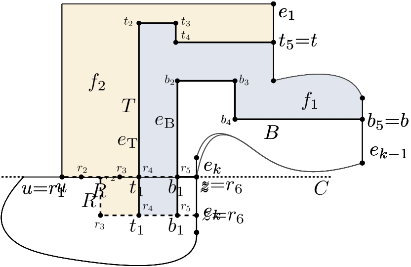
(a) $\Gamma_{1}$: $r_{2}r_{3}$ points right.

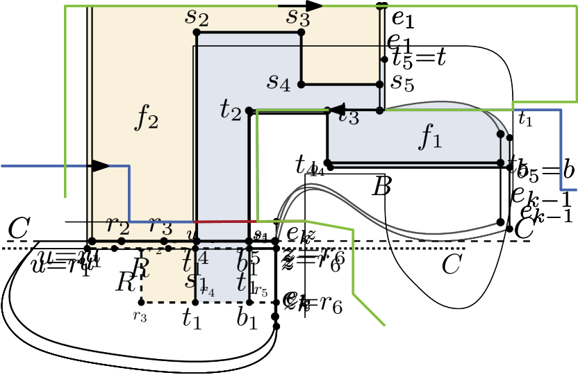
(b) $\Gamma_{1}$: $r_{2}r_{3}$ points downwards.

Figure 15: Illustration of Step 1, which inserts $R$, $T$ and $B$ into $\Gamma_{0}$. Depending on whether $uz$ lies on a horizontal cycle $C$ in $\Gamma_{0}$, the edge $r_{2}r_{3}$ points (15(a)) to the right or (15(b)) downwards.

5.2.2 Details of 2nd Improvement

We now describe the second phase of the augmentation step in greater detail. Let $u$ be the port that is currently considered by the augmentation step. In case that $u$ is a vertical port, we skip the second phase. So assume that $u$ is a horizontal port and that the first phase of the augmentation step inserts an edge $uz$ that points to the right; the case that $uz$ points to the left can be handled analogously by flipping the cylinder. We denote the resulting valid ortho-radial representation by $\Gamma_{0}$. Let $f$ be the face that locally lies to the left of $uz$. Further, let $e_{1},\dots,e_{k}$ be the candidate edges of $u$ that were considered before inserting $uz$, that is, the validity test failed for $e_{1},\dots,e_{k-1}$ and succeeded for $e_{k}$. If $k<4$ there are no intermediate candidates, and we skip the second phase. So assume that $k\geq 4$. We apply the following three steps to obtain the ortho-radial representations $\Gamma_{i}$ with $1\leq i\leq 3$. Later on, we show that each representation $\Gamma_{i}$ is valid, all intermediate candidates lie on rectangles in $\Gamma_{3}$, and there are only two more vertices becoming vertical ports and no more vertices becoming horizontal ports in $\Gamma_{3}$ than in $\Gamma_{0}$.

Step 1. We replace $uz$ by a structure consisting of three paths $R$, $T$, and $B$ as follows; see Figure 15 for an illustration. The path $R$ connects $u$ with $z$. It consists of six vertices $r_{i}$ with $1\leq i\leq 6$ such that $r_{1}=u$ and $r_{6}=z$. Apart from $r_{2}r_{3}$ all edges point to the right. For the direction of $r_{2}r_{3}$ we distinguish two cases. If $uz$ lies on a cycle whose labels are all $0$, the edge $r_{2}r_{3}$ points to the right and otherwise $r_{2}r_{3}$ points downwards; see Figure 15(15(a)) and (15(b)), respectively.

The path $T$ consists of five vertices $t_{i}$ with $1\leq i\leq 5$ such that $t_{1}=r_{4}$ and $t_{5}$ subdivides $e_{1}$. The edge $t_{1}t_{2}$ points upwards, the edge $t_{3}t_{4}$ points downwards, and the other two edges point to the right. Similarly, the path $B$ consists of five vertices $b_{i}$ with $1\leq i\leq 5$ such that $b_{1}=r_{5}$ and $b_{5}$ subdivides the edge $e_{k-1}$. Further, the edge $b_{1}b_{2}$ points upwards, the edge $b_{3}b_{4}$ points downwards, and the other two edges point to the right.

We denote the resulting ortho-radial representation by $\Gamma_{1}$. Further, let $f_{1}$ be the face that locally lies to the right of $T$, and let $f_{2}$ be the face that locally lies to the left of $T$.

Step 2. We iteratively resolve the ports in $f_{1}$ until the face is rectangulated. To that end, let $\Pi$ be the ortho-radial representation of the previous iteration; we start with $\Pi=\Gamma_{1}$. Further, let $u^{\prime}$ be the currently considered port of $f_{1}$ and let $e^{\prime}_{1},\dots,e^{\prime}_{l}$ be its candidates. If $u^{\prime}$ is a vertical port, we take $\Pi^{u^{\prime}}_{e^{\prime}_{1}}$ and otherwise $\Pi^{u^{\prime}}_{e^{\prime}_{l}}$ as result of the current iteration. The procedure stops when $f_{1}$ is completely rectangulated. We denote the resulting ortho-radial representation by $\Gamma_{2}$.

Step 3. Starting with $\Gamma_{2}$, we rectangulate the face $f_{2}$ by iteratively applying the augmentation step without Phase 2 until there are no ports left in $f_{2}$. We denote the resulting ortho-radial representation by $\Gamma_{3}$.

Correctness.

We now prove that the second phase yields a valid ortho-radial representation $\Gamma_{3}$ by showing that each step yields a valid ortho-radial representation. We use the same notation as above.

Step 1. In order to show the correctness, we successively add the paths $R$, $T$ and $B$ to $\Gamma_{0}$ and prove the validity of each created ortho-radial representation. To that end, let $\Gamma_{R}=\Gamma_{0}-uz+R$, $\Gamma_{T}=\Gamma_{R}+T$ and $\Gamma_{B}=\Gamma_{T}+B=\Gamma_{1}$.

Lemma 5.11.

The ortho-radial representation $\Gamma_{R}$ is valid.

Proof 5.12.

Assume that $\Gamma_{R}$ contains a monotone cycle $C$. Since $\Gamma_{0}$ is valid, this cycle uses $R$. In case that the edge $r_{2}r_{3}$ of $R$ points to the right, we can interpret $R$ as a single edge on $C$, because the labels of $C$ on $R$ are identical. Hence, $C$ corresponds to a cycle $C^{\prime}=C[z,u]+uz$ in $\Gamma_{0}$, where $uz$ is subdivided by some additional vertices on $C$. Thus, $C$ and $C^{\prime}$ have the same labels, which contradicts that $\Gamma_{0}$ is valid.

So assume that $r_{2}r_{3}$ points downwards. Without loss of generality, we assume that $C$ uses $uz$; the case that $C$ uses $zu$ can be handled identically. By construction the vertex $z$ is a newly introduced vertex subdividing $e_{k}$. Since $e_{k}$ is vertical, this implies that apart from $r_{2}r_{3}$ the cycle $C$ contains another vertical edge on $C[r_{6},r_{1}]$. Further, $C[r_{6},r_{1}]$ is also contained in $\Gamma_{0}$. Hence, $C[r_{6},r_{1}]+uz$ forms an essential cycle $C^{\prime}$ in $\Gamma_{0}$ with at least one vertical edge.

We show that for any common edge of $C$ and $C^{\prime}$ the labels of $C$ and $C^{\prime}$ are identical. Since all vertical edges of $C^{\prime}$ also belong to $C$, and $C^{\prime}$ has at least one vertical edge, this shows that $C^{\prime}$ is also monotone, which contradicts the validity of $\Gamma_{0}$.

Let $P$ be an elementary path to $C^{\prime}$ and let $v$ be the end vertex of $P$ on $C^{\prime}$. Since $uz$ belongs to $C^{\prime}$, the path does not contain this edge. Hence, $P$ is also contained in $\Gamma_{R}$ and it is an elementary path for $C$. Now consider an edge $e$ that belongs to both $C$ and $C^{\prime}$. Let $Q$ be the path on $C$ from $v$ to the target of $e$ and, analogously, let $Q^{\prime}$ be the path on $C^{\prime}$ from $v$ to the target of $e$. The path $Q$ contains $R$ if and only if $Q^{\prime}$ contains $uz$. Hence, if $Q$ does not contain $R$, both paths are identical, and we obtain

$$\ell_{C}(e)=\operatorname{rot}(e^{\star}+P+Q)=\operatorname{rot}(e^{\star}+P+Q^{\prime})=\ell_{C^{\prime}}(e).$$

So assume that $Q$ contains $R$. By construction we have $\operatorname{rot}(au+uz+zb)=\operatorname{rot}(au+R+zb)$, where $a$ is the vertex on $P+Q$ before $u$ and $b$ is the vertex on $Q$ after $z$. It holds

$$\ell_{C}(e) =\operatorname{rot}(e^{\star}+P+Q[v,u])+\operatorname{rot}(au+R+zb)+\operatorname{rot}(Q[zb,e])$$

$$=\operatorname{rot}(e^{\star}+P+Q^{\prime}[v,u])+\operatorname{rot}(au+uz+zb)+\operatorname{rot}(Q^{\prime}[zb,e])=\ell_{C^{\prime}}(e).$$

Hence, for common edges the labels of $C$ and $C^{\prime}$ are identical, which contradicts that $\Gamma_{0}$ is valid.

Next, we prove that $\Gamma_{T}$ is valid. To that end, we introduce the following definition. A cascading cycle is a non-monotone essential cycle that can be partitioned into two paths $P$ and $Q$ such that the labels on $P$ are $-1$ and the labels on $Q$ are non-negative. We further require that the edges incident to the internal vertices of $P$ either all lie in the interior of $C$ or they all lie in the exterior of $C$. In the first case we call $C$ an outer cascading cycle and in the second case an inner cascading cycle. The path $P$ is the negative path of the cycle.

To show that $\Gamma_{T}$ is valid, we construct a cascading cycle $C_{\mathrm{T}}$ in $\Gamma_{T}$ as follows. Let $C_{1}$ be the outermost decreasing cycle in $\Gamma^{u}_{e_{1}}$ and let $ut_{5}$ be the newly inserted edge in $\Gamma^{u}_{e_{1}}$. We replace $ut_{5}$ by $R[u,r_{4}]+T$ obtaining the cycle $C_{\mathrm{T}}$, which is well-defined because $C_{1}$ uses $ut_{5}$ in that direction by Lemma 5.1.

Lemma 5.13.

$C_{\mathrm{T}}$ is a cascading cycle no matter whether $r_{2}r_{3}$ points to the right or downwards. In particular, $t_{1}t_{2}$ is the negative path of $C_{\mathrm{T}}$.

Proof 5.14.

Let $C_{1}$ be the outermost decreasing cycle that in $\Gamma^{u}_{e_{1}}$ in the first phase. There is an elementary path $P$ from $e^{\star}$ that ends at a vertex $v$ on $C$. Since $P$ does not contain $ut_{5}$ in either direction, it is also an elementary path for $C_{\mathrm{T}}$ in $\Gamma_{T}$. Let further $Q$ be the path from $v$ to $u$. Since $C_{1}$ uses $ut_{5}$ in that direction, the path $Q$ does not use $ut_{5}$. This implies that $Q$ also exists on $C_{\mathrm{T}}$. Thus, $ut_{5}$ and $ur_{2}$ have the same label on $C_{1}$ and $C_{T}$. By Lemma 5.1 the edge $ut_{5}$ has label $0$ on $C_{1}$. If $r_{2}r_{3}$ points to the right the sequence of the labels on $R[u,r_{4}]+T$ is therefore $0$, $0$, $0$, $-1$, $0$, $1$, $0$. If $r_{2}r_{3}$ points downwards the sequence is $0$, $1$, $0$, $-1$, $0$, $1$, $0$. In both cases $C_{\mathrm{T}}$ is not monotone.

We now show that $t_{1}t_{2}$ is the only edge on $C_{\mathrm{T}}$ with negative label, which shows that $C_{\mathrm{T}}$ is a cascading cycle. In particular, the negative path consists of only one edge and therefore it has no internal vertices. We observe that $ut_{5}$ and $t_{4}t_{5}$ have the same label. Hence, for any common edge $e$ of $C_{1}$ and $C_{\mathrm{T}}$ there are paths $Q$ and $Q^{\prime}$ from $v$ to $e$, respectively, such that $\operatorname{rot}(e^{\star}+P+Q+e)=\operatorname{rot}(e^{\star}+P+Q^{\prime}+e)$. This implies that for any common edge of $C_{1}$ and $C_{\mathrm{T}}$, the labels of both cycles are identical. Since $C_{1}$ is a decreasing cycle, all common edges have non-negative labels. Altogether, $t_{1}t_{2}$ is the only edge of $C_{\mathrm{T}}$ with a negative label.

Using this lemma we prove that there is no decreasing cycle in $\Gamma_{T}$.

Lemma 5.15.

There is no decreasing cycle in $\Gamma_{T}$.

Proof 5.16.

Assume that $T$ is contained in a decreasing cycle $C$ (in either direction). Let $H=C+C_{\mathrm{T}}$ be the common sub-graph of $C$ and $C_{\mathrm{T}}$, and let $g$ be the central face of $H$. We distinguish the following two cases.

Case 1, $T$ is part of $g$. First assume that $C_{\mathrm{T}}$ and $C$ use $T$ in opposite directions. Since the central face locally lies to the right of any essential cycle, this implies that the central face lies to the left and right of $T$. Consequently, the central face is not simple, which contradicts that $H$ is biconnected. So assume that $C$ and $C_{\mathrm{T}}$ use $T$ in the same direction. By Proposition 2.2 it holds $\ell_{C_{\mathrm{T}}}(t_{1}t_{2})=\ell_{C}(t_{1}t_{2})$. Since the cycle $C_{\mathrm{T}}$ is a cascading cycle with negative path $t_{1}t_{2}$ by Lemma 5.13, it is $\ell_{C_{\mathrm{T}}}(t_{1}t_{2})=-1$. Thus, $C$ is not a decreasing cycle.

Case 2, $T$ is not part of $g$. Let $C^{\prime}$ be the essential cycle formed by $g$. Since $C^{\prime}$ consists of edges of $C$ and $C_{\mathrm{T}}$, the corresponding labels of $C$ and $C_{\mathrm{T}}$ also apply on $C^{\prime}$ by Proposition 2.2. Further, since $C$ is a decreasing cycle and $T$ is the only part of $C_{\mathrm{T}}$ that has a negative label on $C_{\mathrm{T}}$ by Lemma 5.13, the cycle $C^{\prime}$ only has non-negative labels. Since $T$ does not lie on $C^{\prime}$ but on $C_{\mathrm{T}}$, $C$ has at least one vertex with $C^{\prime}$ in common. This implies that $C^{\prime}$ has at least one positive label, because otherwise $C$ could not be a decreasing cycle by Proposition 2.3. Altogether, $C^{\prime}$ is a decreasing cycle that also exists in $\Gamma_{R}$, which contradicts its validity.

To show that $\Gamma_{T}$ contains no increasing cycle, we introduce a general lemma about the interaction of cascading and increasing cycles.

Lemma 5.17.

Let $C$ be a cascading cycle and $C^{\prime}$ an increasing cycle. Either $C$ lies in the interior of $C^{\prime}$ or vice versa.

Proof 5.18.

We assume without loss of generality that $C$ is an outer cascading cycle. The case that it is an inner cascading cycle can be handled by flipping the cylinder, which exchanges the exterior and interior of essential cycles but keeps the labels.

(a) The central face $g$.

(b) The labels are $-1$.

(c) The labels are $0$.

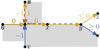
(d) $\ell_{C}(vw)=-1$ and $\ell_{C^{\prime}}(wx)=0$.

Figure 16: A common vertex $w$ on the central face $g$ of the subgraph formed by the cascading cycle $C$ and the increasing cycle $C^{\prime}$ and possible labels of the edges incident to $w$.

Let $g$ be the central face of the subgraph formed by the cycles $C$ and $C^{\prime}$. If $g$ is neither $C$ nor $C^{\prime}$, there are edges $vw$ and $wx$ on $g$ such that $vw$ lies on $C$ but not $C^{\prime}$, and $wx$ lies on $C^{\prime}$; see Figure 16(a). Let $uw$ be the edge on $C^{\prime}$ entering $w$. By construction, $uw$ lies strictly in the exterior of $g$. Hence, $vwx$ cannot make a left turn at $w$ and therefore $\ell_{g}(vw)\leq\ell_{g}(wx)$. Combining this with Proposition 2.2 and the bounds for the labels on $C$ and $C^{\prime}$ we get

$$-1\leq\ell_{C}(vw)=\ell_{g}(vw)\leq\ell_{g}(wx)=\ell_{C^{\prime}}(wx)\leq 0.$$

There are three cases for the labels $\ell_{C}(vw)$ and $\ell_{C^{\prime}}(wx)$: Either both are $-1$, both are $0$, or $\ell_{C}(vw)=-1$ and $\ell_{C^{\prime}}(wx)=0$.

If both labels are $-1$, the edge on $C$ after $w$ is $wx$; see Figure 16(b). It cannot be $wu$ because then the label of $wu$ would be $-2$. Hence, $w$ is an internal vertex of the negative path of $C$. But $uw$ lies in the exterior of $C$ contradicting that $C$ is an outer cascading cycle.

If both labels are $0$, the edge $uw$ must point down and therefore $\ell_{C^{\prime}}(uw)=1$, which contradicts that $C^{\prime}$ is increasing; see Figure 16(c).

Hence, $\ell_{C}(vw)=-1$ and $\ell_{C^{\prime}}(wx)=0$; see Figure 16(d). As before $uw$ cannot point down, which implies that it points right. The edge after $w$ on $C$ does not point left because it would have label $-2$. It does not point up since then $w$ would be an internal vertex of the negative path, and we get a contradiction as in the first case. Thus, $wx$ lies on $C$ and $w$ is the endpoint of the negative path $P$ of $C$. Therefore, there is a common path of $C$ and $C^{\prime}$ starting at $w$ and ending at a vertex $y$. Since $C$ is not monotone, it has an edge with a positive label and hence $y$ does not lie on $P$. Therefore, the edge on $C$ after $y$ has a non-negative label and the edge $yz$ on $C^{\prime}$ after $y$ has a non-positive label. By Lemma 13 in Reference [3], the edge $yz$ lies in the exterior of $C$. In total, this shows that no part of $C^{\prime}$ lies strictly in the interior of $C$ and therefore $g=C$.

Applying this lemma to the situation of $C_{\mathrm{T}}$ we prove that $\Gamma_{T}$ does not contain any increasing cycles. Together with Lemma 5.15 this yields that $\Gamma_{T}$ is valid.

Lemma 5.19.

There is no increasing cycle in $\Gamma_{T}$.

Proof 5.20.

Assume that $\Gamma_{T}$ contains an increasing cycle $C$, which uses $T$ in any direction. Lemma 5.17 implies that the central face $g$ of the subgraph formed by the two essential cycles $C$ and $C_{\mathrm{T}}$ is either $C$ or $C_{\mathrm{T}}$. In particular, $T$ or $\mkern 1.5mu\overline{\mkern-1.5muT\mkern-1.5mu}\mkern 1.5mu$ lies on $g$. Hence, both $C$ and $C_{\mathrm{T}}$ use $T$ in the same direction as otherwise $g$ would lie in the exterior of one of these cycles. But this would contradict that they are essential. Hence, they both contain $T$ in this direction and $T$ also lies on $g$. By Proposition 2.2 both cycles have the same labels on $T$. Since $\ell_{C_{\mathrm{T}}}(t_{1}t_{2})=-1$ by Lemma 5.13, we obtain $\ell_{C}(t_{3}t_{4})=\ell_{C_{\mathrm{T}}}(t_{3}t_{4})=1$. Consequently, $C$ is not an increasing cycle.

Hence, $\Gamma_{T}$ is valid. We analogously prove the validity of $\Gamma_{B}$ as for $\Gamma_{T}$. Let $C_{2}$ be the outermost decreasing cycle that in $\Gamma^{u}_{e_{k-1}}$ and let $ub_{5}$ be the newly inserted edge in $\Gamma^{u}_{e_{k-1}}$. We replace $ub_{5}$ by $R[u,r_{5}]+B$ obtaining the cycle $C_{\mathrm{B}}$, which is well-defined because $C_{2}$ uses $ub_{5}$ in that direction by Lemma 5.1.

Lemma 5.21.

$C_{\mathrm{B}}$ is a cascading cycles no matter whether $r_{2}r_{3}$ points to the right or downwards. In particular, $b_{1}b_{2}$ is the negative path of $C_{\mathrm{B}}$.

We omit the proof since it uses the same arguments as the proof of Lemma 5.13. Using similar arguments as in the proofs of Lemmas 5.15 and 5.19, we obtain that $\Gamma_{B}$ is valid.

Lemma 5.22.

The ortho-radial representation $\Gamma_{B}=\Gamma_{1}$ is valid.

Step 2. By Lemma 5.22 the ortho-radial representation $\Gamma_{1}$ of Step 1 is valid. We now prove that $\Gamma_{2}$ is a valid ortho-radial representation. We use the same notation as in the description of the algorithm.

Starting with the valid ortho-radial representation $\Gamma_{1}$, the procedure iteratively resolves ports in the face $f_{1}$, which locally lies to the right of $T$. In case that we resolve a vertical port $u^{\prime}$ in a representation $\Pi$, the resulting ortho-radial representation $\Pi^{u^{\prime}}_{e^{\prime}_{1}}$ is valid by Fact 1, where $e^{\prime}_{1}$ is the first candidate of $u^{\prime}$. So assume that $u^{\prime}$ is a horizontal port. In that case we take $\Pi^{u^{\prime}}_{e^{\prime}_{l}}$ for the next iteration, where $e^{\prime}_{l}$ is the last candidate of $u^{\prime}$. We observe that the augmentation of $f_{1}$ may subdivide edges on the negative paths of $C_{\mathrm{T}}$ and $C_{\mathrm{B}}$, but the added edges lie in the interior of $C_{\mathrm{T}}$ and the exterior of $C_{\mathrm{B}}$. Hence, $C_{\mathrm{T}}$ remains an outer cascading cycle and $C_{\mathrm{B}}$ an inner cascading cycle.

Lemma 5.23.

The ortho-radial representation $\Pi^{u^{\prime}}_{e^{\prime}_{l}}$ is valid.

Proof 5.24.

Assume that $\Pi^{u^{\prime}}_{e^{\prime}_{l}}$ is not valid. Hence, there is a monotone cycle $C$ that uses $e=u^{\prime}z^{\prime}$, where $z^{\prime}$ is the vertex subdividing $e^{\prime}_{l}$. Since $e^{\prime}_{l}$ is the last candidate of $u^{\prime}$, the cycle $C$ is increasing by Fact 2. By construction $e$ strictly lies in the interior of $C_{\mathrm{T}}$ and the exterior of $C_{\mathrm{B}}$. This implies that $C$ lies in the interior of $C_{\mathrm{T}}$ and the exterior of $C_{\mathrm{B}}$ by Lemma 5.17. In other words, $C$ is contained in the subgraph $H$ formed by the intersection of the interior of $C_{\mathrm{T}}$ and the exterior of $C_{\mathrm{B}}$. As $R[r_{1},r_{4}]$ belongs to both $C_{\mathrm{T}}$ and $C_{\mathrm{B}}$, it is incident to the outer and the central face of $H$. Hence, removing $R[r_{1},r_{4}]$ leaves a subgraph without essential cycles. Thus, the essential cycle $C$ includes $R[r_{1},r_{4}]$.

By Proposition 2.2 the labels of $C$ and $C_{\mathrm{T}}$ are the same on $R[r_{1},r_{4}]$. If $r_{2}r_{3}$ points downwards, its label is $1$, which contradicts that $C$ is increasing. If otherwise $r_{2}r_{3}$ points right, it lies on an essential cycle, where all labels are $0$. But then $C$ is not increasing by Proposition 2.3.

Altogether, applying the lemma inductively on the inserted edges, we obtain that $\Gamma_{2}$ is valid.

Step 3. As we only apply the first phase of the augmentation step on $f_{2}$, the resulting ortho-radial representation $\Gamma_{3}$ is also valid due to the correctness of the first phase. This concludes the correctness proof of the second phase.

Lemma 5.25.

The second phase produces a valid ortho-radial representation $\Gamma_{3}$ such that all intermediate candidates of $u$ lie on rectangles in $\Gamma_{3}$, and there are only two more vertices becoming vertical ports and no more vertices becoming horizontal ports in $\Gamma_{3}$ than in $\Gamma_{0}$.

Running Time.

We now prove that the rectangulation algorithm has $O(n^{2})$ running time in total. We first prove that the resulting ortho-radial representation has $O(n)$ vertices and edges, which implies that $O(n)$ augmentation steps are executed. Afterwards we show that the algorithm spends $O(n^{2})$ time in total for executing all augmentation steps.

Consider a single augmentation step that resolves a horizontal port $u$ of a face $f$. Let $K=B+T+R$ be the construction that is inserted during the second phase, and, furthermore, let $f_{1}$ and $f_{2}$ be the faces as defined above. After the second phase, only $r_{3}$ and $b_{4}$ of the newly inserted vertices have concave angles; all other concave angles of newly inserted vertices are resolved in the second phase by rectangulating $f_{1}$ and $f_{2}$. By construction both $r_{3}$ and $b_{4}$ can become vertical but not horizontal ports during the remaining procedure. Hence, we insert the construction $K$ only for vertices that already have existed in the input instance. Moreover, the rectangulation algorithm considers $O(n)$ vertical ports in total. Hence, the algorithm yields an ortho-radial representation with $O(n)$ vertices and edges. This also implies that $O(n)$ augmentation steps are executed.

In the remainder we show that the algorithm invests $O(n^{2})$ running time in total for the execution of all augmentation steps. In particular, we argue that the algorithm needs $O(n^{2})$ time for the computation of the candidates of all considered ports and all applied validity tests. Since the first and second phase of the augmentation step needs $O(1)$ time without considering the time necessary for the validity tests and the computation of the candidates, we finally obtain that the algorithm runs in $O(n^{2})$ time.

Since the rectangulation algorithm yields an ortho-radial representation with $O(n)$ vertices and edges, $O(n)$ ports are resolved and $O(n)$ different candidate edges are considered. Since the algorithm computes for each port its candidates only once (namely when the port is resolved), the algorithm spends $O(n^{2})$ time in total to compute all candidate edges of the ports.

We now bound the number of applied validity tests. Recall that we only apply validity tests in the first phase of the augmentation step and when rectangulating the face $f_{2}$ in the second phase. By Lemma 5.25 each edge can be an intermediate candidate for at most one vertex, which yields that there are $O(n)$ intermediate candidates over all augmentation steps. Finally, for each vertex there are at most three boundary candidates, which yields $O(n)$ boundary candidates over all augmentation steps. Assigning the validity tests to their candidates, we conclude that the algorithm executes $O(n)$ validity tests overall. Altogether, we obtain $O(n^{2})$ running time for the rectangulation algorithm.

In particular, using Corollary 19 from [3], given a graph $G$ with valid ortho-radial representation $\Gamma$, a corresponding ortho-radial drawing $\Delta$ can be computed in $O(n^{2})$ time.

6 Conclusion

In this paper, we have described an algorithm that checks the validity of an ortho-radial representation in $O(n^{2})$ time. In the positive case, we can also produce a corresponding drawing in the same running time, whereas in the negative case we find a monotone cycle. This answers an open question of Barth et al. [2] and allows for a purely combinatorial treatment of the bend minimization problem for ortho-radial drawings. It is an interesting open question whether the running time can be improved to near-linear. However, our main open question is how to find valid ortho-radial representations with few bends.

References

- [1] Md. Jawaherul Alam, Stephen G. Kobourov, and Debajyoti Mondal. Orthogonal layout with optimal face complexity. Computational Geometry, 63:40–52, 2017.
- [2] Lukas Barth, Benjamin Niedermann, Ignaz Rutter, and Matthias Wolf. Towards a Topology-Shape-Metrics Framework for Ortho-Radial Drawings. In Boris Aronov and Matthew J. Katz, editors, Computational Geometry (SoCG’17), volume 77 of Leibniz International Proceedings in Informatics (LIPIcs), pages 14:1–14:16. Schloss Dagstuhl–Leibniz-Zentrum fuer Informatik, 2017.
- [3] Lukas Barth, Benjamin Niedermann, Ignaz Rutter, and Matthias Wolf. Towards a topology-shape-metrics framework for ortho-radial drawings. CoRR, arXiv:1703.06040, 2017.
- [4] Carlo Batini, Enrico Nardelli, and Roberto Tamassia. A layout algorithm for data flow diagrams. IEEE Transactions on Software Engineering, SE-12(4):538–546, 1986.
- [5] P. Bertolazzi, G. Di Battista, and W. Didimo. Computing orthogonal drawings with the minimum number of bends. IEEE Transactions on Computers, 49(8):826–840, 2000.
- [6] Sandeep N. Bhatt and Frank Thomson Leighton. A framework for solving VLSI graph layout problems. Journal of Computer and System Sciences, 28(2):300–343, 1984.
- [7] Therese Biedl. New lower bounds for orthogonal graph drawings. In Franz J. Brandenburg, editor, Graph Drawing (GD’96), Lecture Notes of Computer Science, pages 28–39. Springer Berlin Heidelberg, 1996.
- [8] Therese Biedl and Goos Kant. A better heuristic for orthogonal graph drawings. Computational Geometry, 9(3):159 – 180, 1998.
- [9] Therese C. Biedl, Brendan P. Madden, and Ioannis G. Tollis. The three-phase method: A unified approach to orthogonal graph drawing. In Giuseppe DiBattista, editor, Graph Drawing (GD’97), Lecture Notes in Computer Science, pages 391–402. Springer Berlin Heidelberg, 1997.
- [10] Thomas Bläsius, Ignaz Rutter, and Dorothea Wagner. Optimal orthogonal graph drawing with convex bend costs. ACM Transactions on Algorithms, 12(3):33, 2016.
- [11] Thomas Bläsius, Sebastian Lehmann, and Ignaz Rutter. Orthogonal graph drawing with inflexible edges. Computational Geometry, 55:26 – 40, 2016.
- [12] Yi-Jun Chang and Hsu-Chun Yen. On bend-minimized orthogonal drawings of planar 3-graphs. In Boris Aronov and Matthew J. Katz, editors, Computational Geometry (SoCG’17), volume 77 of Leibniz International Proceedings in Informatics (LIPIcs). Schloss Dagstuhl-Leibniz-Zentrum fuer Informatik, 2017.
- [13] Sabine Cornelsen and Andreas Karrenbauer. Accelerated bend minimization. In Marc van Kreveld and Bettina Speckmann, editors, Graph Drawing (GD’12), Lecture Notes of Computer Science, pages 111–122. Springer Berlin Heidelberg, 2012.
- [14] Markus Eiglsperger, Carsten Gutwenger, Michael Kaufmann, Joachim Kupke, Michael Jünger, Sebastian Leipert, Karsten Klein, Petra Mutzel, and Martin Siebenhaller. Automatic layout of uml class diagrams in orthogonal style. Information Visualization, 3(3):189–208, 2004.
- [15] Markus Eiglsperger, Michael Kaufmann, and Martin Siebenhaller. A topology-shape-metrics approach for the automatic layout of uml class diagrams. In Software Visualization (SoftVis’03), pages 189–ff. ACM, 2003.
- [16] Stefan Felsner, Michael Kaufmann, and Pavel Valtr. Bend-optimal orthogonal graph drawing in the general position model. Computational Geometry, 47(3, Part B):460–468, 2014. Special Issue on the 28th European Workshop on Computational Geometry (EuroCG 2012).
- [17] Martin Fink, Herman Haverkort, Martin Nöllenburg, Maxwell Roberts, Julian Schuhmann, and Alexander Wolff. Drawing metro maps using bézier curves. In W Didimo and M Patrignani, editors, Graph Drawing (GD’13), Lecture Notes in Computer Science, pages 463–474. Springer International Publishing, 2013.
- [18] Ulrich Fößmeier and Michael Kaufmann. Drawing high degree graphs with low bend numbers. In Franz J. Brandenburg, editor, Graph Drawing (GD’96), Lecture Notes in Computer Science, pages 254–266. Springer Berlin Heidelberg, 1996.
- [19] Carsten Gutwenger, Michael Jünger, Karsten Klein, Joachim Kupke, Sebastian Leipert, and Petra Mutzel. A new approach for visualizing UML class diagrams. In Symposium on Software Visualization (SoftVis’03), pages 179–188, New York, NY, USA, 2003. ACM.
- [20] Madieh Hasheminezhad, S. Mehdi Hashemi, Brendan D. McKay, and Maryam Tahmasbi. Rectangular-radial drawings of cubic plane graphs. Computational Geometry: Theory and Applications, 43:767–780, 2010.
- [21] Madieh Hasheminezhad, S. Mehdi Hashemi, and Maryam Tahmasbi. Ortho-radial drawings of graphs. Australasian Journal of Combinatorics, 44:171–182, 2009.
- [22] Seok-Hee Hong, Damian Merrick, and Hugo A. D. do Nascimento. Automatic visualisation of metro maps. Journal of Visual Languages and Computing, 17(3):203–224, 2006.
- [23] S. Kieffer, T. Dwyer, K. Marriott, and M. Wybrow. Hola: Human-like orthogonal network layout. IEEE Transactions on Visualization and Computer Graphics, 22(1):349–358, 2016.
- [24] Martin Nöllenburg and Alexander Wolff. Drawing and labeling high-quality metro maps by mixed-integer programming. Transactions on Visualization and Computer Graphics, 17(5):626–641, 2011.
- [25] Achilleas Papakostas and Ioannis G. Tollis. Algorithms for area-efficient orthogonal drawings. Computational Geometry, 9(1):83–110, 1998.
- [26] Ulf Rüegg, Steve Kieffer, Tim Dwyer, Kim Marriott, and Michael Wybrow. Stress-minimizing orthogonal layout of data flow diagrams with ports. In Christian Duncan and Antonios Symvonis, editors, Graph Drawing (GD’14), Lecture Notes in Computer Science, pages 319–330. Springer Berlin Heidelberg, 2014.
- [27] R. Tamassia. On embedding a graph in the grid with the minimum number of bends. Journal on Computing, 16(3):421–444, 1987.
- [28] Roberto Tamassia, Giuseppe Di Battista, and Carlo Batini. Automatic graph drawing and readability of diagrams. IEEE Transactions on Systems, Man, and Cybernetics, 18(1):61–79, 1988.
- [29] Roberto Tamassia, Ioannis G. Tollis, and Jeffrey Scott Vitter. Lower bounds for planar orthogonal drawings of graphs. Information Processing Letters, 39(1):35 – 40, 1991.
- [30] L. G. Valiant. Universality considerations in vlsi circuits. IEEE Transactions on Computers, 30(02):135–140, 1981.
- [31] Yu-Shuen Wang and Ming-Te Chi. Focus+context metro maps. Transactions on Visualization and Computer Graphics, 17(12):2528–2535, 2011.
- [32] Michael Wybrow, Kim Marriott, and Peter J. Stuckey. Orthogonal connector routing. In David Eppstein and Emden R. Gansner, editors, Graph Drawing (GD’10), Lecture Notes in Computer Science, pages 219–231. Springer Berlin Heidelberg, 2010.