The All-or-Nothing Phenomenon in Sparse Linear Regression

Abstract

We study the problem of recovering a hidden binary $k$-sparse $p$-dimensional vector $\beta$ from $n$ noisy linear observations $Y=X\beta+W$ where $X_{ij}$ are i.i.d.  $\mathcal{N}(0,1)$ and $W_{i}$ are i.i.d.  $\mathcal{N}(0,\sigma^{2})$. A closely related hypothesis testing problem is to distinguish the pair $(X,Y)$ generated from this structured model from a corresponding null model where $(X,Y)$ consist of purely independent Gaussian entries. In the low sparsity $k=o(p)$ and high signal to noise ratio $k/\sigma^{2}=\Omega\left(1\right)$ regime, we establish an “All-or-Nothing” information-theoretic phase transition at a critical sample size $n^{*}=2k\log\left(p/k\right)/\log\left(1+k/\sigma^{2}\right)$, resolving a conjecture of [GZ17a]. Specifically, we show that if $\liminf_{p\to\infty}n/n^{*}>1$, then the maximum likelihood estimator almost perfectly recovers the hidden vector with high probability and moreover the true hypothesis can be detected with a vanishing error probability. Conversely, if $\limsup_{p\to\infty}n/n^{*}<1$, then it becomes information-theoretically impossible even to recover an arbitrarily small but fixed fraction of the hidden vector support, or to test hypotheses strictly better than random guess.

Our proof of the impossibility result builds upon two key techniques, which could be of independent interest. First, we use a conditional second moment method to upper bound the Kullback-Leibler (KL) divergence between the structured and the null model. Second, inspired by the celebrated area theorem, we establish a lower bound to the minimum mean squared estimation error of the hidden vector in terms of the KL divergence between the two models.

1 Introduction

In this paper, we study the information-theoretic limits of the Gaussian sparse linear regression problem. Specifically, for $n,p,k\in\mathbb{N}$ with $k\leq p$ and $\sigma^{2}>0$ we consider two independent matrices $X\in{\mathbb{R}}^{n\times p}$ and $W\in{\mathbb{R}}^{n\times 1}$ with $X_{ij}{\stackrel{{\scriptstyle\text{i.i.d.}}}{{\sim}}}{\mathcal{N}}(0,1)$ and $W_{i}{\stackrel{{\scriptstyle\text{i.i.d.}}}{{\sim}}}{\mathcal{N}}(0,\sigma^{2})$, and observe

$$Y=X\beta+W,$$ (1)

where $\beta$ is assumed to be uniformly chosen at random from the set $\{v\in\{0,1\}^{p}:\|v\|_{0}=k\}$ and independent of $(X,W)$. The problem of interest is to recover $\beta$ given the knowledge of $X$ and $Y$. Our focus will be on identifying the minimal sample size $n$ for which the recovery is information-theoretic possible.

The problem of recovering the support of a hidden sparse vector $\beta\in\mathbb{R}^{p}$ given noisy linear observations has been extensively analyzed in the literature, as it naturally arises in many contexts including subset regression, e.g. [CH90], signal denoising, e.g. [CDS01], compressive sensing, e.g. [CT05], [Don06], information and coding theory, e.g. [JB12], as well as high dimensional statistics, e.g. [Wai09a, Wai09b]. The assumptions of Gaussianity of the entries of $(X,W)$ are standard in the literature. Furthermore, much of the literature (e.g. [ASZ10], [NT18], [WWR10]) assumes a lower bound $\beta_{\min}>0$ for the smallest magnitude of a nonzero entry of $\beta$, that is $\min_{i:\beta_{i}\not=0}|\beta_{i}|\geq\beta_{\min}$, as otherwise identification of the support of the hidden vector is in principle impossible. In this paper we adopt a simplifying assumption by focusing only on binary vectors $\beta$, similar to other papers in the literature such as [ASZ10], [GZ17a] and [GZ17b]. In this case recovering the support of the vectors is equivalent to identifying the vector itself.

To judge the recovery performance we focus on the mean squared error (MSE). That is, given an estimator $\widehat{\beta}$ as a function of $(X,Y)$, define mean squared error as

$$\text{MSE}\left(\widehat{\beta}\right)\triangleq\mathbb{E}\left[\|\widehat{\beta}-\beta\|^{2}\right],$$

where $\|v\|$ denotes the $\ell_{2}$ norm of a vector $v$. In our setting, one can simply choose $\widehat{\beta}=\mathbb{E}\left[\beta\right]$, which equals $\frac{k}{p}(1,1,\ldots,1)^{\top}$, and obtain a trivial $\text{MSE}_{0}=\mathbb{E}\left[\|\beta-\mathbb{E}\left[\beta\right]\|^{2}\right]$, which equals $k\left(1-\frac{k}{p}\right)$. We will adopt the following two natural notions of recovery, by comparing the MSE of an estimator $\widehat{\beta}$ to $\text{MSE}_{0}$.

Definition 1 (Strong and weak recovery).

We say that $\widehat{\beta}=\widehat{\beta}(Y,X)\in\mathbb{R}^{p}$ achieves

• strong recovery if $\limsup_{p\to\infty}\text{MSE}\left(\widehat{\beta}\right)/\text{MSE}_{0}=0$;

• weak recovery if $\limsup_{p\to\infty}\text{MSE}\left(\widehat{\beta}\right)/\text{MSE}_{0}<1.$

The fundamental question of interest in this paper is when $n$ as a function of $(p,k,\sigma^{2})$ is such that strong/weak recovery is information-theoretically possible.

The focus of this paper will be on sublinear sparsity levels, that is on $k=o\left(p\right)$. A great amount of literature has been devoted on the study of the problem in the linear regime where $n,k,\sigma=\Theta(p).$ One line of work has provided upper and lower bounds on the accuracy of support recovery as a function of the problem parameters, e.g. [ASZ10, RG12, RG13, SC17]. Another line of work has derived explicit formulas for the minimum MSE (MMSE) $\mathbb{E}\left[\|\beta-\mathbb{E}\left[\beta\mid X,Y\right]\|^{2}\right]$. These formulas were first obtained heuristically using the replica method from statistical physics [Tan02, GV05] and later proven rigorously in [RP16, BDMK16]. However, to our best of knowledge, none of the rigorous techniques of [RP16, BDMK16] apply when $k=o(p)$. Although there has been significant work focusing directly on the sublinear sparsity regime, the identification of the exact information theoretic threshold of this fundamental statistical problem remains largely open (see Section 1.2 for a detailed discussion).

Obtaining a tight characterization of the information-theoretic threshold is the main contribution of this work.

Towards identifying the information theoretic limits of recovering $\beta$, and out of independent interest, we also consider a closely related hypothesis testing problem, where the goal is to distinguish the pair $(X,Y)$ generated according to (1) from a model where both $X$ and $Y$ are independently generated. More specifically, given two independent matrices $X\in{\mathbb{R}}^{n\times p}$ and $W\in{\mathbb{R}}^{n\times 1}$ with $X_{ij}{\stackrel{{\scriptstyle\text{i.i.d.}}}{{\sim}}}{\mathcal{N}}(0,1)$ and $W_{i}{\stackrel{{\scriptstyle\text{i.i.d.}}}{{\sim}}}{\mathcal{N}}(0,\sigma^{2})$, we define

$$Y\triangleq\lambda W,$$ (2)

where $\lambda>0$ is a scaling parameter. We refer to the Gaussian linear regression model (1) as the planted model, denoted by $P=P(X,Y)$, and (2) as the null model denoted by $Q_{\lambda}=Q_{\lambda}(Y,X)$. We focus on characterizing the total variation distance $\mathrm{TV}\left(P,Q_{\lambda}\right)$ for various values of $\lambda$. One choice of particular interest is $\lambda=\sqrt{k/\sigma^{2}+1}$, under which $\mathbb{E}\left[YY^{\top}\right]=(k+\sigma^{2})\mathbf{I}$ in both the planted and null models.

Analogous to recovery, we adopt the following two natural notions of testing [PWB16, AKJ17].

Definition 2 (Strong and weak detection).

Fix two probability measures $\mathbb{P},\mathbb{Q}$ on our observed data $(Y,X)$. We say a test statistic ${\mathcal{T}}(X,Y)$ with a threshold $\tau$ achieves

• strong detection if

  $$\limsup_{p\to\infty}\left[\mathbb{P}({\mathcal{T}}(X,Y)<\tau)+\mathbb{Q}({\mathcal{T}}(X,Y)\geq\tau)\right]=0,$$

• weak detection, if

  $$\limsup_{p\to\infty}[\mathbb{P}({\mathcal{T}}(X,Y)<\tau)+\mathbb{Q}({\mathcal{T}}(X,Y)\geq\tau)]<1.$$

Note that strong detection asks for the test statistic to determine with high probability whether $(X,Y)$ is drawn from $\mathbb{P}$ or $\mathbb{Q}$, while weak detection, similar to weak recovery, only asks for the test statistic to strictly outperform the random guess. Recall that

$$\inf_{{\mathcal{T}},\tau}\left[\mathbb{P}({\mathcal{T}}(X,Y)<\tau)+\mathbb{Q}({\mathcal{T}}(X,Y)\geq\tau)\right]=1-\mathrm{TV}(P,Q).$$

Thus equivalently, strong detection is possible if and only if $\liminf_{p\to\infty}\mathrm{TV}(\mathbb{P},\mathbb{Q})=1$, and weak detection is possible if and only if $\liminf_{p\to\infty}\mathrm{TV}(\mathbb{P},\mathbb{Q})>0.$ The fundamental question of interest is when $n$ as a function of $(p,k,\sigma^{2})$ is such that strong/weak detection is information-theoretically possible.

1.1 Contributions

Of fundamental importance is the following sample size:

$$n^{*}\triangleq\frac{2k\log(p/k)}{\log(1+k/\sigma^{2})}.$$ (3)

We establish that $n^{*}$ is a sharp phase transition point for the recovery of $\beta$ when $k=o(\sqrt{p})$ and the signal to noise ratio $k/\sigma^{2}$ is above a sufficiently large constant. In particular, for an arbitrarily small but fixed constant $\epsilon>0$, when $n<(1-\epsilon)n^{*}$, weak recovery is impossible, but when $n>(1+\epsilon)n^{*}$, strong recovery is possible. This implies that the rescaled MMSE undergoes a jump from $1$ to $0$ at $n^{*}$ samples up to a small window of size $\epsilon n$.

We state this in the following Theorem, which summarizes the Theorems 2, 3, 4 and 5 from the main body of the paper.

Theorem (All-or-Nothing Phase Transition).

Let $\delta\in(0,\frac{1}{2})$ and $\epsilon\in(0,1)$ be two arbitrary but fixed constants. Then there exists a constant $C(\delta,\epsilon)>0$ only depending only $\delta$ and $\epsilon$, such that if $k/\sigma^{2}\geq C(\delta,\epsilon)$, then

• When $k\leq p^{\frac{1}{2}-\delta}$ and

  $$n<\left(1-\epsilon\right)n^{*},$$

  both weak recovery of $\beta$ from $(Y,X)\sim P$ and weak detection between $P$ and $Q_{\lambda_{0}}$ are information-theoretically impossible, where $\lambda_{0}=\sqrt{\frac{k}{\sigma^{2}}+1}$.

• When $k=o(p)$ and

  $$n>\left(1+\epsilon\right)n^{*},$$

  both strong recovery of $\beta$ from $(Y,X)\sim P$ and $(\dagger)$ strong detection between $P$ and $Q_{\lambda}$ are information-theoretically possible for any $\lambda>0$.

  $(\dagger)$: strong detection requires an additional assumption $1+k/\sigma^{2}\leq\left(k\log\left(p/k\right)\right)^{1-\eta}$ for some arbitrarily small but fixed constant $\eta>0.$

Note that the theorem above assumes $\sigma>0$. In the extreme case where $\sigma=0$, $n^{*}$ trivializes to zero and we can directly argue that one sample suffices for strong recovery. In fact, for any $\beta\in\{0,1\}^{p}$ and $Y_{1}=\langle X_{1},\beta\rangle$ for $X_{1}\sim\mathcal{N}(0,\mathbf{I}_{p})$, we can identify $\beta$ as the unique binary-valued solution of $Y_{1}=\langle X_{1},\beta\rangle$, almost surely with respect to the randomness of $X$ (see e.g. [GZ18])

Note that the first part of the above result focuses on $k\leq p^{1/2-\delta}$. It turns out that this is not a technical artifact and $k=o\left(p^{1/2}\right)$ is needed for $n^{*}$ to be the weak detection sample size threshold. More details can be found in Appendix C. The sharp information-theoretic threshold for either detection or recovery is still open when $k=\Omega\left(p^{1/2}\right)$ and $k=o(p)$.

The phase transition role of $n^{*}$

According to our main result, the rescaled minimum mean squared error of the problem, $\mathrm{MMSE}/\text{MSE}_{0}$, exhibits a step behavior asymptotically. Loosely speaking, when $n<n^{*}$ it equals to one and when $n>n^{*}$ it equals to zero. We next intuitively explain why such a step behavior for sparse high dimensional regression occurs at $n^{*}$, using ideas related to the area theorem. The area theorem has been used in the channel coding literature to study the MAP decoding threshold [MMU08] and the capacity-achieving codes [KKM⁺17]. The approach described below is similar to the one used previously for linear regression [RP16].

First let us observe that $n^{*}$ is asymptotically equal to the ratio of entropy $H(\beta)=\log\binom{p}{k}$ and Gaussian channel capacity $\frac{1}{2}\log(1+k/\sigma^{2})$. We explore this coincidence in the following way. Let $I_{n}\triangleq I(Y_{1}^{n};X,\beta)$ denote the mutual information between $\beta$ and $(Y_{1}^{n};X)$ with a total of $n$ linear measurements. Since the mutual information in the Gaussian channel under a second moment constraint is maximized by the Gaussian input distribution, it follows that the increment of mutual information $I_{n+1}-I_{n}\leq\frac{1}{2}\log(1+\mathrm{MMSE}_{n}/\sigma^{2})$, where $\mathrm{MMSE}_{n}$ denotes the minimum MSE with $n$ measurements. In particular, all the increments are between zero and $\frac{1}{2}\log(1+k/\sigma^{2})$ and by telescopic summation for any $n$:

$$I_{n}\leq\frac{n}{2}\log(1+k/\sigma^{2}),$$ (4)

with equality only if for all $m<n$, $\mathrm{MMSE}_{m}=k$. This is illustrated in Fig. 1 where we plot $n$ against $I_{n+1}-I_{n}$.

Suppose now that we have established that strong recovery is achieved with $n^{*}=\frac{H(\beta)}{\frac{1}{2}\log(1+k/\sigma^{2})}$ samples.

Then strong recovery and standard identities connecting mutual information and entropy implies that

$$I_{n^{*}}=H(\beta)=\frac{n^{*}}{2}\log(1+k/\sigma^{2}).$$

In particular, (4) holds with equality, which means for all $n\leq n^{*}-1$, $\mathrm{MMSE}_{n}=k$. In particular, for all $n<n^{*}$, weak recovery is impossible. This area theorem is the key underpinning our converse proof of the weak recovery.

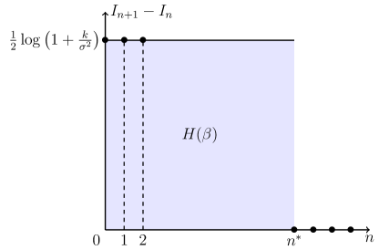
Figure 1: The phase transition diagram in Gaussian sparse linear regression. The $y$-axis is the increment of mutual information with one additional measurement. The area of blue region equals the entropy $H(\beta)\sim k\log(p/k)$.

1.2 Comparison with Related Work

The information-theoretic limits of high-dimensional sparse linear regression have been studied extensively and there is a vast literature of multiple decades of research. In this section we focus solely on the Gaussian and binary setting and furthermore on the results applying to high values of signal to noise ratio and sublinear sparsity.

Information-theoretic Negative Results for weak/strong recovery

For the impossibility direction, previous work [ASZ10, Theorem 5.2] has established that as $p\to\infty$, achieving $\mathrm{MSE}(\widehat{\beta})\leq d$ for any $d\in[0,k]$ is information-theoretically impossible if

$$n\leq 2p\frac{h_{2}(k/p)-h_{2}(d/p)}{\log\left(1+k/\sigma^{2}\right)},$$

where $h_{2}(\alpha)=-\alpha\log\alpha-(1-\alpha)\log(1-\alpha)$ for $\alpha\in[0,1]$ is the binary entropy function. This converse result is proved via a simple rate-distortion argument (see, e.g. [WX18] for an exposition). In particular, given any estimator $\widehat{\beta}(X,Y)$ with $\text{MSE}(\widehat{\beta})\leq d$, we have

$$p\left(h_{2}(k/p)-h_{2}(d/p)\right)\leq\inf_{\text{MSE}(\widetilde{\beta})\leq d}I(\widetilde{\beta};\beta)\leq I(\widehat{\beta};\beta)\leq I(X,Y;\beta)\leq\frac{n}{2}\log\left(1+k/\sigma^{2}\right).$$

Notice that since $k=o(p)$ the result implies that if $n\leq\left(1-o\left(1\right)\right)n^{*}$, strong recovery, that is $d=o(k)$, is information-theoretically impossible and if $n=o(n^{*})$, weak recovery, that is $d\leq(1-\epsilon)k$ for an arbitrary $\epsilon\in(0,1)$, is impossible.

More recent work [SC17, Corollary 2] further quantified the fraction of support that can be recovered when $n<(1-\epsilon)n^{*}$ for some fixed constant $\epsilon>0$. Specifically with $k=o(p)$ and any scaling of $k/\sigma^{2}$, if $n<(1-\epsilon)n^{*}$, then the fraction of the support of $\beta$ that can be recovered correctly is at most $1-\epsilon$ with high probability; thus strong recovery is impossible.

Restricting to the Maximum Likelihood Estimator (MLE) performance of the problem, it is shown in [GZ17a] that under significantly small sparsity $k=O\left(\exp\left(\sqrt{\log p}\right)\right)$ and $k/\sigma^{2}\rightarrow+\infty$, if $n\leq(1-\epsilon)n^{*}$, the MLE not only fails to achieve strong recovery, but also fails to weakly recover the vector, that is recover correctly any positive constant fraction of the support.

Our result (Theorem 3) establishes that the MLE performance is fundamental. It improves upon the negative results in the literature by identifying a sharp threshold for weak recovery, showing that if $k=o\left(\sqrt{p}\right)$, $k/\sigma^{2}\geq C$ for some large constant $C>0$, and $n\leq\left(1-\epsilon\right)n^{*}$, then weak recovery is information-theoretically impossible by any estimator $\widehat{\beta}(Y,X)$. In other words, no constant fraction of the support is recoverable under these assumptions.

Information-theoretic Positive Results for weak/strong recovery

In the positive direction, previous work [AT10, Theorem 1.5] shows that when $k=o(p)$, $k/\sigma^{2}=\Theta(1)$, and $n>C_{k/\sigma^{2}}k\log(p-k)$ for some $C_{k/\sigma^{2}}$, it is information theoretically possible to weakly recover the hidden vector.

Albeit very similar to our results, our positive result (Theorem 4) identifies the explicit value of $C_{k/\sigma^{2}}$ for which both weak and strong recovery are possible, that is $C_{k/\sigma^{2}}=2/\log\left(1+k/\sigma^{2}\right)$ for which $C_{k/\sigma^{2}}k\log(p/k)=n^{*}$.

In [GZ17a] it is shown that when $k=O\left(\exp\left(\sqrt{\log p}\right)\right)$ and $k/\sigma^{2}\rightarrow+\infty$ then if $n\geq(1+\epsilon)n^{*}$ for some fixed $\epsilon>0$, strong recovery is achieved by the MLE of the problem. We improve upon this result with Theorem 4 by showing that when $n\geq(1+\epsilon)n^{*}$ for some fixed $\epsilon>0$ and any $k\leq cp$ for some $c>0$, then there exists a constant $C>0$ such that $k/\sigma^{2}\geq C$ the MLE achieves strong recovery. In particular, we significantly relax the assumption from [GZ17a] by showing that MLE achieves strong recovery with $(1+\epsilon)n^{*}$ samples for (1) any sparsity level less than $cp$ and (2) finite but large values of signal to noise ratio.

Exact asymptotic characterization of MMSE for linear sparsity

For both weak and strong recovery, the central object of interest is the MMSE $\mathbb{E}\left[\|\beta-\mathbb{E}\left[\beta\mid X,Y\right]\|^{2}\right]$ and its asymptotic behavior. While the asymptotic behavior of the MMSE remains a challenging open problem when $k=o(p)$, it has been accurately understood when $k=\Theta(p)$ and $k/\sigma^{2}=\Theta(1)$.

To be more specific, consider the asymptotic regime where $k=\varepsilon p$, $\sigma^{2}=k/\gamma$, and $n=\delta p$, for fixed positive constants $\varepsilon,\gamma,\delta$ as $p\to+\infty$. The asymptotic minimum mean-square error (MMSE) can be characterized explicitly in terms of $(\varepsilon,\gamma,\delta)$.

This characterization was first obtained heuristically using the replica method from statistical physics [Tan02, GV05] and later proven rigorously [RP16, BDMK16]. More specifically, for fixed $(\varepsilon,\gamma)$, let the asymptotic MMSE as a function of $\delta$ be defined by

$$\mathcal{M}_{\varepsilon,\gamma}(\delta)=\lim_{p\to\infty}\frac{\mathbb{E}\left[\|\beta-\mathbb{E}\left[\beta\mid X,Y\right]\|^{2}\right]}{\mathbb{E}\left[\|\beta-\mathbb{E}\left[\beta\right]\|^{2}\right]}.$$

The results in [RP16, BDMK16] lead to an explicit formula for $\mathcal{M}_{\varepsilon,\gamma}(\delta)$. Furthermore, they show that for $\varepsilon\in(0,1)$ and all sufficiently large $\gamma\in(0,\infty)$, $\mathcal{M}_{\varepsilon,\gamma}(\delta)$ has a jump discontinuity as a function of $\delta$. The location of this discontinuity, denoted by $\delta^{*}=\delta^{*}(\varepsilon,\gamma)$, occurs at a value that is strictly greater than the threshold $n^{*}/p$.

Furthermore, at the the discontinuity, the MMSE transitions from a value that is strictly less than the MMSE without any observations to a value that is strictly positive, i.e., $\mathcal{M_{\varepsilon,\gamma}}(0)>\lim_{\delta\uparrow\delta^{*}}\mathcal{M}_{\varepsilon,\gamma}(\delta)>\lim_{\delta\downarrow\delta^{*}}\mathcal{M}_{\varepsilon,\gamma}(\delta)>0$.

To compare these formulas to the sub-linear sparsity studied in this paper, one can consider the limiting behavior of $\mathcal{M}_{\varepsilon,\gamma}(\delta)$ as $\varepsilon$ decreases to zero. It can be verified that $\mathcal{M}_{\varepsilon,\gamma}(\delta)$ converges indeed to a step zero-one function as $\varepsilon\to 0$ and the jump discontinuity transfers indeed to the critical value $n^{*}/p$ which makes the behavior consistent with the results in this paper.

However, an important difference is that the results in this paper are derived directly under the scaling regime $k=o(p)$ whereas the derivation described above requires one to first take the asymptotic limit $p\to\infty$ for fixed $(\epsilon,\gamma)$ and then take $\epsilon\to 0$. Since the limits cannot interchange in any obvious way, the results in this paper cannot be derived as a consequence of the rigorous results in [RP16, BDMK16]. Finally, it should be mentioned that taking the limit $\epsilon\to 0$ for the replica prediction suggests the step behavior for all values of signal-to-noise ratio $\gamma$ (see Figure 2). In this paper, the step behavior is rigorously proven in the high signal-to-noise ratio regime. The proof of the step behavior when the signal-to-noise ratio is low remains an open problem.

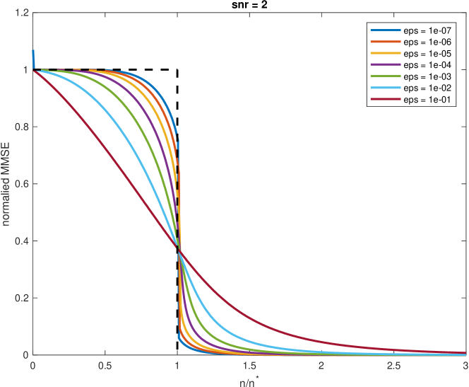
Figure 2: The limit of the replica-symmetric predicted MMSE $\mathcal{M}_{\varepsilon,\gamma}(\cdot)$ as $\epsilon\to 0$ for signal to noise ratio (snr) $\gamma$ equal to $2$ (left curve) and equal to $10$ (right curve).

Sparse Superposition Codes

Constructing an algorithm for recovering a binary $k$-sparse $\beta$ from $(Y=X\beta+W,X)$ receives a lot of attention from a coding theory point of view. The reason is that such recovery corresponds naturally to a code for the memoryless additive Gaussian white noise (AWGN) channel with signal-to-noise ratio equal to $k/\sigma^{2}$. Specifically in this context achieving strong recovery of a uniformly chosen binary $k$-sparse $\beta$ with $(1+\epsilon)n^{*}$ samples, for arbitrary $\epsilon>0$, corresponds exactly to capacity-achieving encoding-decoding mechanism of $\binom{p}{k}\sim(pe/k)^{k}$ messages through a AWGN channel. A recent line of work has analyzed a similar mechanism where $(p/k)^{k}$ messages are encoded through $k$-block-sparse vectors; that is the vector $\beta$ is designed to have at most one non-zero value in each of $k$ block of entries indexed by $i\lfloor p/k\rfloor,i\lfloor p/k\rfloor+1,\cdots,(i+1)\lfloor p/k\rfloor-1$ for $i=0,1,2,\ldots,k-1$. It has shown that by using various polynomial-time decoding mechanisms, such as adaptive successive decoding [JB12], [JB14], a soft-decision iterative decoder [BC12], [Cho14] and finally Approximate Message Passing techniques [RGV17], one can strongly recover the hidden $k$-block-sparse vector with $(1+\epsilon)n^{*}$ samples and achieve capacity. Their techniques are tailored to work for any $k=p^{1-c}$ with $c\in(0,1)$ and also require the vector to have carefully chosen non-zero entries, that is the hidden vector is not assumed to simply be binary. In this work Theorem 4 establishes that under the simple assumption on $\beta$ being binary and arbitrarily (not block) $k$-sparse it suffices to make strong recovery possible with $(1+\epsilon)n^{*}$ samples when $k=o(p)$. Nevertheless, our decoding mechanism requires a search over the space of $k$-sparse binary vectors and therefore is not in principle polynomial-time. The design of a polynomial-time recovery algorithm for this task and $(1+\epsilon)n^{*}$ samples remains largely an open problem (see [GZ17a]).

Information-theoretic limits up to constant factors for exact recovery

Although exact recovery is not our focus, we briefly mention some of the rich literature on the information-theoretic limits for the exact recovery of $\beta$, i.e., $\mathbb{P}\left\{\widehat{\beta}=\beta\right\}\to 1$ as $p\to\infty$ (see, e.g. [Wai09a, FRG09, Rad11, WWR10, NT18] and the references therein). Clearly since exact recovery implies weak and strong recovery, the sample sizes required to be achieve exact recovery are in principle no smaller than $n^{*}$.

Specifically, it has been shown in [Wai09a, Theorem 1] that the maximum likelihood estimator achieves exact recovery if $n\geq\Omega\left(\log\binom{p-k}{k}+\sigma^{2}\log(p-k)\right)$ and $n-k\to+\infty$. Conversely, $n>\max\{f_{1}(p,k),\ldots,f_{k}(p,k),k\}$ is shown in [WWR10, Theorem 1] to be necessary for exact recovery, where $f_{m}(p,k)=2\frac{\log\binom{p-k+m}{m}-1}{\log\left(1+\frac{m(p-k)}{p-k+m}/\sigma^{2}\right)}.$ In the special regime where $k$ and $\sigma$ are fixed constants, it has been shown in [JKR11, Theorem 1] that exact recovery is information-theoretically possible if and only if $n\geq(1+o(1))n^{*}$. Notice that this result achieves exact recovery for approximately $n^{*}$ sample size, but in this case of constant $k$ it can be easily seen that the two notions of exact and strong recovery coincide.

Computationally, it has been shown in [Wai09b, Section IV-B] that LASSO achieves exact recovery in polynomial-time if $n\geq 2k\log(p-k)$. More recently, it is shown in [NT18, Theorem 3.2, Corollary 3.2] that exact recovery can be achieved in polynomial-time, provided that $k=o(p)$, $\sigma\geq\sqrt{3}$, and $n\geq\Omega\left(k\log\frac{ep}{k}+\sigma^{2}\log p\right).$

1.3 Proof Techniques

In this section, we give an overview of our proof techniques. Given two probability distributions $P,Q$ with $P$ absolutely continuous to $Q$ and any convex function $f$ such that $f(1)=0$, the $f$-divergence of $Q$ from $P$ is given by

$$D_{f}(P\|Q)\triangleq\mathbb{E}_{Q}\left[f\left(\frac{dP}{dQ}\right)\right].$$

Three choices of $f$ are of particular interests (See [PW15, Section 6] for details):

• The Total Variation distance $\mathrm{TV}(P,Q)$: $f(x)=|x-1|/2$;

• The Kullback-Leibler divergence (a.k.a. relative entropy) $D(P\|Q)$ : $f(x)=x\log x$;

• The $\chi^{2}$-divergence $\chi^{2}(P\|Q)$: $f(x)=(x-1)^{2}$.

Note that the $\chi^{2}$-divergence $\chi^{2}(P\|Q)$ is equal to the variance of the Radon-Nikodym derivative (likelihood ratio) $dP/dQ$ under $Q$ and hence

$$\chi^{2}(P\|Q)+1=\mathbb{E}_{Q}\left[\left(\frac{dP}{dQ}\right)^{2}\right]=\mathbb{E}_{P}\left[\frac{dP}{dQ}\right].$$

A key to our proof is the following chain of inequalities:

$$\mathrm{TV}(P,Q)\leq\sqrt{2D(P||Q)}\leq\sqrt{2\log\left(\chi^{2}(P\|Q)+1\right)},$$ (5)

where the first inequality is simply Pinsker’s inequality, and the second inequality holds by Jensen’s inequality:

$$D(P\|Q)=\mathbb{E}_{P}\left[\log\frac{dP}{dQ}\right]\leq\log\left(\mathbb{E}_{P}\left[\frac{dP}{dQ}\right]\right)=\log\left(\chi^{2}(P\|Q)+1\right).$$ (6)

Recall that to show the weak detection between $P$ and $Q_{\lambda}$ is impossible, it is equivalent to proving that $\mathrm{TV}\left(P,Q_{\lambda}\right)=o(1)$. In view of (5) there is a natural strategy towards proving it: it suffices to prove that $\chi^{2}(P,Q_{\lambda})=o\left(1\right)$, which amounts to showing the second moment $\mathbb{E}_{Q}\left[(dP/dQ_{\lambda})^{2}\right]=1+o\left(1\right)$. We prove that indeed if $n\leq\left(1-o(1)\right)n^{*}/2$ and $\lambda$ is appropriately chosen, then this second moment is indeed $1+o(1)$ (Theorem 1); however, if $n>n^{*}/2$, then it blows up to infinity. This is because even if potentially $\mathrm{TV}(P,Q_{\lambda})=o(1)$, rare events can cause the second moment to explode and in particular (5) is far from being tight.

We are able to circumvent this difficulty by computing the second moment conditioned on an event ${\mathcal{E}}$, which rules out the catastrophic rare ones. In particular, we introduce the following conditioned planted model.

Definition 3 (Conditioned planted model).

Given a subset ${\mathcal{E}}\subset{\mathbb{R}}^{n\times p}\times{\mathbb{R}}^{p}$, define the conditioned planted model

$$P_{\mathcal{E}}(X,Y)=\frac{\mathbb{E}_{\beta}\left[P(X,Y\mid\beta){\mathbf{1}_{\left\{{{\mathcal{E}}}\right\}}}(X,\beta)\right]}{\mathbb{P}\left\{{\mathcal{E}}\right\}}.$$ (7)

Using this notation we can write

$$P(X,Y)=(1-\varepsilon)P_{{\mathcal{E}}}(X,Y)+\varepsilon P_{{\mathcal{E}}^{c}}(X,Y),$$

where ${\mathcal{E}}^{c}$ denotes the complement of ${\mathcal{E}}$ and $\varepsilon=\mathbb{P}\left\{(X,\beta)\in{\mathcal{E}}^{c}\right\}$. By Jensen’s inequality and the convexity of KL-divergence,

$$D(P||Q_{\lambda})\leq(1-\varepsilon)D(P_{{\mathcal{E}}}||Q_{\lambda})+\varepsilon D(P_{{\mathcal{E}}^{c}}||Q_{\lambda}).$$ (8)

Under an appropriately chosen ${\mathcal{E}}$, and $\lambda>0$, our main impossibility of detection result (Theorem 2) shows that if $n\leq(1+o(1))n^{*}$, then $\mathbb{E}_{Q_{\lambda}}[(dP_{\mathcal{E}}/dQ_{\lambda})^{2}]=1+o(1)$, or equivalently, $\chi^{2}(P_{\mathcal{E}}\|Q_{\lambda})=o(1)$, which immediately implies that $D(P_{\mathcal{E}}\|Q_{\lambda})=o(1)$ and $\mathrm{TV}(P_{\mathcal{E}},Q_{\lambda})=o(1)$. Finally, we argue that $\varepsilon$ converges to $0$ sufficiently fast so that according to (8), $\mathrm{TV}(P,Q_{\lambda})\leq\mathrm{TV}(P_{\mathcal{E}},Q)+o(1)=o(1)$ and $D(P\|Q_{\lambda})\leq D(P_{\mathcal{E}}\|Q_{\lambda})+o(1)=o(1).$

We remark that this (conditional) second moment method for providing detection lower bound has been used in many high-dimensional inference problems (see e.g. [MNS15, BMV⁺18, BMNN16, PWB16, WX18] and references therein).

To further show weak recovery is impossible in the regime for sample size $n<n^{*}$ (Theorem 3), we establish a lower bound of MSE in terms of $D(P\|Q_{\lambda})$ (Lemma 2) which implies that the minimum MSE needs to be $\left(1-o(1)\right)k$ if $D(P\|Q_{\lambda})=o(n)$. The key underpinning our lower bound proof is the area theorem [MMU08, KKM⁺17].

1.4 Notation and Organization

Denote the identity matrix by $\mathbf{I}$. We let $\|X\|$ denote the spectral norm of a matrix $X$ and $\|x\|$ denote the $\ell_{2}$ norm of a vector $x$. For any positive integer $n$, let $[n]=\{1,\ldots,n\}$. For any set $T\subset[n]$, let $|T|$ denote its cardinality and $T^{c}$ denote its complement. We use standard big $O$ notations, e.g., for any sequences $\{a_{p}\}$ and $\{b_{p}\}$, $a_{p}=\Theta(b_{p})$ if there is an absolute constant $c>0$ such that $1/c\leq a_{p}/b_{p}\leq c$; $a_{p}=\Omega(b_{p})$ or $b_{p}=O(a_{p})$ if there exists an absolute constant $c>0$ such that $a_{p}/b_{p}\geq c$. We say a sequence of events ${\mathcal{E}}_{p}$ indexed by a positive integer $p$ holds with high probability, if the probability of ${\mathcal{E}}_{p}$ converges to $1$ as $p\to+\infty$. Without further specification, all the asymptotics are taken with respect to $p\to\infty$. All logarithms are natural and we use the convention $0\log 0=0$. For two real numbers $a$ and $b$, we use $a\vee b=\max\{a,b\}$ to denote the larger of $a$ and $b$. For two vectors $u,v$ of the same dimension, we use $\left\langle u,v\right\rangle$ denote their inner product. We use $\chi^{2}_{n}$ denote the standard chi-squared distribution with $n$ degrees of freedom. For $n,m,k\in\mathbb{N}$ with $m\leq k\leq n$ and $m+k\leq n$ we denote by $\mathrm{Hyp}\left(n,m,k\right)$ the Hypergeometric distribution with parameters $n,m,k$ and probability mass function $p(s)=\binom{m}{s}\binom{n-m}{k-s}/\binom{n}{k},s\in[0,m]\cap\mathbb{Z}$.

The remainder of the paper is organized as follows. Section 2 presents the main results without proofs. Section 3 and Section 4 prove the negative results for detection and recovery, respectively. Section 5 proves the positive results for detection and recovery. We conclude the paper in Section 6, mentioning a few open problems. Auxiliary lemmata and miscellaneous details are left to appendices.

2 Main Results

In this section we present our main results. The proofs are deferred to the following sections.

2.1 Impossibility of Weak Detection with $n<n^{*}$

Our first impossibility detection result is based on a direct calculation of the second moment between the planted model $P$ and the null model $Q_{\lambda}$. Specifically, we are able to show that weak detection between the two models is impossible, if $n\leq(1-\alpha)n^{*}/2$ for some $\alpha=o_{p}(1)$ and $\lambda=\sqrt{k/\sigma^{2}+1}$.

Theorem 1.

Suppose $k\leq p^{1/2-\delta}$ for a fixed constant $\delta>0$ and $k/\sigma^{2}\geq C$ for a sufficiently large constant $C$ only depending on $\delta$.

If

$$n\leq\frac{1}{2}\left(1-\frac{\log\log\left(p/k\right)}{\log\left(p/k\right)}\right)n^{*},$$ (9)

then for $\lambda_{0}=\sqrt{k/\sigma^{2}+1}$, it holds that

$$\chi^{2}(P\|Q_{\lambda_{0}})=o(1)$$

Furthermore, $D(P\|Q_{\lambda_{0}})=o(1)$ and $\mathrm{TV}(P,Q_{\lambda_{0}})=o(1).$

The complete proof of the above Theorem can be found in Section 3.1. Nevertheless, let us provide here a short proof sketch. Using an explicit calculation, we first find that for any $\lambda>\sqrt{k/\sigma^{2}+1/2}$,

$$\chi^{2}\left(P\|Q_{\lambda}\right)=\lambda^{2n}\mathbb{E}_{S\sim{\rm Hyp}(p,k,k)}\left[\left(2\lambda^{2}-1-\frac{k+S}{\sigma^{2}}\right)^{-n/2}\left(1+\frac{k-S}{\sigma^{2}}\right)^{-n/2}\right]-1$$

where $S=\left\langle\beta,\beta^{\prime}\right\rangle$ is the overlap between two independent copies $\beta,\beta^{\prime}$ and follows a Hypergeometric distribution with parameters $(p,k,k)$. Plugging in $\lambda=\lambda_{0}=\sqrt{k/\sigma^{2}+1}$, we get that

$$\chi^{2}(P\|Q_{\lambda_{0}})=\mathbb{E}_{S\sim{\rm Hyp}(p,k,k)}\left[\left(1-\frac{S}{k+\sigma^{2}}\right)^{-n}\right]-1.$$

Using this we show that if $n\leq\left(1+o(1)\right)n^{*}/2$, then $\chi^{2}(P\|Q_{\lambda_{0}})$ is indeed $o\left(1\right)$, implying by (5) the impossibility result. However, if $n>n^{*}/2$, then this $\chi^{2}$-divergence can be proven to blow up to infinity, rendering the method based on (5) uninformative in this regime. To see this, by considering the event $S=k$ which happens with probability $1/\binom{p}{k}$, we get that

$$\chi^{2}(P\|Q_{\lambda_{0}})\geq\frac{1}{\binom{p}{k}}\left[\left(1-\frac{k}{k+\sigma^{2}}\right)^{-n}\right]-1=\exp\left(n\log\left(1+\frac{k}{\sigma^{2}}\right)-\log\binom{p}{k}\right)-1.$$ (10)

Recall that $n^{*}$ is asymptotically equal to $2\log\binom{p}{k}/\log\left(1+\frac{k}{\sigma^{2}}\right)$. Hence if $n\geq n^{*}(1+\epsilon)/2$ for some constant $\epsilon>0$, then $\chi^{2}(P\|Q_{\lambda_{0}})\to+\infty$.

To be able to obtain tighter results and go all the way to $n^{*}$ sample size, we resort to a conditional second moment method as explained in the proof techniques. Specifically we show that weak detection is impossible for any $n\leq(1-\alpha)n^{*}$, for some $\alpha>0$ that can be made to be arbitrarily small by increasing $k/\sigma^{2}$ and $p/k$. In particular, this improves on the direct calculation of the $\chi^{2}$ distance by a multiplicative factor of 2 and shows that $n^{*}$ is a sharp information theoretic threshold for weak detection between the planted model $P$ and the null model $Q_{\lambda_{0}}$.

Before formally stating our main theorem, we specify the conditioning event ${\mathcal{E}}_{\gamma,\tau}$ which will be shown to hold with high probability in Lemma 8 under appropriate choices of $\gamma$ and $\tau$.

Definition 4 (Conditioning event).

Given $\gamma\geq 0$ and $\tau\in[0,k]$, define an event ${\mathcal{E}}_{\gamma,\tau}\subset{\mathbb{R}}^{n\times p}\times{\mathbb{R}}^{p}$ as

$${\mathcal{E}}_{\gamma,\tau}=\left\{\left(X,\beta\right)\,:\,\frac{\|X(\beta+\beta^{\prime})\|^{2}}{\mathbb{E}\left[\|X(\beta+\beta^{\prime})\|^{2}\right]}\leq 2+\gamma,\;\text{$\forall\beta^{\prime}\in\{0,1\}^{p}$ with $\|\beta^{\prime}\|_{0}=k$ and $\left\langle\beta^{\prime},\beta\right\rangle\geq\tau$}\right\}.$$ (11)

To understand the value of $\gamma,\tau$ in the definition of this event, notice that for each $\beta,\beta^{\prime}$, from the definition of $X$, we have $X(\beta+\beta^{\prime})\sim{\mathcal{N}}\left(0,2(k+s)\mathbf{I}_{n}\right)$ and therefore,

$$\frac{\|X(\beta+\beta^{\prime})\|^{2}}{2(k+s)}\sim\chi^{2}_{n}.$$

Thus, by the concentration inequality of chi-squared distributions, the random variable $\frac{\|X(\beta+\beta^{\prime})\|^{2}}{\mathbb{E}\left[\|X(\beta+\beta^{\prime})\|^{2}\right]}$ is expected to concentrate around $1$ and thus is likely to be smaller than $2+\gamma$ for a relatively large $\gamma$. The parameter $\tau$ quantifies the set of $k$-sparse $\beta^{\prime}$ that we expect this relation to hold. Notice that $\left\langle\beta^{\prime},\beta\right\rangle\geq\tau$ is equivalent with the Hamming-distance between $\beta$ and $\beta^{\prime}$ to be equal to $2\left(k-\tau\right)$.

Next, we explain the intuition behind our choice of conditioning event ${\mathcal{E}}_{\gamma,\tau}$. Recall that in view of (10), $\chi^{2}(P\|Q_{\lambda_{0}})$ blows up to infinity when the overlap $\left\langle\beta,\beta^{\prime}\right\rangle$ is equal to $k$. In fact, when the overlap $\left\langle\beta,\beta^{\prime}\right\rangle=k$, $\|X(\beta+\beta^{\prime})\|^{2}$ can be enormously large, causing $\chi^{2}(P\|Q_{\lambda_{0}})$ to explode. We rule out this catastrophic event by conditioning on ${\mathcal{E}}_{\gamma,\tau}$ which upper bounds $\|X(\beta+\beta^{\prime})\|^{2}$ when the overlap $\left\langle\beta,\beta^{\prime}\right\rangle$ is large (See (33) for the key step of upper bounding $\|X(\beta+\beta^{\prime})\|^{2}$).

As a result, we are able to prove that the $\chi^{2}$-divergence between the conditional planted model $P_{{\mathcal{E}}_{\gamma,\tau}}$ and the null model $Q_{\lambda_{0}}$ for $\lambda_{0}=\sqrt{k/\sigma^{2}+1}$ is $o(1)$, which implies the following general impossibility of detection result.

Theorem 2.

Suppose $k\leq p^{\frac{1}{2}-\delta}$ for an arbitrarily small fixed constant $\delta\in(0,\frac{1}{2})$ and $k/\sigma^{2}\geq C$ for a sufficiently large constant $C$ only depending on $\delta$. Assume $n\leq\left(1-\alpha\right)n^{*}$ for $\alpha\in(0,1/2]$ such that

$$\alpha=\frac{8}{\log(1+k/\sigma^{2})}\vee\frac{32\log\log(p/k)}{\log(p/k)}.$$ (12)

Set

$$\gamma=\frac{\alpha k\log(p/k)}{n}\quad\text{and}\quad\tau=k\left(1-\frac{1}{\log^{2}(1+k/\sigma^{2})}\right).$$

Then for $\lambda_{0}=\sqrt{\frac{k}{\sigma^{2}}+1}$,

$$\chi^{2}\left(P_{{\mathcal{E}}_{\gamma,\tau}}\|Q_{\lambda_{0}}\right)=o(1).$$ (13)

Furthermore $D(P_{{\mathcal{E}}_{\gamma,\tau}}\|Q_{\lambda_{0}})=o(1)$, $\mathrm{TV}(P_{{\mathcal{E}}_{\gamma,\tau}},Q_{\lambda_{0}})=o(1)$, and $\mathrm{TV}(P,Q_{\lambda_{0}})=o(1).$

The proof of the Theorem can be found in Section 3.2.

2.2 Impossibility of Weak Recovery with $n<n^{*}$

In this section we present our impossibility of recovery result. We do this using the impossibility of detection result established above. Specifically we first strengthen Theorem 2 and show that under the assumptions of Theorem 2, $D(P\|Q_{\lambda_{0}})=o_{p}(1)$. Notice that this is not needed to conclude impossibility of detection, that is $TV(P,Q_{\lambda_{0}})=o(1)$, but is needed here for establishing the impossibility of recovery result. As a second step, inspired by the celebrated area theorem, we establish (Lemma 2) a lower bound to the minimum MSE in terms of $D(P\|Q_{\lambda_{0}})$, which is potentially of independent interest. The lemma essentially quantifies the natural idea that if the data $(Y,X)$ drawn from planted model are statistically close to the data $(Y,X)$ drawn from null model then there are limitations on the performance of recovering the hidden vector $\beta$ based on the data $(Y,X)$ from the planted model. Interestingly the lemma itself does not require the hidden vector $\beta$ to be binary or $k$-sparse but only to satisfy $\mathbb{E}\left[\|\beta\|_{2}^{2}\right]=k$. Combining the two steps allows us to conclude that the minimum MSE is $k(1+o_{p}(1))$; hence the impossibility of weak recovery.

Theorem 3.

Suppose $k\leq p^{\frac{1}{2}-\delta}$ for an arbitrarily small fixed constant $\delta\in(0,\frac{1}{2})$ and $k/\sigma^{2}\geq C$ for a sufficiently large constant $C$ only depending on $\delta$. Let $\lambda_{0}=\sqrt{k/\sigma^{2}+1}$. If $n\leq\left(1-\alpha\right)n^{*}$ for $\alpha\in(0,1/2]$ given in (12), then it holds that

$$D\left(P\|Q_{\lambda_{0}}\right)=o_{p}(1).$$ (14)

Furthermore, if $n\leq\lfloor(1-\alpha)n^{*}\rfloor-1$, then for any estimator $\widehat{\beta}$ that is a function of $X$ and $Y$,

$$\text{MSE}\left(\widehat{\beta}\right)=k\left(1+o_{p}(1)\right).$$ (15)

The proof of the above Theorem can be found in Section 4.

2.3 Positive Result for Strong Recovery with $n>n^{*}$

This subsection and the next one are in the regime where $n>n^{*}$. In these regimes, in contrast to $n<n^{*}$ we establish that both strong recovery and strong detection are possible.

Towards recovering the vector $\beta$, we consider the Maximum Likelihood Estimator (MLE) of $\beta$:

$$\widehat{\beta}=\arg\min_{\beta^{\prime}\in\{0,1\}^{p},\|\beta^{\prime}\|_{0}=k}\|Y-X\beta^{\prime}\|^{2}.$$

We show that MLE achieves strong recovery of $\beta$ if $n\geq(1+\epsilon)n^{*}$ for an arbitrarily small but fixed constant $\epsilon$ whenever $k=o(p)$ and $k/\sigma^{2}\geq C(\epsilon)$ for a sufficiently large constant $C\left(\epsilon\right)>0$.

Specifically, we establish the following result.

Theorem 4.

Suppose $\log\log\left(p/k\right)\geq 1$. If

$$n\geq\left(1+\frac{\log 2}{\log\left(1+k/(2\sigma^{2})\right)}\right)\left(1+\frac{4\log\log(p/k)}{\log(p/k)}\right)n^{*},$$ (16)

then

$$\mathbb{P}\left\{\|\widehat{\beta}-\beta\|^{2}\geq\frac{2k}{\log(p/k)}\right\}\leq\frac{e^{2}}{\log^{2}(p/k)(1-e^{-1})}.$$ (17)

Furthermore, if additionally $k=o(p)$, then

$$\frac{1}{k}\mathbb{E}\left[\left\|{\widehat{\beta}-\beta}\right\|_{2}^{2}\right]=o_{p}(1),$$ (18)

i.e., MLE achieves strong recovery of $\beta$.

The proof of the above Theorem can be found in Section 5.1.

2.4 Positive Result for Strong Detection with $n>n^{*}$

In this subsection we establish that when $n>n^{*}$ strong detection is possible. To distinguish the planted model $P$ and the null model $Q_{\lambda}$, we consider the test statistic:

$${\mathcal{T}}(X,Y)=\min_{\beta^{\prime}\in\{0,1\}^{p},\|\beta^{\prime}\|_{0}=k}\frac{\|Y-X\beta\|^{2}}{\|Y\|^{2}}.$$

Theorem 5.

Suppose

$$\log n-\frac{2}{n}\log\binom{p}{k}\to+\infty$$ (19)

and

$$n\geq\frac{2\log\binom{p}{k}}{\log\left(1+k/\sigma^{2}\right)+\log(1-\alpha)}$$ (20)

for an arbitrarily small but fixed constant $\alpha\in(0,1)$. Then by letting $\tau=\frac{1}{(1-\alpha/2)(1+k/\sigma^{2})}$, we have that

$$P\left({\mathcal{T}}(X,Y)\geq\tau\right)+Q_{\lambda}\left({\mathcal{T}}(X,Y)\leq\tau\right)=o(1),$$

which achieves the strong detection between the planted model $P$ and the null model $Q_{\lambda}$.

The proof of Theorem 5 can be found in Section 5.2.

We close this section with one remark, explaining the newly introduced condition (19).

Remark 1.

Recall that $n^{*}=2k\log(p/k)/\log(1+k/\sigma^{2})$ and $\binom{p}{k}\leq(ep/k)^{k}$. Thus,

$$\log n^{*}-\frac{2}{n^{*}}\log\binom{p}{k} \geq\log\left(\frac{2k\log(p/k)}{\log(1+k/\sigma^{2})}\right)-\frac{\log(ep/k)}{\log(p/k)}\log\left(1+k/\sigma^{2}\right)$$

$$\geq\log\left(k\log\frac{p}{k}\right)-\log\log\left(1+k/\sigma^{2}\right)-\log\left(1+k/\sigma^{2}\right)-\frac{\log\left(1+k/\sigma^{2}\right)}{\log(p/k)}.$$

If $1+k/\sigma^{2}\leq\left(k\log\frac{p}{k}\right)^{1-\eta}$ for some fixed constant $\eta>0$, then it follows from the last displayed equation that

$$\log n^{*}-\frac{2}{n^{*}}\log\binom{p}{k}\geq\eta\log\left(k\log\frac{p}{k}\right)-\log\log\left(k\log\frac{p}{k}\right)-\frac{\log\left(k\log\frac{p}{k}\right)}{\log(p/k)}$$

which goes to $+\infty$ as $p\to+\infty$; hence $n^{*}$ satisfies (19).

Therefore, assuming that $1+k/\sigma^{2}\leq\left(k\log\frac{p}{k}\right)^{1-\eta}$ and $n\geq(1+\epsilon)n^{*}$ for some arbitrarily small constants $\eta,\epsilon>0$, there exists a constant $C=C(\epsilon)>0$ such that if $k/\sigma^{2}\geq C(\epsilon)$, then the test statistic ${\mathcal{T}}(X,Y)$ achieves strong detection.

3 Proof of Negative Results for Detection

3.1 Proof of Theorem 1

We start with an explicit computation of the chi-squared divergence $\chi^{2}(P\|Q_{\lambda})$.

Proposition 1.

For any $\lambda>\sqrt{k/\sigma^{2}+1/2}$,

$$\chi^{2}(P\|Q_{\lambda})=\lambda^{2n}\mathbb{E}_{S\sim{\rm Hyp}(p,k,k)}\left[\left(2\lambda^{2}-1-\frac{k+S}{\sigma^{2}}\right)^{-n/2}\left(1+\frac{k-S}{\sigma^{2}}\right)^{-n/2}\right]-1.$$

Proof.

Since the marginal distribution of $X$ is the same under the planted and null models, it follows that for any $\beta$,

$$\frac{P(X,Y)}{Q_{\lambda}(X,Y)}=\frac{P(Y|X)}{Q_{\lambda}(Y)}=\frac{\mathbb{E}_{\beta}[P(Y|X,\beta)]}{Q_{\lambda}(Y)}.$$

Therefore

$$\left(\frac{P(X,Y)}{Q_{\lambda}(X,Y)}\right)^{2}=\mathbb{E}_{\beta\mathchoice{\mathrel{\hbox to0.0pt{$\displaystyle\perp$\hss}\mkern 2.0mu{\displaystyle\perp}}}{\mathrel{\hbox to0.0pt{$\textstyle\perp$\hss}\mkern 2.0mu{\textstyle\perp}}}{\mathrel{\hbox to0.0pt{$\scriptstyle\perp$\hss}\mkern 2.0mu{\scriptstyle\perp}}}{\mathrel{\hbox to0.0pt{$\scriptscriptstyle\perp$\hss}\mkern 2.0mu{\scriptscriptstyle\perp}}}\beta^{\prime}}\left[\frac{P(Y|X,\beta)P(Y|X,\beta^{\prime})}{Q_{\lambda}^{2}(Y)}\right],$$

where $\beta\mathchoice{\mathrel{\hbox to0.0pt{$\displaystyle\perp$\hss}\mkern 2.0mu{\displaystyle\perp}}}{\mathrel{\hbox to0.0pt{$\textstyle\perp$\hss}\mkern 2.0mu{\textstyle\perp}}}{\mathrel{\hbox to0.0pt{$\scriptstyle\perp$\hss}\mkern 2.0mu{\scriptstyle\perp}}}{\mathrel{\hbox to0.0pt{$\scriptscriptstyle\perp$\hss}\mkern 2.0mu{\scriptscriptstyle\perp}}}\beta^{\prime}$ denote two independent copies. By Fubini’s theorem, we have

$$\mathbb{E}_{Q_{\lambda}}\left[\left(\frac{P}{Q_{\lambda}}\right)^{2}\right]=\mathbb{E}_{\beta\mathchoice{\mathrel{\hbox to0.0pt{$\displaystyle\perp$\hss}\mkern 2.0mu{\displaystyle\perp}}}{\mathrel{\hbox to0.0pt{$\textstyle\perp$\hss}\mkern 2.0mu{\textstyle\perp}}}{\mathrel{\hbox to0.0pt{$\scriptstyle\perp$\hss}\mkern 2.0mu{\scriptstyle\perp}}}{\mathrel{\hbox to0.0pt{$\scriptscriptstyle\perp$\hss}\mkern 2.0mu{\scriptscriptstyle\perp}}}\beta^{\prime}}\mathbb{E}_{X}\mathbb{E}_{Y}\left[\frac{P(Y|X,\beta)P(Y|X,\beta^{\prime})}{Q_{\lambda}^{2}(Y)}\right],$$ (21)

where $X_{ij}{\stackrel{{\scriptstyle\text{i.i.d.}}}{{\sim}}}{\mathcal{N}}(0,1)$ and $Y_{ij}{\stackrel{{\scriptstyle\text{i.i.d.}}}{{\sim}}}{\mathcal{N}}(0,\lambda^{2}\sigma^{2}).$

Since in the planted model, conditional on $(X,\beta)$, $Y\sim{\mathcal{N}}(X\beta,\sigma^{2}\mathbf{I}_{n})$. It follows that

$$\frac{P(Y|X,\beta)}{Q_{\lambda}(Y)} =\lambda^{n}\exp\left(-\frac{1}{2\sigma^{2}}\|Y-X\beta\|_{2}^{2}+\frac{1}{2\lambda^{2}\sigma^{2}}\|Y\|_{2}^{2}\right)$$

$$=\lambda^{n}\exp\left(-\frac{\lambda^{2}-1}{2\sigma^{2}\lambda^{2}}\|Y\|_{2}^{2}+\frac{1}{\sigma^{2}}\left\langle Y,X\beta\right\rangle-\frac{1}{2\sigma^{2}}\|X\beta\|_{2}^{2}\right).$$

Hence,

$$\frac{P(Y|X,\beta)P(Y|X,\beta^{\prime})}{Q_{\lambda}^{2}(Y)}$$

$$=\lambda^{2n}\exp\left(-\frac{\lambda^{2}-1}{\sigma^{2}\lambda^{2}}\|Y\|_{2}^{2}+\frac{1}{\sigma^{2}}\left\langle Y,X\left(\beta+\beta^{\prime}\right)\right\rangle-\frac{1}{2\sigma^{2}}\left(\|X\beta\|_{2}^{2}+\|X\beta^{\prime}\|_{2}^{2}\right)\right)$$

$$=\lambda^{2n}\exp\left(-\frac{\lambda^{2}-1}{\sigma^{2}\lambda^{2}}\left\|Y-\frac{\lambda^{2}X\left(\beta+\beta^{\prime}\right)}{2(\lambda^{2}-1)}\right\|_{2}^{2}+\frac{\lambda^{2}\left\|X\left(\beta+\beta^{\prime}\right)\right\|_{2}^{2}}{4(\lambda^{2}-1)\sigma^{2}}-\frac{1}{2\sigma^{2}}\left(\|X\beta\|_{2}^{2}+\|X\beta^{\prime}\|_{2}^{2}\right)\right).$$

Using the fact that $\mathbb{E}\left[e^{tZ^{2}}\right]=\frac{1}{\sqrt{1-2t\sigma^{2}}}e^{\mu^{2}t/(1-2t\sigma^{2})}$ for $t<1/2$ and $Z\sim{\mathcal{N}}(\mu,\sigma^{2})$, we get that

$$\mathbb{E}_{Y}\left[\exp\left(-\frac{\lambda^{2}-1}{\sigma^{2}\lambda^{2}}\left\|Y-\frac{\lambda^{2}X\left(\beta+\beta^{\prime}\right)}{2(\lambda^{2}-1)}\right\|_{2}^{2}\right)\right]=\frac{1}{(2\lambda^{2}-1)^{n/2}}\exp\left(-\frac{\lambda^{2}\left\|X\left(\beta+\beta^{\prime}\right)\right\|_{2}^{2}}{4(2\lambda^{2}-1)(\lambda^{2}-1)\sigma^{2}}\right).$$

Combining the last two displayed equations yields that

$$\mathbb{E}_{Y}\left[\frac{P(Y|X,\beta)P(Y|X,\beta^{\prime})}{Q_{\lambda}^{2}(Y)}\right]$$

$$=\frac{\lambda^{2n}}{(2\lambda^{2}-1)^{n/2}}\exp\left\{\frac{1}{2\sigma^{2}(2\lambda^{2}-1)}\left((1-\lambda^{2})\left(\left\|{X\beta}\right\|_{2}^{2}+\left\|{X\beta^{\prime}}\right\|_{2}^{2}\right)+2\lambda^{2}\left\langle X\beta,X\beta^{\prime}\right\rangle\right)\right\}.$$ (22)

Let $T=\text{supp}(\beta)$ and $T^{\prime}=\text{supp}(\beta^{\prime})$. Let $X_{i}$ denote the $i$-th column of $X.$ Define

$$Z_{0}=\sum_{i\in T\cap T^{\prime}}X_{i},\quad Z_{1}=\sum_{i\in T\setminus T^{\prime}}X_{i},\quad Z_{2}=\sum_{i\in T^{\prime}\setminus T}X_{i}.$$

Then conditional on $\beta$ and $\beta^{\prime}$, $Z_{0},Z_{1},Z_{2}$ are mutually independent and

$$Z_{0}\sim{\mathcal{N}}(0,s\mathbf{I}_{n}),\quad Z_{1}\sim{\mathcal{N}}(0,(k-s)\mathbf{I}_{n}),\quad Z_{2}\sim{\mathcal{N}}(0,(k-s)\mathbf{I}_{n}),$$

where $s=|T\cap T^{\prime}|=\left\langle\beta,\beta^{\prime}\right\rangle$. Moreover, $X\beta,X\beta^{\prime}$ can be expressed as a function of $Z_{0},Z_{1},Z_{2}$ simply by

$$X\beta=Z_{0}+Z_{1}\text{ and }X\beta^{\prime}=Z_{0}+Z_{2}.$$ (23)

Let $Z=[Z_{0},Z_{1},Z_{2}]^{t}\in\mathbb{R}^{3n}.$ Using (22) and (23) and elementary algebra we have

$$\mathbb{E}_{Y}\left[\frac{P(Y|X,\beta)P(Y|X,\beta^{\prime})}{Q_{\lambda}^{2}(Y)}\right]=\frac{\lambda^{2n}}{(2\lambda^{2}-1)^{n/2}}\exp\left\{tZ^{\top}AZ\right\},$$ (24)

where

$$t=\frac{1}{2\sigma^{2}(2\lambda^{2}-1)},\quad\text{ and }A=\begin{bmatrix}2&1&1\\ 1&1-\lambda^{2}&\lambda^{2}\\ 1&\lambda^{2}&1-\lambda^{2}\end{bmatrix}\otimes\mathbf{I}_{n}\in\mathbb{R}^{3n\times 3n},$$

where by $A\otimes B$ we refer to the Kronecker product between two matrices $A$ and $B$. Note that $Z$ is a zero-mean Gaussian vector with covariance matrix

$$V=\mathsf{diag}\left\{{s,k-s,k-s}\right\}\otimes\mathbf{I}_{n}.$$

Note that

$$AV=\left(\begin{bmatrix}2&1&1\\ 1&1-\lambda^{2}&\lambda^{2}\\ 1&\lambda^{2}&1-\lambda^{2}\end{bmatrix}\mathsf{diag}\left\{{s,k-s,k-s}\right\}\right)\otimes\mathbf{I}_{n}.$$

It is straightforward to find that the eigenvalues of $AV$ are $0$ of multiplicity $n$, $k+s$ of multiplicity $n$, and $(k-s)(1-2\lambda^{2})$ of multiplicity $n.$ Thus,

$$\det(\mathbf{I}_{3n}-2tAV)=\left(1-2t(k+s)\right)^{n}\left(1-2t(k-s)(1-2\lambda^{2})\right)^{n}.$$ (25)

It follows from (24) that

$$\mathbb{E}_{X}\mathbb{E}_{Y}\left[\frac{P(Y|X,\beta)P(Y|X,\beta^{\prime})}{Q_{\lambda}^{2}(Y)}\right] =\frac{\lambda^{2n}}{(2\lambda^{2}-1)^{n/2}}\mathbb{E}_{Z}\left[e^{tZ^{\top}AZ}\right]$$

$$=\frac{\lambda^{2n}}{(2\lambda^{2}-1)^{n/2}}\frac{1}{\sqrt{\det(\mathbf{I}_{3n}-2tAV)}},$$ (26)

where the last equality holds if $t<\frac{1}{2(k+s)}$ and follows from the expression of MGF of a quadratic form of normal random variables, see, e.g., [Bal67, Lemma 2].

Combining (25) and (26) yields that if $t=\frac{1}{2\sigma^{2}(2\lambda^{2}-1)}<\frac{1}{2(k+s)}$,

$$\mathbb{E}_{X}\mathbb{E}_{Y}\left[\frac{P(Y|X,\beta)P(Y|X,\beta^{\prime})}{Q_{\lambda}^{2}(Y)}\right] =\frac{\lambda^{2n}}{(2\lambda^{2}-1)^{n/2}}\left(1-\frac{k+s}{\sigma^{2}(2\lambda^{2}-1)}\right)^{-n/2}\left(1+\frac{k-s}{\sigma^{2}}\right)^{-n/2}$$

$$=\lambda^{2n}\left(2\lambda^{2}-1-\frac{k+s}{\sigma^{2}}\right)^{-n/2}\left(1+\frac{k-s}{\sigma^{2}}\right)^{-n/2}.$$

Note that if $2\lambda^{2}-1>\frac{2k}{\sigma^{2}}$, then $\frac{1}{2\sigma^{2}(2\lambda^{2}-1)}<\frac{1}{2(k+s)}$ for all $0\leq s\leq k$. It follows from (21) that if $2\lambda^{2}-1>\frac{2k}{\sigma^{2}}$, then

$$\mathbb{E}_{Q_{\lambda}}\left[\left(\frac{P}{Q_{\lambda}}\right)^{2}\right]=\lambda^{2n}\mathbb{E}_{S\sim{\rm Hyp}(p,k,k)}\left[\left(2\lambda^{2}-1-\frac{k+S}{\sigma^{2}}\right)^{-n/2}\left(1+\frac{k-S}{\sigma^{2}}\right)^{-n/2}\right].$$

∎

We establish also the following lemma.

Lemma 1.

Suppose $k\leq p^{\frac{1}{2}-\delta}$ for an arbitrarily small fixed constant $\delta\in(0,\frac{1}{2})$ and $\frac{k}{\sigma^{2}}\geq C$ for a sufficiently large constant $C$ only depending on $\delta$. If $n$ satisfies condition (9), then

$$\mathbb{E}_{S\sim{\rm Hyp}(k,k,p)}\left[\left(1-\frac{S}{k+\sigma^{2}}\right)^{-n}\right]=1+o_{p}(1).$$ (27)

Proof.

The lemma readily follows by combining Lemma 6 and Lemma 7 with $\alpha=\frac{\log\log(p/k)}{\log(p/k)}$ and $c=p^{-1/2-\delta}$. ∎

Proof of Theorem 1.

Using Proposition 1 for $\lambda=\lambda_{0}$ satisfying $\lambda_{0}^{2}=k/\sigma^{2}+1$ we have

$$\chi^{2}(P\|Q_{\lambda_{0}})=\mathbb{E}_{S\sim{\rm Hyp}(p,k,k)}\left[\left(1-\frac{S}{k+\sigma^{2}}\right)^{-n}\right]-1.$$

Using now Lemma 1 we have $\chi^{2}(P\|Q_{\lambda_{0}})=o(1)$. The chain of inequalities (5) concludes the proof of Theorem 1.

∎

3.2 Proof of Theorem 2

Proof of Theorem 2.

For notational simplicity we denote in this proof the probability measure $Q_{\lambda_{0}}$ simply by $Q$ and the event ${\mathcal{E}}_{\gamma,\tau}$ by ${\mathcal{E}}.$

We first show that (13) implies $D(P_{\mathcal{E}}\|Q)=o(1)$, $\mathrm{TV}(P_{\mathcal{E}},Q)=o(1)$, and $\mathrm{TV}(P,Q)=o(1).$

It follows from (5) that $D(P_{\mathcal{E}}\|Q)=o(1)$ and $\mathrm{TV}(P_{{\mathcal{E}}},Q)=o(1).$ Observe that under our choice of $\tau$ and $\gamma$, Lemma 8 implies that

$$\mathbb{P}\left\{{\mathcal{E}}^{c}\right\}\leq\exp\left(-\frac{n\gamma}{8}\right)=\exp\left(-\frac{\alpha k\log(p/k)}{8}\right)\leq\exp\left(-4k\log\log(p/k)\right)=o_{p}(1).$$ (28)

Thus, in view of (8), we get that

$$\mathrm{TV}(P,Q) \leq\left(1-\mathbb{P}\left\{{\mathcal{E}}^{c}\right\}\right)\mathrm{TV}(P_{{\mathcal{E}}},Q)+\mathbb{P}\left\{{\mathcal{E}}^{c}\right\}\mathrm{TV}(P_{{\mathcal{E}}^{c}},Q)$$

$$\leq\mathrm{TV}(P_{{\mathcal{E}}},Q)+\mathbb{P}\left\{{\mathcal{E}}^{c}\right\}=o(1).$$

Next we prove (13). We first carry calculations for any $\lambda>\sqrt{k/\sigma^{2}+1/2}$; we then restrict to $\lambda=\sqrt{k/\sigma^{2}+1}$. In view of (7), we have

$$\frac{P_{\mathcal{E}}(X,Y)}{Q(X,Y)}=\frac{1}{Q(Y)Q(X)}\mathbb{E}_{\beta}\left[\frac{P(X)P(Y|X,\beta){\mathbf{1}_{\left\{{{\mathcal{E}}}\right\}}}(X,\beta)}{\mathbb{P}\left\{{\mathcal{E}}\right\}}\right]=\mathbb{E}_{\beta}\left[\frac{P(Y|X,\beta){\mathbf{1}_{\left\{{{\mathcal{E}}}\right\}}}(X,\beta)}{Q(Y)\mathbb{P}\left\{{\mathcal{E}}\right\}}\right],$$

where the last equality holds because $P(X)=Q(X)$. Hence

$$\left(\frac{P_{\mathcal{E}}(X,Y)}{Q(X,Y)}\right)^{2}=\mathbb{E}_{\beta\mathchoice{\mathrel{\hbox to0.0pt{$\displaystyle\perp$\hss}\mkern 2.0mu{\displaystyle\perp}}}{\mathrel{\hbox to0.0pt{$\textstyle\perp$\hss}\mkern 2.0mu{\textstyle\perp}}}{\mathrel{\hbox to0.0pt{$\scriptstyle\perp$\hss}\mkern 2.0mu{\scriptstyle\perp}}}{\mathrel{\hbox to0.0pt{$\scriptscriptstyle\perp$\hss}\mkern 2.0mu{\scriptscriptstyle\perp}}}\beta^{\prime}}\left[\frac{P(Y|X,\beta)P(Y|X,\beta^{\prime}){\mathbf{1}_{\left\{{{\mathcal{E}}}\right\}}}(X,\beta){\mathbf{1}_{\left\{{{\mathcal{E}}}\right\}}}(X,\beta^{\prime})}{Q^{2}(Y)\mathbb{P}^{2}\left\{{\mathcal{E}}\right\}}\right],$$

where $\beta^{\prime}$ is an independent copy of $\beta$. Recall $\mathbb{P}\left\{{\mathcal{E}}\right\}=1-o(1)$. Therefore,

$$\mathbb{E}_{Q}\left[\left(\frac{P_{\mathcal{E}}}{Q}\right)^{2}\right]=\left(1+o(1)\right)\mathbb{E}_{\beta\mathchoice{\mathrel{\hbox to0.0pt{$\displaystyle\perp$\hss}\mkern 2.0mu{\displaystyle\perp}}}{\mathrel{\hbox to0.0pt{$\textstyle\perp$\hss}\mkern 2.0mu{\textstyle\perp}}}{\mathrel{\hbox to0.0pt{$\scriptstyle\perp$\hss}\mkern 2.0mu{\scriptstyle\perp}}}{\mathrel{\hbox to0.0pt{$\scriptscriptstyle\perp$\hss}\mkern 2.0mu{\scriptscriptstyle\perp}}}\beta^{\prime}}\mathbb{E}_{X}\left[\mathbb{E}_{Y}\left[\frac{P(Y|X,\beta)P(Y|X,\beta^{\prime})}{Q^{2}(Y)}\right]{\mathbf{1}_{\left\{{{\mathcal{E}}}\right\}}}(X,\beta){\mathbf{1}_{\left\{{{\mathcal{E}}}\right\}}}(X,\beta^{\prime})\right].$$

It follows from (22) that

$$\mathbb{E}_{Y}\left[\frac{P(Y|X,\beta)P(Y|X,\beta^{\prime})}{Q^{2}(Y)}\right]$$

$$=\frac{\lambda^{2n}}{(2\lambda^{2}-1)^{n/2}}\exp\left\{\frac{\|X(\beta+\beta^{\prime})\|^{2}-\left(2\lambda^{2}-1\right)\|X(\beta-\beta^{\prime})\|^{2}}{4\sigma^{2}(2\lambda^{2}-1)}\right\}.$$

Combining the last two displayed equation yields that

$$\mathbb{E}_{Q}\left[\left(\frac{P_{\mathcal{E}}}{Q}\right)^{2}\right]$$

$$=\frac{\left(1+o(1)\right)\lambda^{2n}}{(2\lambda^{2}-1)^{n/2}}\mathbb{E}_{\beta\mathchoice{\mathrel{\hbox to0.0pt{$\displaystyle\perp$\hss}\mkern 2.0mu{\displaystyle\perp}}}{\mathrel{\hbox to0.0pt{$\textstyle\perp$\hss}\mkern 2.0mu{\textstyle\perp}}}{\mathrel{\hbox to0.0pt{$\scriptstyle\perp$\hss}\mkern 2.0mu{\scriptstyle\perp}}}{\mathrel{\hbox to0.0pt{$\scriptscriptstyle\perp$\hss}\mkern 2.0mu{\scriptscriptstyle\perp}}}\beta^{\prime}}\mathbb{E}_{X}\left[e^{\frac{\|X(\beta+\beta^{\prime})\|^{2}-\left(2\lambda^{2}-1\right)\|X(\beta-\beta^{\prime})\|^{2}}{4\sigma^{2}(2\lambda^{2}-1)}}{\mathbf{1}_{\left\{{{\mathcal{E}}}\right\}}}(X,\beta){\mathbf{1}_{\left\{{{\mathcal{E}}}\right\}}}(X,\beta^{\prime})\right].$$ (29)

Next we break the right hand side of (29) into two disjoint parts depending on whether $\left\langle\beta,\beta^{\prime}\right\rangle\leq\tau$. We prove that the part where $\left\langle\beta,\beta^{\prime}\right\rangle\leq\tau$ is $1+o(1)$ and the part where $\left\langle\beta,\beta^{\prime}\right\rangle>\tau$ is $o(1)$. Combining them we conclude the desired result.

Part 1: Note that

$$\mathbb{E}_{X}\left[\exp\left\{\frac{\|X(\beta+\beta^{\prime})\|^{2}-\left(2\lambda^{2}-1\right)\|X(\beta-\beta^{\prime})\|^{2}}{4\sigma^{2}(2\lambda^{2}-1)}\right\}{\mathbf{1}_{\left\{{{\mathcal{E}}}\right\}}}(X,\beta){\mathbf{1}_{\left\{{{\mathcal{E}}}\right\}}}(X,\beta^{\prime})\right]{\mathbf{1}_{\left\{{\left\langle\beta,\beta^{\prime}\right\rangle\leq\tau}\right\}}}$$

$$\leq\mathbb{E}_{X}\left[\exp\left\{\frac{\|X(\beta+\beta^{\prime})\|^{2}-\left(2\lambda^{2}-1\right)\|X(\beta-\beta^{\prime})\|^{2}}{4\sigma^{2}(2\lambda^{2}-1)}\right\}\right]{\mathbf{1}_{\left\{{\left\langle\beta,\beta^{\prime}\right\rangle\leq\tau}\right\}}}.$$ (30)

Since $\left\langle\beta+\beta^{\prime},\beta-\beta^{\prime}\right\rangle=0$ and $X_{ij}{\stackrel{{\scriptstyle\text{i.i.d.}}}{{\sim}}}{\mathcal{N}}(0,1)$, conditional on $(\beta,\beta^{\prime})$, $\mathrm{Cov}(X(\beta+\beta^{\prime}),X(\beta-\beta^{\prime}))=0$ and therefore $X(\beta+\beta^{\prime})\sim{\mathcal{N}}(0,2(k+s)\mathbf{I}_{n})$ is independent of $X(\beta-\beta^{\prime})\sim{\mathcal{N}}(0,2(k-s)\mathbf{I}_{n})$, for $s=\left\langle\beta,\beta^{\prime}\right\rangle$. Therefore,

$$\mathbb{E}_{X}\left[\exp\left\{\frac{\|X(\beta+\beta^{\prime})\|^{2}-\left(2\lambda^{2}-1\right)\|X(\beta-\beta^{\prime})\|^{2}}{4\sigma^{2}(2\lambda^{2}-1)}\right\}\right]$$

$$=\mathbb{E}_{X}\left[\exp\left\{\frac{\|X(\beta+\beta^{\prime})\|^{2}}{4\sigma^{2}(2\lambda^{2}-1)}\right\}\right]\mathbb{E}_{X}\left[\exp\left\{-\frac{\|X(\beta-\beta^{\prime})\|^{2}}{4\sigma^{2}}\right\}\right]$$

$$=\left(1-\frac{(k+s)}{\sigma^{2}(2\lambda^{2}-1)}\right)^{-n/2}\left(1+\frac{(k-s)}{\sigma^{2}}\right)^{-n/2},$$ (31)

where the last equality holds if $\lambda>\sqrt{(k+s)/(2\sigma^{2})+1/2}$ and follows from the fact that $\mathbb{E}_{Z\sim\chi^{2}(1)}\left[e^{-tZ}\right]=\frac{1}{\sqrt{1+2t}}$ for $t>-1/2$. Combining (30) and (31) yields that if $\lambda>\sqrt{k/\sigma^{2}+1/2}$, then

$$\frac{\lambda^{2n}}{(2\lambda^{2}-1)^{n/2}}\mathbb{E}_{\beta\mathchoice{\mathrel{\hbox to0.0pt{$\displaystyle\perp$\hss}\mkern 2.0mu{\displaystyle\perp}}}{\mathrel{\hbox to0.0pt{$\textstyle\perp$\hss}\mkern 2.0mu{\textstyle\perp}}}{\mathrel{\hbox to0.0pt{$\scriptstyle\perp$\hss}\mkern 2.0mu{\scriptstyle\perp}}}{\mathrel{\hbox to0.0pt{$\scriptscriptstyle\perp$\hss}\mkern 2.0mu{\scriptscriptstyle\perp}}}\beta^{\prime}}\mathbb{E}_{X}\left[e^{\frac{\|X(\beta+\beta^{\prime})\|^{2}-\left(2\lambda^{2}-1\right)\|X(\beta-\beta^{\prime})\|^{2}}{4\sigma^{2}(2\lambda^{2}-1)}}{\mathbf{1}_{\left\{{{\mathcal{E}}}\right\}}}(X,\beta){\mathbf{1}_{\left\{{{\mathcal{E}}}\right\}}}(X,\beta^{\prime})\right]{\mathbf{1}_{\left\{{\left\langle\beta,\beta^{\prime}\right\rangle\leq\tau}\right\}}}$$

$$\leq\frac{\lambda^{2n}}{(2\lambda^{2}-1)^{n/2}}\mathbb{E}_{\beta\mathchoice{\mathrel{\hbox to0.0pt{$\displaystyle\perp$\hss}\mkern 2.0mu{\displaystyle\perp}}}{\mathrel{\hbox to0.0pt{$\textstyle\perp$\hss}\mkern 2.0mu{\textstyle\perp}}}{\mathrel{\hbox to0.0pt{$\scriptstyle\perp$\hss}\mkern 2.0mu{\scriptstyle\perp}}}{\mathrel{\hbox to0.0pt{$\scriptscriptstyle\perp$\hss}\mkern 2.0mu{\scriptscriptstyle\perp}}}\beta^{\prime}}\left[\left(1-\frac{(k+s)}{\sigma^{2}(2\lambda^{2}-1)}\right)^{-n/2}\left(1+\frac{(k-s)}{\sigma^{2}}\right)^{-n/2}{\mathbf{1}_{\left\{{s\leq\tau}\right\}}}\right],$$

In particular, by plugging in $\lambda=\sqrt{k/\sigma^{2}+1}$, we get that

$$\frac{\lambda^{2n}}{(2\lambda^{2}-1)^{n/2}}\mathbb{E}_{\beta\mathchoice{\mathrel{\hbox to0.0pt{$\displaystyle\perp$\hss}\mkern 2.0mu{\displaystyle\perp}}}{\mathrel{\hbox to0.0pt{$\textstyle\perp$\hss}\mkern 2.0mu{\textstyle\perp}}}{\mathrel{\hbox to0.0pt{$\scriptstyle\perp$\hss}\mkern 2.0mu{\scriptstyle\perp}}}{\mathrel{\hbox to0.0pt{$\scriptscriptstyle\perp$\hss}\mkern 2.0mu{\scriptscriptstyle\perp}}}\beta^{\prime}}\mathbb{E}_{X}\left[e^{\frac{\|X(\beta+\beta^{\prime})\|^{2}-\left(2\lambda^{2}-1\right)\|X(\beta-\beta^{\prime})\|^{2}}{4\sigma^{2}(2\lambda^{2}-1)}}{\mathbf{1}_{\left\{{{\mathcal{E}}}\right\}}}(X,\beta){\mathbf{1}_{\left\{{{\mathcal{E}}}\right\}}}(X,\beta^{\prime})\right]{\mathbf{1}_{\left\{{\left\langle\beta,\beta^{\prime}\right\rangle\leq\tau}\right\}}}$$

$$\overset{(a)}{\leq}\left(\frac{k}{\sigma^{2}}+1\right)^{n}\mathbb{E}_{S\sim\mathrm{Hyp}{(p,k,k)}}\left\{\left(1+\frac{(k-S)}{\sigma^{2}}\right)^{-n}{\mathbf{1}_{\left\{{S\leq\tau}\right\}}}\right\}$$

$$=\mathbb{E}_{S\sim\mathrm{Hyp}{(p,k,k)}}\left\{\left(1-\frac{S}{k+\sigma^{2}}\right)^{-n}{\mathbf{1}_{\left\{{S\leq\tau}\right\}}}\right\},$$ (32)

where $(a)$ holds by noticing that $s=\left\langle\beta,\beta^{\prime}\right\rangle$ follows an Hypergeometric distribution with parameters $(p,k,k)$ as the dot product of two uniformly at random chosen binary $k$-sparse vectors.

Using Lemma 6 we conclude that under our assumptions, there exists a constant $C>0$ depending only on $\delta>0$ such that if $k/\sigma^{2}\geq C$ then

$$\mathbb{E}_{S\sim\mathrm{Hyp}{(p,k,k)}}\left\{\left(1-\frac{S}{k+\sigma^{2}}\right)^{-n}{\mathbf{1}_{\left\{{S\leq\tau}\right\}}}\right\}=1+o(1).$$

concluding the Part 1.

Part 2: By the definiton of ${\mathcal{E}}$, since $\tau\leq s=\left\langle\beta,\beta^{\prime}\right\rangle\leq k$,

$$\|X(\beta+\beta^{\prime})\|^{2}\leq\mathbb{E}_{X}[\|X(\beta+\beta^{\prime})\|^{2}](2+\gamma)=2n(k+s)(2+\gamma)\leq 4nk(2+\gamma).$$

Therefore,

$$\mathbb{E}_{X}\left[\exp\left\{\frac{\|X(\beta+\beta^{\prime})\|^{2}-\left(2\lambda^{2}-1\right)\left\|{X(\beta-\beta^{\prime})}\right\|_{2}^{2}}{4\sigma^{2}(2\lambda^{2}-1)}\right\}{\mathbf{1}_{\left\{{{\mathcal{E}}}\right\}}}(X,\beta){\mathbf{1}_{\left\{{{\mathcal{E}}}\right\}}}(X,\beta^{\prime})\right]{\mathbf{1}_{\left\{{\langle\beta,\beta^{\prime}\rangle>\tau}\right\}}}$$

$$\leq\mathbb{E}_{X}\left[\exp\left\{\frac{4nk(2+\gamma)-\left(2\lambda^{2}-1\right)\left\|{X(\beta-\beta^{\prime})}\right\|_{2}^{2}}{4\sigma^{2}(2\lambda^{2}-1)}\right\}\right]{\mathbf{1}_{\left\{{\langle\beta,\beta^{\prime}\rangle>\tau}\right\}}}$$

$$=\exp\left\{\frac{nk(2+\gamma)}{\sigma^{2}(2\lambda^{2}-1)}\right\}\left(1+\frac{(k-s)}{\sigma^{2}}\right)^{-n/2}{\mathbf{1}_{\left\{{\langle\beta,\beta^{\prime}\rangle>\tau}\right\}}},$$ (33)

where the first inequality follows from the definition of event ${\mathcal{E}}$ and the last equality holds due to (31). It follows that

$$\frac{\lambda^{2n}}{(2\lambda^{2}-1)^{n/2}}\mathbb{E}_{\beta\mathchoice{\mathrel{\hbox to0.0pt{$\displaystyle\perp$\hss}\mkern 2.0mu{\displaystyle\perp}}}{\mathrel{\hbox to0.0pt{$\textstyle\perp$\hss}\mkern 2.0mu{\textstyle\perp}}}{\mathrel{\hbox to0.0pt{$\scriptstyle\perp$\hss}\mkern 2.0mu{\scriptstyle\perp}}}{\mathrel{\hbox to0.0pt{$\scriptscriptstyle\perp$\hss}\mkern 2.0mu{\scriptscriptstyle\perp}}}\beta^{\prime}}\left[\mathbb{E}_{X}\left[e^{\frac{\|X(\beta+\beta^{\prime})\|^{2}-\left(2\lambda^{2}-1\right)\left\|{X(\beta-\beta^{\prime})}\right\|_{2}^{2}}{4\sigma^{2}(2\lambda^{2}-1)}}{\mathbf{1}_{\left\{{{\mathcal{E}}}\right\}}}(X,\beta){\mathbf{1}_{\left\{{{\mathcal{E}}}\right\}}}(X,\beta^{\prime})\right]{\mathbf{1}_{\left\{{\langle\beta,\beta^{\prime}\rangle>\tau}\right\}}}\right]$$

$$\leq\frac{\lambda^{2n}}{(2\lambda^{2}-1)^{n/2}}\exp\left\{\frac{nk(2+\gamma)}{\sigma^{2}(2\lambda^{2}-1)}\right\}\mathbb{E}_{S\sim\mathrm{Hyp}{(p,k,k)}}\left[\left(1+\frac{(k-S)}{\sigma^{2}}\right)^{-n/2}{\mathbf{1}_{\left\{{S>\tau}\right\}}}\right]$$

$$\overset{(a)}{\leq}\lambda^{n}e^{n(1+\gamma/2)}\mathbb{E}_{S\sim\mathrm{Hyp}{(p,k,k)}}\left[\left(1+\frac{(k-S)}{\sigma^{2}}\right)^{-n/2}{\mathbf{1}_{\left\{{S>\tau}\right\}}}\right]$$

$$\overset{(b)}{=}e^{n(1+\gamma/2)}\mathbb{E}_{S\sim\mathrm{Hyp}{(p,k,k)}}\left[\left(1-\frac{S}{k+\sigma^{2}}\right)^{-n/2}{\mathbf{1}_{\left\{{S>\tau}\right\}}}\right],$$ (34)

where $(a)$ follows due to $2\lambda^{2}-1\geq\lambda^{2}$ and $2\lambda^{2}-1\geq 2k/\sigma^{2}$; $(b)$ follows by plugging in $\lambda^{2}=k/\sigma^{2}+1$.

Recall that $n\leq(1-\alpha)n^{*}$. Then under our choice of $\alpha$ and $\tau$, applying Lemma 7 with $n$ being replaced by $n/2$, $c=p^{-1/2-\delta}$, we get that there exits a universal constant $C>0$ such that if $k/\sigma^{2}\geq C$ then

$$e^{n(1+\gamma/2)}\mathbb{E}_{S\sim\mathrm{Hyp}{(p,k,k)}}\left[\left(1-\frac{S}{k+\sigma^{2}}\right)^{-n/2}{\mathbf{1}_{\left\{{S>\tau}\right\}}}\right]$$

$$\leq\exp\left(-\alpha k\log\frac{p}{k}+\log\frac{2-c}{1-c}+n\left(1+\frac{\gamma}{2}\right)\right)$$

$$\overset{(a)}{=}\exp\left(-\frac{1}{4}\alpha k\log\frac{p}{k}+\log\frac{2-c}{1-c}\right)$$

$$\overset{(b)}{\leq}\exp\left(-8k\log\log\frac{p}{k}+\log\frac{2-c}{1-c}\right)=o_{p}(1)$$

where $(a)$ follows because under our choice of $\gamma$ and $\alpha$,

$$n\left(1+\frac{\gamma}{2}\right)\leq n+\frac{1}{2}\alpha k\log\frac{p}{k}\leq n^{*}+\frac{1}{2}\alpha k\log\frac{p}{k}\leq\frac{3}{4}\alpha k\log\frac{p}{k};$$

$(b)$ holds due to $\alpha k\log(p/k)\geq 32k\log\log(p/k)$.

Combing the bounds for Parts 1 and 2, we conclude

$$\chi^{2}(P_{\mathcal{E}}\|Q)=\mathbb{E}_{Q}\left[\left(\frac{P_{\mathcal{E}}}{Q}\right)^{2}\right]-1=o(1),$$

as desired.

∎

4 Proof of Negative Results for Recovery

4.1 Lower Bound on MSE

Our first result provides a connection between the relative entropy $D(P\|Q_{\lambda})$ and the MSE of an estimator that depends only a subset of the observations. This bound is general in the sense that it holds for any distribution on $\beta$ with $\mathbb{E}\left[\|\beta\|^{2}\right]=k$. For ease of notation, we write $Q_{\lambda}$ as $Q$ whenever the context is clear.

Lemma 2.

Given an integer $n\geq 2$ and an integer $m\in\{1,\dots,n-1\}$, let $\widehat{\beta}$ be an estimator that is a function of $X$ and the first $m$ observations $(Y_{1},\dots,Y_{m})$. Then,

$$\text{MSE}\left(\widehat{\beta}\right)\geq e^{-\frac{2}{n-m}D(P||Q)}(\sigma^{2}+k)-\sigma^{2}.$$ (35)

Proof.

The conditional mutual information $I(\beta;Y\mid X)$ can be rewritten as

$$I(\beta;Y\mid X) =\mathbb{E}_{(\beta,X,Y)\sim P}\left[\log\frac{P(Y|X,\beta)}{P(Y|X)}\right]$$

$$=\mathbb{E}_{(\beta,X,Y)\sim P}\left[\log\frac{P(Y|X,\beta)}{Q(Y)}\right]+\mathbb{E}_{(X,Y)\sim P}\left[\log\frac{Q(Y)}{P(Y|X)}\right],$$

where $(\beta,X,Y)\sim P$ denotes that $(\beta,X,Y)$ are generated according to the planted model. Plugging in the expression of $P(Y|X,\beta)$ and $Q(Y)$, we get that

$$\mathbb{E}_{(\beta,X,Y)\sim P}\left[\log\frac{P(Y|X,\beta)}{Q(Y)}\right]=\frac{n}{2}\log(\lambda^{2})+\frac{1}{2}\mathbb{E}\left[\frac{\|Y\|_{2}^{2}}{\lambda^{2}\sigma^{2}}-\frac{\|Y-X\beta\|_{2}^{2}}{\sigma^{2}}\right].$$

Furthermore, by definition,

$$\mathbb{E}_{(X,Y)\sim P}\left[\log\frac{Q(Y)}{P(Y|X)}\right]=-D(P\|Q)$$

Combining the last three displayed equations gives that

$$I(\beta;Y\mid X) =\frac{n}{2}\log(\lambda^{2})+\frac{1}{2}\mathbb{E}\left[\frac{\|Y\|_{2}^{2}}{\lambda^{2}\sigma^{2}}-\frac{\|Y-X\beta\|_{2}^{2}}{\sigma^{2}}\right]-D(P\|Q)$$

$$=\frac{n}{2}\left[\log\left(\frac{\lambda^{2}}{1+k/\sigma^{2}}\right)+\frac{1+k/\sigma^{2}}{\lambda^{2}}-1\right]+\frac{n}{2}\log(1+k/\sigma^{2})-D(P\|Q)$$

$$\geq\frac{n}{2}\log(1+k/\sigma^{2})-D(P\|Q).$$ (36)

where the inequality follows from the fact that $\log(u)+1/u-1\geq 0$ for all $u>0$.

To proceed, we will now provide an upper bound on $I(\beta;Y\mid X)$ in terms of the MSE. Starting with the chain rule for mutual information, we have

$$I(\beta;Y\mid X) =I(\beta;Y_{1}^{m}\mid X)+I(\beta;Y_{m+1}^{n}\mid X,Y_{1}^{m}),$$ (37)

where we have used the shorthand notation $Y_{i}^{j}=(Y_{i},\dots,Y_{j})$. Next, we use the fact that mutual information in the Gaussian channel under a second moment constraint is maximized by the Gaussian input distribution. Hence,

$$I(\beta;Y_{1}^{m}\mid X) \leq\sum_{i=1}^{m}I(\beta;Y_{i}\mid X)$$

$$\leq\frac{m}{2}\mathbb{E}\left[\log\left(\mathbb{E}\left[\|Y_{1}\|^{2}\mid X\right]/\sigma^{2}\right)\right]$$

$$\leq\frac{m}{2}\log\left(\mathbb{E}\left[\|Y_{1}\|^{2}\right]/\sigma^{2}\right)$$

$$\leq\frac{m}{2}\log\left(1+k/\sigma^{2}\right),$$ (38)

and

$$I(\beta;Y_{m+1}^{n}\mid X,Y_{1}^{m}) \leq\sum_{i=m+1}^{n}I(\beta;Y_{i}\mid X,Y_{1}^{m})$$

$$\leq\frac{n-m}{2}\log\left(\mathbb{E}\left[\|Y_{m+1}-\mathbb{E}\left[Y_{m+1}\mid X,Y_{1}^{m}\right]\|^{2}\right]/\sigma^{2}\right)$$

$$\leq\frac{n-m}{2}\log\left(1+\text{MSE}(\widehat{\beta})/\sigma^{2}\right),$$ (39)

where the last inequality holds due to

$$\mathbb{E}\left[\|Y_{m+1}-\mathbb{E}\left[Y_{m+1}\mid X,Y_{1}^{n}\right]\|^{2}\right] =\mathbb{E}\left[\left\|\beta-\mathbb{E}\left[\beta\mid Y_{1}^{m},X\right]\right\|^{2}\right]+\sigma^{2}\leq\text{MSE}(\widehat{\beta})+\sigma^{2}.$$

Plugging inequalities (38) and (39) back into (37) leads to

$$I(\beta;Y\mid X) \leq\frac{m}{2}\log(1+k/\sigma^{2})+\frac{n-m}{2}\log(1+\text{MSE}(\widehat{\beta})/\sigma^{2}).$$ (40)

Comparing (40) with (36) and rearranging terms gives the stated result. ∎

4.2 Upper Bound on Relative Entropy via Conditioning

We now show how a conditioning argument can be used to upper bound the relative entropy. Recall that (8) implies

$$D(P||Q)\leq(1-\varepsilon)D(P_{{\mathcal{E}}}||Q)+\varepsilon D(P_{{\mathcal{E}}^{c}}||Q).$$ (41)

The next result provides an upper bound on the second term on the right-hand side.

Lemma 3.

For any ${\mathcal{E}}\subset{\mathbb{R}}^{p}\times{\mathbb{R}}^{n\times p}$ we have

$$\varepsilon D(P_{{\mathcal{E}}^{c}}||Q)\leq 2\sqrt{\varepsilon}+\frac{\varepsilon n}{2}\log(\lambda^{2})+\frac{\sqrt{\varepsilon}\,n(1+k/\sigma^{2})}{\lambda^{2}},$$

where $\varepsilon=\mathbb{P}\left\{(X,\beta)\in{\mathcal{E}}^{c}\right\}$. In particular, if $\lambda^{2}=1+k/\sigma^{2}$, then

$$\varepsilon D(P_{{\mathcal{E}}^{c}}||Q)\leq\frac{\varepsilon n}{2}\log(1+k/\sigma^{2})+\sqrt{\varepsilon}(2+n).$$

Proof.

Starting with the definition of the conditioned planted model in (7), we have

$$P_{{\mathcal{E}}^{c}}(X,Y) =\frac{\mathbb{E}_{\beta}\left[P(X,Y\mid\beta){\mathbf{1}_{\left\{{{\mathcal{E}}^{c}}\right\}}}(X,\beta)\right]}{\mathbb{P}\left\{{\mathcal{E}}^{c}\right\}}=\frac{P(X)\mathbb{E}_{\beta}\left[P(Y\mid X,\beta){\mathbf{1}_{\left\{{{\mathcal{E}}^{c}}\right\}}}(X,\beta)\right]}{\epsilon}$$

Recall that $W_{ij}{\stackrel{{\scriptstyle\text{i.i.d.}}}{{\sim}}}{\mathcal{N}}(0,\sigma^{2})$. It follows that $P(Y\mid\beta,X)\leq(2\pi\sigma^{2})^{-n/2}$ and thus

$$P_{{\mathcal{E}}}(X,Y) \leq\frac{P(X)\mathbb{E}_{\beta}\left[{\mathbf{1}_{\left\{{{\mathcal{E}}}\right\}}}(\beta,X)\right]}{\varepsilon(2\pi\sigma^{2})^{n/2}}\leq\frac{P(X)}{\varepsilon(2\pi\sigma^{2})^{n/2}}.$$

Therefore, recalling that $Q(X,Y)=P(X)Q(Y)$, we have

$$D(P_{{\mathcal{E}}^{c}}||Q) =\mathbb{E}_{P_{{\mathcal{E}}^{c}}}\left[\log\frac{P_{{\mathcal{E}}^{c}}(X,Y)}{P(X)Q(Y)}\right]$$

$$\leq\mathbb{E}_{P_{{\mathcal{E}}^{c}}}\left[\log\frac{1}{\varepsilon\,(2\pi\sigma^{2})^{n/2}Q(Y)}\right]$$

$$=\log\frac{1}{\varepsilon}+\frac{n}{2}\log(\lambda^{2})+\frac{\mathbb{E}\left[\|Y\|^{2}\mid(X,\beta)\in{\mathcal{E}}^{c}\right]}{2\lambda^{2}\sigma^{2}}$$

Multiplying both sides by $\varepsilon$ leads to

$$\varepsilon D(P_{{\mathcal{E}}^{c}}||Q) \leq\varepsilon\log\frac{1}{\varepsilon}+\frac{\varepsilon\,n}{2}\log(\lambda^{2})+\frac{\mathbb{E}\left[\|Y\|^{2}{\mathbf{1}_{\left\{{{\mathcal{E}}^{c}}\right\}}}(\beta,X)\right]}{2\lambda^{2}\sigma^{2}}$$

The first term on the right-hand side satisfies $\varepsilon\log(1/\varepsilon)\leq 2\sqrt{\varepsilon}$. Furthermore, by the Cauchy-Schwarz inequality,

$$\mathbb{E}\left[\|Y\|^{2}{\mathbf{1}_{\left\{{{\mathcal{E}}^{c}}\right\}}}(\beta,X)\right] \leq\sqrt{\mathbb{E}\left[{\mathbf{1}_{\left\{{{\mathcal{E}}^{c}}\right\}}}(X,\beta)\right]\,\mathbb{E}\left[\|Y\|^{4}\right]}=\sqrt{\varepsilon n(2+n)}(k+\sigma^{2}),$$

where we have used the fact that $\|Y\|^{2}/(k+\sigma^{2})$ has a chi-squared distribution with $n$ degrees of freedom. Combining the above displays and using the inequality $n+2\leq 3n$ leads to the stated result. ∎

4.3 Proof of Theorem 3

We are ready to prove Theorem 3.

Proof of Theorem 3.

First, we prove (14) under the theorem assumptions. Let ${\mathcal{E}}$ be ${\mathcal{E}}_{\gamma,\tau}$ with $\gamma$ and $\tau$ given in Theorem 2. It follows from Theorem 2 that $D(P_{\mathcal{E}}\|Q_{\lambda_{0}})=o_{p}(1).$ Moreover, it follows from Lemma 8 and $k=o\left(p\right)$ that

$$\varepsilon=\mathbb{P}\left\{{\mathcal{E}}^{c}\right\}\leq e^{-4k\log\log(p/k)}.$$

Thus we get from Lemma 3 that for $\lambda^{2}=k/\sigma^{2}+1$ and

$$\varepsilon D(P_{{\mathcal{E}}^{c}}||Q_{\lambda_{0}}) \leq\frac{\varepsilon n}{2}\log\left(1+k/\sigma^{2}\right)+\sqrt{\varepsilon}\,(2+n)$$

$$\leq\frac{\varepsilon n^{*}}{2}\log\left(1+k/\sigma^{2}\right)+\sqrt{\varepsilon}\,(2+n^{*})$$

$$\leq e^{-4k\log\log(p/k)}\left(k\log\frac{p}{k}\right)+2e^{-2k\log\log(p/k)}\left(1+\frac{k\log(p/k)}{\log(1+k/\sigma^{2})}\right)=o_{p}(1),$$

where the last equality holds due to $k=o(p)$ and $k/\sigma^{2}\geq C$ for a sufficiently large constant $C$. In view of the upper bound in (41), we immediately get $D(P\|Q_{\lambda_{0}})=o_{p}(1)$ as desired.

Next we prove (15). Note that if $\lfloor(1-\alpha)n^{*}\rfloor\leq 1$, then (15) is trivially true. Hence, we assume $\lfloor(1-\alpha)n^{*}\rfloor\geq 2$ in the following. Applying Lemma 2 with $n=\lfloor(1-\alpha)n^{*}\rfloor$ and $m=\lfloor(1-\alpha)n^{*}\rfloor-1$ yields that

$$\frac{\text{MSE}(\widehat{\beta})}{k}\geq\left(1+\frac{\sigma^{2}}{k}\right)\exp\left\{-2D(P||Q_{\lambda_{0}})\right\}-\frac{\sigma^{2}}{k}=1-o_{p}\left(1\right).$$ (42)

where the last equality holds because $D(P||Q_{\lambda_{0}})=o_{p}(1)$ and $k/\sigma^{2}\geq C$ for a constant $C$. ∎

5 Proof of Positive Results for Recovery and Detection

In this section we state and prove the positive result.

5.1 Proof of Theorem 4

Towards proving Theorem 4, we need the following lemma.

Lemma 4.

Let $X\in\mathbb{R}^{n\times p}$ with i.i.d.  $\mathcal{N}(0,1)$ entries and $W\sim N(0,\sigma^{2}I_{n})$. Furthermore, assume that $\beta,\beta^{\prime}\in\{0,1\}^{p}$ are two $k$-sparse vectors with $\|\beta-\beta^{\prime}\|^{2}=2\ell$ for some $\ell\in\{1,\dots,k\}$. Then

$$\mathbb{P}\left\{\|W+X(\beta-\beta^{\prime})\|^{2}\leq\|W\|^{2}\right\}\leq\left(1+\frac{\ell}{2\sigma^{2}}\right)^{-n/2}.$$

Proof.

Let $Q(x)$ be the complementary cumulative distribution function of the standard Gaussian distribution, that is for any $x\in\mathbb{R}$, $Q(x)=\mathbb{P}\left[Z\geq x\right]$ for $Z\sim\mathcal{N}(0,1)$. The Chernoff bound gives $Q(x)\leq e^{-x^{2}/2}$ for all $x\geq 0$. Then

$$\mathbb{P}\left\{\|W+X(\beta-\beta^{\prime})\|^{2}\leq\|W\|^{2}\right\}$$

$$=\mathbb{P}\left\{2W^{T}X(\beta-\beta^{\prime})+\|X(\beta-\beta^{\prime})\|^{2}\leq 0\right\}$$

$$=\mathbb{P}\left\{\frac{-W^{T}X(\beta-\beta^{\prime})}{\sigma\|X(\beta-\beta^{\prime})\|}\geq\frac{\|X(\beta-\beta^{\prime})\|}{2\sigma}\right\}$$

$$\overset{(a)}{=}\mathbb{E}\left[Q\left(\frac{\|X(\beta-\beta^{\prime})\|}{2\sigma}\right)\right]$$

$$\overset{(b)}{\leq}\mathbb{E}\left[\exp\left(-\frac{\|X(\beta-\beta^{\prime})\|^{2}}{8\sigma^{2}}\right)\right]$$

$$\leq\left(1+\frac{\ell}{2\sigma^{2}}\right)^{-n/2},$$

where $(a)$ holds because conditioning on $X$, $\frac{-W^{T}X(\beta-\beta^{\prime})}{\sigma\|X(\beta-\beta^{\prime})\|}\sim\mathcal{N}(0,1)$; $(b)$ holds due to $Q(x)\leq e^{-x^{2}/2}$; the last inequality follows from $\|X(\beta-\beta^{\prime})\|_{2}^{2}/(2\ell)\sim\chi^{2}(n)$ and $\mathbb{E}_{Z\sim\chi^{2}(1)}\left[e^{-tZ}\right]=\frac{1}{\sqrt{1+2t}}$ for $t>0$. ∎

We now proceed with the proof of Theorem 4.

Proof of Theorem 4.

First, note that when $k=o(p)$, (18) readily follows from (17). In particular, observe that since $\widehat{\beta},\beta\in\{0,1\}^{p}$ are binary $k$-sparse vectors, it follows that $\|\widehat{\beta}-\beta\|^{2}\leq 2k$ and therefore

$$\frac{1}{k}\text{MSE}\left(\widehat{\beta}\right) =\frac{1}{k}\mathbb{E}\left[\|\widehat{\beta}-\beta\|^{2}\right]$$

$$\leq\frac{2}{\log\left(p/k\right)}+2\mathbb{P}\left[\|\widehat{\beta}-\beta\|^{2}\geq\frac{2k}{\log\left(p/k\right)}\right]$$

$$\leq\frac{2}{\log\left(p/k\right)}+\frac{2e^{2}}{\log^{2}\left(p/k\right)\left(1-e^{-1}\right)},$$

which is $o_{p}\left(1\right)$ when $k=o\left(p\right).$

It remains to prove (17). Set for convenience

$$d\triangleq\left\lceil\frac{k}{\log(p/k)}\right\rceil.$$ (43)

By the definition of the MLE,

$$\|W+X\left(\beta-\widehat{\beta}\right)\|^{2}=\|Y-X\widehat{\beta}\|^{2}\leq\|Y-X\beta\|^{2}=\|W\|^{2}.$$

Hence,

$$\left\{\|\widehat{\beta}-\beta\|^{2}\geq 2d\right\}=\cup_{\ell=d}^{k}\left\{\exists\beta^{\prime}\in\{0,1\}^{p}:\|\beta^{\prime}\|_{0}=k,\|\beta^{\prime}-\beta\|^{2}=2\ell,\|W+X(\beta-\beta^{\prime})\|^{2}\leq\|W\|^{2}\right\}.$$

By a union bound and Lemma 4, we have that

$$\mathbb{P}\left\{\|\widehat{\beta}-\beta\|^{2}\geq 2d\right\} \leq\sum_{\ell=d}^{k}\binom{k}{\ell}\binom{p-k}{\ell}\left(1+\frac{\ell}{2\sigma^{2}}\right)^{-n/2}$$

$$\overset{(a)}{\leq}\sum_{\ell=d}^{k}\left(\frac{ke}{\ell}\right)^{\ell}\left(\frac{pe}{\ell}\right)^{\ell}\left(1+\frac{\ell}{2\sigma^{2}}\right)^{-n/2}$$

$$\overset{(b)}{\leq}\sum_{\ell=d}^{k}\left(\frac{e^{2}pk}{d^{2}}\right)^{\ell}\left(1+\frac{\ell}{2\sigma^{2}}\right)^{-n/2}$$

$$\triangleq\sum_{\ell=d}^{k}\exp\left(h(\ell)-\ell\right),$$ (44)

where $(a)$ holds due to $\binom{m_{1}}{m_{2}}\leq(em_{1}/m_{2})^{m_{2}}$; $(b)$ holds due to $\ell\geq d$; and

$$h(x)\triangleq-\frac{n}{2}\log\left(1+\frac{x}{2\sigma^{2}}\right)+x\log\left(\frac{e^{3}pk}{d^{2}}\right).$$

Note that $h(x)$ is convex in $x$; hence the maximum of $h(\ell)$ for $\ell\in[d,k]$ is achieved at either $\ell=d$ or $\ell=k$, i.e.,

$$\max_{d\leq\ell\leq k}h(\ell)\leq\max\left\{h(d),h(k)\right\}.$$ (45)

We proceed to upper bound $h(d)$ and $h(k)$. Note that

$$\left(1+\frac{\log 2}{\log\left(1+k/(2\sigma^{2})\right)}\right)\log\left(1+\frac{k}{2\sigma^{2}}\right)\geq\log\left(1+k/\sigma^{2}\right).$$ (46)

Thus, it follows from (16) that

$$n\geq\frac{\log\left(1+k/\sigma^{2}\right)}{\log\left(1+\frac{k}{2\sigma^{2}}\right)}\left(1+\frac{4\log\log(p/k)}{\log(p/k)}\right)n^{*}=\frac{2k\log(p/k)}{\log\left(1+\frac{k}{2\sigma^{2}}\right)}\left(1+\frac{4\log\log(p/k)}{\log(p/k)}\right).$$ (47)

Then we conclude that

$$h(k) =-\frac{n}{2}\log\left(1+\frac{k}{2\sigma^{2}}\right)+k\log\left(\frac{e^{3}pk}{d^{2}}\right)$$

$$\overset{(\ref{eq:F2})}{\leq}-k\log(p/k)-4k\log\log(p/k)+k\log\left(\frac{e^{3}pk}{d^{2}}\right)$$

$$\overset{(\ref{eq:def_d})}{\leq}-k\log(p/k)-4k\log\log(p/k)+k\log\left(\frac{e^{3}pk\log^{2}(p/k)}{k^{2}}\right)$$

$$=-2k\log\log(p/k)+3k.$$ (48)

Analogously, we can upper bound $h(d)$ as follows:

$$h(d) =-\frac{n}{2}\log\left(1+\frac{d}{2\sigma^{2}}\right)+d\log\left(\frac{e^{3}pk}{d^{2}}\right)$$

$$\overset{(\ref{eq:F2})}{\leq}-\left(1+\frac{4\log\log(p/k)}{\log(p/k)}\right)\frac{k\log(p/k)}{\log\left(1+k/(2\sigma^{2})\right)}\log\left(1+\frac{d}{2\sigma^{2}}\right)+d\log\left(\frac{e^{3}pk}{d^{2}}\right).$$ (49)

Let

$$q(x)\triangleq\log\left(1+\frac{x}{2\sigma^{2}}\right)-\frac{x}{k}\log\left(1+\frac{k}{2\sigma^{2}}\right)$$

Note that $q(x)$ is concave in $x$, $q(0)=0$, and $q(k)=0$. Thus

$$\min_{0\leq x\leq k}q(x)\geq\min\left\{q(0),q(k)\right\}\geq 0.$$

Hence, $q(d)\geq 0$, i.e.,

$$k\log\left(1+\frac{d}{2\sigma^{2}}\right)\geq d\log\left(1+\frac{k}{2\sigma^{2}}\right).$$

Combining the last displayed equation with (5.1) gives that

$$h(d) \leq-\left(1+\frac{4\log\log(p/k)}{\log(p/k)}\right)d\log(p/k)+d\log\left(\frac{e^{3}pk}{d^{2}}\right)$$

$$\overset{(\ref{eq:def_d})}{\leq}-d\log(p/k)-4d\log\log(p/k)+d\log\left(\frac{e^{3}pk\log^{2}(p/k)}{k^{2}}\right)$$

$$\leq-2d\log\log(p/k)+3d.$$

Combining the last displayed equation with (5.1) and (45), we get that

$$\max_{d\leq\ell\leq k}h(\ell)\leq-2d\log\log(p/k)+3d.$$

Combining the last displayed equation with (5.1) yields that

$$\mathbb{P}\left\{\|\widehat{\beta}-\beta\|^{2}\geq 2d\right\} \leq e^{-2d\log\log(p/k)+3d}\sum_{\ell=d}^{k}e^{-\ell}$$

$$\leq e^{-2d\log\log(p/k)+3d}\frac{e^{-d}}{1-e^{-1}}$$

$$\leq e^{-2\log\log(p/k)}\frac{e^{2}}{1-e^{-1}}$$

$$=\frac{e^{2}}{(1-e^{-1})\log^{2}(p/k)},$$

where the last inequality holds under the assumption $\log\log(p/k)\geq 1$. This completes the proof of Theorem 4.

∎

5.2 Proof of Theorem 5

Proof.

Under the planted model, we have

$${\mathcal{T}}(X,Y)\leq\frac{\|W\|^{2}}{\|W+X\beta\|^{2}}.$$

Note that $\|W\|^{2}/\sigma^{2}\sim\chi^{2}(n)$ and $\|W+X\beta\|^{2}/(k+\sigma^{2})\sim\chi^{2}(n)$. It follows from the concentration inequality for chi-square distributions that

$$\mathbb{P}\left\{\|W\|^{2}\geq\sigma^{2}\left(n+2\sqrt{nt}+2t\right)\right\}\leq e^{-t},$$

and

$$\mathbb{P}\left\{\|W+X\beta\|^{2}\leq(k+\sigma^{2})\left(n-2\sqrt{nt}\right)\right\}\leq e^{-t}.$$

Therefore, for any $t_{n}$ such that $t_{n}\to+\infty$ as $n\to+\infty$,

$$P\left({\mathcal{T}}(X,Y)\geq\frac{\sigma^{2}}{k+\sigma^{2}}\frac{n+2\sqrt{nt_{n}}+2t_{n}}{n-2\sqrt{nt_{n}}}\right)\to 0.$$

In particular, using for example $t_{n}=\log n=o\left(n\right)$ we have $\frac{n+2\sqrt{nt_{n}}+2t_{n}}{n-2\sqrt{nt_{n}}}=1+o\left(1\right)$, we can easily conclude from the definition of $\tau$ that

$$P\left({\mathcal{T}}(X,Y)\geq\tau\right)\to 0.$$

Meanwhile, under the the null model, we have

$${\mathcal{T}}(X,Y)=\frac{\min_{\beta^{\prime}\in\{0,1\}^{p},\|\beta^{\prime}\|_{0}=k}\|\lambda W-X\beta\|^{2}}{\|\lambda W\|^{2}}.$$

Note that $W$ and $X$ are independent; thus we condition on $X$ in the sequel. We have

$$\mathbb{E}\left[\min_{\beta^{\prime}\in\{0,1\}^{p},\|\beta^{\prime}\|_{0}=k}\|\lambda W-X\beta\|^{2}\right]$$

$$\geq\min_{z_{1},\dots,z_{M}\in{\mathbb{R}}^{n}}\mathbb{E}\left[\min_{m\in[M]}\|\lambda W-z_{m}\|^{2}\right]$$

$$\geq\mathbb{E}\left[\|\lambda W\|^{2}\right]M^{-2/n}$$

$$=n\lambda^{2}\sigma^{2}M^{-2/n},$$ (50)

where $M=\binom{p}{k}$ and the last inequality holds because the distortion rate function $D(R)=\sigma^{2}\exp(2R)$ provides a non-asymptotic lower bound on the distortion of an i.i.d. ${\mathcal{N}}(0,\sigma^{2})$ source with rate $R=\frac{1}{n}\log M$ (See e.g. [CT06, Section 10.3.2]).

Define $f:{\mathbb{R}}^{n}\to{\mathbb{R}}$,

$$f(w)=\min_{\beta^{\prime}\in\{0,1\}^{p},\|\beta^{\prime}\|_{0}=k}\|\lambda w-X\beta\|$$

It follows that $f$ is $\lambda$-Lipschitz and thus in view of the Gaussian concentration inequality for Lipschitz functions (see, e.g. [BLM13, Theorem 5.6]), we get that

$$\mathbb{P}\left\{\left|f(W)-\mathbb{E}\left[f(W)\right]\right|\geq t\right\}\leq 2\exp\left(-\frac{t^{2}}{2\lambda^{2}\sigma^{2}}\right).$$ (51)

Thus

$$\mathsf{var}\left(f(W)\right) =\mathbb{E}\left[\left(f(W)-\mathbb{E}\left[f(W)\right]\right)^{2}\right]$$

$$=\int_{0}^{\infty}\mathbb{P}\left\{\left(f(W)-\mathbb{E}\left[f(W)\right]\right)^{2}\geq t\right\}dt$$

$$\leq\int_{0}^{\infty}2\exp\left(-\frac{t}{2\lambda^{2}\sigma^{2}}\right)dt$$

$$=4\lambda^{2}\sigma^{2}.$$

Combining the last displayed equation with (50) gives that

$$\mathbb{E}\left[f(W)\right]\geq\sqrt{\mathbb{E}\left[f^{2}(W)\right]-4\lambda^{2}\sigma^{2}}\geq\lambda\sigma\sqrt{nM^{-2/n}-4}.$$

Combining the last displayed equation with (51), we get that for any $t_{n}$ such that $t_{n}\to+\infty$ as $n\to+\infty$,

$$\mathbb{P}\left\{f(W)\leq\lambda\sigma\sqrt{nM^{-2/n}-4}-\lambda\sigma t_{n}\right\}\to 0.$$

Also, it follows from the concentration inequality for chi-square distributions that

$$\mathbb{P}\left\{\|W\|^{2}\geq\sigma^{2}\left(n+2\sqrt{nt_{n}}+2t_{n}\right)\right\}\to 0.$$

Thus, recalling that $T(X,Y)=f^{2}(W)/\|\lambda W\|^{2}$, we get that

$$Q\left(T(X,Y)\leq\frac{\left(\sqrt{nM^{-2/n}-4}-t_{n}\right)^{2}}{\left(n+2\sqrt{nt_{n}}+2t_{n}\right)}\right)\to 0.$$ (52)

By assumption (20), there exists a positive constant $\alpha>0$ such that

$$n\geq\frac{2\log M}{\log\left(1+k/\sigma^{2}\right)+\log(1-\alpha)}.$$

It follows that

$$M^{2/n}\leq(1-\alpha)\left(1+k/\sigma^{2}\right).$$

Since

$$\tau=\frac{1}{(1-\alpha/2)\left(1+k/\sigma^{2}\right)}$$

we have

$$\tau<\frac{1}{(1-\alpha)\left(1+k/\sigma^{2}\right)}\leq M^{-2/n}.$$

By assumption (19), $nM^{-2/n}\to+\infty$. Hence, there exists a sequence of $t_{n}$ such that $t_{n}\to+\infty$ and $t_{n}=o(\sqrt{n}M^{-1/n}).$ In particular, for this choice of $t_{n}$, combining the above we have

$$\liminf_{n}\frac{\left(\sqrt{nM^{-2/n}-4}-t_{n}\right)^{2}}{\left(n+2\sqrt{nt_{n}}+2t_{n}\right)}>\tau.$$

Hence from (52) we can conclude

$$Q\left(T(X,Y)\leq\tau\right)\to 0.$$

Hence indeed,

$$P\left(T(X,Y)\geq\tau\right)+Q\left(T(X,Y)\leq\tau\right)\to 0,$$

which shows that $T(X,Y)$ with threshold $\tau$ indeed achieves the strong detection.

∎

6 Conclusion and Future Work

In this paper, we establish an All-or-Nothing information-theoretic phase transition for recovering a $k$-sparse vector $\beta\in\{0,1\}^{p}$ from $n$ independent linear Gaussian measurements $Y=X\beta+W$ with noise variance $\sigma^{2}$. In particular, we show that the MMSE normalized by the trivial MSE jumps from $1$ to $0$ at a critical sample size $n^{*}=\frac{2k\log\left(p/k\right)}{\log\left(1+k/\sigma^{2}\right)}$ within a small window of size $\epsilon n^{*}$. The constant $\epsilon>0$ can be made arbitrarily small by increasing the signal-to-noise ratio $k/\sigma^{2}$. Interestingly, the phase transition threshold $n^{*}$ is asymptotically equal to the ratio of entropy $H(\beta)$ and the AWGN channel capacity $\frac{1}{2}\log\left(1+k/\sigma^{2}\right)$. Towards establishing this All-or-Northing phase transition, we also study a closely related hypothesis testing problem, where the goal is to distinguish this planted model $P$ from a null model $Q_{\lambda}$ where $\left(X,Y\right)$ are independently generated and $Y_{i}{\stackrel{{\scriptstyle\text{i.i.d.}}}{{\sim}}}{\mathcal{N}}\left(0,\lambda^{2}\sigma^{2}\right)$. When $\lambda=\lambda_{0}=\sqrt{k/\sigma^{2}+1}$, we show that the sum of Type-I and Type-II testing errors also jumps from $1$ to $0$ at $n^{*}$ within a small window of size $\epsilon n^{*}$.

Our impossibility results for $n\leq(1-\epsilon)n^{*}$ apply under a crucial assumption that $k\leq p^{1/2-\delta}$ for some arbitrarily small but fixed constant $\delta>0$. This naturally implies for $\Omega\left(p^{1/2}\right)\leq k\leq o\left(p\right)$, two open problems for the identification of the detection and the recovery thresholds, respectively.

For detection, as argued in Appendix C, $k=o\left(p^{1/2}\right)$ is needed for $n^{*}$ being the detection threshold, because weak detection is achieved for all $n=\Omega\left(n^{*}\right)$ when $k=\Omega(p^{1/2})$, that is the weak detection threshold becomes $o\left(n^{*}\right)$. The identification of the precise detection threshold when $\Omega(p^{1/2})\leq k\leq o\left(p\right)$ is an interesting open problem.

For recovery, however, we believe that the recovery threshold still equals $n^{*}$ when $\Omega\left(p^{1/2}\right)\leq k\leq o(p)$. To prove this, we propose to study the detection problem where both the (conditional) mean and the covariance are matched between the planted and null models. Specifically, let us consider a slightly modified null model $Q$ with the matched conditional mean $\mathbb{E}_{Q}\left[Y|X\right]=\mathbb{E}_{P}\left[Y|X\right]=\frac{k}{p}X\mathbf{1}$ and the matched covariance $\mathbb{E}_{Q}\left[YY^{\top}\right]=\mathbb{E}_{P}\left[YY^{\top}\right]$, where $\mathbf{1}$ denotes the all-one vector. For example, if $X,W$ are defined as before and $Y\triangleq\frac{k}{p}X\mathbf{1}+\lambda W$ with $\lambda$ equal to $\sqrt{\frac{k}{\sigma^{2}}+1-\frac{k^{2}}{p}}$, then both the mean and covariance constraints are satisfied. It is an open problem whether this new null model is indistinguishable from the planted model $P$ when $n\leq\left(1-\epsilon\right)n^{*}$ and $\Omega\left(p^{1/2}\right)\leq k\leq o(p)$. If the answer is affirmative, then we may follow the analysis road map in this paper to further establish the impossibility of recovery.

Finally, another interesting question for future work is to understand the extent to which the All-or-Nothing phenomenon applies beyond the binary vectors setting or the Gaussian assumptions on $(X,W)$. In this direction, some recent work [Ree17] has shown that under mild conditions on the distribution of $\beta$, the distance between the planted and null models can be bounded in term of “exponential moments” similar to the ones studied in Appendix A.

Appendix A Hypergeometric distribution and exponential moment bound

Throughout this subsection, we fix

$$\lambda^{2}=k/\sigma^{2}+1,\quad\text{ and }\quad\tau=k\left(1-\frac{1}{\log^{2}\lambda^{2}}\right).$$ (53)

The main focus of this subsection is to give tight characterization of the following “exponential” moment:

$$\mathbb{E}_{S\sim\mathrm{Hyp}(p,k,k)}\left[\left(1-\frac{S}{k+\sigma^{2}}\right)^{-n}{\mathbf{1}_{\left\{{S\in[a,b]}\right\}}}\right].$$

for a given interval $[a,b]$. It turns out this “exponential” moment exhibit quantitatively different behavior in the following three different regimes of overlap $S$: small regime ($s\leq\epsilon k$), intermediate regime ($\epsilon k<s\leq\tau$), and large regime ($s\geq\tau$), where $\epsilon$ is given in (55).

In the sequel, we first prove Lemma 6, which focuses on the small and intermediate regimes under the assumption $n\leq n^{*}$. Then we prove Lemma 7, which focuses on the large regime under the assumption $n\leq(1-\alpha)n^{*}/2$ for $\alpha\in(0,1/2)$.

We start with a simple lemma, bounding the probability mass of an hypergeometric distribution.

Lemma 5.

Let $p,k\in\mathbb{N}$. Then for $S\sim\mathrm{Hyp}(p,k,k)$ and any $s\in[k]$,

$$\mathbb{P}\left(S=s\right)\leq\binom{k}{s}\left(\frac{k}{p-k+1}\right)^{s}.$$

Proof.

We have

$$\mathbb{P}\left(S=s\right) =\binom{k}{s}\frac{\binom{p-k}{k-s}}{\binom{p}{k}}\leq\binom{k}{s}\frac{\binom{p}{k-s}}{\binom{p}{k}}=\binom{k}{s}\frac{(p-k)!(k)!}{(p-k+s)!(k-s)!}\leq\binom{k}{s}\left(\frac{k}{p-k+1}\right)^{s}.$$

∎

Next, we upper bound the “exponential” moment in the small overlap regime ($s\leq\epsilon k$), and the intermediate overlap regime ($\epsilon k<s\leq\tau$).

Lemma 6.

Suppose $n\leq n^{*}$.

• If $k\leq p^{\frac{1}{2}-\delta}$ for an arbitrarily small but fixed constant $\delta\in(0,\frac{1}{2})$ and $k/\sigma^{2}\geq C(\delta)$ for a sufficiently large constant $C(\delta)$ only depending on $\delta$, then for any $0\leq\epsilon\leq 1/2$,

  $$\mathbb{E}_{S\sim\mathrm{Hyp}(p,k,k)}\left[\left(1-\frac{S}{k+\sigma^{2}}\right)^{-n}{\mathbf{1}_{\left\{{S\leq\epsilon k}\right\}}}\right]=1+o_{p}(1),$$ (54)

• If $k=o(p)$ and $k/\sigma^{2}\geq C$ for a sufficiently large universal constant $C$, then for

  $$\epsilon=\epsilon_{k,p}=\frac{\log\log(p/k)}{2\log(p/k)},$$ (55)

  it holds that

  $$\mathbb{E}_{S\sim\mathrm{Hyp}(p,k,k)}\left[\left(1-\frac{S}{k+\sigma^{2}}\right)^{-n}{\mathbf{1}_{\left\{{\epsilon k<S\leq\tau}\right\}}}\right]=o_{p}(1),$$ (56)

Proof.

Using Lemma 5,

$$\mathbb{E}_{S\sim\mathrm{Hyp}(p,k,k)}\left[\left(1-\frac{S}{k+\sigma^{2}}\right)^{-n}{\mathbf{1}_{\left\{{S\leq\tau}\right\}}}\right]=\mathbb{P}\left\{S=0\right\}+\sum_{s=1}^{\lfloor\tau\rfloor}\binom{k}{s}\left(\frac{k}{p-k+1}\right)^{s}e^{-n\log\left(1-\frac{s}{k+\sigma^{2}}\right)}.$$

Note that

$$\mathbb{P}\left\{S=0\right\}=\frac{\binom{p-k}{k}}{\binom{p}{k}}\geq\left(1-\frac{k}{p}\right)^{k}\geq 1-k^{2}/p=1+o_{p}(1),$$

where the last equality holds due to $k\leq p^{1/2-\delta}$ for some constant $\delta\in(0,1/2)$. Thus, to show (54) it suffices to show

$$\sum_{s=1}^{\lfloor\epsilon k\rfloor}\binom{k}{s}\left(\frac{k}{p-k+1}\right)^{s}e^{-n^{*}\log\left(1-\frac{s}{k+\sigma^{2}}\right)}=o_{p}(1),$$

and to show (56) it suffices to show

$$\sum_{s=\lceil\epsilon k\rceil}^{\lfloor\tau\rfloor}\binom{k}{s}\left(\frac{k}{p-k+1}\right)^{s}e^{-n^{*}\log\left(1-\frac{s}{k+\sigma^{2}}\right)}=o_{p}(1),$$

We first prove (54).

Proof of (54):

Using the fact that $\binom{k}{s}\leq k^{s}$, we have

$$\sum_{s=1}^{\lfloor\epsilon k\rfloor}\binom{k}{s}\left(\frac{k}{p-k+1}\right)^{s}e^{-n^{*}\log\left(1-\frac{s}{k+\sigma^{2}}\right)} \leq\sum_{s=1}^{\lfloor\epsilon k\rfloor}k^{s}\left(\frac{k}{p-k+1}\right)^{s}e^{-n^{*}\log\left(1-\frac{s}{k+\sigma^{2}}\right)}$$

$$=\sum_{s=1}^{\lfloor\epsilon k\rfloor}e^{-s\log\frac{p-k+1}{k^{2}}-n^{*}\log\left(1-\frac{s}{k+\sigma^{2}}\right)}$$

$$=\sum_{s=1}^{\lfloor\epsilon k\rfloor}e^{f(s)-s\log\frac{p-k+1}{p}},$$

where for $s\in[1,\epsilon k]$ let the real-valued function $f$ be given by

$$f(s)=-s\log\frac{p}{k^{2}}-n^{*}\log\left(1-\frac{s}{k+\sigma^{2}}\right).$$

Claim 1.

Suppose $k\leq p^{1/2-\delta}$ for a constant $\delta\in(0,1/2)$ and $\epsilon\leq 1/2$. There exists a constant $C_{1}=C_{1}(\delta)>0$, such that if $k/\sigma^{2}\geq C_{1}$ then it holds that for any $s\in[1,\epsilon k]$, $f(s)\leq-\frac{1}{2}s\log\frac{p}{k^{2}}$.

Proof of the Claim.

Standard calculus implies that for $x\in(0,1)$, $\log(1-x)\geq-(1+x)x$. Hence, for $0\leq x\leq\epsilon\leq 1/2,$

$$\log(1-x)\geq-(1+\epsilon)x.$$ (57)

Using this inequality it follows that for since for any $s\in[1,\epsilon k]$ $\frac{s}{k+\sigma^{2}}\leq\epsilon$, it also holds

$$f(s)\leq-s\log\frac{p}{k^{2}}+n^{*}(1+\epsilon)\frac{s}{k+\sigma^{2}}=s\left(-\log\frac{p}{k^{2}}+\frac{n(1+\epsilon)}{k+\sigma^{2}}\right)\leq-\frac{1}{2}s\log\frac{p}{k^{2}},$$

where the last inequality holds under the assumption that

$$n^{*}\leq\frac{(k+\sigma^{2})\log\frac{p}{k^{2}}}{2(1+\epsilon)}.$$

Recall that $n^{*}=\frac{2k\log(p/k)}{\log(1+k/\sigma^{2})}$. Hence it suffices to show that

$$\frac{2k\log(p/k)}{\log(1+k/\sigma^{2})}\leq\frac{(k+\sigma^{2})\log\frac{p}{k^{2}}}{2(1+\epsilon)}$$

which holds if and only if

$$\left[1-\frac{4(1+\epsilon)}{(1+\sigma^{2}/k)\log(1+k/\sigma^{2})}\right]\log\frac{p}{k}\geq\log k.$$ (58)

By assumption, $k\leq p^{1/2-\delta}$ for $\delta\in(0,\frac{1}{2})$. Hence, (58) is satisfied if

$$1-\frac{4(1+\epsilon)}{(1+\sigma^{2}/k)\log(1+k/\sigma^{2})}\geq\frac{\frac{1}{2}-\delta}{\frac{1}{2}+\delta}.$$

Since $\epsilon\leq 1/2$, there exists a constant $C_{1}=C_{1}(\delta)>0$ depending only on $\delta$ such that if $\frac{k}{\sigma^{2}}\geq C_{1}$ then the last displayed equation is satisfied. This completes the proof of the claim. ∎

Using the above claim we conclude that

$$\sum_{s=1}^{\lfloor\epsilon k\rfloor}e^{f(s)-s\log\frac{p-k+1}{p}}\leq\sum_{s=1}^{\lfloor\epsilon k\rfloor}e^{-\frac{1}{2}s\left(\log(p/k^{2})+2\log\frac{p-k+1}{p}\right)}\leq\frac{e^{-\frac{1}{2}\log\frac{(p-k+1)^{2}}{pk^{2}}}}{1-e^{-\frac{1}{2}\log\frac{(p-k+1)^{2}}{pk^{2}}}}=o_{p}(1),$$

where the last equality holds due to $k\leq p^{\frac{1}{2}-\delta}$.

Next we prove (56). Again it suffices to prove (56) for $n=n^{*}$.

Proof of (56):

Note that $\binom{k}{s}\leq 2^{k}.$ Hence,

$$\sum_{s=\lceil\epsilon k\rceil}^{\lfloor\tau\rfloor}\binom{k}{s}\left(\frac{k}{p-k+1}\right)^{s}e^{-n^{*}\log\left(1-\frac{s}{k+\sigma^{2}}\right)} \leq 2^{k}\sum_{s=\lceil\epsilon k\rceil}^{\lfloor\tau\rfloor}\left(\frac{k}{p-k+1}\right)^{s}e^{-n^{*}\log\left(1-\frac{s}{k+\sigma^{2}}\right)}$$

$$=2^{k}\sum_{s=\lceil\epsilon k\rceil}^{\lfloor\tau\rfloor}e^{-s\log\frac{p}{k}-n^{*}\log\left(1-\frac{s}{k+\sigma^{2}}\right)-s\log\frac{(p-k+1)}{p}}.$$

Define for $s\in[0,k]$, the function $g$ given by

$$g(s)\triangleq-s\log\frac{p}{k}-n^{*}\log\left(1-\frac{s}{k+\sigma^{2}}\right).$$ (59)

The function $g$ is convex in $s$ for $\epsilon k\leq s\leq\tau$, as the addition of two convex functions. Hence, the maximum of $g(s)$ over $s\in[\epsilon k,\tau]$ is achieved at either $s=\epsilon k$ or $s=\tau.$ Thus it suffices to upper bound $g(\epsilon k)$ and $g(\tau)$.

Claim 2.

There exist a universal constant $C_{2}>0$ such that if $k/\sigma^{2}\geq C_{2}$, then $g(\tau)\leq-\frac{1}{2}k\log(p/k)$ and $g(\epsilon k)\leq-\frac{\epsilon k}{2}\log\frac{p}{k}$.

Proof of the Claim.

We first upper bound $g(\tau)$.

$$g\left(\tau\right) \leq-\tau\log\frac{p}{k}-n^{*}\log\left(1-\frac{\tau}{k}\right)$$

$$=-\left(1-\frac{1}{\log^{2}\lambda^{2}}\right)k\log\frac{p}{k}+\frac{4k\log(p/k)\log\log(\lambda^{2})}{\log(\lambda^{2})},$$

where the last equality holds by plugging in the expressions of $\tau$ and $n^{*}$.

Recall that $\lambda^{2}=1+k/\sigma^{2}$. Hence, there exists a universal constant $C_{2}>0$ such that if $k/\sigma^{2}\geq C_{2}$, then

$$-\left(1-\frac{1}{\log^{2}\lambda^{2}}\right)k\log\frac{p}{k}+\frac{4k\log(p/k)\log\log(\lambda^{2})}{\log(\lambda^{2})}\leq-\frac{1}{2}k\log\frac{p}{k}.$$

Combining the last two displayed equations yields that $g(\tau)\leq-\frac{1}{2}k\log(p/k)$.

For $g(\epsilon k)$, applying (57), we get that

$$g(\epsilon k)=-\epsilon k\log\frac{p}{k}-n^{*}\log\left(1-\frac{\epsilon k}{k+\sigma^{2}}\right)\leq-\epsilon k\log\frac{p}{k}+\frac{n^{*}\epsilon k}{k+\sigma^{2}}(1+\epsilon)=\epsilon k\left(-\log\frac{p}{k}+\frac{n^{*}(1+\epsilon)}{k+\sigma^{2}}\right).$$

Note that we can conclude $g(\epsilon k)\leq-\frac{\epsilon k}{2}\log\frac{p}{k}$ if

$$-\log\frac{p}{k}+\frac{n^{*}(1+\epsilon)}{k+\sigma^{2}}\leq-\frac{1}{2}\log\frac{p}{k}$$

which holds if and only if

$$n^{*}=\frac{2k\log(p/k)}{\log(1+k/\sigma^{2})}\leq\frac{(k+\sigma^{2})\log(p/k)}{2(1+\epsilon)}$$

or equivalently

$$\frac{4(1+\epsilon)}{(1+\sigma^{2}/k)\log(1+k/\sigma^{2})}\leq 1.$$

Note that there exists a universal constant $C_{2}>0$ such that if $k/\sigma^{2}\geq C_{2}$ then the last displayed inequality is satisfied and hence $g(\epsilon k)\leq-\frac{\epsilon k}{2}\log\frac{p}{k}$ where the last inequality holds by choosing $C_{2}$ sufficiently large. ∎

Using the above claim we now have that if $k/\sigma^{2}\geq C_{2}$,

$$\sum_{s=\lceil\epsilon k\rceil}^{\lfloor\tau\rfloor}\binom{k}{s}\left(\frac{k}{p-k+1}\right)^{s}e^{-n^{*}\log\left(1-\frac{s}{k+\sigma^{2}}\right)} \leq 2^{k}\sum_{s=\lceil\epsilon k\rceil}^{\lfloor\tau\rfloor}e^{g(s)-s\log\frac{(p-k+1)}{p}}$$

$$\leq e^{k\log 2+\log k-\frac{\epsilon k}{2}\log\frac{p}{k}-k\log\frac{(p-k+1)}{p}}=o_{p}(1),$$

where the last equality holds due to $\log k\leq k$, $k=o(p)$, and that

$$\frac{\epsilon k}{2}\log\frac{p}{k}=-\frac{k}{4}\frac{\log\log(p/k)}{\log(p/k)}\log\frac{p}{k}=-\frac{k}{4}\log\log(p/k).$$

∎

Finally, we upper bound the “exponential” moment in the large overlap regime ($s\geq\tau$) where $\tau$ is defined in (53).

Lemma 7.

Suppose that $k\leq cp$ for $c\in(0,1)$ and $k/\sigma^{2}\geq C$ for a sufficiently large universal constant $C$. If $n\leq\frac{1}{2}(1-\alpha)n^{*}$ for some $\alpha\leq 1/2$, then

$$\mathbb{E}_{S\sim\mathrm{Hyp}(p,k,k)}\left[\left(1-\frac{S}{k+\sigma^{2}}\right)^{-n}{\mathbf{1}_{\left\{{S\geq\tau}\right\}}}\right]\leq\exp\left(-\alpha k\log\frac{p}{k}+\log\frac{2-c}{1-c}\right).$$ (60)

Proof.

Using Lemma 5, we get that

$$\mathbb{E}_{S\sim\mathrm{Hyp}(p,k,k)}\left[\left(1-\frac{S}{k+\sigma^{2}}\right)^{-n}{\mathbf{1}_{\left\{{S\geq\tau}\right\}}}\right] \leq\sum_{s=\lfloor\tau\rfloor}^{k}\binom{k}{s}\left(\frac{k}{p-k+1}\right)^{s}e^{-n\log\left(1-\frac{s}{k+\sigma^{2}}\right)}$$

$$\leq\sum_{s=\lfloor\tau\rfloor}^{k}\binom{k}{s}e^{-s\log\frac{p}{k}-n\log\left(1-\frac{s}{k+\sigma^{2}}\right)-s\log\frac{p-k+1}{p}}$$

$$=\sum_{s=\lfloor\tau\rfloor}^{k}\binom{k}{s}e^{g_{n}(s)-s\log\frac{p-k+1}{p}},$$

where $g_{n}(s)$ is given by

$$g_{n}(s)\triangleq-s\log\frac{p}{k}-n\log\left(1-\frac{s}{k+\sigma^{2}}\right).$$

Note that $g_{n}(s)$ is convex in $s$ for $\tau\leq s\leq k$. Hence, the maximum of $g_{n}(s)$ over $s\in[\tau,k]$ is achieved at either $s=\tau$ or $s=k.$ In view of (59) and Claim 2, for all $n\leq n^{*}$.

$$g_{n}(\tau)\leq g_{n^{*}}(\tau)=g(\tau)\leq-\frac{1}{2}k\log\frac{p}{k}.$$

Thus it remains to upper bound $g_{n}(k)$.

Claim 3.

Assume $n\leq\frac{1}{2}(1-\alpha)n^{*}$ for some $\alpha>0$. Then $g_{n}(k)\leq-\alpha k\log(p/k)$.

Proof of the Claim.

For all $n\leq\frac{1}{2}(1-\alpha)n^{*}$,

$$g_{n}(k) =-k\log\frac{p}{k}-n\log\left(1-\frac{k}{k+\sigma^{2}}\right)$$

$$=-k\log\frac{p}{k}+\frac{1}{2}(1-\alpha)n^{*}\log\left(1+\frac{k}{\sigma^{2}}\right)$$

$$=-k\log\frac{p}{k}+(1-\alpha)k\log\left(\frac{p}{k}\right)$$

$$=-\alpha k\log\frac{p}{k}.$$

∎

In view of the above claim and the assumption that $\alpha\leq 1/2$, we conclude that for all $n\leq\frac{1}{2}(1-\alpha)n^{*}$,

$$\mathbb{E}_{S\sim\mathrm{Hyp}(p,k,k)}\left[\left(1-\frac{S}{k+\sigma^{2}}\right)^{-n}{\mathbf{1}_{\left\{{S\geq\tau}\right\}}}\right] \leq\sum_{k=\lfloor\tau\rfloor}^{k}\binom{k}{s}e^{-\alpha k\log\frac{p}{k}-s\log\frac{p-k+1}{p}}$$

$$\leq e^{-\alpha k\log\frac{p}{k}}\sum_{s=0}^{k}\binom{k}{s}\left(\frac{p}{p-k+1}\right)^{s}$$

$$\leq e^{-\alpha k\log\frac{p}{k}}\left(1+\frac{p}{p-k+1}\right)^{k}$$

$$\leq e^{-\alpha k\log\frac{p}{k}+k\log\frac{2-c}{1-c}},$$

where the last equality holds due to the assumption $k\leq cp$. ∎

Appendix B Probability of the conditioning event

In this section, we upper bound the probability that the conditioning event does not happen.

Lemma 8.

Consider the set ${\mathcal{E}}_{\gamma,\tau}$ defined in (11). Let $\tau=k(1-\eta)$ for some $\eta\in[0,1]$. Then we have

$$\mathbb{P}\left\{(X,\beta)\in{\mathcal{E}}_{\gamma,\tau}^{c}\right\}\leq\exp\left\{-\frac{n\gamma}{4}+\eta k\log\left(\frac{e^{2}p}{\eta^{2}k}\right)\right\}.$$

Furthermore, for

$$\eta=\frac{1}{\log^{2}(1+k/\sigma^{2})},\quad\text{ and }\quad\gamma\geq\frac{k\log(p/k)}{n\log(1+k/\sigma^{2})}\vee\frac{k}{n}$$

then there exists a universal constant $C>0$ such that if $k/\sigma^{2}\geq C$, then

$$\mathbb{P}\left\{(X,\beta)\in{\mathcal{E}}_{\gamma,\tau}^{c}\right\}\leq\exp\left\{-\frac{n\gamma}{8}\right\}.$$

Proof.

Fix $\beta$ to be a $k$-sparse binary vector in $\{0,1\}^{p}$. Let $\beta^{\prime}$ denote another $k$-sparse binary vector and $s=\langle\beta,\beta^{\prime}\rangle$. We have $X(\beta+\beta^{\prime})\sim{\mathcal{N}}(0,2(k+s)\mathbf{I}_{n})$ and therefore

$$\frac{\left\|X(\beta+\beta^{\prime})\right\|^{2}}{2(k+s)}\sim\chi^{2}_{n}.$$

Observe also that the number of different $\beta^{\prime}$ with $\left\langle\beta,\beta^{\prime}\right\rangle\geq\tau$ is at most

$$\sum_{\ell=0}^{\lfloor\eta k\rfloor}\binom{k}{\ell}\binom{p-k}{\ell}$$

by counting on the different choices of positions of the entries where $\beta^{\prime}$ differ from $\beta$. Combining the two observations it follows from the union bound that

$$\mathbb{P}\left\{(X,\beta)\in{\mathcal{E}}_{\gamma,\tau}^{c}\mid\beta\right\}\leq Q_{\chi^{2}_{n}}\left(n(2+\gamma)\right)\sum_{\ell=0}^{\lfloor\eta k\rfloor}\binom{k}{\ell}\binom{p-k}{\ell},$$ (61)

where $Q_{\chi^{2}_{n}}(x)$ is the tail function of the chi-square distribution.

For all $x>0$, we have (see, e.g., [LM00, Lemma 1]:

$$Q_{\chi^{2}_{n}}\left(n(1+\sqrt{x}+x/2)\right)\leq e^{-\frac{nx}{4}}.$$ (62)

Noting that $\sqrt{\gamma}+\gamma/2\leq 1+\gamma$ for all $\gamma>0$, we see that $Q_{\chi^{2}_{n}}(n(2+\gamma))\leq\exp\left\{-n\gamma/4\right\}.$

Next, using the inequalities $\binom{a}{b}\leq(\frac{ae}{b})^{b}$ for $a,b\in\mathbb{Z}_{>0}$ with $a<b$, that $x\rightarrow x\log x$ decreases in $(0,\frac{1}{e})$, and $\sum_{i=0}^{d}\binom{m}{i}\leq(\frac{me}{d})^{d}$ for $d,m\in\mathbb{Z}_{>0}$ with $d<m$ (see, e.g., [Kum10]), we get that

$$\sum_{\ell=0}^{\lfloor\eta k\rfloor}\binom{k}{\ell}\binom{p-k}{\ell} \leq\sum_{\ell=0}^{\lfloor\eta k\rfloor}\left(\frac{ek}{\ell}\right)^{\ell}\binom{p-k}{\ell}$$

$$\leq\left(\frac{e}{\eta}\right)^{\eta k}\sum_{\ell=0}^{\lfloor\eta k\rfloor}\binom{p-k}{\ell}$$

$$\leq\left(\frac{e^{2}p}{\eta^{2}k}\right)^{\eta k}.$$

Combining the above expressions completes the first part of the proof of the Lemma.

For the second part, note that under our choice of $\eta$,

$$-\frac{n\gamma}{4}+\eta k\log\left(\frac{e^{2}p}{\eta^{2}k}\right)=-\frac{n\gamma}{4}+\frac{k\left(\log(p/k)+4\log\log(1+k/\sigma^{2})+2\right)}{\log^{2}(1+k/\sigma^{2})}$$

Under the choice of $\gamma$, there exists a universal constant $C>0$ such that if if $k/\sigma^{2}\geq C$, then

$$\frac{n\gamma}{16} \geq\frac{k\log(p/k)}{\log^{2}(1+k/\sigma^{2})}$$

$$\frac{n\gamma}{16} \geq\frac{k\left(4\log\log(1+k/\sigma^{2})+2\right)}{\log^{2}(1+k/\sigma^{2})}.$$

Combining the last two displayed equation yields that

$$-\frac{n\gamma}{4}+\eta k\log\left(\frac{e^{2}p}{\eta^{2}k}\right)\leq-\frac{n\gamma}{8}.$$

This completes the proof of the lemma.

∎

Appendix C The reason why $k=o(p^{1/2})$ is needed for weak detection threshold $n^{*}$

This section shows that weak detection between the planted model $P$ and the null model $Q_{\lambda}$ is possible for any choice of $\lambda>0$ and for all $n=\Omega_{p}(n^{*})$, if $k=\Omega_{p}(p^{1/2})$, $k/\sigma^{2}=\Omega_{p}(1)$, and $\log(p/k)=\Omega_{p}\left(\log(1+k/\sigma^{2})\right)$. In particular, we show the following proposition.

Proposition 2.

Suppose

$$\frac{nk^{2}}{p\left(k+\sigma^{2}-k^{2}/p\right)}=\Omega_{p}(1).$$ (63)

Then weak detection is information-theoretically possible.

Remark 2.

If $k/\sigma^{2}=\Omega_{p}(1)$ and $k/p$ is bounded away from $1$, then (64) is equivalent to

$$\frac{nk}{p}=\Omega_{p}(1).$$

Recall that

$$n^{*}=\frac{2k\log(p/k)}{\log(1+k/\sigma^{2})}.$$

Therefore, if furthermore $k=\Omega_{p}(p^{1/2})$ and $\log(p/k)=\Omega_{p}\left(\log(1+k/\sigma^{2})\right)$,

then $n^{*}k/p=\Omega_{p}(1)$ and hence weak detection is possible for all $n=\Omega_{p}(n^{*})$.

Proof.

Let $\bar{\beta}=\mathbb{E}\left[\beta\right]$ and consider the test statistic

$${\mathcal{T}}(X,Y)=\left\langle Y,X\bar{\beta}\right\rangle;$$

we declare planted model if ${\mathcal{T}}(X,Y)\geq 0$ and null model otherwise. Let $A,B$ be independent $n$-dimensional standard Gaussian vectors. Then we have that

$$\left(X\bar{\beta},Y\right)\overset{d}{=}\begin{cases}\left(\sqrt{k^{2}/p}\,A,\;\sqrt{k^{2}/p}\,A+\sqrt{k+\sigma^{2}-k^{2}/p}\,B\right)&\text{ if }(X,Y)\sim P\\ \left(\sqrt{k^{2}/p}\,A,\;\lambda\sigma B\right)&\text{ if }(X,Y)\sim Q_{\lambda}.\end{cases}$$

Hence,

$$Q_{\lambda}\left(\left\langle Y,X\bar{\beta}\right\rangle\leq 0\right)=\frac{1}{2},$$

and

$$P\left(\left\langle Y,X\bar{\beta}\right\rangle\leq 0\right) =\mathbb{E}\left[Q\left(\sqrt{\frac{k^{2}/p}{k+\sigma^{2}-k^{2}/p}}\|A\|\right)\right],$$

where $Q(x)=\int_{x}^{\infty}(2\pi)^{-1/2}\exp(-t^{2}/2)\,{\rm d}t$ is the tail function of the standard Gaussian.

Therefore, as long as $\sqrt{\frac{k^{2}/p}{k+\sigma^{2}-k^{2}/p}}\|A\|$ does not converge to $0$ in probability, then $P\left(\left\langle Y,X\bar{\beta}\right\rangle\leq 0\right)\leq 1/2-\epsilon$ for some positive constant $\epsilon>0$. Thus,

$$P\left(\left\langle Y,X\bar{\beta}\right\rangle<0\right)+Q_{\lambda}\left(\left\langle Y,X\bar{\beta}\right\rangle\geq 0\right)\leq 1-\epsilon;$$

hence weak detection is possible. Since $\|A\|^{2}_{2}\sim\chi^{2}_{n}$ highly concentrates on $n$, it follows that if

$$\frac{nk^{2}}{p\left(k+\sigma^{2}-k^{2}/p\right)}=\Omega_{p}(1),$$ (64)

then weak detection is possible.

∎

References

- [AKJ17] Ahmed El Alaoui, Florent Krzakala, and Michael I Jordan. Finite size corrections and likelihood ratio fluctuations in the spiked Wigner model. arXiv preprint arXiv:1710.02903, 2017.
- [ASZ10] Shuchin Aeron, Venkatesh Saligrama, and Manqi Zhao. Information theoretic bounds for compressed sensing. IEEE Transactions on Information Theory, 56(10):5111–5130, October 2010.
- [AT10] Mehmet Akcakaya and Vahid Tarokh. Shannon-theoretic limits on noisy compressive sampling. IEEE Transactions on Information Theory, 56(1):492–504, December 2010.
- [Bal67] Bruno Baldessari. The distribution of a quadratic form of normal random variables. The Annals of Mathematical Statistics, 38(6):1700–1704, 1967.
- [BC12] A. R. Barron and S. Cho. High-rate sparse superposition codes with iteratively optimal estimates. Proc. IEEE Int. Symp. Inf. Theory, 2012.
- [BDMK16] Jean Barbier, Mohamad Dia, Nicolas Macris, and Florent Krzakala. The mutual information in random linear estimation. In Proceedings of the Allerton Conference on Communication, Control, and Computing, Monticello, IL, 2016.
- [BLM13] S. Boucheron, G. Lugosi, and P. Massart. Concentration inequalities: A nonasymptotic theory of independence. Oxford University Press, 2013.
- [BMNN16] Jess Banks, Cristopher Moore, Joe Neeman, and Praneeth Netrapalli. Information-theoretic thresholds for community detection in sparse networks. In Proceedings of the 29th Conference on Learning Theory, COLT 2016, New York, NY, June 23-26 2016, pages 383–416, 2016.
- [BMV+18] J. Banks, C. Moore, R. Vershynin, N. Verzelen, and J. Xu. Information-theoretic bounds and phase transitions in clustering, sparse pca, and submatrix localization. IEEE Transactions on Information Theory, 64(7):4872–4894, 2018.
- [CDS01] Scott Shaobing Chen, David L. Donoho, and Michael A. Saunders. Atomic decomposition by basis pursuit. SIAM Rev., 43(1):129–159, January 2001.
- [CH90] Alan Miller. Chapman and Hall. Subset selection in regression. Chapman and Hall, 1990.
- [Cho14] S. Cho. High-dimensional regression with random design, including sparse superposition codes. Ph.D. dissertation, Dept. Statist., Yale Univ., New Haven, CT, USA, 2014.
- [CT05] Emmanuel J Candes and Terence Tao. Decoding by linear programming. IEEE transactions on information theory, 51(12):4203–4215, 2005.
- [CT06] Thomas M Cover and Joy A Thomas. Elements of information theory 2nd edition. Willey-Interscience: NJ, 2006.
- [Don06] David L Donoho. Compressed sensing. IEEE Transactions on information theory, 52(4):1289–1306, 2006.
- [FRG09] Alyson K. Fletcher, Sundeep Rangan, and Vivek K Goyal. Necessary and sufficient conditions for sparsity pattern recovery. IEEE Transactions on Information Theory, 55(12):5758–5772, November 2009.
- [GV05] Dongning Guo and Sergio Verdú. Randomly spread CDMA: Asymptotics via statistical physics. IEEE Transactions on Information Theory, 51(6):1983–2010, June 2005.
- [GZ17a] David Gamarnik and Ilias Zadik. High dimensional linear regression with binary coefficients: Mean squared error and a phase transition. Conference on Learning Theory (COLT), 2017.
- [GZ17b] David Gamarnik and Ilias Zadik. Sparse high dimensional linear regression: Algorithmic barrier and a local search algorithm. arXiv Preprint, 2017.
- [GZ18] David Gamarnik and Ilias Zadik. High dimensional linear regression using lattice basis reduction. In Advances in Neural Information Processing Systems (NIPS), 2018.
- [JB12] Antony Joseph and Andrew R. Barron. Least sqaures superposition codes of moderate dictionarysize are reliable at rates up to capacity. IEEE Transactions on Information Theory, 2012.
- [JB14] A. Joseph and A. R. Barron. Fast sparse superposition codes have near exponential error probability for r ¡ c,. IEEE Trans. Inf. Theory, vol. 60, no. 2, pp. 919–942, 2014.
- [JKR11] Yuzhe Jin, Young-Han Kim, and Bhaskar D Rao. Limits on support recovery of sparse signals via multiple-access communication techniques. IEEE Transactions on Information Theory, 57(12):7877–7892, 2011.
- [KKM+17] Shrinivas Kudekar, Santhosh Kumar, Marco Mondelli, Henry D Pfister, Eren Şaşoǧlu, and Rüdiger L Urbanke. Reed–muller codes achieve capacity on erasure channels. IEEE Transactions on Information Theory, 63(7):4298–4316, 2017.
- [Kum10] Nirman Kumar. Bounding the volume of hamming balls. https://cstheory.wordpress.com/2010/08/13/bounding-the-volume-of-hamming-balls/, Aug. 2010.
- [LM00] Beatrice Laurent and Pascal Massart. Adaptive estimation of a quadratic functional by model selection. Annals of Statistics, pages 1302–1338, 2000.
- [MMU08] Cyril Méasson, Andrea Montanari, and Rüdiger Urbanke. Maxwell construction: The hidden bridge between iterative and maximum a posteriori decoding. IEEE Transactions on Information Theory, 54(12):5277–5307, 2008.
- [MNS15] Elchanan Mossel, Joe Neeman, and Allan Sly. Reconstruction and estimation in the planted partition model. Probability Theory and Related Fields, 162(3-4):431–461, 2015.
- [NT18] Mohamed Ndaoud and Alexandre B Tsybakov. Optimal variable selection and adaptive noisy compressed sensing. arXiv preprint arXiv:1809.03145, 2018.
- [PW15] Yury Polyanskiy and Yihong Wu. Lecture Notes on Information Theory. Feb 2015. http://people.lids.mit.edu/yp/homepage/data/itlectures_v4.pdf.
- [PWB16] Amelia Perry, Alexander S. Wein, and Afonso S. Bandeira. Statistical limits of spiked tensor models. arXiv:1612.07728, Dec. 2016.
- [Rad11] K. Rahnama Rad. Nearly sharp sufficient conditions on exact sparsity pattern recovery. IEEE Transactions on Information Theory, 57(7):4672–4679, July 2011.
- [Ree17] Galen Reeves. Conditional central limit theorems for Gaussian projections. In Proceedings of the IEEE International Symposium on Information Theory (ISIT), pages 3055–3059, Aachen, Germany, June 2017.
- [RG12] Galen Reeves and Michael Gastpar. The sampling rate-distortion tradeoff for sparsity pattern recovery in compressed sensing. IEEE Transactions on Information Theory, 58(5):3065–3092, May 2012.
- [RG13] Galen Reeves and Michael Gastpar. Approximate sparsity pattern recovery: Information-theoretic lower bounds. IEEE Transactions on Information Theory, 59(6):3451–3465, June 2013.
- [RGV17] C. Rush, A. Greig, and R. Venkataramanan. Capacity-achieving sparse superposition codes via approximate message passing decoding. IEEE Trans. Inf. Theory, vol. 63, pp. 1476–1500, 2017.
- [RP16] Galen Reeves and Henry D. Pfister. The replica-symmetric prediction for compressed sensing with Gaussian matrices is exact. In Proceedings of the IEEE International Symposium on Information Theory (ISIT), pages 665 – 669, Barcelona, Spain, July 2016. arXiv. Available: https://arxiv.org/abs/1607.02524.
- [SC17] Jonathan Scarlett and Volkan Cevher. Limits on support recovery with probabilistic models: An information-theoretic framework. IEEE Transactions on Information Theory, 63(1):593–620, September 2017.
- [Tan02] T. Tanaka. A statistical-mechanics approach to large-system analysis of CDMA multiuser detectors. IEEE Transactions on Information Theory, 48(11):2888–2910, November 2002.
- [Wai09a] Martin J. Wainwright. Information-theoretic limits on sparsity recovery in the high-dimensional and noisy setting. IEEE Transactions on Information Theory, 55(12):5728–5741, December 2009.
- [Wai09b] Martin J Wainwright. Sharp thresholds for high-dimensional and noisy sparsity recovery using constrained quadratic programming (lasso). IEEE transactions on information theory, 55(5):2183–2202, 2009.
- [WWR10] Wei Wang, Martin J Wainwright, and Kannan Ramchandran. Information-theoretic limits on sparse signal recovery: Dense versus sparse measurement matrices. Information Theory, IEEE Transactions on, 56(6):2967–2979, 2010.
- [WX18] Yihong Wu and Jiaming Xu. Statistical problems with planted structures: Information-theoretical and computational limits. arXiv preprint arXiv:1806.00118, 2018.