Mathematical modeling for sustainable aphid control in agriculture via intercropping

Abstract

Agricultural losses to pest represent an important challenge in a global warming scenario. Intercropping is an alternative farming practice that promotes pest control without the use of chemical pesticides. Here we develop a mathematical model to study epidemic spreading and control in intercropped agricultural fields as a sustainable pest management tool for agriculture. The model combines the movement of aphids transmitting a virus in an agricultural field, the spatial distribution of plants in the intercropped field, and the presence of “trap crops” in an epidemiological Susceptible-Infected-Removed (SIR) model. Using this model we study several intercropping arrangements without and with trap crops and find a new intercropping arrangement that may improve significantly pest management in agricultural fields respect to the commonly used intercrop systems.

¹Instituto de Física, Universidade Federal da Bahia, 40210-210 Salvador, Brazil; ²Complex System Group, Universidad Politécnica de Madrid, 28040-Madrid, Spain; ³Institute of Applied Mathematics (IUMA), Universidad de Zaragoza, Pedro Cerbuna 12, E-50009 Zaragoza, Spain; ⁴ARAID Foundation, Government of Aragón, 50018 Zaragoza, Spain; ⁵Instituto de Ciências Matemáticas e de Computação, Universidade de São Paulo, Caixa Postal 668, 13560-970 São Carlos, São Paulo, Brazil.

*Corresponding author: Ernesto Estrada, email: estrada66@unizar.es

1 Introduction

The sustainable intensification of agriculture is imperative for feeding a growing world population while minimizing its negative environmental impact. The world population will increase to between 9.6 and 12.3 billion in 2100 [1], and for feeding these additional 2-4 billion people, a duplication (100-110%) of crop production relative to its 2005 level is needed [2]. Today, 10% of ice-free land on Earth is used for crop cultivation [3], and returning half of Earth’s terrestrial ecoregions to nature will mean global losses of 15–31% of cropland and of 3–29% of food calories [4]. Thus, increasing crop yield without extending the size of cultivation areas nor by intensifying the use of current technologies is a vital complex problem to be solved in the coming years. Agricultural yield is substantially reduced by pests [5, 6, 7, 8, 9], which cause losses of 10-16% to crop production [5, 6, 7, 8, 9], which may represent real threats for entire world regions [10]. In addition to these scenarios, there is increasing concern that climate change can increase plant damage from pests in future decades [11, 12, 13, 14, 15, 16]. Bebber et al. [17] have demonstrated that pests and pathogens have shifted poleward by $2.7\pm 0.8$ km/yr since 1960. This will produce lower numerical response of biological control agents, which can be translated into higher probabilities of insect pest outbreaks. Deutsch et al. [18] estimated that global yield losses of rice, maize and wheat grains are projected to increase in the range of 10 to 25% per degree of global mean surface warming. Thus, in a projected scenario of 2^∘C-warmer climate the mean increase in yield losses owing only to pest pressure extend to 59, 92, and 62 metric megatons per year for wheat, rice and maize, respectively [18]. These losses cover most of the globe as can be seen in the Fig. 2 in ref. [18], but they are primarily centered in temperate regions.

From the agricultural point of view, a particularly important class of insect pests are the aphids (aphididae) [19]. Aphids are by far the most important transmissors of plant viruses, being reported to transmit about 50% of insect-borne plant viruses (approximately 275 virus species). There are about 4,700 aphids described from which about 190 transmit plant viruses (see Chapter 15 of [19]). From the economic point of view this virus transmission by aphid represents global losses estimated on tens of millions to billions US$ of yield loss per annum [20, 21, 22]. In the UK alone the damage on cereals made by aphids has been estimated to be around 60-120 million pounds annually [23]. Thus, mathematical modeling is seen as an important tool to predict and mitigate the effects of viruses on agriculture [24, 25].

Today, there are several alternative approaches for the sustainable intensification of agriculture based on agroecological and adaptive management techniques [26]. A recent work reports evidences that organic farming, for instance, promotes pest control [27]. An example is intercropping, consisting in growing two or more crops in the same field, which has proved to be important for pest control in several crops [28, 29, 30] (see Supplementary Table 1). Intercropping is known since the 16th-18th centuries when Iroquoian farmers inter-planted the Three Sisters: corn, bean, and squash [31]. Intercropping is known to reduce the levels of infestation by stemborers and increases insect pest parasitism [32]. These practices have been extended across the globe as can be seen in Fig. 1 of ref. [30]. Meta-analysis of 552 experiments in 45 papers published between 1998 and 2008 showed that intercropping produces significant improvement for herbivore suppression, enemy enhancement, and crop damage suppression [33] respect to monocrop. Brooker et al. [34] have concluded that intercropping “could be one route to delivering ’sustainable intensification”’ of agriculture. In the particular case of aphids, there are many reports on the successful use of intercropping strategies for controlling aphid-transmitted viral diseases [35, 36, 37]. In a recent review, a series of companion plants that can be potentially used in intercropping strategies for controlling aphids have been reported, together with several strategies for controlling aphid-produced diseases [38].

Here we develop and implement a mathematical model that allow us to study intercropping as a sustainable pest management tool for agriculture. Our main goal is to investigate which are the best spatial arrangements for controlling aphid-transmitted viruses in agricultural scenarios by avoiding the propagation of aphids through the crop field. For this purpose we combine the movement of aphids in the agricultural landscape [39, 40, 41, 42] with the spatial distribution of plants in the intercropped field, in an epidemiological Susceptible-Infected-Removed (SIR) [43] model. The model allows us to implement “trap crops”–plants which attract or detract insects to protect target crops [44, 45, 46, 47, 48]. Using this approach we find that a new intercropping arrangement proposed here–particularly when combined with trap crops–can improve significantly pest management in agricultural fields respect to the commonly used intercrop systems.

2 Theoretical Methods

For the development of the theoretical model to be used in this work we make the following assumptions:

1. The infection is transmitted to plants by an aphid–a vector. That is, a susceptible plant receives the infection, e.g., a virus, from an infectious plant through a vector.

2. Recovered (removed) plants represent those not only dead but also those which are useless for commercial purposes, i.e., those substantially damaged as to be used for consumption.

3. The number of plants in the field is fixed.

4. When a susceptible vector is infected by a plant, there is a fixed time $\tau$ during which the infectious agent develops in the vector. At the end of this time, the vector can transmit the virus to a susceptible plant.

5. The number of infectious vectors is very large and at a given time $t$ its amount is proportional to $I\left(t-\tau\right)$.

These assumptions are an adaptation of the ones made by Cooke [49] for implementing a time-delay Susceptible-Infected-Recovered (SIR) model to study a vector-borne infection transmission to a given population. The corresponding equations read as follows:

$$\begin{split}\dot{S}_{i}\left(t\right)&=-\beta S_{i}\left(t\right)\sum_{j}I_{j}\left(t-\tau\right),\\ \dot{I}_{i}\left(t\right)&=\beta S_{i}\left(t\right)\sum_{j}I_{j}\left(t-\tau\right)-\mu I_{i}\left(t\right),\\ \dot{R}_{i}&\left(t\right)=\mu I_{i}\left(t\right),\end{split}$$ (2.1)

where $S_{i}$ is the probability of plant $i$ of being susceptible to the infection, $I_{i}$ is the probability of plant $i$ of being infective after having been infected by the disease, and $R_{i}$ is the probability of plant $i$ of being removed, $\beta$ and $\mu$, are the birth and death rates of the disease, respectively, and $j$ spans only to the plants that are able to spread the disease by contact to plant $i$. Note that $S_{i}\left(t\right)+I_{i}\left(t\right)+R_{i}\left(t\right)=1$, and, consequently, $\dot{S}_{i}\left(t\right)+\dot{I}_{i}\left(t\right)+\dot{R}_{i}\left(t\right)=0$. This model has been subsequently studied in the literature by several authors as a vector-borne disease transmission model (see for instance [50, 51, 52, 53]). For other approaches to modeling vector-borne virus transmission on plants see for instance [54].

Here we generalize Cooke’s model [49] in order to account for the probability that a vector hops not only to a neighboring plant but also to a more distant one in the field:

$$\dot{S}_{i}\left(t\right)=-\beta S_{i}\left(t\right)\sum_{j}f_{ij}I_{j}\left(t-\tau\right),$$ (2.2)

$$\dot{I}_{i}\left(t\right)=\beta S_{i}\left(t\right)\sum_{j}f_{ij}I_{j}\left(t-\tau\right)-\mu I_{i}\left(t\right),$$ (2.3)

$$\dot{R}_{i}\left(t\right)=\mu I_{i}\left(t\right),$$ (2.4)

where $f_{ij}$ is a function of the “separation” between the plants $i$ and $j$, and $j$ spans to all the plants in the field. There are two possibilities of accounting for this separation between plants. The first is to consider the Euclidean distance between the corresponding two plants, i.e., $\rho_{ij}=\sqrt{\left(x_{i}-x_{j}\right)^{2}+\left(y_{i}-y_{j}\right)^{2}}$, where $x_{i}$ and $y_{i}$ are the Cartesian coordinates of the plant $i$ in the plane. Notice that this distance is not capturing all the subtleties of the real separation between the plants as two plants can be of different height, and a third coordinate should be introduced. In this case we can consider that the probability $f_{ij}$ of moving from plant $i$ to plant $j$ is proportional to certain function of this distance, e.g., decaying as a power-law $f_{ij}\propto\rho_{ij}^{-s}$ or decaying exponentially $f_{ij}\propto\exp\left(-\lambda\rho_{ij}\right)$, where $s,\lambda\in\mathbb{R}^{+}$.

The second approach is to consider the plant-to-plant separation in terms of the number of hops that an aphid needs to take to go from plant $i$ to plant $j$ using other intermediate plants. That is, let us consider that the aphid in question has an exploration radius equal to $r$. This means that if the aphid is on plant $i$ it can hop directly to a plant which is at a distance smaller than $r$ from $i$. In order to hop to a plant $k$ separated by two radii from $i$ it has to use two steps. That is, if we connect two plants by an edge if their geographic separation is $\rho_{ij}\leq r$, then the plant-to-plant (topological) separation $d_{ij}$ is given by the number of edges in the shortest path connecting the two nodes in the resulting graph $G=\left(V,E\right)$ with vertices $V$ and edges $E$. In this case we again can consider that the probability $f_{ij}$ of moving from plant $i$ to plant $j$ is proportional to certain function of this distance, e.g., decaying as a power-law $f_{ij}\propto d_{ij}^{-s}$ or decaying exponentially $f_{ij}\propto\exp\left(-\lambda d_{ij}\right)$, where $s,\lambda\in\mathbb{R}^{+}$. Let us consider some of the potential differences between these two ways of accounting for the interplant separation.

2.1 The rationale of the model: Through-space vs. plant-to-plant aphid mobility

From the complex movements that an aphid can display in a crop field (see Chapter 10 in [19] and [55, 56]), here we focus only on their exploratory movement inside a crop field. This includes mainly displacements to neighboring plant (primary movement) or a distant plant inside the same field. We exclude from here those unintentional movements of aphids such as the displacement by air currents that can transport them at very long geographic distances. Thus, with this restriction in mind we analyze the main differences in considering a model that includes geographic or topological distance for epidemic transmission. In doing so, we have identified three main factors in favor of the use of the topological interplant separation which are based on the main behavioral characteristics of aphids exploratory movement inside crop fields [58, 59, 60, 61]. These three principles are the following: (i) first come first served, which essentially tells that an aphid flying in one direction will land in the first available plant independently of the distance at which it is from its starting position; (ii) a bird in the hand is worth more than two in the bush, indicating that the probability that an aphid moves from a plant $i$ to another $j$ decays with the number of other plants in the path between $i$ and $j$; (iii) go back before it is too late, which indicates that an aphid flying in a direction without plants would prefer to return to its starting point. These principles are detailed in the Supplementary Note 1.

2.2 SIR model with topological distances

As a consequence of the previous hypothesis we conclude that the use of the topological interplant separation is appropriate for our modeling purposes. Therefore, the SIR model on the field is expressed as [66]:

$$\dot{S}_{i}\left(t\right)=-\beta S_{i}\sum_{j}\tilde{A}_{ij}I_{j}\left(t-\tau\right),$$ (2.5)

$$\dot{I}_{i}\left(t\right)=\beta S_{i}\left(t\right)\sum_{j}\tilde{A}_{ij}I_{j}\left(t-\tau\right)-\mu I_{i}\left(t\right),$$ (2.6)

$$\dot{R}_{i}\left(t\right)=\mu I_{i}\left(t\right),$$ (2.7)

where $\tilde{A}=\sum_{d=1}^{d_{max}}d^{-s}A_{d}$ , $d\leq d_{max}$, $d_{max}$ is diameter of the graph, i.e., the largest separation between two plants (in terms of steps), and the matrix $A_{d}$ captures the (long-range) mobility of the pest between plants (see Fig. 2.1).

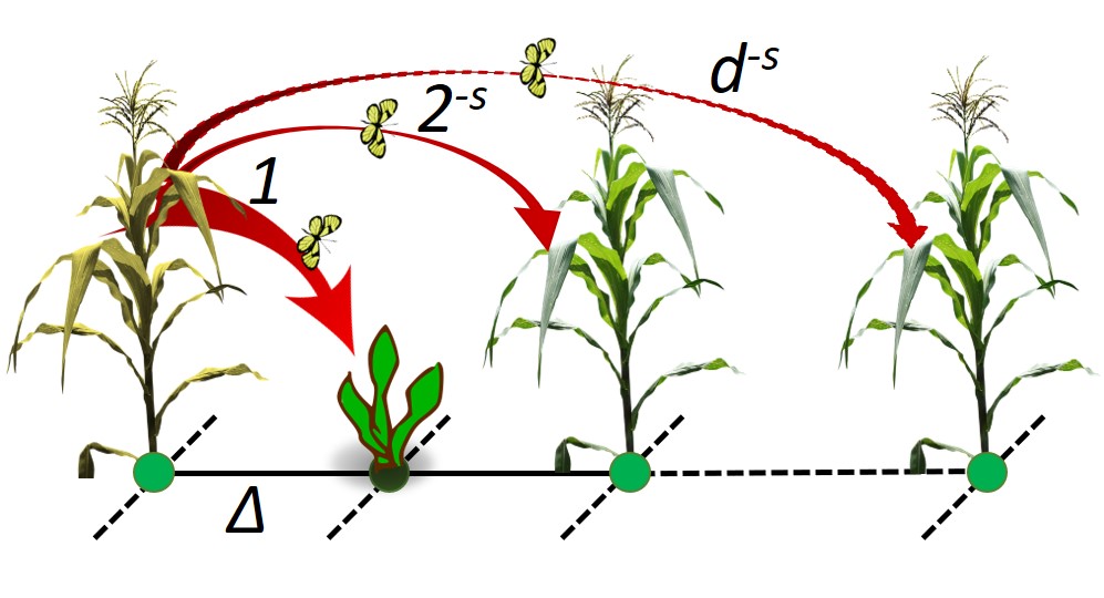
Figure 2.1: Inter-plants movements of an aphid in an agricultural plot with intercropping (see Supplementary Note 1). The hop of an aphid from an infected plant to a susceptible one separated by $d$ steps is given by $d^{-s}$ (see Supplementary Note 1).

The $d$-path adjacency matrices $A_{d}$ used in the current formulation are generalizations of the concept of adjacency matrix. In the Supplementary Note 2 we give a formal definition of them and an example (see also [62, 63, 64]). We will always consider a connected network here. Let $d_{ij}=d$ be the shortest-path distance between the nodes $i$ and $j$ in a network $G$. Then, the $d$-path adjacency matrix is defined by

$$A_{d}\left(i,j\right)=\left\{\begin{array}[]{cc}1&\textnormal{if }d_{ij}=d\\ 0&\textnormal{otherwise}.\end{array}\right.$$ (2.8)

We consider any $1\leq d\leq d_{max}$, where $d=1$ provides the “classical” adjacency matrix and where $d_{max}$ is the diameter of the network. Then, we combine all the $d$-path adjacency matrices by using a transformation, such that

$$\tilde{A}=A_{1}+2^{-s}A_{2}+\cdots+d_{max}^{-s}A_{d_{max}},$$ (2.9)

where $s$ is an empirical parameter controlling the insect mobility. The transformation in Eq. (2.9) is denoted as Mellin $d$-path transformation. In this case, the entries of $\tilde{A}$ are defined as follow:

$$\widetilde{A}\left(i,j\right)=\left\{\begin{array}[]{cc}d_{ij}^{-s}&\textnormal{if }i\neq j\\ 0&\textnormal{if }i=j.\end{array}\right.$$ (2.10)

Notice that the transformed adjacency matrix $\tilde{A}$ is symmetric in the case of undirected networks. Then, when the aphid has very poor mobility $s\rightarrow\infty$, all the entries of $\tilde{A}$, except those equal to one, become zeroes, which indicates that the aphid can only perform hops to nearest neighbors. On the other hand, when the aphid has a very large mobility $s\rightarrow 0$, every entry of $\tilde{A}$ becomes one, which means that the aphid can hop from one plant to another with equal probability independently of their separation in the field.

2.3 Markovian formulation of the epidemiological model.

Following the framework introduced in [69], we formulate a Markovian dynamics that, in principle, is valid for any epidemic prevalence. For that reason, hereafter, we restrict ourselves to this Markovian approach. Let $p_{i}(t)$ be the probability that a node $i$ is infected at time $t$. Then, in the SIR model, the Markovian equations reads as follows:

$$p_{i}(t+1) = p_{i}(t)(1-\mu)+(1-p_{i}(t)-\varrho_{i}(t))q_{i}(t-\tau)\;,$$ (2.11)

$$\varrho_{i}(t+1) = \varrho_{i}(t)+\mu p_{i}(t)\;,$$ (2.12)

where $\varrho_{i}(t)$ is the probability that node $i$ is removed at time $t$. Note that the term $1-p_{i}(t)-\varrho_{i}(t)$ is just $s_{i}(t)$, the probability that a node $i$ is susceptible at time $t$. The expression for the infection probability $q_{i}(t-\tau)$ is [66]

$$q_{i}(t-\tau)=1-\prod_{j=1}^{N}\left[1-\beta\tilde{A}_{ij}p_{j}(t-\tau)\right],$$ (2.13)

which represents the probability that, when node $i$ is healthy at time $t$, it becomes infected at time $t+1$. The expression $q_{i}$ is calculated as $1$ minus the probability that the node $i$ is not infected by any infectious contact. This last probability is the product over all the possible contacts of node $i$, considering that a node $j$ transmits the disease to $i$ with probability $\beta\tilde{A}_{ij}p_{j}$, after the delay time $\tau$. Note that if node $j$ is not connected to $i$ (i.e., if $d_{ij}>1$ and $s\rightarrow\infty$), $\tilde{A}_{ij}=0$, then the corresponding term in the product is equal to $1$, since $j$ cannot infect $i$ regardless of its state, $p_{j}(t-\tau)$.

We should notice that this Markovian formulation holds for any disease incidence, while Eqs. (2.5) and (2.6) are only valid when the disease prevalence is small. To explain this, take Eq. (2.13) for $q_{i}(t-\tau)$ and consider that the prevalence is small, $p_{i}\ll 1$ $\forall i$, and for this reason let us denote $p_{i}=x_{i}$. Then, the product in (2.13) transforms into: $1-\sum_{j=1}^{N}\beta\tilde{A}_{ij}x_{j}$. the new expression for $q_{i}(t)$ in Eq. (2.11), and passing from discrete to continuous time, we recover a similar expression to that in Eq. (2.6) for the evolution of the infected state of node $i$. For more details the reader is referred to [70].

The rate of propagation of the aphid-borne viral infection across an agricultural field is defined here as

$$v=\dfrac{\textnormal{Number of susceptible plants that become removed at equilibrium}}{\mathrm{\textrm{time to reach equilibrium}}}.$$ (2.14)

Finally, for the sake of simplicity, in this work we suppose that the secondary crop of the intercropped systems is not susceptible to the disease and, consequently, its plants can not become infected (i.e. $p_{i}=0$ for every plant $i$ that belongs to the secondary crop). However, note that the presence of a secondary crop may modify the interactions between the plants of the main cultivar (i.e. $d_{ij}$ and $\tilde{A}_{ij}$) and, consequently, their respective probabilities $q_{i}(t-\tau)$. In the next section we define the intercropping arrangements used in this work. Besides, the secondary crop can be used to implement “trap crops”, which may alter mobility of an aphid, i.e. $\tilde{A}_{ij}$ (see subsection 2.4.3).

2.4 Computational arrangements

2.4.1 Intercropping arrangements.

The intercropped systems considered here and shown in Fig. 2.2 are: the strip intercropping in which strips of the main cultivar are inserted between strips of the secondary crop; row intercropping in which rows of the main and secondary crops are alternated one-by-one; column intercropping, the same as before but by columns instead of by rows; chessboard intercropping in which a plant of the main crop is inserted in the rows and columns between every two susceptible plants; patches intercropping in which squared patches of the main crop are alternated with squared patches (of the same size) of the secondary crop; random intercropping in which plants of the secondary crop are randomly inserted among those of the main crop. The first two intercropping arrangements—strips [48, 71] and rows [72, 73, 74]—are frequently used in experimental designs and field applications. It is important to remark that in all cases we have considered exactly the same amount of plants of the main crop such that the results obtained here are not due to size effects.

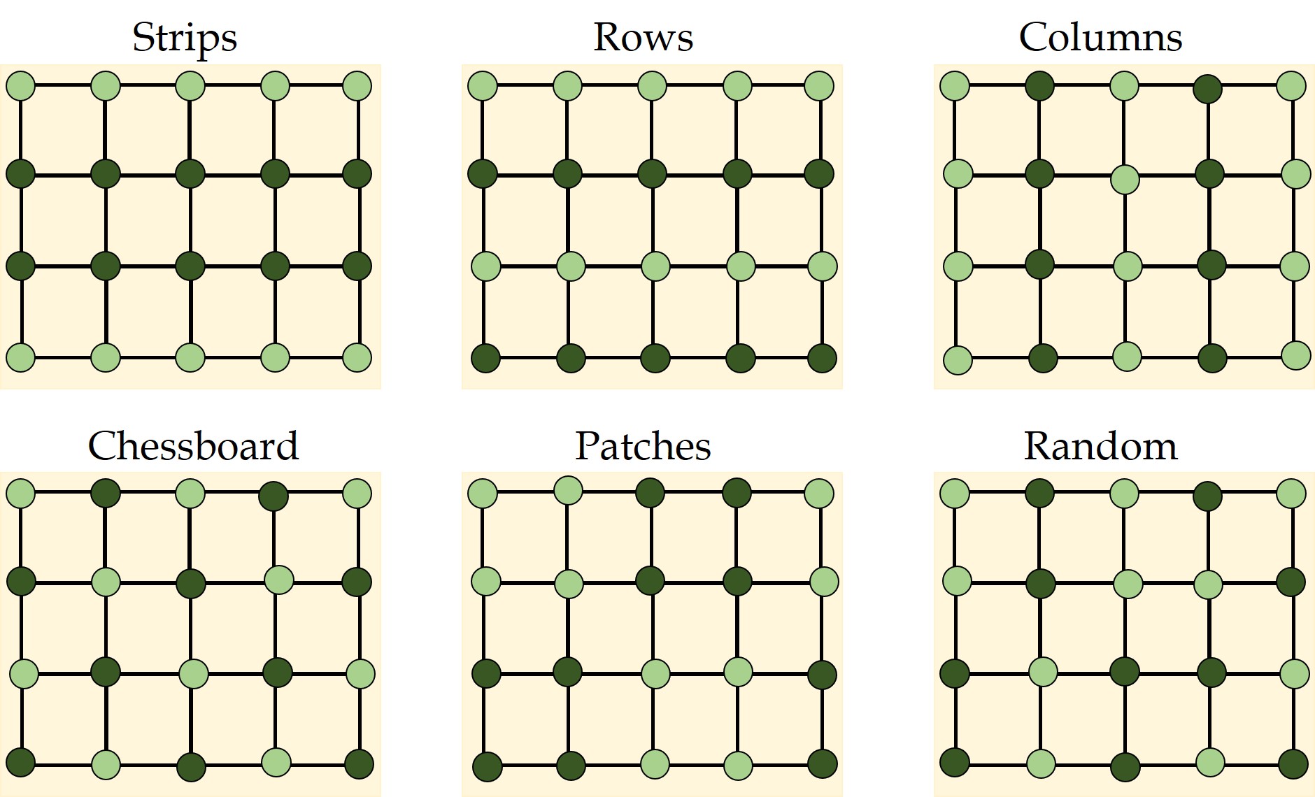
Figure 2.2: Intercrop arrangements. Different organizations of intercrops between two species studied in this work with $r=\varDelta$ (see Networks construction). Light green nodes represent the main crop and the dark green nodes represent the secondary crop, which is considered to be not susceptible to the disease spreading on the field. In the case of trap crop strategies the dark green nodes represent the plants with semiochemical activity to trap the pest to be controlled. The square lattices connecting the nodes correspond to the interconnection networks considered here.

2.4.2 Networks construction.

Our arrangements consist of rectangular plots of lengths $x=a$ and $y=a^{-1}.$ These plots guarantee that all simulations are carried out on fields of equal area. The rectangular plots have been shown–both theoretically and experimentally–to delay more the propagation of epidemics than square plots with the same area and density of plants [75]. We consider the distribution of a major crop intercropped with a secondary crop, which may or may not be a trap crop. In the intercropped field we maintain a separation between plants equal to $\varDelta$ (see Fig. 2.3). In this case the plant-to-plant connectivity, based on their separation, is represented by a squared partition of the plot. We simply normalize all the distances by dividing them by $\varDelta$. Then, two plants which are nearest neighbors are one step apart, a second nearest neighbor is two steps apart and so forth. In general, every plot consists of 20 rows and 50 columns. There is a plant at every intersection for a total of 1000 plants. As we have a unit rectangle with $a=1.6059$, the value of $\varDelta$ is 0.033, and we use a connection radius $r=\Delta,$ such that the plants are adjacent (connected in the network) only to those immediately to the left, right, up and down. In the case of the intercropped systems we always replaced 500 plants of the main crop by the same quantity of plants of the secondary crop. In the Supplementary Note 3 we analyze the case in which the separation between rows and columns in the plot are smaller than $\varDelta$, which is equivalent to consider the radius of primary movement of the aphid equal to $r=\sqrt{2}\Delta$.

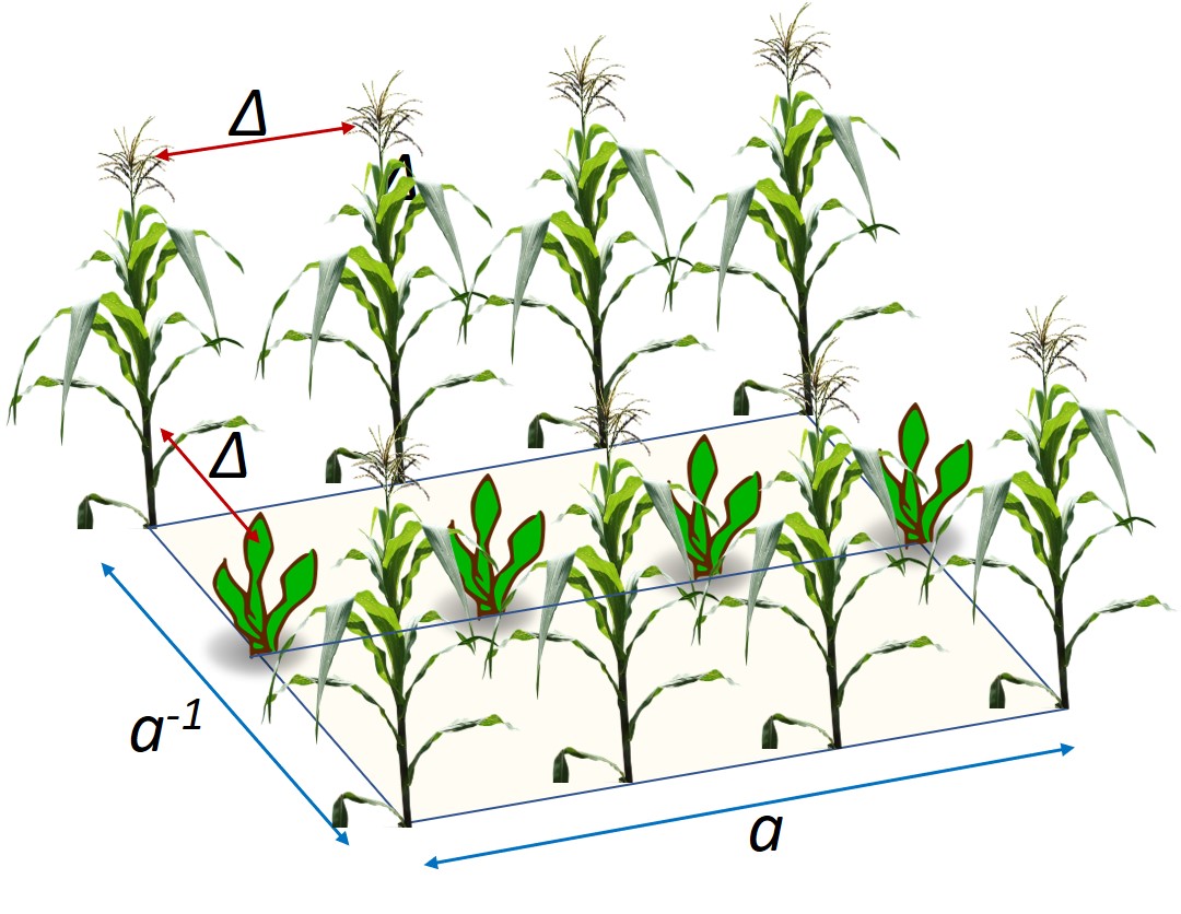
Figure 2.3: Schematic representation of the intercropping of two species in a rectangular plot of unit area and largest edge length $a$. The separation between plants is given by $\varDelta$.

2.4.3 Implementation of the “trap crops”.

Although trap crops can be formed either by “push” crops or by the combination of “push-pull” crops [44, 45, 46, 47], here for the modeling purpose we combine all the trap crop effects into a single one. Basically we consider that trap crop diminishes or completely avoids the propagation of a pest in a path beyond the place in which the trap is located. Consequently, if there are more than one trap in the path between two susceptible plants we only consider the effect of one of them. An additive or multiplicative effect of the traps can be easily implemented using the current mathematical framework (see further), but it is not done here for the sake of simplicity. In this case the secondary crop is located between the paths connecting the infected and the susceptible plants. Mathematically, let us consider two plants $i_{1}$ and $i_{d+1}$, and the shortest-path $i_{1}$, $i_{2}$, $\cdots$, $i_{d}$, $i_{d+1}$ of length $d$ between them. To model trap crops, we modify the strength of the long-range mobility of the aphid between $i_{1}$ and $i_{d+1}$ as follows:

$$\left(\tilde{\mathbf{A}}\right)_{i_{1},i_{d+1}}=\left\{\begin{array}[]{r}d^{-\gamma s}\\ d^{-s}\end{array}\right.\begin{array}[]{l}\textnormal{if there is at least one trap crop between $i_{i}$ and $i_{d+1}$}\\ \textnormal{otherwise}\end{array},$$ (2.15)

where $\gamma\geq 1$ is the trap strength. When $\gamma=1$, there is no trap crop as we recover the original equation for the epidemic dynamics with long-range movements. On the other hand, when $1<\gamma<\infty$, movement of the aphid is reduced beyond the point in which the trap is located. For instance, when the trap crop is very effective, i.e., $\gamma\rightarrow\infty$, the movement of the aphid from $i_{1}$ to $i_{d+1}$ is completely interrupted, which means that the trap is perfect. In the Fig. 2.4(b) we illustrate the effects of a secondary crop in which we obtained the probability $q_{i}$ that the plants in the right part are infected once the three plants on the left side are infected by the pest. To do so, we suppose that $p_{i}=0$ for $i$ spanning over the secondary crop and the plants of the main cultivar that are in the right side of each arrangement, and $p_{i}=1$ otherwise. According to Fig. 2.4, the shortest path distance between the infected and the susceptible plants is always $d=2$, and there is a secondary crop plant between them. Under those conditions, Eq. (2.13) reduces to $q_{i}=1-\left(1-\beta 2^{-s\gamma}\right)^{3}$ for each plant in the right side. Supposing $\tau=0$ (no delay), $s=2.5$ (aphid with large mobility) and $\beta=0.5$, when $\gamma=1$ (no trap), the infectability of the susceptible plants is 24.2%, which represents the effects of an intercropped secondary species. However, when the strength of the trap is $\gamma=2$, the probability that the susceptible plants are infected drops to less than 5%. This probability is reduced to zero as $\gamma$ is subsequently increased.

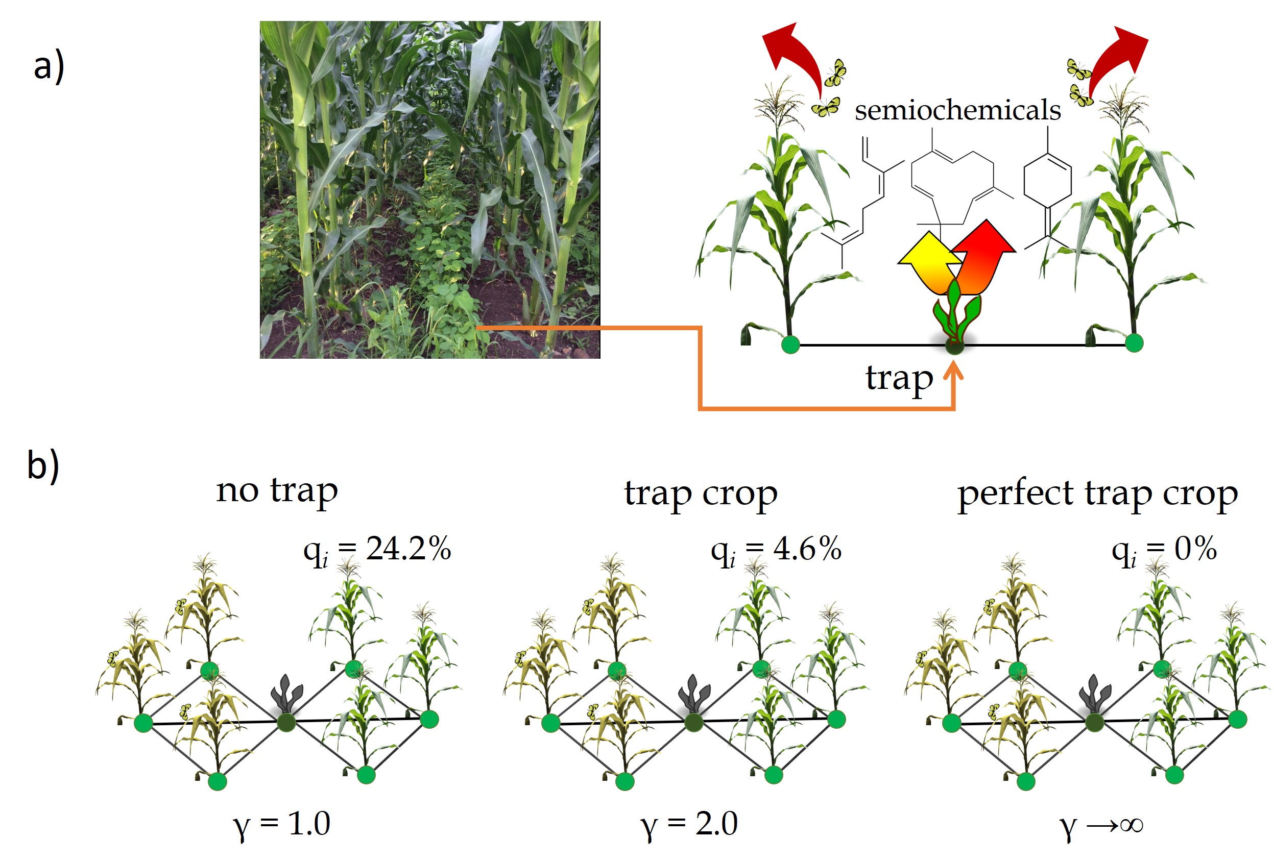
Figure 2.4: (a) Intercropping with ’push’ (or ’push-pull’) strategies where semiochemicals [57, 65] are released from trap crops (the photograph is courtesy of Rachel Monger (Immanuel International)). (b) Effects of the strength of the trap crop $\gamma$ (dark plants) on the probability of plants $i$ to get infected $q_{i}$ (see text for explanations) once the plants on the left of the Fig. are infected.

2.4.4 Simulations.

Using the Markovian formalism, i.e. Eqs. (2.11)-(2.13), we perform 100 random realizations for each field arrangement, secondary crop (with or without trap) and aphid mobility (fast and slow). In each independent realization, the propagation is initialized by infecting randomly a single susceptible plant on the border of the field. Following [66], we set here $\mu=0.5$, since we are not trying to characterize any particular disease. For $\mu=1$, for instance, the recovery is too fast to see the spatial propagation and, conversely, in the case $\mu=0$ the dynamics would be an SI dynamics. We decided to lie between these two limiting cases.

For the dynamics of the disease we calculate the total amount of Markovian time $t^{*}$ in which the probability of being susceptible is larger than the probability of being removed (i.e, $1-\varrho_{i}-p_{i}>\varrho_{i}$), for each plant of the main cultivar. To estimate the epidemic thresholds for a given value of $\gamma$, we calculate the average stationary fraction of removed plants (over 100 independent realizations), $R(\beta,\mu)$, for 50 logarithmically spaced values of $\beta$, between 0.02 and 1.0, when $\mu=0.5$, where $R(\beta,\mu)=\left(1/N_{i}\right)\lim\,_{t\rightarrow\infty}\sum_{i}\varrho_{i}(t)$, $i$ spans over the plants of the main cultivar and $N_{i}$ is the total amount of plants of that crop. Then, using a linear interpolation, we find the epidemic threshold $\tau^{E}$ in each field. We recall that the epidemic threshold is the smallest value of $\beta/\mu$ for each arrangement that satisfies the condition that $R(\beta,\mu)>0$. Visualization of results in the form of rain clouds were performed using Matlab^® codes available from Allen et al. [76]

3 Results and discussion

3.1 Influence of time-delay

According to the results previously reported by Tchuenche and Nwagwo [52], the effects of the time delay $\tau$ are mainly observed at the initial times of the propagation dynamics and are focused on the population of susceptible plants. For relatively large time the evolution of the SIR dynamics with and without time delay are almost indistinguishable (see Fig. 2 in [52]). For instance, in Fig. 3.1 we can observe that the results without time delay, i.e., $\tau=0$ are qualitatively similar to those for $\tau=1$, with almost the same epidemic threshold and very similar shape of the propagation curves. We explore here the effects of $\tau$ on the epidemic dynamics when the vector mobility is incorporated into the model. Using the Markovian formulation described previously in Eqs. (2.11)-(2.13), we obtained the evolution of the infected population of plants in crop field consisting of a square lattice as described before for two different values of the aphid mobility $s$ in the Mellin transformed Markovian SIR equations. The results are illustrated in Fig. 3.1 were we have used $\beta=0.5$, $\mu=0.5$, $r=\varDelta$ and $s=2.5$ (a) and $s=1.0$ (b). It can be seen that the inclusion of a time delay in the model makes that the peak in the number of infected plants is displaced to longer times. For large aphid mobility ($s=1.0$) it is observed that the shapes of the peaks of infection are very similar to each other for different values of the time delay $0\leq\tau\leq 10$. When the mobility of the aphids is relatively low ($s=2.5$) the rate of propagation of the infection changes significantly for different values of $\tau$, particularly for very large time delays. For instance, the values of the rate of propagation for a given time-delay, $v\left(\tau\right)$, obtained from Eq. (2.14), are as follow: $v\left(0\right)=32.25$, $v\left(1\right)=26.32$, $v\left(2\right)=22.22$, $v\left(3\right)=18.87$, $v\left(4\right)=16.67$, $v\left(5\right)=14.70$, $v\left(10\right)=9.17$. However, for the case of large aphid mobility these rates of propagation are not changed significantly with the time delay: $v\left(0\right)=43.48$, $v\left(1\right)=40.00$, $v\left(2\right)=38.46$, $v\left(3\right)=35.71$, $v\left(4\right)=34.48$, $v\left(5\right)=33.33$, $v\left(10\right)=27.78$. That is, for relatively low time delays the results in the disease propagation on plants are very similar to those without time-delays. Also, when the the aphid mobility is relatively large, the time delay does not affect significantly the propagation rate of the disease.

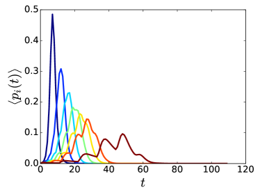
(a)

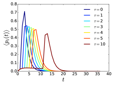
(b)

Figure 3.1: Evolution of the number of infected plants in a square plot with the variation of the time delays $\tau$. The modeling is performed with $\beta=0.5$, $\mu=0.5$, $r=\varDelta$ and $s=2.5$ (a) and $s=1.0$ (b).

As a consequence of the previous analysis and for the sake of keeping our model as simple as possible we are not considering explicitly the time delay in the further calculations in this work. The biological justification for this simplification is as follows. The interaction of the virus and aphid is controlled by the following phases (see Chapter 15 of [19]): (i) acquisition, where the aphid takes up virions from an infected plant, (ii) retention, where the aphid carries the virions at specific sites, (iii) latency, which refers to the inability of an aphid to inoculate immediately a virus following acquisition, and (iv) inoculation, which is the release of retained virions into the tissues of a susceptible plant. There are three types of transmission of a virus to a plant (see Chapter 15 of [19]). In the non-persistent (NP) transmission, the acquisition and inoculation are very fast and requires only a very brief stylet penetration, which delays less than one minute. In this case there is no latency period and the whole cycle of transmission can be completed within a few minutes. In the semi-persistent (SP) transmission, the acquisition and inoculation requires periods of about 15 minutes. In this case there is no latency periods either and the aphids retain the ability to inoculate for periods of up to 2 days following acquisition. Finally, in the persistent (P) transmission the virus acquisition requires period between hours to days, there is a latency period and the retention is for days to weeks. From the about 270 viruses transmitted by aphids more than 200 are transmitted by NP transmission (see Chapter 15 of [19]). The results to be considered here using a SIR model without time delays is then equivalent to model the aphid-borne transmission of viruses to plants using either NP or SP transmission.

3.2 Impact of intercrop arrangements on virus propagation.

In Fig. 3.2 we illustrate the results of the simulations of the propagation of an aphid-borne virus in the 6 intercropped fields without traps $(\gamma=1.0$) studied here as well as in the monocrop. In Fig. 3.2 (a) we show the results for an aphid with relatively low mobility ($s=4.0$) and in Fig. 3.2 (b) we give the same for a relatively high mobility aphid ($s=2.5$). To compare the dynamics of the different arrangements, firstly, we analyze their respective results before they reach equilibrium ($t=10$). In the case in which $s=4.0$ it is clear that the disease is propagated in a relatively slow fashion and for $t=10$ only 18.3% of plants are removed in the monocrop. As can be seen in this figure all intercrop arrangements produce significant decrease in the number of removed plants. The smallest decay in the number of removed plants is observed for the patches configuration in which the percentage of removed plants is 10.1%, followed by the strips configuration with 6.6%. On the other hand, the most efficient arrangement is the chessboard one, which reduces the number of removed plants practically to zero (only 0.3% of removed plants).

In Fig. 3.2 (b) we illustrate the results for the case in which the pest has a relatively large mobility. Here the picture observed is significantly different from the one in the previous case. First, the level of plants removed in the monocrop is 95.1%, indicating an almost complete destruction of the crop in a relatively short time ($t=10$) when the pest is highly mobile. The range of amelioration of the infection across the fields is here very wide, ranging from the 10% of decrease in removed plants observed for the patches arrangement (85.5% of removed plants) up to about 80% of decrease obtained with the chessboard arrangement (16.3% of removed plants). Notice that the frequently used intercrop arrangement of strips produces, together with that of patches, the smallest improvement in the number of removed plants. Thus, although the results are quantitatively very different for the cases of low and high mobility of the aphid, they are qualitatively similar in identifying the worse arrangements (patches and strips) as well as the best one (chessboard). In both cases the order of effectivity in reducing the impact of an aphid-borne virus propagation is: chessboard > columns > random > rows > strips > patches.

In Fig. 3.2 (c) and (d) we illustrate a snapshot of the aphid-borne propagation of a virus across the different intercropping systems with $s=4.0$ and $s=2.5$, respectively. In order to compare all the different arrangements we always start the epidemic by infecting the same node, i.e., the one at the bottom-left corner of the field. The colors in the plots represent the time $t^{*}$ in which the plant remains susceptible without becoming removed by the vector-borne virus disease. That is, a low value of this time indicates that the plant is removed relatively soon by the virus disease. In order to interpret quantitatively the results in these plots we use the rate $v$ of propagation of the aphid-borne virus previously defined in Eq. (2.14). It can be seen that in the monocrop the epidemic is propagated in a wave-like way, typical of diffusion processes. The values of $v$ in the monocrop are 23.26 ($s=4.0$) and 32.26 ($s=2.5$). That is, when the aphid has relatively low mobility there is an average infection of 23.26 plants per unit time. This rate is increased to 32.26 plants when the pest mobility is increased, due to the fact that the aphids can now hop to wider regions of the plots. Reminiscences of the wave-like kind of propagation of the vector-borne virus are observed in all the intercrop arrangements studied. In the intercropped systems (without trap crops, $\gamma=1.0$) the propagation rates of the virus are: for $s=4.0$, chessboard (0.03) < random (5.46) < columns (7.35) = rows (7.35) < strips (10.0) < patches (11.36); for $s=2.5$, chessboard (9.62) < random (12.19) < columns (13.16) = rows (13.16) < strips (14.70) < patches (15.62). In closing, the chessboard arrangement is significantly better in reducing the propagation of aphid-borne viruses in agricultural fields than the rest of the arrangements when there are no trap crops in the intercrop. The random arrangement also performs very well in terms of both the number of plants removed by the infection and the rate of propagation of the epidemic.

Finally, it is worth recalling that the prior results depend on the radius for primary dispersal of the aphid. See Supplementary Note 3 for the case when the separation between rows and columns is smaller than here and the pest can hop not only across the rows and columns, but also diagonally between rows, i.e., when the radius for primary dispersal of the aphid is $r=\sqrt{2}\varDelta$ instead of $r=\varDelta.$ When the pest mobility is relatively low ($s=4.0$), the best arrangements are the rows and columns intercrops with about 10% of affected plants vs. 78% affected in the monocrop for $t=10$. However, when the pest has high mobility ($s=2.5$), none of the intercropping systems is able to stop the propagation of the pest across the field, with percentages of affected plants similar to that in the monocrop (98.6%). An obvious measure to mitigate this problem is to increase the separation of the rows and columns in the crop field, or even–as shown in the experiments by Khan et al. [28]–to increase the separation between rows keeping a smaller separation between columns.

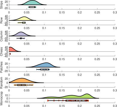
(a)

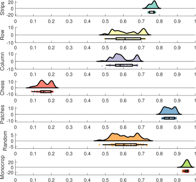
(b)

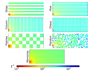
(c)

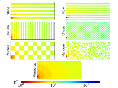
(d)

Figure 3.2: Aphid-borne virus propagation on intercropped fields without traps. Results of the simulations for a SIR epidemics at $t=10$ with $r=\varDelta,$ $\beta=0.5,$ $\mu=0.5$ for different intercropping strategies without trap crops, i.e., the strength of the trap crop is $\gamma=1.0$. Raincloud plots of the proportion of dead plants for a viral infection propagated by aphids: (a) Aphid with reduced mobility ($s=4.0)$ and (b) with larger mobility ($s=2.5$). The clouds show the kernel distribution of the proportion of dead plants for different realizations of the epidemics. Below, the raw data is plotted (the rain) together with their corresponding box and whisker plots. Illustration of the evolution of infection across fields with different intercropping systems: (c) Aphid with reduced mobility ($s=4.0)$ and (d) with larger mobility ($s=2.5$). In both panels the time $t^{*}$ is given in a color scale (see text), and the propagation is initialized by infecting the plant on the bottom-left corner of the plot.

3.3 Impact of intercrops with trap crop on aphid-borne virus propagation.

We now move to the analysis of the intercrop systems with trap crops. To have an idea of the many systems in which the current results can be applied the reader is referred to the Tables 1 and 2 in Hokkanen’s paper [44], where many examples of one main crop intercropped with a trap crop are given. We consider here the existence of trap crops which are not perfect, i.e., they allow certain propagation of the aphid-borne viral infection (see Supplementary Note 4 for results with a perfect trap). Thus, we use $\gamma=2.0$ and analyze the cases of relatively low ($s=4.0$) and relatively large ($s=2.5$) aphid mobility. In Fig. 3.3 we illustrate the results of our simulations for these systems using the different arrangements studied here. As can be seen for the case of relatively low mobility ($s=4.0$) there are significant reduction in the percentages of removed plants for all intercrop systems. The percentages of removed plants for each intercrop are: chessboard (0.2%), columns (1.4%), random (1.5%), rows (1.8%), strips (3.4%) and patches (4.7%). We remind the reader that the percentage of removed plants in the monocrop is 18.1%. When the pest has a relatively large mobility ($s=2.5$), 95.1% of plants are removed in the monocrop, while in each of the intercrops they are: chessboard (0.2%), random (2.8%), columns (4.4%), rows (6.3%), patches (9.1%), and strips (17.4%). Notice that here there are some important changes in the order of the arrangements in terms of their effectivity in reducing the propagation of the infection. When the aphid is of high mobility the best arrangements are the chessboard and the random one. The worse arrangement, and the only one having more than 10% of removed plants, is the strip one. Also notice that the percentage of removed plants in the chessboard arrangement is exactly the same for $s=2.5$ and $s=4.0$, indicating a high stability in the efficiency of this arrangement. It is important to remark one more time that these reductions in the number of removed plants are the consequence of the different topological patterns emerging from the intercrop arrangements. That is, these differences are not a dilution effect due to the fact that the number of susceptible and immune plants are kept the same in every arrangement.

We now analyze the rate of propagation of the aphid-borne virus across the agricultural fields intercropped with a trap crop (see Fig. 3.3 (c) and (d)). The rate of propagation of the virus follow a different order as for the case of intercrops without traps ($\gamma=1.0$). That is, for $s=4.0$, we find: chessboard (0.05) < random (1.67) < columns (4.59) < rows (4.67) < strips (7.04) < patches (7.94). For $s=2.5$, chessboard (0.04) < random (4.18) < columns (7.58) < rows (8.06) < strips (10.87) < patches (11.63). Here again there is a significantly high improvement, in terms of diminishing the impact and the rate of propagation of a virus across an agricultural field, when the chessboard arrangement is used. See Supplementary Note 3 for the case when the separation between rows and columns is smaller than here, i.e., when the radius for primary dispersal of the aphid is $r=\sqrt{2}\varDelta$ instead of $r=\varDelta.$ These results agree with those previously reported using a different stochastic simulation model [67].

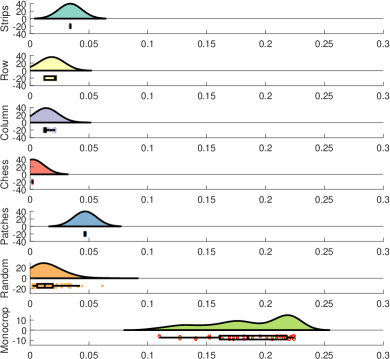
(a)

(b)

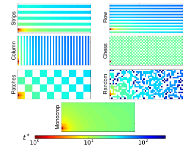
(c)

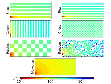
(d)

Figure 3.3: Aphid-borne virus propagation on intercropped fields with trap crops. Results of the simulations for a SIR epidemics at $t=10$ with $r=\varDelta,$ $\beta=0.5,$ $\mu=0.5$ for different intercropping strategies with trap crops of strength $\gamma=2.0$. Raincloud plots of the proportion of dead plants for a viral infection propagated by aphids: (a) Aphid with reduced mobility ($s=4.0)$ and (b) with larger mobility ($s=2.5$). The clouds show the kernel distribution of the proportion of dead plants for different realizations of the epidemics. Below, the raw data is plotted (the rain) together with their corresponding box and whisker plots. Illustration of the evolution of infection across fields with different intercropping systems: (c) Aphid with reduced mobility ($s=4.0)$ and (d) with larger mobility ($s=2.5$). In both panels the time $t^{*}$ is given in a color scale (see text), and the propagation is initialized by infecting the plant on the bottom-left corner of the plot.

3.4 Epidemic thresholds.

Finally we study the ratio $\beta/\mu$, which drives the spreading of the disease. Depending on the infectious power of the aphid-borne virus there are two possible distinguishable phases for a given strength of the trap crop, $\gamma$, and of the pest mobility, $s$. The first one is an absorbing phase where the spreading of the virus is not efficient enough to reach a large fraction of the system and the propagation is absorbed, meaning that it does not progress across the field. The second phase is an active one, where the propagation of the virus reaches a macroscopic fraction of the agricultural field. The transition from the absorbing to the active phase strictly resembles a non-equilibrium second order phase transition in statistical physics [68]. The critical value of this transition $\left(\frac{\beta}{\mu}\right)_{c}=\tau^{\,E}$ is defined as the epidemic threshold. This term is also know as the basic reproduction number and it represents a threshold in the sense that below this point the propagation of the infection dies out and over it the propagation becomes an epidemic. We have then investigated the epidemic threshold $\tau^{\,E}$ for the monocrop and the six intercrop arrangements without ($\gamma=1.0)$ and with a trap crop ($\gamma=2.0)$. We also considered, as before, two kinds of aphid, one with relatively low mobility ($s=4.0)$ and the other with higher mobility ($s=2.5)$. In Fig. 3.4 we resume the results. Let us first consider the intercropped fields without trap crops ($\gamma=1.0$). Then, when the pest has low mobility the epidemic threshold of the chessboard arrangement is more than 10 times higher than that of the monocrop. Notice that we have normalized all the bar plots in the insets of Fig. 3.4 by dividing the epidemic thresholds by that of the monocrop. Indeed, we have proved in the Supplementary Note 5 that the chessboard arrangement can reach an infinitely large epidemic threshold if $s$ is bounded and the trap crop has a very high strength. The rest of the arrangements have epidemic thresholds which are about twice that of the monocrop. When the aphid mobility increases, the epidemic thresholds logically drop, due to the fact that it is easier for the pest to trigger the propagation of a virus across the field. In this case the chessboard arrangement triplicates the epidemic threshold of the monocrop, while the rest of the arrangements have values of about 1.5 times larger than the one of the monocrop. When we incorporate trap crops ($\gamma=2.0$) in the intercrop arrangements the changes in the epidemic threshold results very dramatic for the case of the chessboard arrangement. In this case, with low and high mobility, the epidemic thresholds are about 40 and 32 times higher than that of the monocrop. For the rest of the intercropped systems the threshold increases by factors between 2 and 5. It is interesting that for the rest of the intercrop systems the ordering of the epidemic thresholds vary from one scenario to another. For instance, without trap crop and low mobility of the pest, the random arrangement is the second best, followed by the rows arrangement. However, if the aphid has larger mobility the column arrangement is the second best followed by the rows one. When there are trap crops and low mobility of the pest the rows arrangement is the second best followed by the columns one. If the mobility of the pest is higher then the column is the second best followed by the strips one. It is possible that the empirical observation that the rows and strips arrangement delay the propagation of an aphid-borne virus in a crop field has made that these two arrangements have been the most widely used ones. However, in terms of (i) percentage of plants removed by the infection, (ii) rate of the propagation of the aphid-borne virus across the field, and (iii) epidemic threshold, the chessboard arrangement introduced here is by far the most efficient intercrop arrangement without and with trap crops. In this respect our model agrees with previous results showing that the finer grained mixing of susceptible and resistant species impedes the propagation of diseases on plants [77, 78, 79]. However, as we have also shown in this work, when the radii of aphid movement increases, then other intercropping arrangements such as the column, rows and random, are very efficient to stop the propagation of diseases across a field.

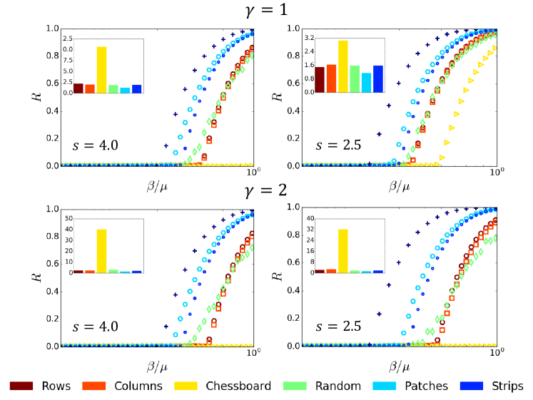
Figure 3.4: Epidemic thresholds for the propagation of aphid-borne viruses on intercropped fields. Effects of the strength of the trap crop $\gamma$ and of the pest mobility $s$ on the number of removed (dead) plants during the propagation of an aphid-borne virus infection across intercropped fields with $r=\varDelta$. The case for $\gamma=1$ corresponds to no trap crop. The symbols used for each intercrop are: strips (small circles), rows (large circles), columns (squares), chessboard (triangles), patches (hexagons), random (diamonds), and monocrop (crosses). In the insets we illustrate the normalized epidemic thresholds for each of the intercrop arrangements. The normalization is obtained by dividing every epidemic threshold by that of the monocrop in the corresponding system. The color code for the insets is given at the bottom of the figure.

Conclusion

Here, we demonstrate using intensive mathematical modeling, that the efficiency of intercropping arrangements can be improved dramatically in relation to the designs currently in use. We develop a mathematical framework that allows to study the effect of intercropping systems with and without ’trap crops’. Our study shows that improving existing intercrop designs may decrease up to 80% the number of plants affected by aphid-borne viruses, slow down the propagation of such aphid-borne viruses by a 300-fold factor, and delay the triggering of these epidemics on plants by a 40-fold factor respect to a monocrop. Indeed, our analytical and numerical findings show that the chessboard is the best arrangement when the pest can hop only across the rows and columns, but not diagonally between rows.

Supplementary Tables

intercrop system	intercrop system	intercrop system	intercrop system
alfalfa_potato [1]	maize_cowpea	maize_mungbean	sorghum_groundnut
barley_pea	maize_wheat	maize_egusi melon	sorghum_soybean
barley_clover	maize_faba beans	maize_ alfalfa	sorghum_cowpea
barley_medic	maize_soybean	mustard_legume	soybean_sunflower
barley_faba	maize_bean	oat_faba beans	strawberry_broad beans
barley_vetch	maize_bean_squash	oat_common vetch	sweet potato_jugo beans
barley_chickpea	maize_canola	oat sown_vetch	wheat_faba beans
coffee_macuaba [2]	maize_tobacco	okra_pumpkin	wheat_soybean
cowpea_soybean	maize_sugarcane	okra_sweet potato_	wheat_canola
cowpea_cotton	maize_potato	onion_pepper	wheat_chickpea
faba beans_pea	maize_peanut	radish_amarantus	wheat_common vetch
faba_teff	maize_legume	rice_blackgram	wheat_lentils
fennel_dill	maize_okra	sesame_sunflower	wheat_cotton
leek_celery	maize_groundnut	sorghum_legume
lentils_fenu greek	maize_peanut	sorghum_sunflower

Table 1: Illustration of some intercropped systems reported by Brookers et al. [3], Martin-Guay et al. [4] and references therein.

Supplementary Note 1

In formulating the “rationale of the model” we consider that two plants $i$ and $j$ are separated by a geographic (Euclidean) distance equal to $\rho_{ij}$. We consider that the aphid has a radius of primary exploration equal to $r$. That is, the aphid can hop directly from the plant $i$ to any other plant in a radius $r$ from $i$. Then, if two plants are at a distance $\rho_{ij}\leq r$ we consider that they are topologically connected to each other by an edge. The number of edges in the shortest path connecting two plants $i$ and $k$ (not directly connected to each other) is the topological distance $d_{ik}.$ We consider here two different kinds of hopping probabilities. The geographic hopping probability $\pi_{ij}$ depends on the geographic distance between the two plants, e.g., $\pi_{ij}\propto\rho_{ij}^{-s}$. The topological hopping probability depends only on the topological distance separating the two plants, and not on its geographic separation, e.g., $p_{ij}\propto d_{ij}^{-s}$. Then, we have the following rules.

First come first served. Consider an aphid at a plant $i$ which can hop to any of the adjacent plants $j$ (left) or $k$ (right) (see Supplementary Figure 3.5(a)). Let us consider that the geographic distance between the plants are $\rho_{ij}<r$ and $\rho_{ik}<r$, respectively, such that $\rho_{ij}>\rho_{ik}$. Then, according to the geographic distance, the probability of the aphid hopping to plant $k$ is larger than that of hopping to plant $j$, i.e., $\pi_{ij}\propto\rho_{ij}^{-s}$ and $\pi_{ik}\propto\rho_{ik}^{-s}$ assuming a power-law decay with the distance, thus $\pi_{ij}<\pi_{ik}$. However, as the plants $j$ and $k$ are inside the radius of primary movement of the aphid, an aphid hopping from $i$ to the right will find first the plant $k$, exactly the same as an aphid hopping to the left who will find first the plant $j$. Thus, both hopping processes should display the same probabilities, which is accounted for by the topological distance between the pairs of plants. Because $\left(i,j\right)$ are nearest neighbors as well as $\left(i,k\right)$, we have that $d_{ij}=d_{ik}=1$, where $d_{ij}$ is the topological (shortest path) distance. Consequently, $p_{ij}=p_{ik}$. operators

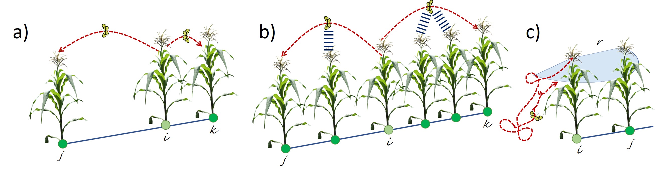
Figure 3.5: (a) Illustration of the “first come first served” hopping process of an aphid between plants. (b) Illustration of the exploratory strategy of aphid based on “a bird in the hands is worth than two in the bush”. (c) Illustration of the plausible returning strategy of an aphid after overpassing its exploratory radius without finding other plants to land in.

A bird in the hand is worth more than two in the bush. Consider an aphid at a plant $i$ which can hop either to plants on its left or on its right (see Supplementary Figure 3.5 (b)). Let us consider that the geographic distances between the plants are $\rho_{ij}$=$\rho_{ik}>r$. Then, according to the geographic distance, the probability of the aphid to hop to plant $k$ is exactly the same as that of hopping to plant $j$, i.e., $\pi_{ij}=\pi_{ik}\propto\rho_{ij}^{-s}$ assuming a power-law decay with the distance. However, an aphid moving from $i$ to the left will find first a plant in its way to $j$. Thus, assuming that such plant is attractive to it, the aphid will explore first that plant on the basis of a minimum effort principle and then the plant $j$. On the other hand, an aphid moving from $i$ to the right will find first a plant that it can explore and in case it decides to continue its movement to the right, the aphid will find yet another plant before arriving at $k$. Thus, it is clear that under the same conditions the probability of arriving at the plant $k$ is smaller than that of arriving at $j$, although they are at exactly the same geographic distances. Assuming the connectivity of the plants given in Supplementary Figure 3.5 (b) we have that $2^{-s}\propto p_{ij}>p_{ik}\propto 3^{-s}$.

Go back before it is too late. Consider an aphid having an exploratory movement at the borderline of a crop field from a node $i$ (see Supplementary Figure 3.5(c)). If the aphid is moving away from the field there is a high probability that it overpass its exploratory radius before finding a new plant. Thus, it is probable that the aphid returns to plant $i$ before finding any new one. As a consequence, the probability that the aphid arrives at a plant distant from $i$ depends more on the topological separation among the plants than on the geographic distance through the “possibly empty” space separating them. That is, we consider here that an aphid navigates a crop field by orienting itself through the plants and not realizing “risky” explorations outside the field.

Supplementary Note 2

More formally, $\tilde{A}$ is a transformed adjacency operator on a graph, which will be defined as follows. Let us consider $\Gamma=(V,E)$ to be an undirected finite or infinite graph with vertices $V$ and edges $E$. We assume that $\Gamma$ is connected and locally finite (i.e. each vertex has only finitely many edges emanating from it). Let $d$ be the shortest path distance metric on $\Gamma$, i.e. $d(v,w)$ is the length of the shortest path from $v$ to $w$. Let $\ell^{2}(V)$ be the Hilbert space of square-summable functions on $V$ with inner product

$$\langle f,g\rangle=\sum_{v\in V}f(v)\overline{g(v)},\qquad f,g\in\ell^{2}(V).$$ (3.1)

In $\ell^{2}(V)$ there is a standard orthonormal basis consisting of the vectors $e_{v}$, $v\in V$, where

$$e_{v}(w)=\begin{cases}1&\text{if $w=v$},\\[2.15277pt] 0&\text{otherwise}.\end{cases}$$ (3.2)

For $d\in\mathbb{N}$ the following operator defined in $\ell^{2}(V)$ is the $d$-path adjacency operator of the graph

$$\bigl{(}A_{d}f\bigr{)}(v)\coloneqq\sum_{w\in V:\,d(v,w)=d}\bigl{(}f(w)\bigr{)},\qquad f\in\ell^{2}(V),v\in V$$ (3.3)

The $d$-path adjacency operator acts over the vectors $e_{v}$ as

$$(A_{d}e_{v})(w)=\begin{cases}1&\text{if $d(v,w)=d$},\\[2.15277pt] 0&\text{otherwise}.\end{cases}$$ (3.4)

These operators are the adjacency analogues of the $d$-path Laplacian operators of the graph [62, 63, 64]. The Mellin (power-law) transformed adjacency operator is then defined by

$$\tilde{A}\coloneqq\sum_{d=1}^{d_{max}}d^{-s}A_{d}.$$ (3.5)

Other transforms are also possible as the Laplace (exponential) one (see for instance [62, 63, 64] for the analogues in the path Laplacians), but we constraint ourselves here to the power-law one.

For instance, if we consider a rectangular lattice like the one illustrated in the Supplementary Figure 3.6 in which we have labeled the nodes using numbers from 1 to 12. The corresponding Mellin transformed $d$-path adjacency matrix for this network is given below for a generic value of the insect mobility $s$:

$\tilde{A}=\left(\begin{array}[]{cccccccccccc}0&1&2^{-s}&3^{-s}&1&2^{-s}&3^{-s}&4^{-s}&2^{-s}&3^{-s}&4^{-s}&5^{-s}\\ &0&1&2^{-s}&2^{-s}&1&2^{-s}&3^{-s}&3^{-s}&2^{-s}&3^{-s}&4^{-s}\\ &&0&1&3^{-s}&2^{-s}&1&2^{-s}&4^{-s}&3^{-s}&2^{-s}&3^{-s}\\ &&&0&4^{-s}&3^{-s}&2^{-s}&1&5^{-s}&4^{-s}&3^{-s}&2^{-s}\\ &&&&0&1&2^{-s}&3^{-s}&1&2^{-s}&3^{-s}&4^{-s}\\ &&&&&0&1&2^{-s}&2^{-s}&1&2^{-s}&3^{-s}\\ &&&&&&0&1&3^{-s}&2^{-s}&1&2^{-s}\\ &&&&&&&0&4^{-s}&3^{-s}&2^{-s}&1\\ &&&&&&&&0&1&2^{-s}&3^{-s}\\ &&&&&&&&&0&1&2^{-s}\\ &&&&&&&&&&0&1\\ &&&&&&&&&&&0\end{array}\right)$

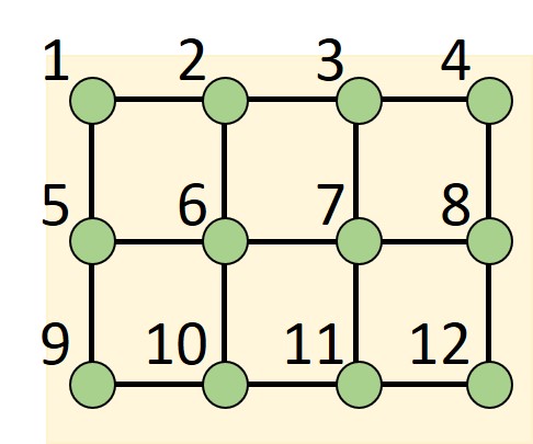
Figure 3.6: Illustration of a rectangular lattice with nodes labeled.

Supplementary Note 3

We consider the situation in which the insect pest has a radius for short-range dispersal–searching, foraging, ranging, etc.–which is larger than the one considered in the main text. The influence of the inter-rows separation was previously considered by Sheoran et al. experimentally [8]. However, their analysis is only from the bio-economical point of view and not from that of pest management. Here we consider $r=\sqrt{2}\varDelta$ instead of $r=\varDelta$, which gives rise to networks like the one illustrated in the Supplementary Figure 3.7. This situation naturally emerges if we consider that the rows and columns of the crop field are too close together, such that the pest can hop not only across the rows and columns, but also diagonally between rows. To notice the difference between this network and the square one produced by $r=\varDelta$ we simply should count the number of steps a pest need to traverse the plot through its diagonal. In the square lattice the number of steps needed is $D=c+r-2$, where $c$ is the number of columns, and $r\leq c$ is the number of rows. However, in the lattice emerging from $r=\sqrt{2}\varDelta$ we have $D=c-1$, which is always smaller that the previous one if $c>1$. This difference is important as it will provide strategies to mitigate the pest damages produced in this kind of arrangements.

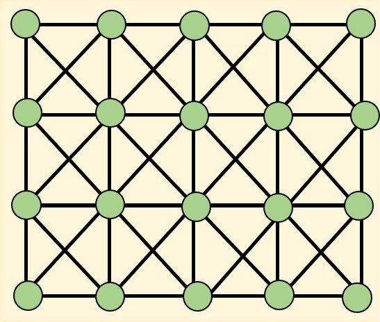
Figure 3.7: Network obtained for a monocrop in which the radius of foraging of the insect pest is $r=\sqrt{2}\varDelta$ instead of $r=\varDelta$.

In the Supplementary Figure 3.8 we give the results for the simulations of a pest propagation in these crop fields when there are no trap crops ($\gamma=1.0$). When the pest mobility is relatively low ($s=4.0$) the best arrangements are the rows and columns intercrops with about 10% of affected plants vs. 78% affected in the monocrop. In this case the chessboard and random intercrops have 30% of affected plants and are the second best, followed by strip (31%), and patches (57%). The rate of propagation $v$ indicates that pests propagating across a monocrop infestates 29.4 plants per unit of time, vs. 9 plants infected in the rows and column arrangements, and 10 plants in the random or 12 in the chessboard. The situation is considerably worsened when the pest has high mobility ($s=2.5$). In this case none of the intercropping systems is able to stop the propagation of the pest across the field with percentages of affected plants ranging 93-98%, not different from that in the monocrop (98.6%). The rates of propagation are reduced to about a half relative to that in the monocrop (37 plants infected per unit time). The reason for this catastrophic result is that a pest with relatively high mobility can infestate very quickly large neighborhoods of a plant due to the possibility that it has of infecting plants in any direction from its current position. An obvious measure to mitigate this problem is to increase the separation of the rows and columns in the crop field, or even–as shown in the experiments by Khan et al. [9]–to increase the separation between rows keeping a smaller separation between columns.

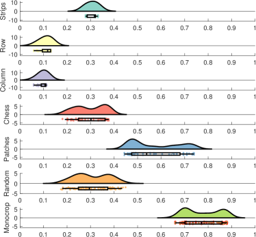
(a)

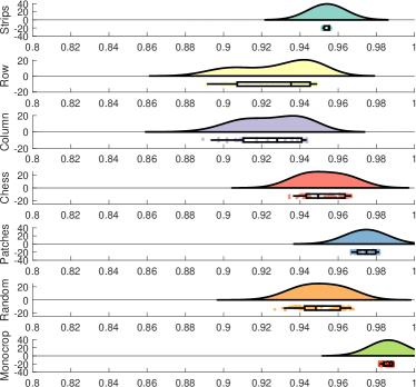
(b)

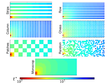
(c)

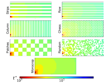
(d)

Figure 3.8: Results of the simulations for a SIR epidemics at $t=10$ with $r=\sqrt{2}\varDelta$, $\beta=0.5,$ $\mu=0.5$ for different intercropping strategies without traps ($\gamma=1.0$). (a) Raincloud plot of the proportion of dead plants for pest with reduced mobility ($s=4.0)$. (b) Raincloud plot of the proportion of dead plants for pest with relatively high mobility ($s=2.5$). The clouds show the kernel distribution of the proportion of dead plants for different realizations of the epidemics. Below, the raw data is plotted (the rain) together with their corresponding box and whisker plots. (c) Evolution of the propagation of a relatively low mobility pest ($s=4.0)$ across the fields. (d) Evolution of the propagation of a relatively high mobility pest ($s=2.5)$ across the fields. In both cases the propagation is initialized by infecting the plant on the bottom-right corner of the plot.

When the trap crops ($\gamma=2.0$) are implemented in the different arrangements the situation resembles more the results reported in the main paper (see Supplementary Figure 3.9). When the pest has low mobility ($s=4.0)$ the percentage of affected plants in the monocrop is 77% while those in the columns and rows intercrops are 1.4% and 1.9%, respectively, followed very closely by the chessboard arrangement with 2.1% of affected plants. When the trap crops are implemented the percentage of plants affected reaches its minimum for the random arrangement (2.1%) followed by columns (4.0%), rows (5.8%), patches (6.2%) and chessboard (6.4%). Only the strips intercrop has higher percentage of affected plants (26.2%). The rates of propagation of the pest follows similar patterns as the one observed for the percentage of affected plants.

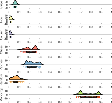
(a)

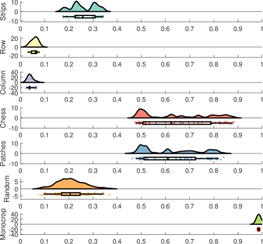
(b)

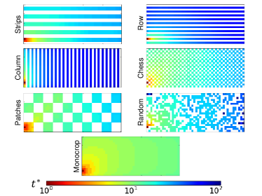
(c)

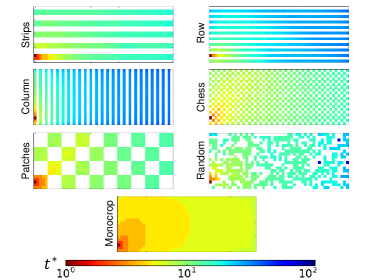
(d)

Figure 3.9: Results of the simulations for a SIR epidemics at $t=10$ with $r=\sqrt{2}\varDelta$, $\beta=0.5,$ $\mu=0.5$ for different intercropping strategies with trap crop of strength $\gamma=2$. (a) Raincloud plot of the proportion of dead plants for pest with reduced mobility ($s=4.0)$. (b) Raincloud plot of the proportion of dead plants for pest with relatively high mobility ($s=2.5$). The clouds show the kernel distribution of the proportion of dead plants for different realizations of the epidemics. Below, the raw data is plotted (the rain) together with their corresponding box and whisker plots. (c) Evolution of the propagation of a relatively low mobility pest ($s=4.0)$ across the fields. (d) Evolution of the propagation of a relatively high mobility pest ($s=2.5)$ across the fields. In both cases the propagation is initialized by infecting the plant on the bottom-right corner of the plot.

The most important conclusion of this Supplementary Note is that the separation between rows and columns in the crop fields should guarantee that the “trivial” dispersal of the pest should be reduced as much as possible. Otherwise, the use of intercropping without trap crops is very inefficient when the pest mobility is relatively high. In any case, the use of trap crops continues to be the most effective approach even in the case when the rows/columns separation is not large enough as to limit the pest “trivial” dispersal.

Supplementary Note 4

We consider intercrop systems with “perfect” trap crops. That is, we use $\gamma\rightarrow\infty$ for the two cases previously analyzed of relatively low ($s=4.0$) and relatively large ($s=2.5$) pest mobility. The result of this scheme is that the pest cannot hop from one susceptible plant to another if in the shortest path connecting them there is at least one trap. In the Supplementary Figure 3.10 we illustrate the results of our simulations for these systems using the different arrangements studied here. As can be seen for the case of relatively low mobility ($s=4.0$) there are significant reduction in the percentages of affected plants for all intercrop systems. The percentages of affected plants for each intercrop are: chessboard (0.2%), columns (1.3%), random (1.5%), rows (1.7%), strips (3.4%) and patches (4.6%). We remind the reader that the percentage of affected plants in the monocrop is 18.1%. When the pest has a relatively large mobility ($s=2.5$) 95.1% of plants are affected in the monocrop, while in each of the intercrops they are: chessboard (0.2%), random (1.8%), columns (2.5%), rows (3.9%), patches (4.8%), and strips (13.6%). Notice that here there are some important changes in the order of the arrangements in terms of their effectivity in reducing the propagation of the pest. When the pest is of high mobility the best arrangements are the chessboard and the random one. The worse arrangement, and the only one having more than 10% of affected plants, is the strip one. Also notice that the percentage of affected plants in the chessboard arrangement is exactly the same for $s=2.5$ and $s=4.0$, indicating a high stability in the efficiency of this arrangement. It is important to remark once more time that these reductions in the number of affected plants are the consequence of the different topological patterns emerging from the different intercrop arrangements and not a dilution effect, as the number of susceptible and immune plants are kept the same in every arrangement.

We now analyze the rate of propagation of the insect pests across the agricultural fields intercropped with a trap crop (see Supplementary Figure 3.10 (c) and (d)). Here the rate of propagation of the insect pests follow a different order as for the case of intercrops without trap crops. That is, for $s=4.0$, we have: chessboard (0.05) < columns (0.34) < rows (0.70) < patches (0.81) < random (1.41) < strips (2.04). For $s=2.5$, chessboard (0.05) < columns (0.46) < patches (0.92) < rows (1.04) < random (1.66) < strips (2.78). That is, here once more the chessboard arrangement significantly outperforms the rest of intercrop arrangements. It is also noticeable that the column arrangement is better than the rows one in both cases, i.e., $s=2.5$ and $s=4.0$, and that the rows intercrop can be even worse than the patches one if the pest has high mobility. In this scenario the strips arrangement–which is frequently used in real-life intercrops–is significantly worse than the rest of the arrangements.

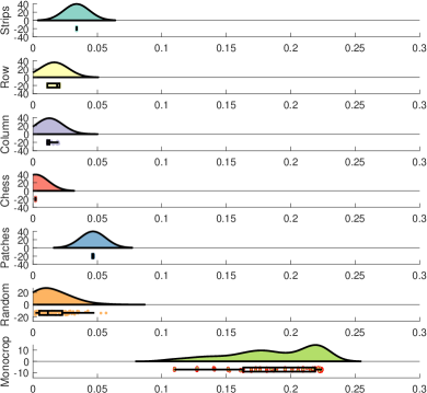
(a)

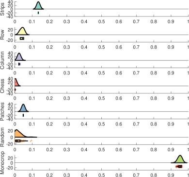
(b)

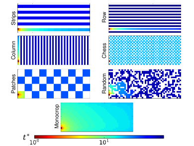
(c)

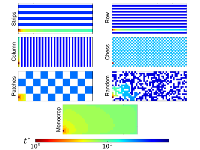
(d)

Figure 3.10: Raincloud plots of the proportion of dead plants under a SIR epidemics at $t=10$ with $\beta=0.5,$ $\mu=0.5$ for different intercropping strategies with perfect biological traps ($\gamma\rightarrow\infty$). (a) Pest with reduced mobility ($s=4.0)$ and with larger mobility ($s=2.5$) The clouds show the kernel distribution of the proportion of dead plants for different realizations of the epidemics. Below, the raw data is plotted (the rain) together with their corresponding box and whisker plots. Evolution of the propagation of a relatively low mobility pest ($s=4.0)$ (c) and of a relatively high mobility pest ($s=2.5)$ (d) across the fields. In both cases the propagation is initialized by infecting the plant on the bottom-right corner of the plot.

Supplementary Note 5

The value of the epidemic threshold $\tau$ can be obtained as the reciprocal of largest eigenvalue $\lambda_{1}\left(G\right)$ of the adjacency matrix of the network representing the arrangement:

$$\tau^{\,E}=\dfrac{1}{\lambda_{1}\left(G\right)},$$ (3.6)

Then, let $G$ be a field arrangement such that in the shortest path connecting any two arbitrary pair of susceptible plants $v_{i}$ and $v_{j}$ there is at least one trap crop. This arrangement is a subdivision of certain network $G^{\prime}$ in which a trap crop is inserted between every pair of susceptible plants. Then, let us consider the representation $G^{\prime}$ in which only the susceptible plants are represented. Every pair of susceptible plants in $G^{\prime}$ are connected by a weighted edge with a weight $\left(2d\right)^{-\gamma s}$ where $d$ is the separation, in terms of number of edges, between the two susceptible plants in the original arrangement $G$. The network $G^{\prime}$ is a weighted complete graph, in which every pair of nodes is connected by a weighted edge. Thus, if $\left(\gamma s\right)\rightarrow 0$, which is realizable having $\gamma<\infty$ and an insect pest with extremely large mobility $s\rightarrow 0$, we have that $G^{\prime}$ is a graph formed by $n/2$ nodes in which every pair of nodes is connected by an edge of weight equal to one. Consequently, the adjacency matrix is $A\left(G^{\prime}\right)=E-I$ where $E$ is the all-ones matrix and $I$ is the corresponding identity matrix. The largest eigenvalue of this matrix is $\lambda_{1}\left(G^{\prime}\right)=\dfrac{n}{2}-1.$Thus we have

$$\tau^{\,E}=\underset{n\rightarrow\infty}{\lim}\underset{\left(\gamma s\right)\rightarrow 0}{\lim}\dfrac{1}{\lambda_{1}\left(G^{\prime}\right)}=\underset{n\rightarrow\infty}{\lim}\dfrac{1}{\dfrac{n}{2}-1}=0.$$ (3.7)

That is, in very large arrangements of this type there are no epidemic threshold when the pest mobility is extremely large and the trap crop has a fixed but not infinite trap strength. This means that in this conditions just one single infestation of a plant can trigger an epidemic in the crop field.

On the other hand, let us consider that $\left(\gamma s\right)\rightarrow\infty$, which is realizable if $s>0$ and the trap crop has an extremely high strength $\gamma\rightarrow\infty$. In this case every entry of the adjacency matrix tends to zero $\left(2d\right)^{-\gamma s}\rightarrow 0$ which means that the graph representing the system is formed by $n/2$ isolated nodes. In this case we have

$$\tau^{\,E}=\underset{\left(\gamma s\right)\rightarrow\infty}{\lim}\dfrac{1}{\lambda_{1}\left(G^{\prime}\right)}=\dfrac{1}{0^{+}}=\infty.$$ (3.8)

That is, in this ideal type of intercrop arrangement in which there is one trap crop between every pair of susceptible plants it is needed to infestate an extremely large number of plants to trigger an epidemic if the strength of the trap is very high.

The previously studied ’ideal’ intercropping system is realizable by using the chessboard arrangement. That is, let us build a chessboard arrangement in which the separation between every pair of susceptible plants is larger than the radius that the insect pest has for short range dispersal. Then, we will be in a situation identical to that described by the ideal arrangement (see Supplementary Figure 3.11).

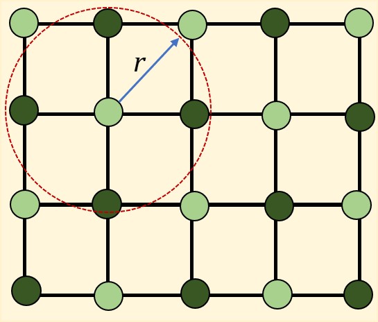
Figure 3.11: Realization of an ideal intercrop system for a crop susceptible to a pest (light green nodes) with trap crops (dark green nodes) for having extremely large epidemic threshold when the strength of the trap is very high.

References

- [1] Gerland P, Raftery AE, Ševčíková H, Li N, Gu N, Spoorenberg T, Alkema L, Fosdick BK, Chunn J, Lalic N, Bay G, Buettner T, Heilig GK, Wilmoth J. 2014 World population stabilization unlikely this century. Science 346, 234-237.
- [2] Tilman D, Balzer C, Hill J, Befort BL. 2011 Global food demand and the sustainable intensification of agriculture. Proc. Natl. Acad. Sci. 108, 20260-20264.
- [3] Tubiello FN, Soussana JF, Howden SM. 2007 Crop and pasture response to climate change. Proc. Natl. Acad. Sci. 104, 19686-19690.
- [4] Mehrabi Z, Ellis EC, Ramankutty N. 2018 The challenge of feeding the world while conserving half the planet. Nature Sustainab. 1, 409-412.
- [5] Oerke EC. 2006 Crop losses to pests. J. Agric. Sci. 144, 31-43.
- [6] Strange RN, Scott PR. 2005 Plant disease: a threat to global food security. Annu. Rev. Phytopathol. 43, 83-116.
- [7] Fisher MC, Henk DA, Briggs CJ, Brownstein JS, Madoff LC, McCraw SL, Gurr SJ. 2012 Emerging fungal threats to animal, plant and ecosystem health. Nature 484, 186-194.
- [8] Flood J. 2010 The importance of plant health to food security. Food Secur. 2, 215-231.
- [9] Chakraborty S, Newton AC. 2011 Climate change, plant diseases and food security: an overview. Plant Pathology 60, 2-14.
- [10] Khan ZR, Pickett JA, van den Berg J, Wadhams LJ, Woodcock CM. 2000 Exploiting chemical ecology and species diversity: stem borer and striga control for maize and sorghum in Africa. Pest Manag. Sci. 56, 957-962.
- [11] Bjorkman C, Niemela P. Eds. 2015 Climate Change and Insect Pests. CABI.
- [12] Thomson LJ, Macfadyen S, Hoffmann AA. 2010 Predicting the effects of climate change on natural enemies of agricultural pests. Biol. Control 52, 296-306.
- [13] Howden SM, Soussana JF, Tubiello FN, Chhetri N, Dunlop M, Meinke H. 2007 Adapting agriculture to climate change. Proc. Natl. Acad. Sci. 104, 19691-19696.
- [14] Cannon RJ. 1998 The implications of predicted climate change for insect pests in the UK, with emphasis on non-indigenous species. Global Change Biol. 4, 785-796.
- [15] Gu S, Han P, Ye Z, Perkins LE, Li J, Wang H, Zalucki M, Lu Z. 2018 Climate change favours a destructive agricultural pest in temperate regions: late spring cold matters. J. Pest Sci. 91, 1191-1198.
- [16] Rosenzweig C, Elliott J, Deryng D, Ruane AC, Müller C, Arneth A, Boote KJ, Folberth C, Glotter M, Khabarov N, Neumann K, Piontek F, Pugh TAM, Schmid E, Stehfest E, Yang H, Jones JW. 2014 Assessing agricultural risks of climate change in the 21st century in a global gridded crop model intercomparison. Proc. Natl. Acad. Sci. 111, 3268-3273.
- [17] Bebber DP, Ramotowski MA, Gurr SJ. 2013 Crop pests and pathogens move polewards in a warming world. Nature Clim. Change, 3, 985-988.
- [18] Deutsch CA, Tewksbury JJ, Tigchelaar M, Battisti DS, Merrill SC, Huey RB, Naylor RL. 2018 Increase in crop losses to insect pests in a warming climate. Science 361, 916-919.
- [19] Van Emden HF, Harrington R, Eds. 2017 Aphids as Crop Pests, Cabi International, Wallingford, U.K.
- [20] Blackman RL, Eastop VF. 2000 Aphids on the World’s Crops: An Identification and Information Guide, 2nd edn. Wiley, Chichester, UK.
- [21] Kim CS, Schaible G, Garrett L, Lubowski R, Lee D. 2008 Economic impacts of the U.S. soybean aphid infestation: a multi-regional competitive dynamic analysis. Agric. Resource Econ. Rev. 37, 227–242.
- [22] Dedryver CA, Le Ralec A, Fabre F. 2010 The conflicting relationships between aphids and men: a review of aphid damage and control strategies. Comptes Rend. Biol. 333, 539–553.
- [23] Tatchell GM. 1989 An estimate of the potential economic losses to some crops due to aphids in Britain. Crop Protect. 8, 25–29.
- [24] Hilker FM, Allen LJ, Bokil VA, Briggs CJ, Feng Z, Garrett KA, Gross LJ, Hamelin FM, Jeger MJ, Manore CA, Power AG. 2017 Modeling virus coinfection to inform management of maize lethal necrosis in Kenya. Phytopathology 107, 1095-108.
- [25] Jeger MJ, Thresh JM. 1993 Modelling reinfection of replanted cocoa by swollen shoot virus in pandemically diseased areas. J. Appl. Ecol. 1, 187-96.
- [26] Wezel A, Casagrande M, Celette F, Vian JF, Ferrer A, Peigné J. 2014 Agroecological practices for sustainable agriculture. A review. Agron. Sustain. Dev. 34, 1-20.
- [27] Muneret L, Mitchell M, Seufert V, Aviron S, Djoudi EA, Pétillon J, Plantegenest M, Thiéry D, Rusch A. 2018 Evidence that organic farming promotes pest control. Nature Sustainab. 1, 361-368.
- [28] Khan ZR, Pickett JA, Wadhams LJ, Hassanali A, Mideg CAO. 2006 Combined control of Striga hermonthica and stemborers by maize–Desmodium spp. intercrops. Crop Protect. 25, 989-995.
- [29] Smith HA, McSorley R. 2000 Intercropping and pest management: a review of major concepts. American Entomol. 46, 154-161.
- [30] Martin-Guay MO, Paquette A, Dupras J, Rivest D. 2018 The new green revolution: sustainable intensification of agriculture by intercropping. Sci. Total Environ. 615, 767-772.
- [31] Mt. Pleasant J, Burt RF. 2010 Estimating productivity of traditional Iroquoian cropping systems from field experiments and historical literature. J. Ethnobiol. 30, 52-79.
- [32] Khan, ZR, Ampong-Nyarko K, Chiliswa P, Hassanali A, Kimani S, Lwande W, Overholt WA, Overholt WA, Picketta JA, Smart LE, Woodcock CM. 1997 Intercropping increases parasitism of pests. Nature 388, 631-632.
- [33] Letourneau DK, Armbrecht I, Salguero Rivera B, Montoya Lerma J, Jiménez Carmona E, Constanza Daza M, Escobar S, Galindo V, Gutiérrez C, Duque López S, López Mejía J, Acosta Rangel AM, Herrera Rangel J, Rivera L, Saavedra CA, Torres AM, Reyes Trujillo A. 2011 Does plant diversity benefit agroecosystems? A synthetic review. Ecol. Appl. 21, 9-21.
- [34] Brooker RW, Bennett AE, Cong WF, Daniell TJ, George TS, Hallett PD, Hawes C, Iannetta PPM, Jones HG, Karley AJ, Li L, McKenzie BM, Pakeman RJ, Paterson E, Schöb C, Shen J, Squire G, Watson CA, Zhang C, Zhang F, Zhang J, White PJ. 2015 Improving intercropping: a synthesis of research in agronomy, plant physiology and ecology. New Phytologist 206, 107-117.
- [35] Brennan EB. 2016 Agronomy of strip intercropping broccoli with alyssum for biological control of aphids, Biological Control 97, 109-119.
- [36] Xu Q, Hatt S, Lopes T, Zhang Y, Bodson B, Chen J, Francis F. 2018 A push–pull strategy to control aphids combines intercropping with semiochemical releases. J. Pest Sci. 91, 93-103.
- [37] Lai R, You M, Zhu C, Gu G, Lin Z, Liao L, Lin L, Zhong X. 2017 Myzus persicae and aphid-transmitted viral disease control via variety intercropping in flue-cured tobacco. Crop Protect. 100, 157-162.
- [38] Ben-Issa R, Gomez L, Gautier H. 2017 Companion plants for aphid pest management. Insects 8, 112.
- [39] Liebhold AM, Tobin PC. 2008 Population ecology of insect invasions and their management. Ann. Rev. Entomol. 53, 387-408.
- [40] Mazzi D, Dorn S. 2012 Movement of insect pests in agricultural landscapes. Ann. Appl. Biol. 160, 97-113.
- [41] Schellhorn NA, Bianchi FJJA, Hsu CL. 2014 Movement of entomophagous arthropods in agricultural landscapes: links to pest suppression. Ann. Rev. Entomol. 59, 559-581.
- [42] Petrovskii S, Petrovskaya N, Bearup D. 2014 Multiscale approach to pest insect monitoring: random walks, pattern formation, synchronization, and networks. Phys. Life Rev. 11, 467-525.
- [43] Hethcote HW. 2000 The mathematics of infectious diseases. SIAM Rev. 42, 599-653.
- [44] Hokkanen HM. 1991 Trap cropping in pest management. Ann. Rev. Entomol. 36, 119-138.
- [45] Cook SM, Khan ZR, Pickett JA. 2007 The use of push-pull strategies in integrated pest management. Ann. Rev. Entomol. 52, 375-400.
- [46] Hassanali A, Herren H, Khan ZR, Pickett JA, Woodcock CM. 2008 Integrated pest management: the push–pull approach for controlling insect pests and weeds of cereals, and its potential for other agricultural systems including animal husbandry. Phil. Trans. Royal Soc. London B: Biol. Sci. 363, 611-621.
- [47] Pickett JA, Woodcock CM, Midega CA, Khan ZR. 2004 Push–pull farming systems. Curr. Opin. Biotech. 26, 125-132.
- [48] Xu Q, Hatt S, Lopes T, Zhang Y, Bodson B, Chen J, Francis F. 2018 A push–pull strategy to control aphids combines intercropping with semiochemical releases. J. Pest Sci. 91, 93-103.
- [49] Cooke KL. 1979Stability analysis for a vectordisease model. Rocky Mount. J. Math., 9, 31-42.
- [50] Di Liddo A. 1986 A SIR vector disease model with delay. Mat. Model. 7, 793-802.
- [51] Xu R, Ma Z. 2011 Global dynamics of a vector disease model with saturation incidence and time delay. IMA J. Appl. Math. 76, 919-937.
- [52] Tchuenche JM, Nwangwo A. 2009 Local stability of an SIR epidemic model and effect of time delay. Math. Meth. Appl. Sci. 32, 2160-2175.
- [53] Hamelin FM, Allen LJ, Prendeville HR, Hajimorad MR, Jeger MJ. 2016 The evolution of plant virus transmission pathways. J. Theor. Biol. 396, 75-89.
- [54] Jeger MJ, Madden LV, van den Bosch F. 2018 Plant virus epidemiology: Applications and prospects for mathematical modeling and analysis to improve understanding and disease control. Plant Disease 108, 837-54.
- [55] Powell G, Tosh CR, Hardie J. 2006 Host plant selection by aphids: behavioral, evolutionary, and applied perspectives. Annu. Rev. Entomol., 51, 309-330.
- [56] Kring JB. 1972 Flight behavior of aphids. Ann. Rev. .Entomol., 17, 461-492.
- [57] Norin T. 2007 Semiochemicals for insect pest management. Pure Appl. Chem. 79, 2129-2136.
- [58] Guerrieri E, Digilio MC. 2008 Aphid-plant interactions: a review. J. Plant Interact. 3, 223-232.
- [59] Diaz BM, Barrios L, Fereres A. 2012 Interplant movement and spatial distribution of alate and apterous morphs of Nasonovia ribisnigri (Homoptera: aphididae) on lettuce. Bull. Entomol. Res. 102, 406-414.
- [60] Gottlieb D, Inbar M, Lombrozo R, Ben-Ari M. 2017 Lines, loops and spirals: an intraclonal continuum of host location behaviours in walking aphids. Animal Behav. 128, 5-11.
- [61] Gish M, Inbar M. 2006 Host location by apterous aphids after escape dropping from the plant. J. Insect Behav. 19, 143-153.
- [62] Estrada E. 2012 Path Laplacian matrices: introduction and application to the analysis of consensus in networks. Lin. Algebra Appl. 436, 3373-91.
- [63] Estrada E, Hameed E, Hatano N, Langer M. 2017 Path Laplacian operators and superdiffusive processes on graphs. I. One-dimensional case. Lin. Algebra Appl. 523, 307-34.
- [64] Estrada E, Hameed E, Langer M, Puchalska A. 2018 Path Laplacian operators and superdiffusive processes on graphs. II. Two-dimensional lattice. Lin. Algebra Appl. 555, 373-97.
- [65] Pickett JA, Khan ZR. 2016 Plant volatile-mediated signalling and its application in agriculture: successes and challenges. New Phytologist 212, 856-870.
- [66] Arias, JH, Gómez-Gardeñes J, Meloni S, Estrada E. 2018 Epidemics on plants: Modeling long-range dispersal on spatially embedded networks. J. Theor. Biol. 453, 1-13.
- [67] Banks JE, Ekbom B. 1999 Modelling herbivore movement and colonozation: pest management potential of intercropping and trap cropping. Agric. Forest Entomol. 1, 165-170.
- [68] Henkel M, Hinrichsen H, Lübeck S. 2008 Non-equilibrium phase transition: Absorbing Phase Transitions (Springer Verlag).
- [69] Gómez S, Arenas A, Borge-Holthoefer J, Meloni S, Moreno Y, 2010 Discrete-time Markov chain approach to contact-based disease spreading in complex networks. EPL (Europhysics Letters) 89, 38009.
- [70] Gómez S, Gómez-Gardeñes J, Moreno Y, Arenas A, 2011. Nonperturbative heterogeneous mean-field approach to epidemic spreading in complex networks Phys. Rev. E 84, 036105.
- [71] Tajmiri P, Fathi SAA, Golizadeh A, Nouri-Ganbalani G. 2017 Effect of strip-intercropping potato and annual alfalfa on populations of Leptinotarsa decemlineata Say and its predators. Int. J. Pest Manag. 63, 273-279.
- [72] Badenes-Perez FR, Shelton AM, Nault BA. 2005 Using yellow rocket as a trap crop for diamondback moth (Lepidoptera: Plutellidae). J. Econ. Entomol. 98, 884-890.
- [73] Sheoran P, Sardana V, Singh S, Bhushan B. 2010 Bio-economic evaluation of rainfed maize (Zea mays)-based intercropping systems with blackgram (Vigna mungo) under different spatial arrangements. Indian J. Agric. Sci. 80, 244-247.
- [74] Moreira SL, Pires CV, Marcatti GE, Santos RHS, Imbuzeiro HMA, Fernandes RBA. 2018 Intercropping of coffee with the palm tree, macauba, can mitigate climate change effects. Agric. Forest Meteorol. 256, 379-390.
- [75] Estrada E, Meloni S, Sheerin M and Moreno Y. 2016 Epidemic spreading in random rectangular networks. Phys. Rev. E 94, 052316.
- [76] Allen M, Poggiali D, Whitaker K, Marshall TR, Kievit R. 2018 Raincloud plots: a multi-platform tool for robust data visualization. PeerJ Preprints, 6, e27137v1.
- [77] Mundt CC, Leonard KJ, Thal WM, Fulton JH. 1986 Computerized simulation of crown rust epidemics in mixtures of immune and susceptible oat plants with different genotype unit areas and spatial distributions of initial disease. Phytopathology 76, 590-598.
- [78] Mundt CC, Brophy LS. 1988 Influence of number of host genotype units on the effectiveness of host mixtures for disease control: a modeling approach. Phytopathology 78, 1087-1094.
- [79] Skelsey P, Rossing WA, Kessel GJ, Powell J, Van der Werf W. 2005 Influence of host diversity on development of epidemics: an evaluation and elaboration of mixture theory. Phytopathology 95, 328-38.

References

- [1] Tajmiri P, Fathi SAA, Golizadeh A, Nouri-Ganbalani G. 2017 Effect of strip-intercropping potato and annual alfalfa on populations of Leptinotarsa decemlineata Say and its predators. Int. J. Pest Manag. 63, 273-279.
- [2] Moreira SL, Pires CV, Marcatti GE, Santos RHS, Imbuzeiro HMA, Fernandes RBA. 2018 Intercropping of coffee with the palm tree, macauba, can mitigate climate change effects. Agric. Forest Meteorol. 256, 379-390.
- [3] Brooker RW, Bennett AE, Cong WF, Daniell TJ, George TS, Hallett PD, Hawes C, Iannetta PPM, Jones HG, Karley AJ, Li L, McKenzie BM, Pakeman RJ, Paterson E, Schöb C, Shen J, Squire G, Watson CA, Zhang C, Zhang F, Zhang J, White PJ. 2015 Improving intercropping: a synthesis of research in agronomy, plant physiology and ecology. New Phytologist 206, 107-117.
- [4] Martin-Guay MO, Paquette A, Dupras J, Rivest D. 2018 The new green revolution: sustainable intensification of agriculture by intercropping. Sci. Total Environ. 615, 767-772.
- [5] Estrada E. 2012 Path Laplacian matrices: introduction and application to the analysis of consensus in networks. Lin. Algebra Appl. 436, 3373-91.
- [6] Estrada E, Hameed E, Hatano N, Langer M. 2017 Path Laplacian operators and superdiffusive processes on graphs. I. One-dimensional case. Lin. Algebra Appl. 523, 307-34.
- [7] Estrada E, Hameed E, Langer M, Puchalska A. 2018 Path Laplacian operators and superdiffusive processes on graphs. II. Two-dimensional lattice. Lin. Algebra Appl. 555, 373-97.
- [8] Sheoran P, Sardana V, Singh S, Bhushan B. 2010 Bio-economic evaluation of rainfed maize (Zea mays)-based intercropping systems with blackgram (Vigna mungo) under different spatial arrangements. Indian J. Agric. Sci. 80, 244-247.
- [9] Khan ZR, Pickett JA, Wadhams LJ, Hassanali A, Mideg CAO. 2006 Combined control of Striga hermonthica and stemborers by maize–Desmodium spp. intercrops. Crop Protect. 25, 989-995.