Predicting Paleoclimate from Compositional Data using Multivariate Gaussian Process Inverse Prediction

Abstract

Multivariate compositional count data arise in many applications including ecology, microbiology, genetics, and paleoclimate. A frequent question in the analysis of multivariate compositional count data is what underlying values of a covariate(s) give rise to the observed composition. Learning the relationship between covariates and the compositional count allows for inverse prediction of unobserved covariates given compositional count observations. Gaussian processes provide a flexible framework for modeling functional responses with respect to a covariate without assuming a functional form. Many scientific disciplines use Gaussian process approximations to improve prediction and make inference on latent processes and parameters. When prediction is desired on unobserved covariates given realizations of the response variable, this is called inverse prediction. Because inverse prediction is often mathematically and computationally challenging, predicting unobserved covariates often requires fitting models that are different from the hypothesized generative model. We present a novel computational framework that allows for efficient inverse prediction using a Gaussian process approximation to generative models. Our framework enables scientific learning about how the latent processes co-vary with respect to covariates while simultaneously providing predictions of missing covariates. The proposed framework is capable of efficiently exploring the high dimensional, multi-modal latent spaces that arise in the inverse problem. To demonstrate flexibility, we apply our method in a generalized linear model framework to predict latent climate states given multivariate count data. Based on cross-validation, our model has predictive skill competitive with current methods while simultaneously providing formal, statistical inference on the underlying community dynamics of the biological system previously not available.

T1Corresponding author , , , , and

1 Introduction

A variety of data are used as proxies for climate, including tree rings, ice cores, and pollen, with each data source requiring specialized statistical methods. Therefore, improving statistical techniques for reconstructing paleoclimate from proxy data are necessary to better understand past climate. Many climate proxies are non-negative multivariate observations that occur on the unit simplex and arise when there is interest in explaining the proportion of a total. These types of data are called compositional count data and examples include fungal assays (Saucedo-Garcia et al., 2014; Grantham et al., 2015), molecular sequence data of soil microbes (Lauber et al., 2009), and paleoecological data (Haslett et al., 2006; Booth, 2008; Paciorek and McLachlan, 2009; Brewer, Jackson and Williams, 2012; Salter-Townshend and Haslett, 2012; Parnell et al., 2015). In general, compositional data are $N\times d$ counts $\mathbf{Y}$ where, for $i=1,\ldots,N$, $\mathbf{y}_{i}$ is the $d$-dimensional composition for observation $i$ (a given location or core depth) and $\sum_{j=1}^{d}y_{ij}=M_{i}$ is the total count of all species for observation $i$. When $M_{i}$ is not informative of the total abundance of the composition, these data are called compositional count data and are one of the most common sources of paleoclimate proxy data. The observed composition at site $i$ is assumed to depend on a set of covariates $\mathbf{x}_{i}$ that are only observed in the modern period and must be predicted for the past. In this manuscript, we develop novel statistical methods for generating predictions of unobserved climate $\mathbf{x}_{i}$ from observed compositional count data $\mathbf{y}_{i}$.

We present a new probabilistic model framework for paleoclimate reconstruction using compositional count data and apply our model alongside currently used Bayesian and deterministic transfer function methods to two compositional count datasets. Both of the application datasets are further subdivided into two subsets: 1) the modern calibration dataset where both the species compositions and climate variables are known and the 2) reconstruction data where only the species compositions are observed. The goal of paleoclimate reconstructions is to use the modern calibration dataset to learn model parameters and then use these parameters to predict the missing climate variables using the reconstruction data. We focus entirely on model performance for the modern calibration data because cross-validation is only possible during the modern calibration period. Therefore, we focus on the modern data only, with the assumption that models that perform well on the modern data will generalize to the reconstruction data. The two application datasets we consider are the compositional count of testate amoebae species in bogs relative to water table depth (a proxy measurement of hydroclimate) and the compositional count of pollen grains in lake sediments relative to average July temperature.

1.1 Testate Amoeba Data

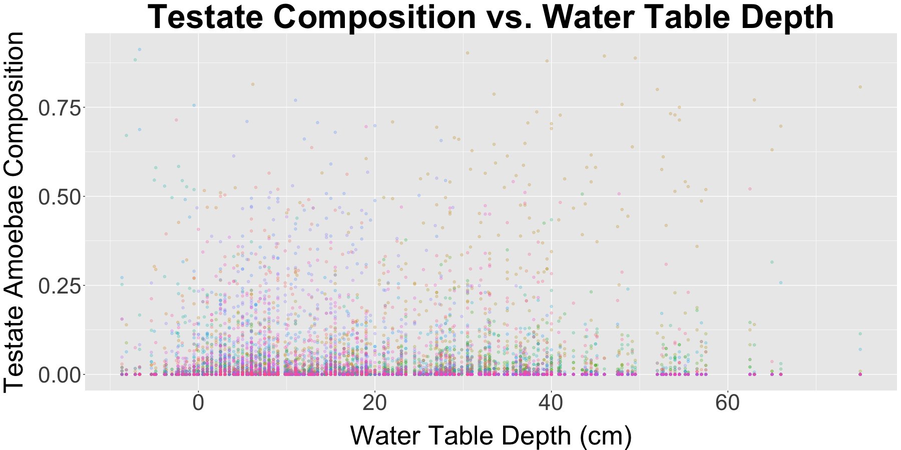
(a) Testate amoeba data.

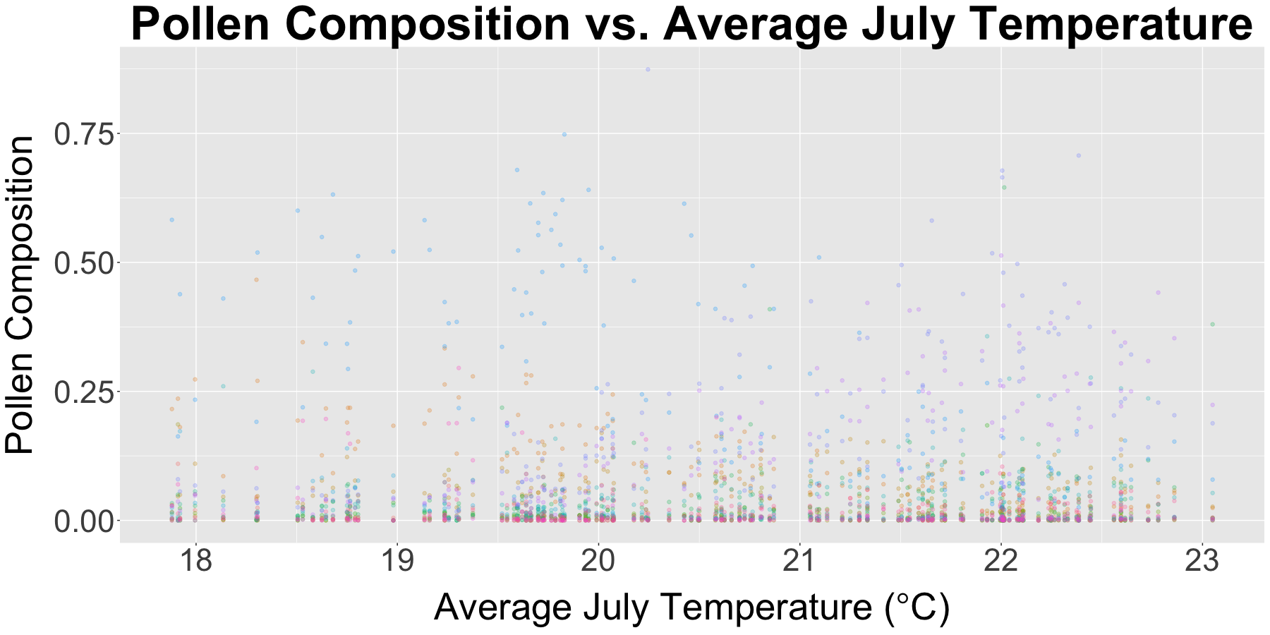
(b) Pollen data.

Figure 1: Observed data with environmental covariate along the x-axis and species counts on the y-axis. Each color represents one of the $d$ observed species. Figure (a) shows the testate amoeba data and Figure (b) shows the pollen data.

Testate amoeba are a group of protists characterized by the presence of a test (i.e., shell) which live in a range of habitats including soils, wetlands, and peat bogs. Because testate amoebae leave behind a decay-resistant test when they die and the tests can be used to identify different species of amoebae, sediment cores can be used as a record of the historical distribution of testate amoeba species. If the distribution of testate amoebae species is sensitive to environmental conditions, examination of the distribution of species through time can be used to infer past climate.

Many studies have demonstrated a sensitivity of testate amoebae from ombrotrophic peatlands to moisture conditions (i.e., water table depth) (Charman, 2007; Booth, Lamentowicz and Charman, 2010; Amesbury, Barber and Hughes, 2012). To reconstruct water table depth (in cm), we used a modern-era data set with 356 replicates of testate amoeba assemblages including 24 species along a water depth gradient (Booth, 2008). We assumed that the species compositions of testate amoebae at a given water table depth are more likely to be correlated with compositions at other bog locations with similar water table depths than nearby locations in the same bog with different water table depths. We also made the assumption that the response of testate amoebae species to water depth is fixed through time. Under these assumptions, we used the data shown in Figure 1(a) to examine the relationship between the distribution of testate amoebae and water table depth. While many studies have used testate amoebae to reconstruct water depth, much remains to be learned about the ecology of the testate amoeba communities. Important ecological questions include how the testate amoebae species respond to the underlying environment (water table depth) and how they interact.

1.2 Pollen Data

The second data source we consider is a set of pollen counts collected at 152 sites in the Upper Midwestern United States from sediments dating to the time of European settlement. The counts of pollen were identified to genus level and then grouped based on shared ecological characteristics into 16 categories. Pollen data have been studied extensively with many reconstructions of species compositions on the landscape (Dawson et al., 2016; Paciorek and McLachlan, 2009) and reconstructions of paleoclimate variables from pollen data (Wahl, Diaz and Ohlwein, 2012; Williams and Shuman, 2008; Haslett et al., 2006). We are interested in predicting temperature using the Parameter elevation Regression on Independent Slopes Model (PRISM) 30 year normal July temperature product in ^∘C (PRISM Climate Group, Oregon State University, ) as a covariate. Figure 1(b) shows the relationship between species abundances and average July temperature. We made the assumption that there is no spatial correlation in pollen counts conditional on July temperature, although the model could be expanded in future work to incorporate spatially correlated random effects.

2 Model

We begin with a brief introduction to the currently used determinisitic transfer function methods for paleoclimate reconstruction using compositional data. After introducing the most commonly used methods, we address the shortcomings of these methods to motivate the development of new probabilistic models. Next, we describe other Bayesian methods for paleoclimate reconstruction and describe the assumptions of these models that lead to the development of our model framework. We conclude this section by introducing the novel model framework and discuss how it solves many of the issues with previous methods.

2.1 Transfer function methods

The most widely used methods used in reconstructing climate from compositional data are generally known as “transfer functions.” The three transfer function methods we consider are weighted averaging (WA), the modern analog technique (MAT), and maximum likelihood response curves (MLRC). WA, MAT, and MLRC are methods that do not specify a joint likelihood for the data. WA generates reconstruction predictions by first learning parameters from the calibration data then applying those parameters to the reconstruction data. Learning model parameters from the calibration data occurs in three steps. First, WA estimates a nonparametric bootstrap distribution of “optimum” climate giving the prediction $\mu_{j}$ for species $j$ as $\hat{\mu}_{j}=\left(\sum_{i=1}^{n}y_{ij}x_{i}\right)/\left(\sum_{i=1}^{n}y_{ij}\right)$ using the modern calibration data, where $y_{ij}$ is the observed proportion of species $j$ in sample $i$ and $x_{i}$ is the climate variable for sample $i$. Second, out-of-bootstrap-sample estimates of climate $\hat{x}_{i}$ for sample $i$ are generated by taking a weighted sum of the species “optima” $\hat{x}_{i}=\frac{\sum_{j=1}^{d}y_{ij}\hat{\mu}_{j}}{\sum_{i=1}^{n}y_{ij}}$ (ter Braak and van Dam, 1989; Birks et al., 1990). The WA method induces a strong shrinkage effect because the prediction $\hat{x}_{i}$ is a mean of means. The third step in generating the calibration model corrects for this shrinkage. The shrinkage to the mean is corrected by boosting the $\hat{x}_{i}$s with either a linear or spline regression between out-of-bootstrap-sample $x_{i}$ and $\hat{x}_{i}$ resulting in a final model that is “de-shrunk” (Birks and Simpson, 2013; Schapire, 1990). The most common implementations of WA in software then summarize the bootstrap sample with the bootstrap mean and variance to generate predictions under the assumption of a normal distribution (throwing away the information in the bootstrap sample). For samples $\tilde{i}$ in the reconstruction data, predictions of paleoclimate $\hat{x}_{\tilde{i}}$ are generated using $\hat{x}_{\tilde{i}}=\frac{\sum_{j=1}^{d}y_{\tilde{i}j}\hat{\mu}_{j}}{\sum_{\tilde{i}=1}^{n}y_{\tilde{i}j}}$ with uncertainties estimated from the normal approximation to the bootstrap distribution. The uncertainty for the paleoclimate prediction can be broken down into two sources: 1) the uncertainty from the individual sample and 2) the average prediction error over the dataset. In practice, the average prediction error over the dataset dominates the uncertainty (often 95%+ of the total uncertainty in our experience). Therefore, the freqentist confidence interval widths are almost independent of the observed composition.

MAT is commonly known in the statistics and machine learning literature as $k$ nearest neighbors. For each of the $\tilde{i}$ samples in the reconstruction data, a pseudo-distance is calculated to each of the $i=1,\ldots,n$ observations in the calibration data. There are a variety of possible metrics, but the most commonly used in the literature is square chord distance (Overpeck, Webb and Prentice, 1985). The prediction $\hat{x}_{\tilde{i}}$ for samples in the reconstruction data is a (potentially weighted) average of the covariate of interest for the $k$ nearest samples in the calibration data. Confidence intervals for the MAT prediction is generated by bootstrapping the calibration data with uncertainties estimated using out-of-bootstrap-sample uncertainties and assuming a normal error distribution.

MLRC fits a curve to each marginal species component of the composition then takes a weighted average of these curves to generate a prediction. The idea behind MLRC is that, at certain ranges of the climate space, different species would have higher/lower abundance. In implementation, a logistic non-linear regression is fit to the presence/absence of each species marginally and the model predictions are made by finding the covariate value that gives rise to the highest probability of the observed composition. The simpler WA was developed to borrow the ideas of a functional response of the species to climate by reducing the computational and numerical challenges of MLRC (ter Braak and van Dam, 1989; Birks et al., 1990).

The transfer functions described above have been successful in reconstructing site-level point estimates of paleoclimate; however, transfer function methods have shortcomings. First, the transfer function methods estimate uncertainty using out-of-sample-bootstrap prediction errors that result in nearly uniform estimates of uncertainty for the reconstruction samples. This is not a desirable property because the the sample sizes used to generate the compositions change and the uncertainty estimates do not reflect the sampling intensity. In addition, there are compositions where the unobserved covariate can be predicted with higher precision than other samples based on domain knowledge, whereas current transfer functions methods are not capable of doing this. A third shortcoming is the sensitivity to compositions with zero counts; species with zero compositions are removed from the calibration dataset but sometimes the reconstruction datasets can have non-negligible counts of these species. Removing these potentially meaningful species from the analysis could have an effect on the estimation process. Finally, both WA and MLRC model the response of each species marginally, ignoring the co-dependence and covariance among the composition.

In addition, the transfer function methods each have specific issues. In WA, species that are in high abundance dominate the prediction and the prediction is less sensitive to less abundant species. For MAT, there is no clear consensus on what similarity metric is best and the final reconstruction might be sensitive to this choice. Under the “no-analog” setting (Overpeck, Webb and Webb III (1992) and Jackson and Williams (2004)) where the set of compositions are different between calibration and reconstruction datasets (i.e., there are no good “analogs” of the composition in the reconstruction data present in the calibration data because the distributions of species compositions are different), methods like WA and MAT show degraded predictive performance (Appendix S5). What makes the no-analog problem particularily nefarious is that one only uses the modern calibration data to evaluate model predictive performance leading to overly optimistic results when predictions are made using the reconstruction data. MLRC has been not widely used due to poor poor predictive performance and large confidence interval estimates - we include MLRC in our comparison as it is a likelihood-based method that serves as a methodological inspiration for our model.

Others have introduced Bayesian hierarchical models for reconstruction of paleoclimate using compositional data that overcome some of the issues with the transfer function methods. For instance, Vasko, Toivonen and Korhola (2000) introduced a Bayesian hierarchical model framework (BUMMER) to model compositional count data. BUMMER assumes that the marginal response of each species to climate follows a symmetric, unimodal Gaussian response curve. The BUMMER model uses a Dirichlet-multinomial likelihood (1) and assumes the latent random effect $\log(\alpha_{ij})$ for observation $i$ of species $j$ in (2) has the form of a Gaussian kernel

$$\log(\alpha_{ij}) =\exp\left(a_{j}-\frac{(b_{j}-x_{i})^{2}}{2c_{j}^{2}}\right),$$

where $a_{j}$ is an offset that models baseline abundance, $b_{j}$ models the mode of the symmetric, unimodal response, and $c_{j}^{2}$ is a parameter that models the spread of the functional response. In practice the data are often functional types or operational taxonomic units (OTUs) that combine many different species, each having one or more optimum responses that might respond asymmetrically to climate. Bhattacharya (2006) used a Dirichlet process mixture of unimodal Gaussian-shaped curves to model the response of each species to climate; however, the Dirichlet process approach is computationally demanding and is difficult to scale to large numbers of species. We will demonstrate that our model framework produces predictions that have similar skill to BUMMER when the symmetric, unimodal assumption is valid while greatly outperforming BUMMER predictive skill when the symmetric, unimodal assumption is violated

We introduce a novel reconstruction framework that we call the Multivariate Gaussian Process model (MVGP) in the next section. In constructing the model, we show how the MVGP model addresses the criticisms of the models described above. Another strength of the MVGP model is the ability to estimate the marginal response curves for each species as well as the correlations among the functional responses between species. Modeling inter-species correlations allows for further learning about the underlying ecology of the system as well as provides data-driven guidance on which taxa to combine together based on similar functional responses.

2.2 Compositional Data Model

Recall that compositional count data are $N\times d$ counts $\mathbf{Y}$ where, for $i=1,\ldots,N$, $\mathbf{y}_{i}$ is the $d$-dimensional composition for observation $i$ (a given location or core depth) and $\sum_{j=1}^{d}y_{ij}=M_{i}$ is the total count of all species for observation $i$. Because the data are counts, we specify the data model

$$\mathbf{y}_{i} \sim\operatorname{Multinomial}\left(M_{i},\mathbf{p}_{i}\right),$$

where the $d$-dimensional vector $\mathbf{p}_{i}\equiv\left(p_{i,1},\ldots,p_{i,d}\right)^{\prime}$ represents the probabilities of sampling species $j$ at location $i$ under the constraint $\sum_{j=1}^{d}p_{ij}=1$.

To ensure identifiability in multinomial models, one often assumes a reference category and fixes the value of the reference in the latent space. A consequence of including a reference category is that the random process $\mathbf{p}_{i}$ lives in a ($d-1$)-dimensional space. Because we are interested in allowing each species to have its own marginal response to the covariate while accounting for how these responses co-vary, we do not include a fixed reference category. In addition, visual inspection of the data and preliminary model fits suggest the compositional data are overdispersed. Therefore, we assign a mixing distribution for the probabilities $\mathbf{p}_{i}$ using the Dirichlet distribution, which allows modeling of each of the $d$ functional responses to the covariates while adding a mechanism for overdispersion.

The Dirichlet distribution is commonly used to model distributions with sum-to-one constraints, including probabilities. We assume

$$\mathbf{p}_{i} \sim\operatorname{Dirichlet}\left(\boldsymbol{\alpha}_{i}\right),$$

where the $\alpha_{ij}>0$. Because the $\boldsymbol{\alpha}_{i}$ do not have a sum-to-one constraint, we model each of the $d$ species directly using an appropriate link function. The choice of a conjugate prior model for $\mathbf{p}_{i}$ allows us to integrate out the latent variable $\mathbf{p}_{i}$, giving rise to the Dirichlet-Multinomial distribution

$$\mathbf{y}_{i} \sim\operatorname{Dirichlet-Multinomial}\left(M_{i},\boldsymbol{\alpha}_{i}\right)$$ (1)

$$=\int\operatorname{Multinomial}\left(\mathbf{y}_{i}\middle|M_{i},\mathbf{p}_{i}\right)\operatorname{Dirichlet}\left(\mathbf{p}_{i}\middle|\boldsymbol{\alpha}_{i}\right)d\,\mathbf{p}_{i}$$

where, for $i=1,\ldots,N$ independent observations of the $d$-dimensional vector $\mathbf{y}_{i}$ of counts, the data model is

$$\left[\mathbf{y}_{i}\middle|\boldsymbol{\alpha}_{i}\right]=\frac{\Gamma\left(\sum_{j=1}^{d}\alpha_{ij}\right)}{\Gamma\left(M_{i}+\sum_{j=1}^{d}\alpha_{ij}\right)}\prod_{j=1}^{d}\frac{\Gamma\left(y_{ij}+\alpha_{ij}\right)}{\Gamma\left(\alpha_{ij}\right)}.$$

To enforce the positive support of $\boldsymbol{\alpha}_{i}$, we use the log link function $\log\left(\boldsymbol{\alpha}_{i}\right)=\boldsymbol{\mu}+\boldsymbol{\zeta}_{i}+\boldsymbol{\varepsilon}_{i}$, where $\boldsymbol{\zeta}_{i}$ is a vector of random effects that is conditional on the value of the climate covariate and $\boldsymbol{\varepsilon}_{i}$ is a vector of Gaussian error that accounts for overdispersion and is uncorrelated with $\boldsymbol{\zeta}_{i}$.

2.3 Gaussian Process Model

The latent functional responses for the correlated random effect $\boldsymbol{\zeta}$ are modeled using Gaussian processes. For $i=1,\ldots,N$ replicates of the $d$-dimensional multivariate latent response $\log\left(\boldsymbol{\alpha}_{i}\right)\equiv\left(\log\left(\alpha_{i1}\right),\ldots,\log\left(\alpha_{id}\right)\right)^{\prime}$, we define the correlated multivariate Gaussian processes with nugget as

$$\log\left(\boldsymbol{\alpha}_{i}\right) =\boldsymbol{\mu}+\boldsymbol{\zeta}_{i}+\boldsymbol{\varepsilon}_{i},$$ (2)

where $\boldsymbol{\mu}$ is a vector of means and/or fixed effects. For each observation $i=1\ldots,N$, the marginal distribution of the random effect $\boldsymbol{\zeta}_{i}\equiv\left(\zeta_{i1},\ldots,\zeta_{id}\right)^{\prime}$ is mean zero Gaussian with covariance matrix $\boldsymbol{\Sigma}$ that accounts for the relationships among the observations (inter-species correlations). An important scientific question is how the $d$ functional responses co-vary across covariate space. For example, when modeling distributions of species, similar functional responses to a covariate may indicate existence of a biologically relevant functional group. Thus, inference on $\boldsymbol{\Sigma}$ allows for formal learning about the underlying ecological relationships. We assume $\boldsymbol{\varepsilon}_{i}\sim\operatorname{N}\left(\mathbf{0},\boldsymbol{\Sigma}_{\varepsilon}\right)$ is an independent and identically distributed Gaussian error vector that accounts for overdispersion in the data not explained by the Dirichlet mixture of multinomial distributions and can be added or removed from the model as necessary because it is not required for the generalized linear model.

For each dimension $j=1,\ldots,d$, the marginal random effect $\boldsymbol{\zeta}_{1:N,j}\equiv\left(\zeta_{1,j},\ldots,\zeta_{N,j}\right)^{\prime}$ is a Gaussian process with

$$\boldsymbol{\zeta}_{1:N,j} \sim\operatorname{N}\left(\mathbf{0},\mathbf{C}\left(\mathbf{X},\boldsymbol{\theta}\right)\right),$$ (3)

where $\mathbf{C}\left(\mathbf{X},\boldsymbol{\theta}\right)$ is a correlation matrix with $i,i^{\prime}$th entry $\mathbf{C}_{i,i^{\prime}}=c\left(\mathbf{x}_{i},\mathbf{x}_{i^{\prime}},\boldsymbol{\theta}\right)$ representing the latent correlation between observations at covariate values $\mathbf{x}_{i}$ and $\mathbf{x}_{i^{\prime}}$, where $\mathbf{x}_{i}$ is the $i$th row of the $N\times q$ matrix of covariates $\mathbf{X}$. Hence, we assume the joint distribution of the random effects is $\boldsymbol{\zeta}\equiv\left(\boldsymbol{\zeta_{1}}^{\prime},\ldots,\boldsymbol{\zeta}_{N}^{\prime}\right)^{\prime}\sim\operatorname{N}\left(\mathbf{0},\mathbf{C}\left(\mathbf{X},\boldsymbol{\theta}\right)\otimes\boldsymbol{\Sigma}\right)$. Each of the $d$ marginal Gaussian processes have unit variance for identifiability in the separable Kronecker product. The model can be generalized by allowing the covariance structure to be non-separable, but such extensions are not explored in this manuscript.

A common class of correlation functions is the Matérn class, of which the Gaussian and exponential correlation functions are examples (Stein, 1999). The Matérn correlation function is given by

$$c\left(\mathbf{x}_{i},\mathbf{x}_{i^{\prime}},\boldsymbol{\theta}\right) =\frac{1}{\Gamma\left(\nu\right)s^{\nu-1}}\left(\frac{2\delta_{ii^{\prime}}\sqrt{\nu}}{\rho}\right)^{\nu}\mathcal{K}_{\nu}\left(\frac{2\delta_{ii^{\prime}}\sqrt{\nu}}{\rho}\right),$$

where $\delta_{ii^{\prime}}$ is the Euclidean distance between $\mathbf{x}_{i}$ and $\mathbf{x}_{i^{\prime}}$, $\boldsymbol{\theta}=\left(\rho,\nu\right)^{\prime}$, $\rho$ is a spatial range parameter, and $\mathcal{K}_{\nu}\left(\cdot\right)$ is the modified Bessel function of the second kind with smoothness (differentiability) determined by the parameter $\nu>0$. By letting $\nu\rightarrow\infty$, the Matérn correlation function converges to the Gaussian correlation function, and setting $\nu=0.5$ results in the exponential correlation function. For the examples in this manuscript, we use the exponential correlation function

$$c\left(\mathbf{x}_{i},\mathbf{x}_{i^{\prime}},\theta\right) =\exp{\left\{-\frac{\delta_{ii^{\prime}}}{\rho}\right\}},$$

where $\theta=\rho$, although the framework accommodates arbitrary correlation functions in general.

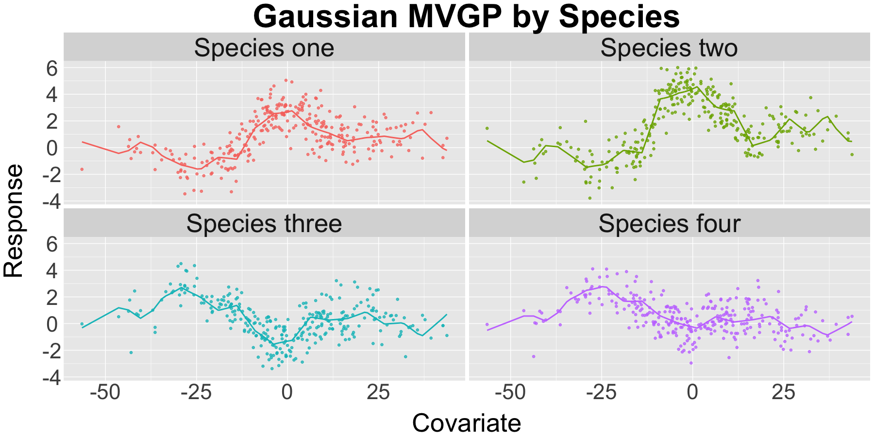
(a) Simulated Gaussian process response.

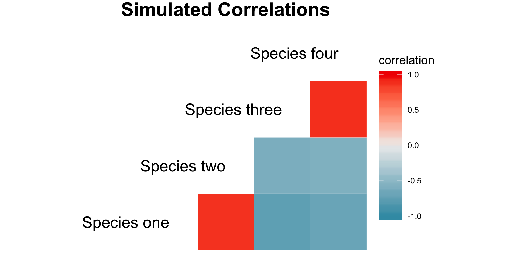
(b) Simulated correlations among species.

Figure 2: Simulation of correlated Gaussian processes for the log-scale random effect. Notice in the left figure that species one and two show a visually similar functional response to each other with respect to the covariate value, as do species three and four. The correlations are quantified by the correlation matrix on the right showing that species one and two have a positively correlated functional response, which is seen by the similarity in functional shape of the figure on the left. Likewise, species three and four have a similar functional shape and strong positive correlation. The other pairwise comparisons have different functional shapes and associated negative correlations.

An example realization of a four-dimensional correlated Gaussian process on the log-scale of the latent random effect (Figure 2(a)) shows how the log-scale random effect varies in covariate space while allowing for the different dimensions (species) of the process to co-vary. The flexible nature of the multivariate Gaussian process allows for statistical learning about both the latent functional relationships for each species and how the functional responses interact among the species. For example, Figure 2(a) shows how species one and two co-vary in their respective functional responses due to a strong positive correlation (Figure 2(b)). We can see the influence of the correlation on the Gaussian process realizations where the first and second Gaussian processes (third and fourth) have very similar shapes while the other pairwise combinations have different shapes. The similar shapes between processes one and two (three and four) are because the processes are highly correlated with pairwise correlation 0.87 (0.88). The pairwise correlations of processes one and three, one and four, two and three, and two and four are -0.76, -0.6, -0.7, and -0.57, respectively. These negative correlations indicate that these species have a different functional response to the underlying covariate relative to each other. In the ecological setting, a positive correlation in functional response could represent a relevant functional group while a negative functional correlation could represent inhibition or competition (Warton et al., 2015; Morales-Castilla et al., 2015).

We rewrite $\boldsymbol{\zeta}$ to improve computational efficiency in our MCMC algorithm. Using the upper triangular Cholesky decomposition $\boldsymbol{\Sigma}=\mathbf{R}^{\prime}\mathbf{R}$, define $\boldsymbol{\zeta}\equiv\left(\boldsymbol{\eta}_{1}^{\prime}\mathbf{R},\ldots,\boldsymbol{\eta}_{N}^{\prime}\mathbf{R}\right)^{\prime}$. For $j=1,\ldots,d$, we define

$$\boldsymbol{\eta}_{1:N,j}|c\left(\cdot,\cdot\middle|\boldsymbol{\theta}\right) \sim\operatorname{N}\left(\mathbf{0},\mathbf{C}\left(\mathbf{X},\boldsymbol{\theta}\right)\right)$$

as independent Gaussian processes and rewrite the latent process (2) on the log-scale as

$$\log\left(\boldsymbol{\alpha}_{i}\right) =\boldsymbol{\mu}+\mathbf{R}^{\prime}\boldsymbol{\eta}_{i}+\boldsymbol{\varepsilon}_{i},$$ (4)

where the marginal distribution of $\boldsymbol{\eta}_{i}\sim\operatorname{N}\left(\mathbf{0},\mathbf{I}\right)$ is multivariate standard Gaussian and the inter-species covariances are induced by the lower Cholesky matrix $\mathbf{R}$.

2.4 Prior Model

2.4.1 Prior on the missing covariates

To complete the model specification, we assign prior distributions to the remaining parameters. Because we are constructing a model for prediction of the missing, unobserved covariates given the observed covariates, we assign priors for the set of possible covariate values. For spatial and temporal problems, the support of $\mathbf{X}$ can be restricted to the domain of interest. For predictions in covariate space, the support of $\mathbf{X}$ should assign positive probability over the range of possible covariate values. We assign exchangeable priors on each of the $\tilde{i}=1,\ldots,\tilde{N}$ unobserved covariate values

$$\mathbf{x}_{\tilde{i}} \sim\operatorname{N}\left(\boldsymbol{\mu}_{X},1.5\boldsymbol{\Sigma}_{X}\right),$$ (5)

with $\boldsymbol{\mu}_{X}$ and $\boldsymbol{\Sigma}_{X}$ chosen as the sample mean and covariance of the set of observed covariates. While this prior might not be fully Bayesian (it uses the observed covariates as a prior for the unobserved covariates), we argue that, a priori, it is reasonable to assume the past values of the covariate are similar to the current values with additional variation in the past relative to current values. Other prior specifications are possible as long as the prior is Gaussian (e.g., a correlated Gaussian spatio-temporal process) because the algorithm defined in Section 2.6 leverages a Gaussian prior distribution to efficiently sample the missing covariates. We assumed the Gaussian process correlation function is isotropic, hence $c\left(\mathbf{x}_{\tilde{i}},\cdot,\boldsymbol{\theta}\right)$ depends on $\mathbf{x}_{\tilde{i}}$ only through the set of pairwise distances to all of the other $\mathbf{X}$ (both observed and unobserved). Thus, given an estimate for the distance from a location, there are possibly many potential covariate values that can have posterior probability mass, giving rise to multiple modes in the posterior (i.e., the correlation function is a many-to-one function from which we aim to generate inverse predictions). The inclusion of multiple correlated Gaussian processes helps to constrain the multimodal estimation but does not fully resolve the multimodal problem when signal to noise ratio in the data model is low. The problem is also exacerbated by a non-Gaussian likelihood associated with the compositional data. An example of the multimodal posterior distribution of the covariate is shown in Figures 3(a) and 3(b). The multimodality in the conditional posterior of $\mathbf{x}_{\tilde{i}}$ presents a challenge which requires an MCMC sampling algorithm that is capable of exploring multiple modes efficiently (hence the Gaussian prior (5), see Section 2.5 and Section 2.6 for details).

2.4.2 Prior on the covariance $\boldsymbol{\Sigma}$

The canonical inverse-Wishart prior for the covariance matrix $\boldsymbol{\Sigma}$ is often used for convenience because the inverse-Wishart is conjugate to a Gaussian likelihood, but the prior has some well-known shortcomings (Barnard, McCulloch and Meng, 2000; O’Malley and Zaslavsky, 2008). In our case, the likelihood is non-Gaussian and we do not have the computational benefits of a conjugate prior. For these reasons, we explore an alternative prior on the covariance. We use a Cholesky decomposition $\boldsymbol{\Sigma}=\mathbf{R}^{\prime}\mathbf{R}$ to induce the covariance that is vague and places marginal prior probability nearly uniformly over the space of possible correlations while assuming the marginal variances are independent of the correlations. We follow the separation strategy introduced in Barnard, McCulloch and Meng (2000) and model the marginal covariance $\boldsymbol{\Sigma}\equiv\operatorname{diag}\left(\boldsymbol{\tau}\right)\boldsymbol{\Omega}\operatorname{diag}\left(\boldsymbol{\tau}\right)$ using a diagonal matrix $\operatorname{diag}\left(\boldsymbol{\tau}\right)$ with standard deviations $\boldsymbol{\tau}=\left(\tau_{1},,\ldots,\tau_{d}\right)^{\prime}$ on the diagonal, and $\boldsymbol{\Omega}$ is an arbitrary positive definite correlation matrix. We model the upper diagonal Cholesky decomposition $\mathbf{R}_{\Omega}$ of the correlation matrix $\boldsymbol{\Omega}=\mathbf{R}_{\Omega}^{\prime}\mathbf{R}_{\Omega}$ directly, reducing computational cost by avoiding computation of the Cholesky decomposition (Pourahmadi, 1999, 2000; Smith and Kohn, 2002). Thus, we place a prior directly on the upper diagonal Cholesky matrix $\mathbf{R}=\mathbf{R}_{\Omega}\operatorname{diag}\left(\boldsymbol{\tau}\right)$ by modeling $\mathbf{R}_{\Omega}$ and $\boldsymbol{\tau}$.

Following Lewandowski, Kurowicka and Joe (2009) and the Stan Development Team (2016a), we construct a prior for the Cholesky decomposition of $\mathbf{R}_{\Omega}$ with upper diagonal elements constructed from $B={d\choose 2}$ random variables $\boldsymbol{\phi}\equiv\left(\phi_{1},\ldots,\phi_{B}\right)^{\prime}$ whose marginal support is the interval $\left(-1,1\right)$. We model the $\phi_{b}$ as independent beta random variables where, for $b=1,\ldots,B,$ $\phi_{b}\sim 2\operatorname{Beta}\left(\psi_{b},\psi_{b}\right)-1$ is a beta distribution scaled to the interval $\left(-1,1\right)$. Lewandowski, Kurowicka and Joe (2009) call $\phi_{b}$ partial correlations in a regular vine and arrange $\boldsymbol{\phi}$ in an upper triangular matrix

$$\boldsymbol{\Phi} \equiv\begin{pmatrix}0&\phi_{1}&\phi_{2}&\cdots&\phi_{B-d+2}\\ 0&0&\phi_{3}&\cdots&\phi_{B-d+3}\\ \vdots&&&\ddots&\vdots\\ 0&0&0&\cdots&\phi_{B}\\ 0&0&0&\cdots&0\\ \end{pmatrix},$$

where the $i,j$th elements of $\boldsymbol{\Phi}$ (when $i<j$) are interpreted as the correlation between the projections of the $i$th and $j$th random variables on the plane orthogonal to all variables with row index $i^{\prime}$ less than $i$. From the partial correlations $\boldsymbol{\phi}$, we construct the Cholesky factor $\mathbf{R}_{\Omega}$ using the recursive relationship (Stan Development Team, 2016a)

$$R_{\Omega{i,j}} =\begin{cases}\hfil 0&\mbox{if }i>j,\\ \hfil 1&\mbox{if }i=j=1,\\ \hfil\prod_{i^{\prime}=1}^{i-1}\sqrt{1-\Phi_{i^{\prime},j}^{2}}&\mbox{if }1<i=j,\\ \hfil\Phi_{i,j}&\mbox{if }1=i<j,\mbox{ and }\\ \hfil\Phi_{i,j}\prod_{i^{\prime}=1}^{i-1}\sqrt{1-\Phi_{i^{\prime},j}^{2}}&\mbox{if }1<i<j,\\ \end{cases},$$

where $R_{\Omega{i,j}}$ and $\Phi_{i,j}$ are the $i,j$th elements of $\mathbf{R}_{\Omega}$ and $\boldsymbol{\Phi}$, respectively.

To complete the prior on the separation model for $\boldsymbol{\Sigma}$, we follow the recommendations in Gelman (2006) and assign independent half-Cauchy priors on the standard deviations $\boldsymbol{\tau}$, where for $j=1,\ldots,d$, $\tau_{j}\sim\operatorname{half-Cauchy}\left(0,s_{j}\right)$. To sample from the half-Cauchy priors efficiently, we use the result from Armagan, Clyde and Dunson (2011) where, for $j=1,\ldots,d$, $\tau^{2}_{j}\sim\operatorname{Gamma}\left(\frac{1}{2},\lambda_{j}\right)$ with mixing parameter $\lambda_{j}\sim\operatorname{Gamma}\left(\frac{1}{2},s_{j}^{2}\right)$ inducing a half-Cauchy$\left(0,s_{j}\right)$ distribution on the standard deviation $\tau_{j}$. The prior on the uncorrelated residual error covariance $\boldsymbol{\Sigma}_{\varepsilon}$ is constructed using the same separation strategy as for $\boldsymbol{\Sigma}$. Depending on model performance in cross-validation in the generalized linear mixed model framework, the uncorrelated random effect $\boldsymbol{\varepsilon}_{i}$ can be included or dropped from the model.

2.5 Computational Considerations

When the covariates $\mathbf{X}$ are fixed and known, parameter estimation for model (2) requires on the order of $O(dN_{total}^{3})$ operations, with the computationally costly inversion and determinant of the $N_{total}\times N_{total}$ dimensional matrix $\mathbf{C}$ dominating the computation of the likelihood, where $N_{total}=N+\tilde{N}$ is the total number of locations. If $N_{total}$ is large, inversion of this matrix alone is computationally challenging. For the inverse problem, where the goal is estimation of a set of $\tilde{N}$ unknown covariates $\mathbf{x}_{\tilde{i}}$, the computational cost is prohibitive for even small $N_{total}$, because each MCMC iteration (or optimization step) over the $\tilde{N}$ missing covariates is $O(dN_{total}^{3})$ and needs to be repeated for each of the $\tilde{N}$ unobserved covariates resulting in the prohibitive computational cost of $O(\tilde{N}dN_{total}^{3})$. Thus, there is need for a computationally tractable approach for estimation under a multivariate Gaussian process model. One approach is to use a rank one Cholesky update on the full rank correlation matrix, which updates the Cholesky of the correlation matrix $\mathbf{C}$ given a single row change in $\mathbf{X}$. The rank one Cholesky update has the much lower computational cost of $O(dN_{total}^{2})$ to update the unobserved covariates because this operation uses sums of outer products of vectors, but these operations must be repeated $\tilde{N}$ times resulting in total computational complexity of $O(\tilde{N}dN_{total}^{2})+O(dN_{total}^{3})$ and we found the algorithm numerically unstable and too computationally expensive (Seeger, 2004).

A number of approaches to dimension reduction for Gaussian process models have been proposed in the literature when the goal is traditional prediction (called Kriging in the geostatistical literature), with respective advantages and disadvantages. Lindgren, Rue and Lindström (2011) proposed approximating the Gaussian process with a Markov random field by transforming the data to a regular lattice. The Gaussian Markov Random Field approach requires the space over which the Gaussian process occurs to be known, which is not appropriate for our problem. It may be possible to allow for changing locations on the lattice, but the computational difficulty in implementing this method is substantial. Another approach for reducing computational cost in Gaussian process models is to approximate the likelihood in the spectral domain (Fuentes, 2007; Paciorek, 2007; Stein, 1999). Spectral methods are difficult to implement for the traditional prediction problem, let alone for inverse prediction, because they require expert tuning and require the space over which the random process occurs to be known. Another class of methods can be described as local approximations and express the joint likelihood as a product of conditional distributions. Examples of local likelihood methods include the nearest neighbor Gaussian process (Datta et al., 2016) and the compositional likelihood introduced by Vecchia (1988). These methods suffer from issues in the inverse prediction problem because the meaning of local is ill-defined when the values over which the Gaussian process occurs are unknown.

A final class of methods for approximating Gaussian processes are linear combinations of stochastic processes, including kernel convolutions, wavelet regression, and other methods that can broadly be described as basis function expansions (Higdon, 2002; Kammann and Wand, 2003; Banerjee et al., 2008; Cressie and Johannesson, 2008; Nychka et al., 2015; Hefley et al., 2017). Basis function methods allow the random effect to be separate from the space over which the Gaussian process occurs by interpolating from a set of fixed locations, commonly referred to as knots. Instead of the location information residing in the correlation function, the information about location occurs in the basis expansion. Thus, any computation that depends on the unknown covariates requires matrix multiplication instead of matrix inversion. Although there are many different basis function models, we choose the predictive process (Banerjee et al., 2008). The predictive process approximation to the Gaussian process has the properties that the parameters of the low-rank process have the same interpretation as the parameters of the full-rank process, and the predictive process is the best low-rank approximation of order $\ell$ in terms of minimizing Kullback-Leibler divergence (Csató, 2002). Another advantage of the predictive process is that one can implement our proposed model for any arbitrary positive definite correlation function, allowing for a broad, flexible class of Gaussian process models where inverse prediction is possible.

By assuming the Gaussian process can be represented by a low-rank predictive process approximation of order $\ell$, we approximate the marginal model for the random effect (3) as

$$\boldsymbol{\eta}_{1:N,j} \approx\mathbf{c}^{\star}\left(\mathbf{X},\mathbf{X}^{\star},\boldsymbol{\theta}\right){\mathbf{C}^{\star}\left(\mathbf{X}^{\star},\boldsymbol{\theta}\right)}^{-1}\boldsymbol{\eta}_{j}^{\star}$$

$$=\mathbf{Z}\left(\mathbf{X},\mathbf{X}^{\star},\boldsymbol{\theta}\right)\boldsymbol{\eta}_{j}^{\star}$$

where $\mathbf{C}^{\star}\left(\mathbf{X}^{\star},\boldsymbol{\theta}\right)$ is the correlation matrix created by evaluating the correlation function $c\left(\mathbf{X}^{\star},\mathbf{X}^{\star},\boldsymbol{\theta}\right)$ at the $\ell$ fixed knots $\mathbf{X}^{\star}$, $\mathbf{c}^{\star}\left(\mathbf{X},\mathbf{X}^{\star}\boldsymbol{\theta}\right)=c\left(\mathbf{X},\mathbf{X}^{\star},\boldsymbol{\theta}\right)$ is the cross-correlation of the process at the covariate locations $\mathbf{X}$ and the knots $\mathbf{X}^{\star}$, $\mathbf{Z}\left(\mathbf{X},\mathbf{X}^{\star},\boldsymbol{\theta}\right)=\mathbf{c}^{\star}\left(\mathbf{X},\mathbf{X}^{\star},\boldsymbol{\theta}\right){\mathbf{C}^{\star}\left(\mathbf{X}^{\star},\mathbf{X}^{\star},\boldsymbol{\theta}\right)}^{-1}$ is the basis expansion matrix that contains known and unknown covariate values, and the low-rank random process defined at the knots is the Gaussian predictive process

$$\boldsymbol{\eta}_{j}^{\star} \sim\operatorname{N}\left(\mathbf{0},\mathbf{C}^{\star}\left(\mathbf{X}^{\star},\mathbf{X}^{\star},\boldsymbol{\theta}\right)\right).$$

Most importantly for the inverse problem, the location information (known and unknown) is in the matrix $\mathbf{Z}\left(\mathbf{X},\mathbf{X}^{\star},\boldsymbol{\theta}\right)$ rather than the correlation function. Thus, estimating the unknown Gaussian process hyperparameters requires the $O\left(d\ell^{3}\right)<<O\left(dN_{total}^{3}\right)$ inversion of the reduced-rank matrix $\mathbf{C}^{\star}\left(\mathbf{X}^{\star},\mathbf{X}^{\star},\boldsymbol{\theta}\right)$ once per MCMC iteration (this can be done using a cached Cholesky decomposition that is reused for each of the $\tilde{N}$ missing covariates) and evaluation of the likelihood for each observation with an unknown covariate is now reduced from the $O\left(dN_{total}^{3}\right)$ matrix inversion for the full model to the $O(d\ell^{2})$ vector-matrix multiplication $\mathbf{z}_{i}\boldsymbol{\eta}^{\star}$ , where $\mathbf{z}_{i}$ is the $i$th row of $\mathbf{Z}\left(\mathbf{X},\mathbf{X}^{\star},\boldsymbol{\theta}\right)$. Hence, we have reduced the computational cost from $O\left(\tilde{N}dN_{total}^{3}\right)$ to $O\left(d\ell^{3}\right)$ + $O\left(\tilde{N}d\ell^{2}\right)$. The reduced computational cost for estimating unknown covariates means the predictive process approach is well suited for our model framework, despite the predictive processes’ well-known shortcomings of producing estimates that are overly smooth at fine-scales (Finley et al., 2009; Stein, 2014).

Using the predictive process, we write our approximate Gaussian process random effect as

$$\boldsymbol{\zeta}_{i}^{\star} =\mathbf{R}^{\prime}\left(\mathbf{z}_{i}\boldsymbol{\eta}^{\star}\right)^{\prime}$$ (6)

and rewrite the latent random effect on the log-scale (4) as

$$\log\left(\boldsymbol{\alpha}_{i}\right) =\boldsymbol{\mu}+\boldsymbol{\zeta}_{i}^{\star}+\boldsymbol{\varepsilon}_{i}.$$ (7)

2.6 Implementation

The posterior we sample from using MCMC is

$$\left[\boldsymbol{\eta}^{\star},\sigma^{2},\lambda_{\sigma},\tau^{2},\lambda_{\tau},\rho,\boldsymbol{\phi},\left\{\mathbf{x}^{\prime}\right\}_{\tilde{i}=1}^{\tilde{N}}\middle|\{\mathbf{y}_{i},i=1,\ldots,N_{total}\}\right] \propto\prod_{i=1}^{N_{total}}\left[\mathbf{y}_{i}\middle|\boldsymbol{\eta}^{\star},\sigma^{2},\tau^{2},\rho\right]\left[\boldsymbol{\eta}^{\star}\middle|\tau^{2},\rho\right]\left[\sigma^{2}\middle|\lambda_{\sigma^{2}}\right]\left[\lambda_{\sigma^{2}}\right]$$

$$\hskip 17.07164pt\times\left[\tau^{2}\middle|\lambda_{\tau^{2}}\right]\left[\lambda_{\tau^{2}}\right]\left[\rho\right]\left[\boldsymbol{\phi}\right]\prod_{\tilde{i}=1}^{\tilde{N}}\left[\mathbf{x}_{\tilde{i}}\right],$$

which is high dimensional and multimodal. Thus, we develop a MCMC algorithm that is fast, efficient, and can explore a multimodal distribution effectively. The elliptical slice sampler is a highly efficient method for sampling from parameters whose prior distribution is multivariate Gaussian because the elliptical slice sampler has no tuning parameters, jointly updates parameters of interest, reduces random walk behavior, and allows for exploration of multimodal full-conditionals (Murray, Adams and MacKay, 2010). We found the elliptical slice sampler to be highly effective in sampling the high-dimensional predictive process random effect $\boldsymbol{\eta}^{\star}$ and the multimodal unobserved missing covariates $\mathbf{x}_{\tilde{i}}$; elliptical slice sampling vastly outperformed importance sampling within Gibbs and Metropolis within Gibbs algorithms (Gelfand and Smith, 1990). For other parameters, we use an adaptive random walk Metropolis within Gibbs algorithm, with multivariate proposals on the log- or logit-scale if appropriate (Roberts and Rosenthal, 2009).

All the probabilistic models were fit using 200,000 MCMC iterations, discarding the first 50,000 iterations as burn-in and fixing the adaptive proposal distributions for the remaining 150,000 iterations. Each algorithm was run for four parallel chains, thinning every 150 iterations to reduce output file size resulting in 4,000 posterior samples. Convergence was assessed using the Gelman-Rubin $\hat{R}$ statistic (Gelman et al., 1992). For the predictive process, we assign 30 knots evenly spaced over a range extending 1.5 standard deviations of the observed climate state beyond the minimum and maximum observed climate state. Based on repeated model fits, we found the inference obtained from the MVGP model to be insensitive to the number and location of knots.

To increase computational speed, we coded the algorithm in C++ using the RcppArmadillo package (Eddelbuettel and Sanderson, 2014) within the R computing environment (R Core Team, 2016b). We fit competing models in R using the rioja package (Juggins, 2015). Supplementary information, including data and code, can be found in the attached appendices and at http://github.com/jtipton25/compositional-inverse-prediction.

3 Empirical Model Evaluation

We evaluate the performance of the model framework using a simulation study as well as a cross-validation experiment using the two representative compositional count datasets. For paleoclimate proxy databases, there are often one or two environmental covariates that are measured in common across different studies. Therefore, we focus on the predictive performance of the model framework to a single covariate variable in what follows. To explore the impact of model assumptions on predictive performance we consider two simulation experiments. For the first experiment, we simulated data from the BUMMER model. The second experiment simulated data under the MVGP model. For each of these datasets, we can compare the estimates of the parameters from the equivalent simulated model to demonstrate that each model (BUMMER and MVGP) is capable of recovering the underlying simulated parameters. In addition, we can compare the influence of the symmetric, unimodal assumption of BUMMER relative to MVGP in simulated data. The simulation-based experiments evaluate predictive performance using out-of-sample test data simulated from the model under consideration. We also estimate the missing covariates using the transfer-function methods and compare with predictions generated using the proposed model. For comparisons, we also fit a simplified generalized additive model (GAM) version of the MVGP model using a B-spline approximation to the latent functional response with a Dirichlet-multinomial likelihood.

For the cross-validation experiments, we evaluate model performance using the calibration testate amoeba and pollen data. Model performance is assessed by comparing predictive skill using $k$-fold cross validation for each of the candidate models. To balance computation time and to avoid model stability issues by holding-out too much data, we cross-validated over 12-fold hold-out data sets chosen at random. All of the empirical model experiments do not include the additional overdispersion term $\boldsymbol{\varepsilon}_{i}$ as inclusion of this term did not improve predictive skill in cross-validation.

3.1 Model evaluation

We evaluated the reconstructions using mean square prediction error (MSPE), mean absolute error (MAE), empirical 95% coverage for either central Bayesian 95% credible intervals or 95% frequentist confidence intervals, and the continuous ranked probability score (CRPS) (Gneiting, 2011). One desirable property of a scoring rule is propriety. A proper scoring rule is one which, under expectation, selects the optimal predictive model. A strictly proper scoring rule is one which, under expectation, selects the optimal predictive model and no others. MSPE (MAE) has the advantage of being widely used, easy to understand, and easy to implement, but is not a strictly proper scoring rule for arbitrary likelihoods. To understand why MSPE (MAE) is not strictly proper, one can envision two models that yield the same predictive mean but different predictive variances. The best model is the one with empirical coverage closest to the nominal rate, but MSPE (MAE) is unable to distinguish between the two predictions and is thus not strictly proper. However, MSPE (MAE) is proper because the best model has the lowest score, on average. To ensure that our scores are proper, we define the point forecast as the mean (median) of the predictive distribution when using MSPE (MAE). Instead of looking at Bayesian credible interval or frequentist confidence interval coverage and MSPE or MAE jointly, one can use a strictly proper scoring rule that integrates this idea formally. CRPS is a scoring rule that rewards predictions that are close to the true value while also rewarding proper estimation of uncertainty (Gneiting, Balabdaoui and Raftery, 2007). The CRPS is defined for the cumulative predictive distribution $F$ and out-of-sample realization $y_{oos}$ as

$$CRPS\left(F,y_{oos}\right) =\int_{-\infty}^{\infty}\left(F\left(y\right)-\mathbf{I}\left(y\geq y_{oos}\right)\right)^{2}\,dy.$$

When fitting a Bayesian model using sampling methods, including MCMC, one can approximate the CRPS using

$$CRPS =\frac{1}{2K^{2}}\sum_{k=1}^{K}\sum_{\kappa=1}^{K}\left|y^{(k)}-y^{(\kappa)}\right|-\frac{1}{K}\sum_{k=1}^{K}\left|y^{(k)}-y_{oos}\right|,$$

where $y^{(k)}$ and $y^{(\kappa)}$ are the $k$th and $\kappa$th samples from the posterior predictive distribution. For the nonprobabilistic WA, MAT, and MLRC methods that produce point forecasts, the CRPS score is equivalent to MAE.

3.2 Results

Table 1: Results for predicting unobserved covariate values using simulated data. Smaller MSPE, MAE, and CRPS values indicate better model performance. Central Bayesian credible interval and frequentist confidence interval coverage values closer to the nominal 95% credible interval indicate better model performance.

(a) Simulated BUMMER data.

	CRPS	MSPE	MAE	95% CI coverage
MVGP	0.6502	1.4008	0.9105	95.0000
GAM	0.6456	1.3683	0.9121	96.0000
BUMMER	0.6397	1.3480	0.9154	93.5000
WA	1.1143	1.8814	1.1143	98.0000
MAT	1.1057	1.9993	1.1057	98.5000
MLRC	1.6331	4.3291	1.6331	100.0000

(b) Simulated MVGP data.

	CRPS	MSPE	MAE	95% CI coverage
MVGP	0.5162	1.2637	0.6793	96.0000
GAM	0.5394	1.3372	0.7113	96.5000
BUMMER	0.7198	1.7937	1.0057	96.0000
WA	1.0962	1.9467	1.0962	96.0000
MAT	0.9413	1.6814	0.9413	95.0000
MLRC	1.3245	3.3055	1.3245	95.0000

For the first simulated data experiment, the BUMMER model that assumes a symmetric, unimodal functional response of each species to climate was used to generate the data. Details about the simulation parameters can be found in Appendix S1. Predictive scores in Table 1(a) show that, for data simulated under the BUMMER model, the BUMMER model slightly outperforms MVGP and the simpler GAM across all metrics and all the probabilistic methods outperform the transfer function methods. This is unsurprising as the BUMMER model was used to simulate the data and is the correct model; however, the GAM and MVGP models produce predictions with essentially equal skill. The transfer function methods fail to perform as well as the probabilistic models under the simulated BUMMER data.

For the second simulation experiment, we simulated compositional count data from the MVGP model and generated predictions using the candidate models (Appendix S2). The results in Table 1(b) show the MVGP model performs best across all metrics with the simpler GAM model performing nearly as well. The BUMMER model shows decreased predictive skill because the symmetric, unimodal functional response assumption has been violated. The transfer function methods fail to perform as well as MVGP and GAM, with MAT outperforming WA and MLRC. The MVGP model estimated the parameters simulated from the MVGP model accurately, demonstrating that MVGP is useful for prediction and inference (Appendix S2). By providing good predictions and accurately estimating the simulated parameters in data similar to the observed data of interest, the MVGP framework is shown to be useful for both prediction and inference using the simulated data. From this experiment, we have shown that the BUMMER model shows degraded predictive performance when the assumption of a symmetric, unimodal functional response is violated.

We used 12-fold cross-validation to test model performance on the testate amoeba and pollen data to better explore the predictive performance of the candidate models. Details for the experiments can be found in Appendices S3 and S4 for the testate amoeba and pollen data, respectively. The cross-validation experiment results in Table 2(a) (testate amoeba data) and Table 2(b) (pollen data) demonstrate that the MVGP and GAM models generate the best probabilistic predictions, whereas MAT produced the best point predictions with MVGP, GAM, and WA performing similarly on these metrics. For the CRPS metric MVGP, GAM, and BUMMER are the best performing models in that order. The MAT produced confidence intervals with slightly higher than expected coverage; MVGP and GAM produced central 95% Bayesian credible intervals with lower than expected empirical coverage. In general, the cross-validated central Bayesian credible interval coverage for MVGP, GAM, and BUMMER is low for the real data sets, perhaps due to additional overdispersion that is not accounted for in the data model. The MLRC method produced the worst predictions across both studies, but is included because MLRC is a functional response method like MVGP and GAM and is robust to the no-analog problem (Appendix S5). By being competitive with currently used predictive methods, the cross-validation experiment demonstrates the potential of the MVGP inverse prediction framework for paleoclimate reconstruction. The predictions shown in Figure 3(a) and 3(b) demonstrate that the model generates reasonable predictive distributions, but the multimodality suggests that the posterior mean (or median) implied by use of MSPE (MAE) might not always a good description of the predictive distribution for MVGP and GAM - hence the decreased performance on the point prediction metrics of MSPE and MAE.

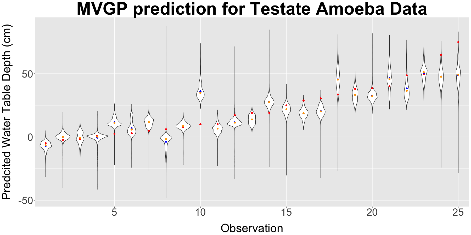
(a) Held-out testate amoeba data.

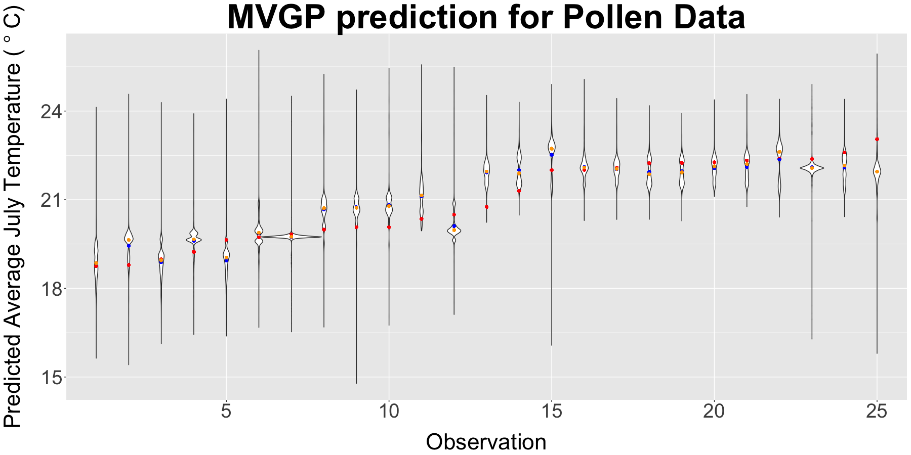
(b) Held-out pollen data.

Figure 3: 95% predictive distributions for 25 held-out observations from the testate amoeba data in Figure (a) and the pollen data in Figure (b) sorted to be increasing in the held-out covariate. The dots are at the held-out true values and the violin plots represent posterior distributions. Notice that the prediction distributions show evidence of the multimodality induced by the symmetry of the correlation function and the MCMC algorithm is capable of efficiently exploring the multiple modes. In addition, the MVGP model produces posterior distributions that have varying width for different samples.

Table 2: Cross-validation scores for experiment three using the application data. Smaller MSPE, MAE, and CRPS values indicate better model performance. Central Bayesian credible interval and frequentist confidence interval coverage values closer to the nominal 95% credible interval indicate better model performance.

(a) Testate amoeba data.

	CRPS	MSPE	MAE	95% CI coverage
MVGP	0.2959	0.2793	0.3897	78.3708
GAM	0.2966	0.2933	0.3943	79.7753
BUMMER	0.3073	0.3020	0.4077	75.8427
WA	0.4014	0.2924	0.4014	94.3820
MAT	0.3867	0.2340	0.3867	98.8764
MLRC	0.4088	0.4310	0.4088	92.6966

(b) Pollen data.

	CRPS	MSPE	MAE	95% CI coverage
MVGP	0.2746	0.2178	0.3864	87.5000
GAM	0.2828	0.2119	0.3912	78.9474
BUMMER	0.2895	0.2485	0.4001	79.6053
WA	0.3711	0.2287	0.3711	94.0789
MAT	0.3486	0.1821	0.3486	100.0000
MLRC	0.3880	0.2722	0.3880	96.7105

The MVGP, BUMMER, and GAM models also allow for inference that is not available with the transfer function methods (WA, MAT, and MLRC). The ability to make inference on the latent functional relationship between composition data and unobserved covariates is valuable. Figures 4(a) and 5(a) show the MVGP posterior mean response of each testate and pollen species to water table depth and average July temperature, respectively. Using these figures, researchers can make meaningful inference about the ecological niche that different species are exploiting. For example, in Figure 4(a) the species Assulina muscorum (assmus) is dominant in environments with water table depths deep below the peatland surface while the species Hyalosphenia elegans (hyaele) is more prevalent when water tables are near the surface. In Figure 5(a), there is a pronounced multimodal response of Pinus species to average July temperature. The Pinus taxa is a combination of different pine species that each have a different ecological niche and would be expected to have a multimodal functional response that would not be detected under the BUMMER model.

The posterior mean estimates of the correlations among functional responses shown in Figure 4(b) and Figure 5(b) provide insight into potential interactions among species. For example, some members of the same genus, such as Nebula (neb) and Assulina (ass), show positive correlations in their functional response to water depth. Not surprisingly though, there are a number of unrelated species that show high correlations, such as Trigonopyxis arcula (triarc) and Assulina spp (assmus, asssem), likely because they occupy similar niches with respect to surface moisture and other environmental conditions. This is supported in Figure 4(b) by the presence of positive correlations near the diagonal of the correlation matrix. The positive correlations near the diagonal in Figure 4(b) suggest species that have maximal responses that are near each other display a correlation in the functional response to water table depth. Importantly, species with similar energetic strategies, in particular mixotrophic species like Hyalosphenia papilio (hyapap) and Heleopera sphagni (helsph) that contain endosymbiotic zoochorellae also have high correlations, likely due to similar water-table depth tolerances as well as light requirements. Likewise Figure 5(b) shows the positive correlations of plant species with maximal responses at either the cool or hot end of the average July temperature gradient. For example, Pinus and Betula are highly correlated in their functional response, which is not surprising as these taxa frequently occur together. Species with high correlations could be clustered together in future statistical analysis to reduce the number of parameters that need to be estimated and might also save analysts time by reducing the need for taxonomic precision in some cases. These inferential questions cannot be answered by the transfer function techniques commonly used to model compositional data, demonstrating the value of the MVGP modeling approach.

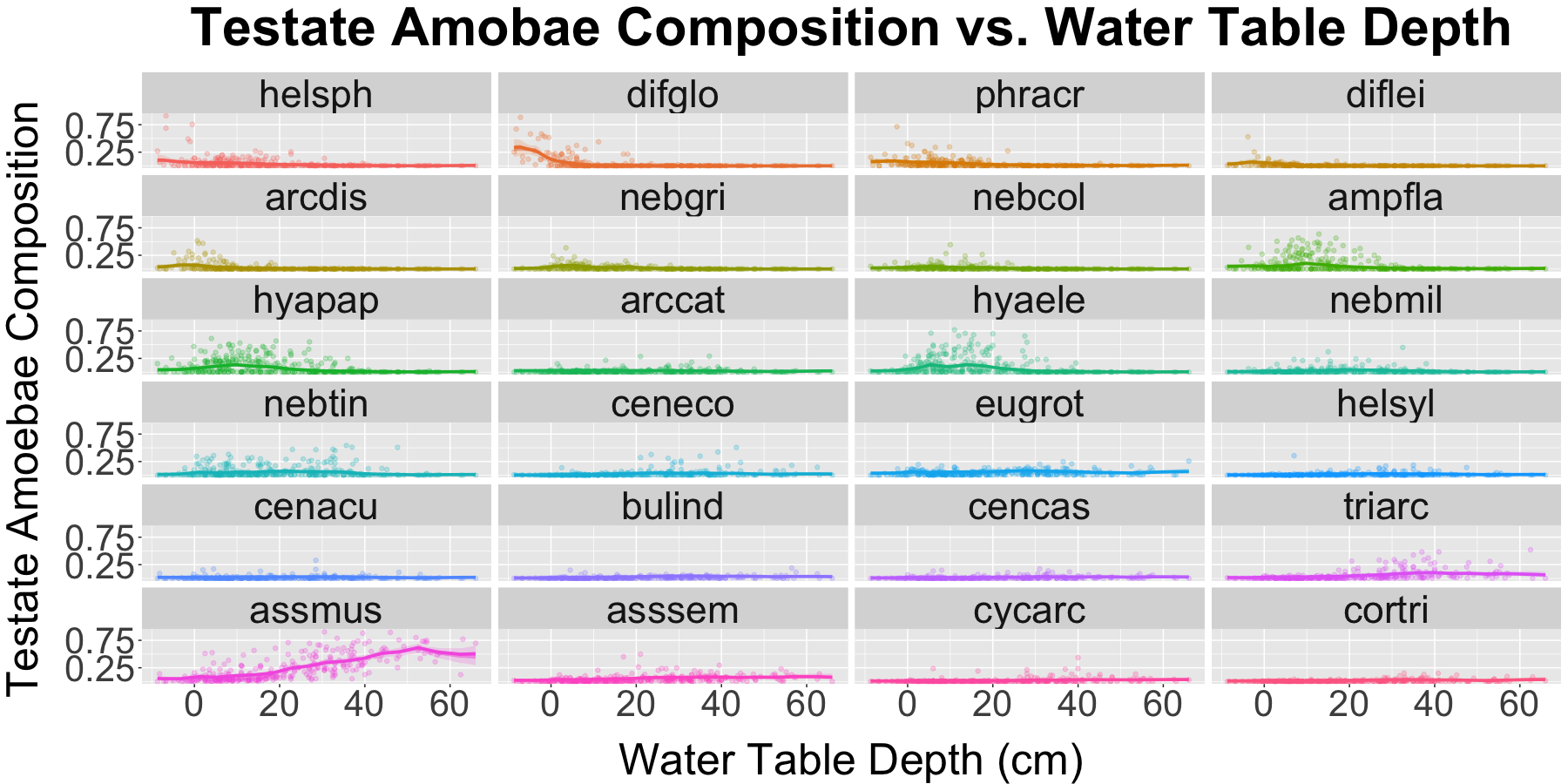
(a) Posterior mean response.

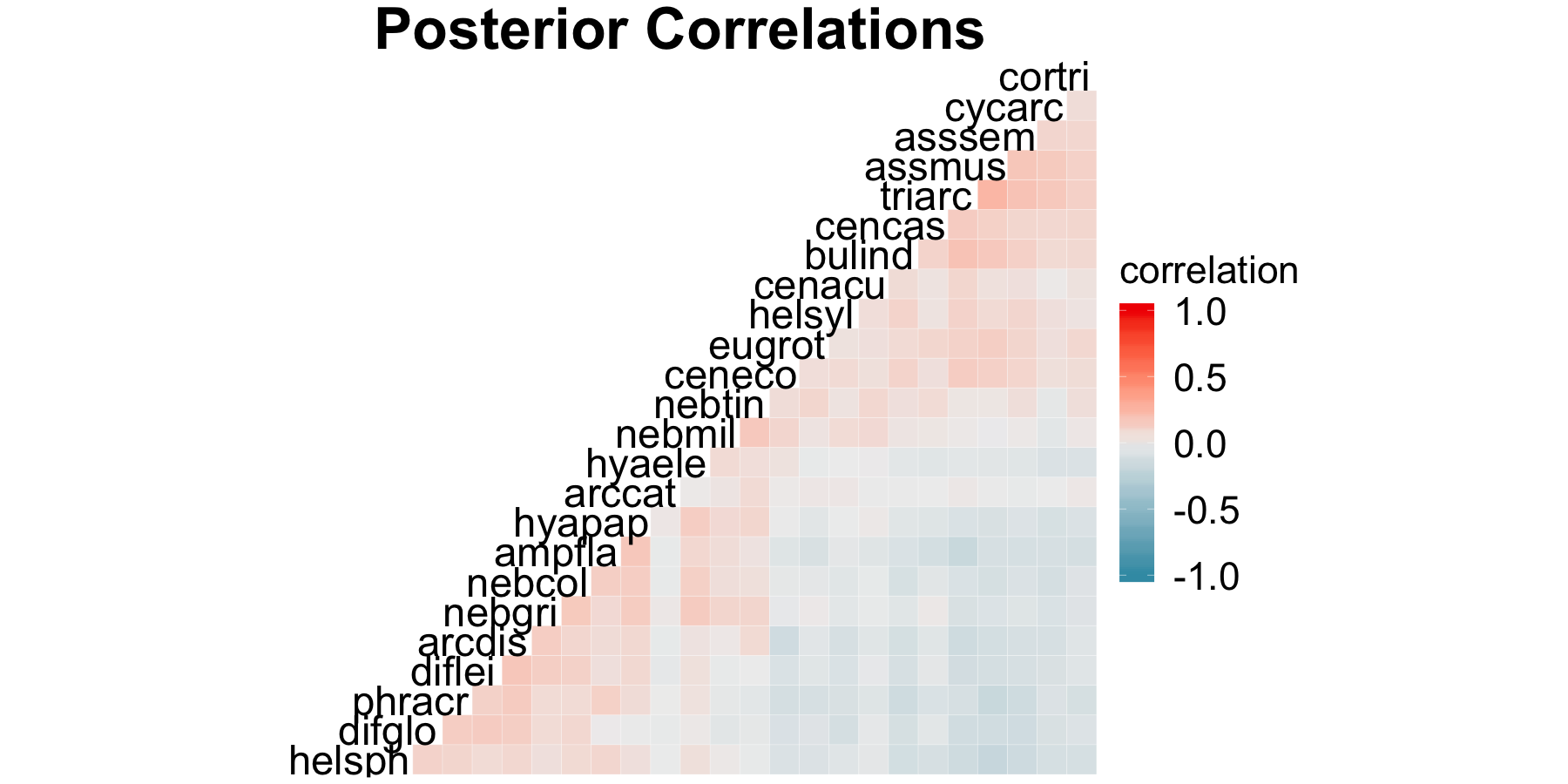
(b) Posterior Correlations.

Figure 4: Posterior model fit for the testate amoeba data. Figure (a) shows the fitted latent response of each species’ contribution to the composition with respect to water table depth, sorted by increasing maximal species response to water table depth from top left to bottom right. Figure (b) shows the posterior mean pairwise correlations in response to water table depth among testate amoeba species, sorted by increasing maximal species response to water table depth from bottom left to top right. Red colors show positive correlations and blue colors show negative correlation.

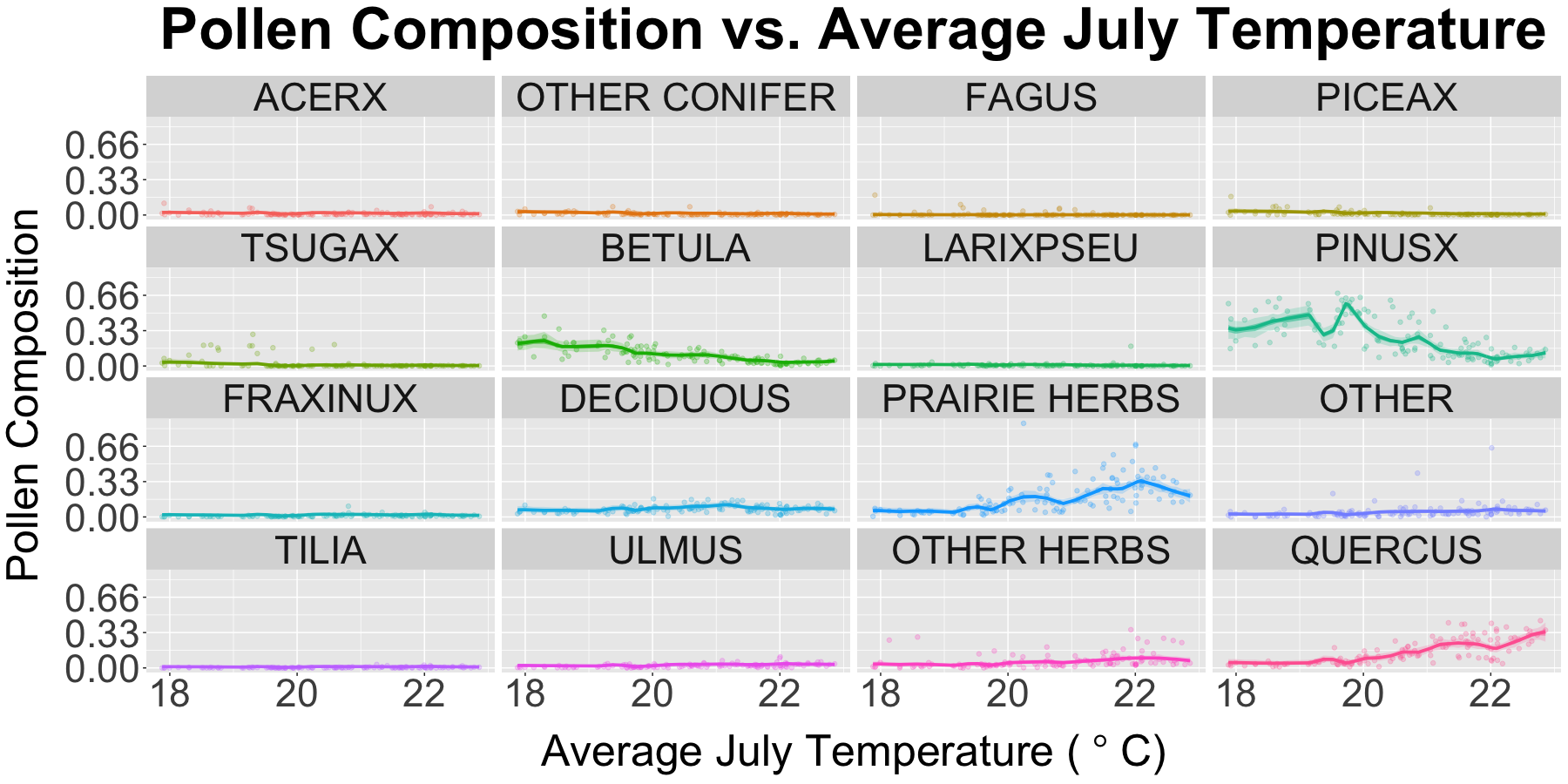
(a) Posterior mean response.

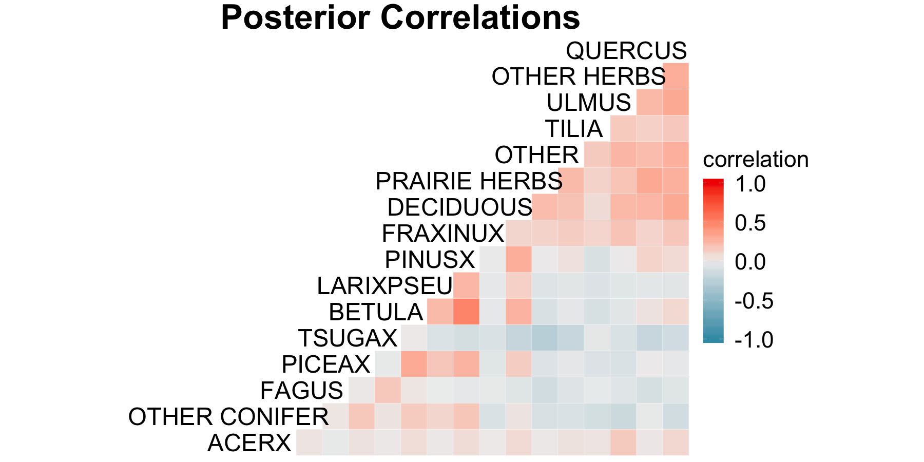
(b) Posterior Correlations.

Figure 5: Posterior model fit for the pollen data. Figure (a) shows the fitted latent response of each species’ contribution to the composition with respect to average July temperature, sorted by increasing maximal species response to temperature from top left to bottom right. Figure (b) shows the posterior mean pairwise correlations in response to average July temperature among species, sorted by increasing maximal species response to average July temperature from bottom left to top right. Red colors show positive correlations and blue colors show negative correlation.

4 Discussion

This work developed a flexible, novel model framework for prediction of unobserved climate from compositional count data. We have shown the MVGP model is capable of providing predictions that are of equal or superior skill to current methods depending on the properties of the underlying data. Although MVGP might not always be the most skilled model in cross-validation using the observed data, the MVGP model is robust to the issues commonly seen in using compositional count data to reconstruct climate including the “no-analog” setting. In “no-analog” data, the cross-validation scores for MVGP dominate the other models (Appendix S5). Thus, although MVGP does not uniformly outperform WA and MAT in cross-validation, the empirical robustness of MVGP to the “no-analog” problem (Appendix S5) and performance on data simulated from the BUMMER model suggests that our model framework is more robust to data seen in practice.

We have shown that the MVGP model can be a useful inferential tool by fitting the model to simulated data and showing that the inference accurately reproduces simulated parameters. This is important because posterior inference that we obtain from the MVGP provides learning about the underlying processes that is not available in the transfer function methods WA and MAT while making fewer assumptions than the current Bayesian methodology of BUMMER. The learning about the correlations in functional responses can be used to validate the groupings of taxa into similar functional types and provide the basis for a data-driven method of grouping taxa based on similar functional responses. Using the learning of the underlying processes giving rise to the data, we can guide future model and dataset development to iteratively improve paleoclimate reconstructions.

The statistical and computational framework developed in this manuscript allowed us to fit a complex model to compositional count data in a reasonable amount of time. We presented an algorithm for predicting unobserved inputs into a Gaussian process model by resolving a computational bottleneck that allowed for use of the highly flexible Gaussian process functional form to be used for inverse prediction. We also implemented an MCMC sampling technique that can efficiently explore the multimodal posterior generated by the inverse prediction framework.

Finally, MVGP and the other probabilistic methods for climate reconstruction have greater flexibility in future development. It is natural to extend the probabilistic models to include temporal or spatial autocorrelation by assigning the unobserved covariates $\mathbf{X}$ a correlated prior. Possible autocorrelation structures can account for either continuous or discrete observations in space and time. In addition, because the likelihood is probabilistic, one can account for radio-dating uncertainty through weighting the likelihoods using an estimated age-depth model to more fully account for uncertainty. The impact of these changes is difficult to include in a cross-validation experiment but better incorporates domain knowledge of how the climate processes evolve in time and space. Given that the MVGP model is competitive in predictive skill with current modeling efforts, the ability to extend MVGP to correlated spatio-temporal reconstructions is a great benefit. Additional improvements in reconstruction skill could also be seen by combining MVGP with other proxy data sources to provide more precise inference of paleoclimate.

5 Acknowledgements

This research is based upon work carried out by the PalEON Project (paleonproject.org) with support from the National Science Foundation MacroSystems Biology program under grant no. DEB-1241856. Any use of trade, firm, or product names is for descriptive purposes only and does not imply endorsement by the U.S. Government. Code and data found in this manuscript can be accessed at http://github.com/jtipton25/compositional-inverse-prediction.

References

- Amesbury, Barber and Hughes (2012) {barticle}[author] \bauthor\bsnmAmesbury, \bfnmMJ\binitsM., \bauthor\bsnmBarber, \bfnmKE\binitsK. and \bauthor\bsnmHughes, \bfnmPDM\binitsP. (\byear2012). \btitleThe relationship of fine-resolution, multi-proxy palaeoclimate records to meteorological data at Fågelmossen, Värmland, Sweden and the implications for the debate on climate drivers of the peat-based record. \bjournalQuaternary International \bvolume268 \bpages77–86. \endbibitem
- Armagan, Clyde and Dunson (2011) {binproceedings}[author] \bauthor\bsnmArmagan, \bfnmArtin\binitsA., \bauthor\bsnmClyde, \bfnmMerlise\binitsM. and \bauthor\bsnmDunson, \bfnmDavid B.\binitsD. B. (\byear2011). \btitleGeneralized Beta mixtures of Gaussians. In \bbooktitleAdvances in Neural Information Processing Systems \bpages523–531. \endbibitem
- Banerjee et al. (2008) {barticle}[author] \bauthor\bsnmBanerjee, \bfnmSudipto\binitsS., \bauthor\bsnmGelfand, \bfnmAlan E.\binitsA. E., \bauthor\bsnmFinley, \bfnmAndrew O.\binitsA. O. and \bauthor\bsnmSang, \bfnmHuiyan\binitsH. (\byear2008). \btitleGaussian predictive process models for large spatial data sets. \bjournalJournal of the Royal Statistical Society: Series B (Statistical Methodology) \bvolume70 \bpages825–848. \endbibitem
- Barnard, McCulloch and Meng (2000) {barticle}[author] \bauthor\bsnmBarnard, \bfnmJohn\binitsJ., \bauthor\bsnmMcCulloch, \bfnmRobert\binitsR. and \bauthor\bsnmMeng, \bfnmXiao Li\binitsX. L. (\byear2000). \btitleModeling covariance matrices in terms of standard deviations and correlations, with application to shrinkage. \bjournalStatistica Sinica \bpages1281–1311. \endbibitem
- Bhattacharya (2006) {barticle}[author] \bauthor\bsnmBhattacharya, \bfnmSourabh\binitsS. (\byear2006). \btitleA Bayesian semiparametric model for organism based environmental reconstruction. \bjournalEnvironmetrics \bvolume17 \bpages763–776. \endbibitem
- Birks and Simpson (2013) {barticle}[author] \bauthor\bsnmBirks, \bfnmH John B\binitsH. J. B. and \bauthor\bsnmSimpson, \bfnmGavin L\binitsG. L. (\byear2013). \btitle‘Diatoms and pH reconstruction’(1990) revisited. \bjournalJournal of Paleolimnology \bvolume49 \bpages363–371. \endbibitem
- Birks et al. (1990) {barticle}[author] \bauthor\bsnmBirks, \bfnmHarry J. B.\binitsH. J. B., \bauthor\bsnmLine, \bfnmJ. M.\binitsJ. M., \bauthor\bsnmJuggins, \bfnmSteve\binitsS., \bauthor\bsnmStevenson, \bfnmA. C.\binitsA. C. and \bauthor\bsnmter Braak, \bfnmCajo J. F.\binitsC. J. F. (\byear1990). \btitleDiatoms and pH reconstruction. \bjournalPhilosophical Transactions of the Royal Society of London B: Biological Sciences \bvolume327 \bpages263–278. \endbibitem
- Booth (2008) {barticle}[author] \bauthor\bsnmBooth, \bfnmRobert K.\binitsR. K. (\byear2008). \btitleTestate amoebae as proxies for mean annual water-table depth in Sphagnum-dominated peatlands of North America. \bjournalJournal of Quaternary Science \bvolume23 \bpages43–57. \endbibitem
- Booth, Lamentowicz and Charman (2010) {barticle}[author] \bauthor\bsnmBooth, \bfnmR. K.\binitsR. K., \bauthor\bsnmLamentowicz, \bfnmM\binitsM. and \bauthor\bsnmCharman, \bfnmD. J.\binitsD. J. (\byear2010). \btitlePreparation and analysis of testate amoebae in peatland paleoenvironmental studies. \bjournalMires and Peat \bvolume7 \bpages1–7. \endbibitem
- Brewer, Jackson and Williams (2012) {barticle}[author] \bauthor\bsnmBrewer, \bfnmSimon\binitsS., \bauthor\bsnmJackson, \bfnmStephen T\binitsS. T. and \bauthor\bsnmWilliams, \bfnmJohn W\binitsJ. W. (\byear2012). \btitlePaleoecoinformatics: applying geohistorical data to ecological questions. \bjournalTrends in Ecology & Evolution \bvolume27 \bpages104–112. \endbibitem
- Charman (2007) {barticle}[author] \bauthor\bsnmCharman, \bfnmDan J\binitsD. J. (\byear2007). \btitleSummer water deficit variability controls on peatland water-table changes: implications for Holocene palaeoclimate reconstructions. \bjournalThe Holocene \bvolume17 \bpages217–227. \endbibitem
- Cressie and Johannesson (2008) {barticle}[author] \bauthor\bsnmCressie, \bfnmNoel\binitsN. and \bauthor\bsnmJohannesson, \bfnmGardar\binitsG. (\byear2008). \btitleFixed rank Kriging for very large spatial data sets. \bjournalJournal of the Royal Statistical Society: Series B (Statistical Methodology) \bvolume70 \bpages209–226. \endbibitem
- Csató (2002) {bphdthesis}[author] \bauthor\bsnmCsató, \bfnmLehel\binitsL. (\byear2002). \btitleGaussian processes: iterative sparse approximations \btypePhD thesis, \bpublisherAston University. \endbibitem
- Datta et al. (2016) {barticle}[author] \bauthor\bsnmDatta, \bfnmAbhirup\binitsA., \bauthor\bsnmBanerjee, \bfnmSudipto\binitsS., \bauthor\bsnmFinley, \bfnmAndrew O\binitsA. O. and \bauthor\bsnmGelfand, \bfnmAlan E\binitsA. E. (\byear2016). \btitleHierarchical nearest-neighbor Gaussian process models for large geostatistical datasets. \bjournalJournal of the American Statistical Association \bvolume111 \bpages800–812. \endbibitem
- Dawson et al. (2016) {barticle}[author] \bauthor\bsnmDawson, \bfnmAndria\binitsA., \bauthor\bsnmPaciorek, \bfnmChristopher J\binitsC. J., \bauthor\bsnmMcLachlan, \bfnmJason S\binitsJ. S., \bauthor\bsnmGoring, \bfnmSimon\binitsS., \bauthor\bsnmWilliams, \bfnmJohn W\binitsJ. W. and \bauthor\bsnmJackson, \bfnmStephen T\binitsS. T. (\byear2016). \btitleQuantifying pollen-vegetation relationships to reconstruct ancient forests using 19th-century forest composition and pollen data. \bjournalQuaternary Science Reviews \bvolume137 \bpages156–175. \endbibitem
- Eddelbuettel and Sanderson (2014) {barticle}[author] \bauthor\bsnmEddelbuettel, \bfnmDirk\binitsD. and \bauthor\bsnmSanderson, \bfnmConrad\binitsC. (\byear2014). \btitleRcppArmadillo: Accelerating R with high-performance C++ linear algebra. \bjournalComputational Statistics and Data Analysis \bvolume71 \bpages1054–1063. \endbibitem
- Finley et al. (2009) {barticle}[author] \bauthor\bsnmFinley, \bfnmAndrew O.\binitsA. O., \bauthor\bsnmSang, \bfnmHuiyan\binitsH., \bauthor\bsnmBanerjee, \bfnmSudipto\binitsS. and \bauthor\bsnmGelfand, \bfnmAlan E.\binitsA. E. (\byear2009). \btitleImproving the performance of predictive process modeling for large datasets. \bjournalComputational Statistics & Data Analysis \bvolume53 \bpages2873–2884. \endbibitem
- Fuentes (2007) {barticle}[author] \bauthor\bsnmFuentes, \bfnmMontserrat\binitsM. (\byear2007). \btitleApproximate likelihood for large irregularly spaced spatial data. \bjournalJournal of the American Statistical Association \bvolume102 \bpages321–331. \endbibitem
- Gelfand and Smith (1990) {barticle}[author] \bauthor\bsnmGelfand, \bfnmAlan E.\binitsA. E. and \bauthor\bsnmSmith, \bfnmAdrian F. M.\binitsA. F. M. (\byear1990). \btitleSampling-based approaches to calculating marginal densities. \bjournalJournal of the American Statistical Association \bvolume85 \bpages398–409. \endbibitem
- Gelman (2006) {barticle}[author] \bauthor\bsnmGelman, \bfnmAndrew\binitsA. (\byear2006). \btitlePrior distributions for variance parameters in hierarchical models. \bjournalBayesian Analysis \bvolume1 \bpages515–533. \endbibitem
- Gelman et al. (1992) {barticle}[author] \bauthor\bsnmGelman, \bfnmAndrew\binitsA., \bauthor\bsnmRubin, \bfnmDonald B\binitsD. B. \betalet al. (\byear1992). \btitleInference from iterative simulation using multiple sequences. \bjournalStatistical science \bvolume7 \bpages457–472. \endbibitem
- Gneiting (2011) {barticle}[author] \bauthor\bsnmGneiting, \bfnmTilmann\binitsT. (\byear2011). \btitleMaking and evaluating point forecasts. \bjournalJournal of the American Statistical Association \bvolume106 \bpages746–762. \endbibitem
- Gneiting, Balabdaoui and Raftery (2007) {barticle}[author] \bauthor\bsnmGneiting, \bfnmTilmann\binitsT., \bauthor\bsnmBalabdaoui, \bfnmF.\binitsF. and \bauthor\bsnmRaftery, \bfnmA. E.\binitsA. E. (\byear2007). \btitleProbabilistic forecasts, calibration and sharpness. \bjournalJournal of the Royal Statistical Society: Series B (Statistical Methodology) \bvolume69 \bpages243–268. \endbibitem
- Grantham et al. (2015) {barticle}[author] \bauthor\bsnmGrantham, \bfnmNeal S\binitsN. S., \bauthor\bsnmReich, \bfnmBrian J\binitsB. J., \bauthor\bsnmPacifici, \bfnmKrishna\binitsK., \bauthor\bsnmLaber, \bfnmEric B\binitsE. B., \bauthor\bsnmMenninger, \bfnmHolly L\binitsH. L., \bauthor\bsnmHenley, \bfnmJessica B\binitsJ. B., \bauthor\bsnmBarberán, \bfnmAlbert\binitsA., \bauthor\bsnmLeff, \bfnmJonathan W\binitsJ. W., \bauthor\bsnmFierer, \bfnmNoah\binitsN. and \bauthor\bsnmDunn, \bfnmRobert R\binitsR. R. (\byear2015). \btitleFungi identify the geographic origin of dust samples. \bjournalPloS one \bvolume10 \bpagese0122605. \endbibitem
- Haslett et al. (2006) {barticle}[author] \bauthor\bsnmHaslett, \bfnmJohn\binitsJ., \bauthor\bsnmWhiley, \bfnmMatt\binitsM., \bauthor\bsnmBhattacharya, \bfnmSudipto\binitsS., \bauthor\bsnmSalter-Townshend, \bfnmM\binitsM., \bauthor\bsnmWilson, \bfnmSimon P\binitsS. P., \bauthor\bsnmAllen, \bfnmJRM\binitsJ., \bauthor\bsnmHuntley, \bfnmB\binitsB. and \bauthor\bsnmMitchell, \bfnmFJG\binitsF. (\byear2006). \btitleBayesian palaeoclimate reconstruction. \bjournalJournal of the Royal Statistical Society: Series A (Statistics in Society) \bvolume169 \bpages395–438. \endbibitem
- Hefley et al. (2017) {barticle}[author] \bauthor\bsnmHefley, \bfnmTrevor J\binitsT. J., \bauthor\bsnmBroms, \bfnmKristin M\binitsK. M., \bauthor\bsnmBrost, \bfnmBrian M\binitsB. M., \bauthor\bsnmBuderman, \bfnmFrances E\binitsF. E., \bauthor\bsnmKay, \bfnmShannon L\binitsS. L., \bauthor\bsnmScharf, \bfnmHenry R\binitsH. R., \bauthor\bsnmTipton, \bfnmJohn R\binitsJ. R., \bauthor\bsnmWilliams, \bfnmPerry J\binitsP. J. and \bauthor\bsnmHooten, \bfnmMevin B\binitsM. B. (\byear2017). \btitleThe basis function approach for modeling autocorrelation in ecological data. \bjournalEcology \bvolume98 \bpages632–646. \endbibitem
- Higdon (2002) {bincollection}[author] \bauthor\bsnmHigdon, \bfnmDave\binitsD. (\byear2002). \btitleSpace and space-time modeling using process convolutions. In \bbooktitleQuantitative Methods for Current Environmental Issues \bpages37–56. \bpublisherSpringer. \endbibitem
- Jackson and Williams (2004) {barticle}[author] \bauthor\bsnmJackson, \bfnmStephen T\binitsS. T. and \bauthor\bsnmWilliams, \bfnmJohn W\binitsJ. W. (\byear2004). \btitleModern analogs in Quaternary paleoecology: Here today, gone yesterday, gone tomorrow? \bjournalAnnual Review Earth Planetary Science \bvolume32 \bpages495–537. \endbibitem
- Juggins (2015) {bmanual}[author] \bauthor\bsnmJuggins, \bfnmSteve\binitsS. (\byear2015). \btitlerioja: Analysis of quaternary science data \bnoteR package version 0.9-9. \endbibitem
- Kammann and Wand (2003) {barticle}[author] \bauthor\bsnmKammann, \bfnmE. E.\binitsE. E. and \bauthor\bsnmWand, \bfnmMatthew P.\binitsM. P. (\byear2003). \btitleGeoadditive models. \bjournalJournal of the Royal Statistical Society: Series C (Applied Statistics) \bvolume52 \bpages1–18. \endbibitem
- Lauber et al. (2009) {barticle}[author] \bauthor\bsnmLauber, \bfnmChristian L\binitsC. L., \bauthor\bsnmHamady, \bfnmMicah\binitsM., \bauthor\bsnmKnight, \bfnmRob\binitsR. and \bauthor\bsnmFierer, \bfnmNoah\binitsN. (\byear2009). \btitlePyrosequencing-based assessment of soil pH as a predictor of soil bacterial community structure at the continental scale. \bjournalApplied and Environmental Microbiology \bvolume75 \bpages5111–5120. \endbibitem
- Lewandowski, Kurowicka and Joe (2009) {barticle}[author] \bauthor\bsnmLewandowski, \bfnmDaniel\binitsD., \bauthor\bsnmKurowicka, \bfnmDorota\binitsD. and \bauthor\bsnmJoe, \bfnmHarry\binitsH. (\byear2009). \btitleGenerating random correlation matrices based on vines and extended onion method. \bjournalJournal of Multivariate Analysis \bvolume100 \bpages1989–2001. \endbibitem
- Lindgren, Rue and Lindström (2011) {barticle}[author] \bauthor\bsnmLindgren, \bfnmFinn\binitsF., \bauthor\bsnmRue, \bfnmHåvard\binitsH. and \bauthor\bsnmLindström, \bfnmJohan\binitsJ. (\byear2011). \btitleAn explicit link between Gaussian fields and Gaussian Markov random fields: the stochastic partial differential equation approach. \bjournalJournal of the Royal Statistical Society: Series B (Statistical Methodology) \bvolume73 \bpages423–498. \endbibitem
- Morales-Castilla et al. (2015) {barticle}[author] \bauthor\bsnmMorales-Castilla, \bfnmIgnacio\binitsI., \bauthor\bsnmMatias, \bfnmMiguel G\binitsM. G., \bauthor\bsnmGravel, \bfnmDominique\binitsD. and \bauthor\bsnmAraújo, \bfnmMiguel B\binitsM. B. (\byear2015). \btitleInferring biotic interactions from proxies. \bjournalTrends in ecology & evolution \bvolume30 \bpages347–356. \endbibitem
- Murray, Adams and MacKay (2010) {binproceedings}[author] \bauthor\bsnmMurray, \bfnmIain\binitsI., \bauthor\bsnmAdams, \bfnmRyan Prescott\binitsR. P. and \bauthor\bsnmMacKay, \bfnmDavid J. C.\binitsD. J. C. (\byear2010). \btitleElliptical slice sampling. In \bbooktitleAISTATS \bvolume13 \bpages541–548. \endbibitem
- Nychka et al. (2015) {barticle}[author] \bauthor\bsnmNychka, \bfnmDouglas\binitsD., \bauthor\bsnmBandyopadhyay, \bfnmSoutir\binitsS., \bauthor\bsnmHammerling, \bfnmDorit\binitsD., \bauthor\bsnmLindgren, \bfnmFinn\binitsF. and \bauthor\bsnmSain, \bfnmStephan\binitsS. (\byear2015). \btitleA multiresolution Gaussian process model for the analysis of large spatial datasets. \bjournalJournal of Computational and Graphical Statistics \bvolume24 \bpages579–599. \endbibitem
- O’Malley and Zaslavsky (2008) {barticle}[author] \bauthor\bsnmO’Malley, \bfnmA. James\binitsA. J. and \bauthor\bsnmZaslavsky, \bfnmAlan M.\binitsA. M. (\byear2008). \btitleDomain-level covariance analysis for multilevel survey data with structured nonresponse. \bjournalJournal of the American Statistical Association \bvolume103 \bpages1405–1418. \endbibitem
- Overpeck, Webb and Prentice (1985) {barticle}[author] \bauthor\bsnmOverpeck, \bfnmJT\binitsJ., \bauthor\bsnmWebb, \bfnmTIII\binitsT. and \bauthor\bsnmPrentice, \bfnmIC\binitsI. (\byear1985). \btitleQuantitative interpretation of fossil pollen spectra: dissimilarity coefficients and the method of modern analogs. \bjournalQuaternary Research \bvolume23 \bpages87–108. \endbibitem
- Overpeck, Webb and Webb III (1992) {barticle}[author] \bauthor\bsnmOverpeck, \bfnmJonathan T\binitsJ. T., \bauthor\bsnmWebb, \bfnmRobert S\binitsR. S. and \bauthor\bsnmWebb III, \bfnmThompson\binitsT. (\byear1992). \btitleMapping eastern North American vegetation change of the past 18 ka: No-analogs and the future. \bjournalGeology \bvolume20 \bpages1071–1074. \endbibitem
- Paciorek (2007) {barticle}[author] \bauthor\bsnmPaciorek, \bfnmChristopher J.\binitsC. J. (\byear2007). \btitleComputational techniques for spatial logistic regression with large data sets. \bjournalComputational Statistics and Data Analysis \bvolume51 \bpages3631–3653. \endbibitem
- Paciorek and McLachlan (2009) {barticle}[author] \bauthor\bsnmPaciorek, \bfnmChristopher J.\binitsC. J. and \bauthor\bsnmMcLachlan, \bfnmJ. S.\binitsJ. S. (\byear2009). \btitleMapping ancient forests: Bayesian inference for spatio-temporal trends in forest composition using the fossil pollen proxy record. \bjournalJournal of the American Statistical Association \bvolume104 \bpages608–622. \endbibitem
- Parnell et al. (2015) {barticle}[author] \bauthor\bsnmParnell, \bfnmAndrew C\binitsA. C., \bauthor\bsnmSweeney, \bfnmJames\binitsJ., \bauthor\bsnmDoan, \bfnmThinh K\binitsT. K., \bauthor\bsnmSalter-Townshend, \bfnmMichael\binitsM., \bauthor\bsnmAllen, \bfnmJudy RM\binitsJ. R., \bauthor\bsnmHuntley, \bfnmBrian\binitsB. and \bauthor\bsnmHaslett, \bfnmJohn\binitsJ. (\byear2015). \btitleBayesian inference for palaeoclimate with time uncertainty and stochastic volatility. \bjournalJournal of the Royal Statistical Society: Series C (Applied Statistics) \bvolume64 \bpages115–138. \endbibitem
- Pourahmadi (1999) {barticle}[author] \bauthor\bsnmPourahmadi, \bfnmMohsen\binitsM. (\byear1999). \btitleJoint mean-covariance models with applications to longitudinal data: Unconstrained parameterisation. \bjournalBiometrika \bvolume86 \bpages677–690. \endbibitem
- Pourahmadi (2000) {barticle}[author] \bauthor\bsnmPourahmadi, \bfnmMohsen\binitsM. (\byear2000). \btitleMaximum likelihood estimation of generalised linear models for multivariate normal covariance matrix. \bjournalBiometrika \bvolume87 \bpages425–435. \endbibitem
- (45) {bmisc}[author] \bauthor\bsnmPRISM Climate Group, Oregon State University \bhowpublishedhttp://prism.oregonstate.edu. \bnoteCreated February 4, 2004. \endbibitem
- Roberts and Rosenthal (2009) {barticle}[author] \bauthor\bsnmRoberts, \bfnmGareth O.\binitsG. O. and \bauthor\bsnmRosenthal, \bfnmJeffrey S.\binitsJ. S. (\byear2009). \btitleExamples of adaptive MCMC. \bjournalJournal of Computational and Graphical Statistics \bvolume18 \bpages349–367. \endbibitem
- Salter-Townshend and Haslett (2012) {barticle}[author] \bauthor\bsnmSalter-Townshend, \bfnmMichael\binitsM. and \bauthor\bsnmHaslett, \bfnmJohn\binitsJ. (\byear2012). \btitleFast inversion of a flexible regression model for multivariate pollen counts data. \bjournalEnvironmetrics \bvolume23 \bpages595–605. \endbibitem
- Saucedo-Garcia et al. (2014) {barticle}[author] \bauthor\bsnmSaucedo-Garcia, \bfnmAurora\binitsA., \bauthor\bsnmAnaya, \bfnmAna Luisa\binitsA. L., \bauthor\bsnmEspinosa-Garcia, \bfnmFrancisco J\binitsF. J. and \bauthor\bsnmGonzalez, \bfnmMaria C\binitsM. C. (\byear2014). \btitleDiversity and communities of foliar endophytic fungi from different agroecosystems of Coffea arabica L. in two regions of Veracruz, Mexico. \bjournalPloS one \bvolume9 \bpagese98454. \endbibitem
- Schapire (1990) {barticle}[author] \bauthor\bsnmSchapire, \bfnmRobert E\binitsR. E. (\byear1990). \btitleThe strength of weak learnability. \bjournalMachine Learning \bvolume5 \bpages197–227. \endbibitem
- Seeger (2004) {btechreport}[author] \bauthor\bsnmSeeger, \bfnmMatthias\binitsM. (\byear2004). \btitleLow rank updates for the Cholesky decomposition. \btypeTechnical Report, \bpublisherNo. EPFL-REPORT-161468. \endbibitem
- Smith and Kohn (2002) {barticle}[author] \bauthor\bsnmSmith, \bfnmMichael\binitsM. and \bauthor\bsnmKohn, \bfnmRobert\binitsR. (\byear2002). \btitleParsimonious covariance matrix estimation for longitudinal data. \bjournalJournal of the American Statistical Association. \endbibitem
- Stein (1999) {bbook}[author] \bauthor\bsnmStein, \bfnmMichael L.\binitsM. L. (\byear1999). \btitleInterpolation of spatial data: some theory for Kriging. \bpublisherSpringer Science & Business Media. \endbibitem
- Stein (2014) {barticle}[author] \bauthor\bsnmStein, \bfnmMichael L.\binitsM. L. (\byear2014). \btitleLimitations on low rank approximations for covariance matrices of spatial data. \bjournalSpatial Statistics \bvolume8 \bpages1–19. \endbibitem
- Stan Development Team (2016a) {bmanual}[author] \bauthor\bsnmStan Development Team (\byear2016a). \btitleStan Modeling Language Users Guide and Reference Manual, \beditionversion 2.10.0 ed. \bpublisherhttp://mc-stan.org. \endbibitem
- R Core Team (2016b) {bmanual}[author] \bauthor\bsnmR Core Team (\byear2016b). \btitleR: A Language and Environment for Statistical Computing \bpublisherR Foundation for Statistical Computing, \baddressVienna, Austria. \endbibitem
- ter Braak and van Dam (1989) {barticle}[author] \bauthor\bsnmter Braak, \bfnmCajo J. F.\binitsC. J. F. and \bauthor\bsnmvan Dam, \bfnmHerman\binitsH. (\byear1989). \btitleInferring pH from diatoms: a comparison of old and new calibration methods. \bjournalHydrobiologia \bvolume178 \bpages209–223. \endbibitem
- Vasko, Toivonen and Korhola (2000) {barticle}[author] \bauthor\bsnmVasko, \bfnmKari\binitsK., \bauthor\bsnmToivonen, \bfnmHannu TT\binitsH. T. and \bauthor\bsnmKorhola, \bfnmAtte\binitsA. (\byear2000). \btitleA Bayesian multinomial Gaussian response model for organism-based environmental reconstruction. \bjournalJournal of Paleolimnology \bvolume24 \bpages243–250. \endbibitem
- Vecchia (1988) {barticle}[author] \bauthor\bsnmVecchia, \bfnmA. V.\binitsA. V. (\byear1988). \btitleEstimation and model identification for continuous spatial processes. \bjournalJournal of the Royal Statistical Society. Series B (Methodological) \bvolume50 \bpages297–312. \endbibitem
- Wahl, Diaz and Ohlwein (2012) {barticle}[author] \bauthor\bsnmWahl, \bfnmEugene R\binitsE. R., \bauthor\bsnmDiaz, \bfnmHenry F\binitsH. F. and \bauthor\bsnmOhlwein, \bfnmChristian\binitsC. (\byear2012). \btitleA pollen-based reconstruction of summer temperature in central North America and implications for circulation patterns during medieval times. \bjournalGlobal and Planetary Change \bvolume84 \bpages66–74. \endbibitem
- Warton et al. (2015) {barticle}[author] \bauthor\bsnmWarton, \bfnmDavid I\binitsD. I., \bauthor\bsnmBlanchet, \bfnmF Guillaume\binitsF. G., \bauthor\bsnmO’Hara, \bfnmRobert B\binitsR. B., \bauthor\bsnmOvaskainen, \bfnmOtso\binitsO., \bauthor\bsnmTaskinen, \bfnmSara\binitsS., \bauthor\bsnmWalker, \bfnmSteven C\binitsS. C. and \bauthor\bsnmHui, \bfnmFrancis KC\binitsF. K. (\byear2015). \btitleSo many variables: joint modeling in community ecology. \bjournalTrends in Ecology & Evolution \bvolume30 \bpages766–779. \endbibitem
- Williams and Shuman (2008) {barticle}[author] \bauthor\bsnmWilliams, \bfnmJW\binitsJ. and \bauthor\bsnmShuman, \bfnmB\binitsB. (\byear2008). \btitleObtaining accurate and precise environmental reconstructions from the modern analog technique and North American surface pollen dataset. \bjournalQuaternary Science Reviews \bvolume27 \bpages669–687. \endbibitem