Probing GHz Gravitational Waves with Graviton-magnon Resonance

Abstract

A novel method for extending the frequency frontier in gravitational wave observations is proposed. It is shown that gravitational waves can excite a magnon. Thus, gravitational waves can be probed by a graviton-magnon detector which measures resonance fluorescence of magnons. Searching for gravitational waves with a wave length $\lambda$ by using a ferromagnetic sample with a dimension $l$, the sensitivity of the graviton-magnon detector reaches spectral densities, around $5.4\times 10^{-22}\times(\frac{l}{\lambda/2\pi})^{-2}\ [{\rm Hz}^{-1/2}]$ at 14 GHz and $8.6\times 10^{-21}\times(\frac{l}{\lambda/2\pi})^{-2}\ [{\rm Hz}^{-1/2}]$ at 8.2 GHz, respectively.

I Introduction

In 2015, the gravitational wave interferometer detector LIGO Abbott et al. (2016) opened up full-blown multi-messenger astronomy and cosmology, where electromagnetic waves, gravitational waves, neutrinos, and cosmic rays are utilized to explore the universe. In future, as the history of electromagnetic wave astronomy tells us, multi-frequency gravitational wave observations will be required to boost the multi-messenger astronomy and cosmology.

The purpose of this letter is to present a novel idea for extending the frequency frontier in gravitational wave observations and to report the first limit on GHz gravitational waves. As we will see below, there are experimental and theoretical motivations to probe GHz gravitational waves.

It is useful to review the current status of gravitational wave observations Kuroda et al. (2015). It should be stressed that there exists a lowest measurable frequency. Indeed, the lowest frequency we can measure is around $10^{-18}$ Hz below which the wave length of gravitational waves exceeds the current Hubble horizon. Measuring the temperature anisotropy and the B-mode polarization of the cosmic microwave background Akrami et al. (2018); Ade et al. (2015), we can probe gravitational waves with frequencies between $10^{-18}$ Hz and $10^{-16}$ Hz. Astrometry of extragalactic radio sources is sensitive to gravitational waves with frequencies between $10^{-16}$ Hz and $10^{-9}$ Hz Gwinn et al. (1997); Darling et al. (2018). The pulsar timing arrays, like EPTA Lentati et al. (2015); Babak et al. (2016), IPTA Perera et al. (2019) and NANOGrav Arzoumanian et al. (2018), observe the gravitational waves in the frequency band from $10^{-9}$ Hz to $10^{-7}$ Hz. Doppler tracking of a space craft, which uses a measurement similar to the pulsar timing arrays, can search for gravitational waves in the frequency band from $10^{-7}$ Hz to $10^{-3}$ Hz Armstrong et al. (2003). The space interferometers LISA Amaro-Seoane et al. (2013) and DECIGO Seto et al. (2001) can cover the range between $10^{-3}$ Hz and $10$ Hz. The interferometer detectors LIGO LIG , Virgo Vir , and KAGRA Somiya (2012) with km size arm lengths can search for gravitational waves with frequencies from $10$ Hz to $1$ kHz. In this frequency band, resonant bar experiments Maggiore (2000) are complementary to the interferometers Acernese et al. (2008). Furthermore, interferometers can be used to measure gravitational waves with the frequencies between $1$ kHz and $100$ MHz. In fact, recently, the limit on gravitational waves at MHz was reported Chou et al. (2017). To our best knowledge, the measurement of $100$ MHz gravitational waves with a $0.75$ m arm length interferometer Akutsu et al. (2008) is the highest frequency gravitational wave experiment to date. Thus, the frequency range higher than $100$ MHz is remaining to be explored. Given this experimental situation, GHz experiments are desired to extend the frequency frontier.

Theoretically, GHz gravitational waves are interesting from various points of view. As is well known, inflation can produce primordial gravitational waves. Among the features of primordial gravitational waves, the most clear signature is the break of the spectrum determined by the energy scale of the inflation, which may locate at around GHz Maggiore (2000). Moreover, at the end of inflation or just after inflation, there may be a high frequency peak of gravitational waves Ito and Soda (2016); Khlebnikov and Tkachev (1997). Remarkably, there is a chance to observe non-classical nature of primordial gravitational waves with frequency between MHz and GHz Kanno and Soda (2018). On the other hand, there are many astrophysical sources producing high frequency gravitational waves Bisnovatyi-Kogan and Rudenko (2004). Among them, primordial black holes are the most interesting ones because they give a hint of the information loss problem. Exotic signals from extra dimensions may exist in the GHz band Seahra et al. (2005); Clarkson and Seahra (2007). Hence, GHz gravitational waves could be a window to the extra dimensions Ishihara and Soda (2007). Thus, it is worth investigating GHz gravitational waves to understand the astrophysical process, the early universe, and quantum gravity.

In this letter, we propose a novel method for detecting GHz gravitational waves with a magnon detector. First, we show that gravitational waves excite magnons in a ferromagnetic insulator. Furthermore, using experimental results of measurement of resonance fluorescence of magnons Crescini et al. (2018); Flower et al. (2018), we demonstrate that the sensitivity to the spectral density of gravitational waves are around $5.4\times 10^{-22}\times(\frac{l}{\lambda/2\pi})^{-2}\ [{\rm Hz}^{-1/2}]$ at 14 GHz and $8.6\times 10^{-21}\times(\frac{l}{\lambda/2\pi})^{-2}\ [{\rm Hz}^{-1/2}]$ at 8.2 GHz, respectively, where $l$ is the dimension of the ferromagnetic insulator and $\lambda$ is the wave length of the gravitational waves.

II Graviton-magnon resonance

The Dirac equation in curved spacetime with a metric $g_{\mu\nu}$ is given by

$$i\gamma^{\hat{\alpha}}e^{\mu}_{\hat{\alpha}}\left(\partial_{\mu}+\Gamma_{\mu}+ieA_{\mu}\right)\psi=m\psi\ ,$$ (1)

where $\gamma^{\hat{\alpha}}$, $e$, $A_{\mu}$ are the gamma matrices, the electronic charge, and a vector potential, respectively. A tetrad $e^{\mu}_{\hat{\alpha}}$ satisfies $e^{\hat{\alpha}}_{\mu}e^{\hat{\beta}}_{\nu}\eta_{\hat{\alpha}\hat{\beta}}=g_{\mu\nu}$. The spin connection is defined by $\Gamma_{\mu}=\frac{1}{2}e^{\hat{\alpha}}_{\nu}\sigma_{\hat{\alpha}\hat{\beta}}\left(\partial_{\mu}e^{\nu\hat{\beta}}+\Gamma^{\nu}_{\lambda\mu}e^{\lambda\hat{\beta}}\right),$ where $\sigma_{\hat{\alpha}\hat{\beta}}=\frac{1}{4}[\gamma_{\hat{\alpha}},\gamma_{\hat{\beta}}]$ is a generator of the Lorentz group and $\Gamma^{\mu}_{\nu\lambda}$ is the Christoffel symbol.

In the non-relativistic limit, one can obtain interaction terms between a magnetic field and a spin as

$$\mathcal{H}_{{\rm spin}}\simeq-\mu_{B}\left(2\delta_{ij}+h_{ij}\right)\hat{S}^{i}B^{j}\ ,$$ (2)

where $\mu_{B}=|e|/{2m}$, $\hat{\bm{S}}$, and $\bm{B}$ are the Bohr magneton, the spin of the electron, and an external magnetic field, respectively. $h_{ij}(\ll 1)$ describes “effective” gravitational waves. The second term shows that gravitational waves can interact with the spin in the presence of external magnetic fields Quach (2016).

We now consider a ferromagnetic sample which has $N$ electronic spins. Such a system is well described by the Heisenberg model:

$$\mathcal{H}_{g}=-\mu_{B}B_{z}\sum_{i}\left[2\hat{S}^{z}_{(i)}+h_{zj}\hat{S}^{j}_{(i)}\right]-\sum_{i,j}J_{ij}\hat{\bm{S}}_{(i)}\cdot\hat{\bm{S}}_{(j)}\ ,$$

(3)

where an external magnetic field $B_{z}$ is applied along the $z$-direction and $i$ specifies each of the sites of the spins. The second term represents the interactions between spins with coupling constants $J_{ij}$.

Let us consider planar gravitational waves propagating in the $z$-$x$ plane, namely, the wave number vector of the gravitational waves $\bm{k}$ has a direction $\hat{k}=(\sin\theta,0,\cos\theta)$. Moreover, we assume that the wave length of the gravitational waves is much longer than the dimension of the sample. This is the case of cavity experiments which we utilize in the next section. We can expand the metric perturbations in terms of linear polarization tensors satisfying $e^{(\sigma)}_{ij}e^{(\sigma^{\prime})}_{ij}=\delta_{\sigma\sigma^{\prime}}$ as

$$h_{ij}(t)=h^{(+)}(t)e^{(+)}_{ij}+h^{(\times)}(t)e^{(\times)}_{ij}\ ,$$ (4)

where we used the fact that the amplitude is approximately uniform over the sample. More explicitly, we took the representation

$$h^{(+)}(t)=\frac{h^{(+)}}{2}\left(e^{-iw_{h}t}+e^{iw_{h}t}\right)\ ,$$ (5)

$$h^{(\times)}(t)=\frac{h^{(\times)}}{2}\left(e^{-i(w_{h}t+\alpha)}+e^{i(w_{h}t+\alpha)}\right)\ ,$$ (6)

where $\omega_{h}$ is an angular frequency of the gravitational waves and $\alpha$ represents a difference of the phases of polarizations. Note that the polarization tensors can be explicitly constructed as

$$e_{ij}^{(+)} = \frac{1}{\sqrt{2}}\left(\begin{array}[]{ccc}\cos\theta^{2}&0&-\cos\theta\sin\theta\\ 0&-1&0\\ -\cos\theta\sin\theta&0&\sin\theta^{2}\end{array}\right),$$ (10)

$$e_{ij}^{(\times)} = \frac{1}{\sqrt{2}}\left(\begin{array}[]{ccc}0&\cos\theta&0\\ \cos\theta&0&-\sin\theta\\ 0&-\sin\theta&0\end{array}\right).$$ (14)

In the above Eqs. (10) and (14), we defined the $+$ mode as a deformation in the $y$-direction.

It is well known that the spin system (3) can be rewritten by using the Holstein-Primakoff transformation Holstein and Primakoff (1940):

$$\begin{cases}\hat{S}_{(i)}^{z}=\frac{1}{2}-\hat{C}_{i}^{\dagger}\hat{C}_{i}\ ,&\\ \hat{S}_{(i)}^{+}=\sqrt{1-\hat{C}_{i}^{\dagger}\hat{C}_{i}}\ \hat{C}_{i}\ ,&\\ \hat{S}_{(i)}^{-}=\hat{C}_{i}^{\dagger}\sqrt{1-\hat{C}_{i}^{\dagger}\hat{C}_{i}}\ ,&\end{cases}$$ (15)

where the bosonic operators $\hat{C}_{i}$ and $\hat{C}^{\dagger}_{i}$ satisfy the commutation relations $[\hat{C}_{i},\hat{C}^{\dagger}_{j}]=\delta_{ij}$ and $S_{(j)}^{\pm}=S_{(j)}^{x}\pm iS_{(j)}^{y}$ are the ladder operators. The bosonic operators describe spin waves with dispersion relations determined by $B_{z}$ and $J_{ij}$. Furthermore, provided that contributions from the surface of the sample are negligible, one can expand the bosonic operators by plane waves as

$$\hat{C}_{i}=\sum_{\bm{k}}\frac{e^{-i\bm{k}\cdot\bm{r}_{i}}}{\sqrt{N}}\hat{c}_{k}\ ,$$ (16)

where $\bm{r}_{i}$ is the position vector of the $i$ spin. The excitation of the spin waves created by $\hat{c}_{k}^{\dagger}$ is called a magnon. From now on, we only consider the uniform mode of magnons. Then from Eq. (3), using the rotating wave approximation and assuming $\hat{c}^{\dagger}\hat{c}\ll 1$, one can deduce

$$\mathcal{H}_{g}\simeq 2\mu_{B}B_{z}\hat{c}^{\dagger}\hat{c}+g_{eff}\left(\hat{c}^{\dagger}e^{-i\omega_{h}t}+\hat{c}e^{i\omega_{h}t}\right),$$ (17)

where $\hat{c}=\hat{c}_{k=0}$ and

$$g_{eff}=\frac{1}{4\sqrt{2}}\mu_{B}B_{z}\sin\theta\sqrt{N}\left[\cos^{2}\theta\,(h^{(+)})^{2}+(h^{(\times)})^{2}+2\cos\theta\sin\alpha\,h^{(+)}h^{(\times)}\right]^{1/2}\ ,$$ (18)

is an effective coupling constant between gravitational waves and a magnon. From Eq. (18), we see that the effective coupling constant has gotten a factor $\sqrt{N}$. One can also express Eq. (18) using the Stokes parameters as

$$g_{eff}=\frac{1}{4\sqrt{2}}\mu_{B}B_{z}\sin\theta\sqrt{N}\left[\frac{1+\cos^{2}\theta}{2}\,I-\frac{\sin^{2}\theta}{2}\,Q+\cos\theta\,V\right]^{1/2}\ ,$$ (19)

where the Stokes parameters for gravitational waves are defined by

$$\begin{cases}I=(h^{(+)})^{2}+(h^{(\times)})^{2}\ ,&\\ Q=(h^{(+)})^{2}-(h^{(\times)})^{2}\ ,&\\ U=2\cos\alpha\,h^{(+)}h^{(\times)}\ ,&\\ V=2\sin\alpha\,h^{(+)}h^{(\times)}\ .&\end{cases}$$ (20)

They satisfy $I^{2}=U^{2}+Q^{2}+V^{2}$. We see that the effective coupling constant depends on the polarizations. Note that the Stokes parameters $Q$ and $U$ transform as

$$\binom{Q^{\prime}}{U^{\prime}}=\begin{pmatrix}\cos 4\Psi&\sin 4\Psi\\ -\sin 4\Psi&\cos 4\Psi\end{pmatrix}\binom{Q}{U}$$ (21)

where $\Psi$ is the rotation angle around $\bm{k}$.

The second term in Eq. (17) shows that planar gravitational waves induce the resonant spin precessions if the angular frequency of the gravitational waves is near the Lamor frequency, $2\mu_{B}B_{z}$. It is worth noting that the situation is similar to the resonant bar experiments Maggiore (2000) where planar gravitational waves excite phonons in a bar detector.

In the next section, utilizing the graviton-magnon resonance, we will give upper limits on GHz gravitational waves.

III Limits on GHz gravitational waves

In the previous section, we showed that planar gravitational waves can induce resonant spin precession of electrons. It is our observation that the same resonance is caused by coherent oscillation of the axion dark matter Barbieri et al. (1989). Recently, measurements of resonance fluorescence of magnons induced by the axion dark matter was conducted and upper bounds on an axion-electron coupling constant have been obtained Crescini et al. (2018); Flower et al. (2018). The point is that we can utilize these experimental results to give the upper bounds on the amplitude of GHz gravitational waves.

Actually, the interaction hamiltonian which describe an axion-magnon resonance is given by

$$\mathcal{H}_{a}=\tilde{g}_{eff}\left(\hat{c}^{\dagger}e^{-im_{a}t}+\hat{c}e^{im_{a}t}\right)\ ,$$ (22)

where $\tilde{g}_{eff}$ is an effective coupling constant between an axion and a magnon. Notice that the axion oscillates with a frequency determined by the axion mass $m_{a}$. One can see that this form is the same as the interaction term in Eq. (17). Through the hamiltonian (22), $\tilde{g}_{eff}$ is related to an axion-electron coupling constant in Crescini et al. (2018); Flower et al. (2018). Then the axion-electron coupling constant can be converted to $\tilde{g}_{eff}$ by using parameters, such as the energy density of the axion dark matter, which are explicitly given in Crescini et al. (2018); Flower et al. (2018). Therefore constraints on $\tilde{g}_{eff}$ (95% C.L.) can be read from the constraints on the axion-electron coupling constant given in Crescini et al. (2018) and Flower et al. (2018), respectively, as follows:

$$\tilde{g}_{eff}<\begin{cases}3.5\times 10^{-12}\ {\rm eV}\ ,&\\ 3.1\times 10^{-11}\ {\rm eV}\ .&\end{cases}$$ (23)

It is easy to convert the above constraints to those on the amplitude of gravitational waves appearing in the effective coupling constant (19). Indeed, we can read off the external magnetic field $B_{z}$ and the number of electrons $N$ as $(B_{z},N)=(0.5\,{\rm T},\ 5.6\times 10^{19})$ from Crescini et al. (2018) and $(B_{z},N)=(0.3\,{\rm T},\ 9.2\times 10^{19})$ from Flower et al. (2018), respectively. The external magnetic field $B_{z}$ determines the frequency of gravitational waves we can detect. Therefore, using Eqs. (19), (23) and the above parameters, one can put upper limits on gravitational waves at frequencies determined by $B_{z}$. Since Crescini et al. (2018) and Flower et al. (2018) focused on the direction of Cygnus and set the external magnetic fields to be perpendicular to it, we probe continuous gravitational waves coming from Cygnus with $\theta=\frac{\pi}{2}$ (more precisely, $\sin\theta=0.9$ in Flower et al. (2018)). We also assume there to be no linear and circular polarizations, i.e., $Q^{\prime}=U^{\prime}=V=0$. Consequently, experimental data Crescini et al. (2018) and Flower et al. (2018) show the sensitivity to the characteristic amplitude of gravitational waves defined by $h_{c}=h^{(+)}=h^{(\times)}$ as

$$h_{c}\sim\begin{cases}9.1\times 10^{-17}\times(\frac{l}{\lambda/2\pi})^{-2}\quad{\rm at}\ 14\ {\rm GHz}\ ,&\\ 1.1\times 10^{-15}\times(\frac{l}{\lambda/2\pi})^{-2}\quad{\rm at}\ 8.2\ {\rm GHz}\ ,&\end{cases}$$ (24)

respectively. Note that a suppression factor $(\frac{l}{\lambda/2\pi})^{2}\sim 10^{-3}$ has appeared (see the footnote 1). In terms of the spectral density defined by $S_{h}=h_{c}^{2}/2f$ and the energy density parameter defined by $\Omega_{GW}=2\pi^{2}f^{2}h_{c}^{2}/3H_{0}^{2}$ ($H_{0}$ is the Hubble parameter), the sensitivities are

$$\sqrt{S_{h}}\sim\begin{cases}5.4\times 10^{-22}\times(\frac{l}{\lambda/2\pi})^{-2}\ [{\rm Hz}^{-1/2}]\quad{\rm at}\ 14\ {\rm GHz}\ ,&\\ 8.6\times 10^{-21}\times(\frac{l}{\lambda/2\pi})^{-2}\ [{\rm Hz}^{-1/2}]\quad{\rm at}\ 8.2\ {\rm GHz}\ .&\end{cases}$$ (25)

and

$$h_{0}^{2}\Omega_{GW}\sim\begin{cases}1.1\times 10^{23}\times(\frac{l}{\lambda/2\pi})^{-2}\quad{\rm at}\ 14\ {\rm GHz}\ ,&\\ 5.3\times 10^{24}\times(\frac{l}{\lambda/2\pi})^{-2}\quad{\rm at}\ 8.2\ {\rm GHz}\ .&\end{cases}$$ (26)

We depicted the sensitivity on the spectral density with several other gravitational wave experiments in Fig. 1.

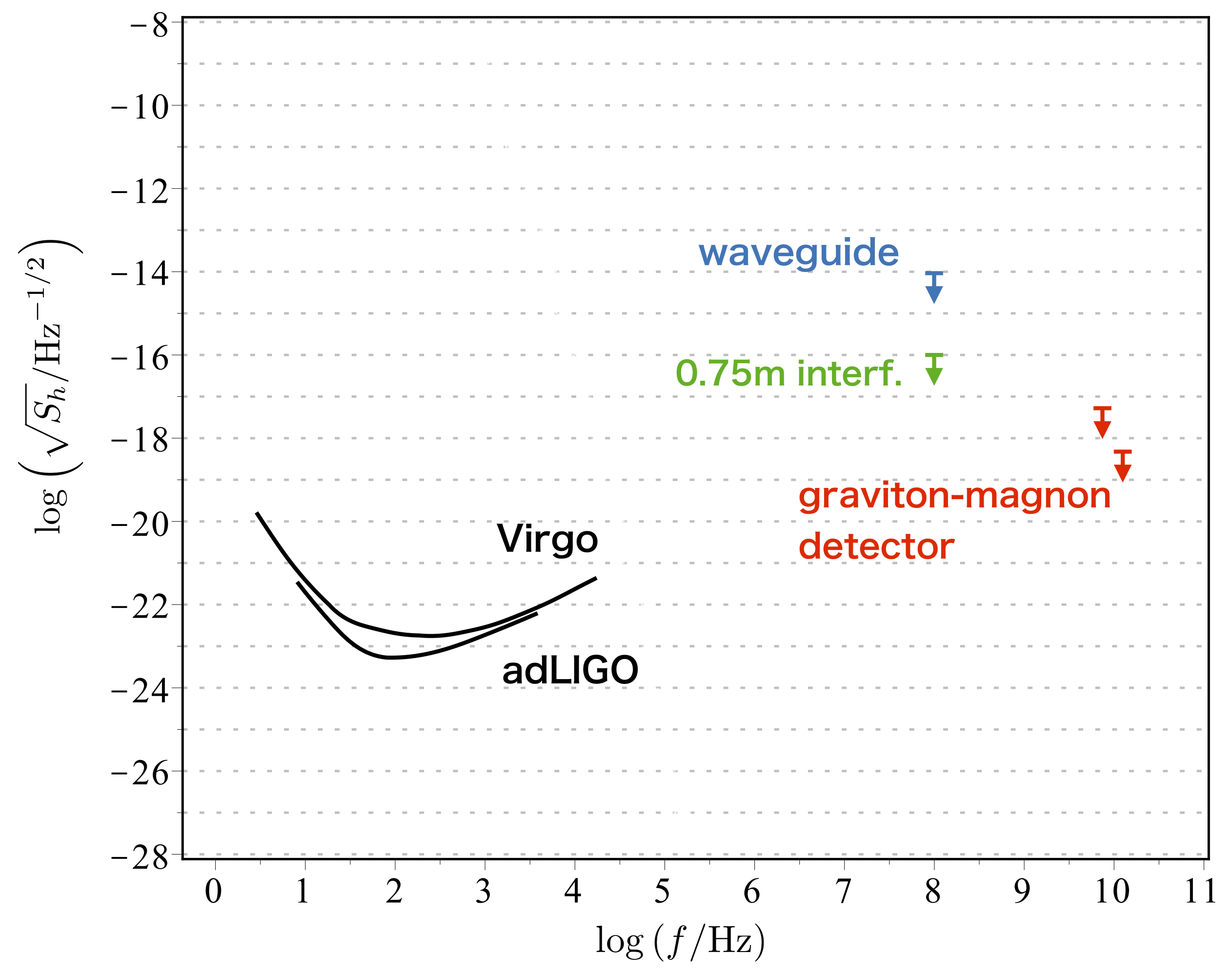
Figure 1: Several experimental sensitivities and constraints on high frequency gravitational waves are depicted. LIGO and Virgo have the sensitivity around $10^{2}$ Hz LIG ; Vir . The blue color represents an upper limit on stochastic gravitational waves by waveguide experiment using an interaction between electromagnetic fields and gravitational waves Cruise and Ingley (2006). The green one is the upper limit on stochastic gravitational waves, obtained by the 0.75 m interferometer Akutsu et al. (2008). The red color represents the sensitivity of the graviton-magnon detector.

IV Discussion

In this letter, we focused on continuous gravitational waves as an explicit demonstration to show the sensitivity of our new gravitational wave detection method as summarized in Fig. 1. Interestingly, there are several theoretical models predicting high frequency gravitational waves which are within the scope of our method Kuroda et al. (2015). The graviton-magnon resonance is also useful for probing stochastic gravitational waves with almost the same sensitivity illustrated in Fig. 1. Although the current sensitivity is still not sufficient for putting a meaningful constraint on stochastic gravitational waves, it is important to pursue the high frequency stochastic gravitational wave search for future gravitational wave physics. Moreover, we can probe burst gravitational waves of any wave form if the duration time is smaller than the relaxation time of a system. The situation is the same as for resonant bar detectors Maggiore (2007); Astone et al. (2010). For instance, in the measurements Crescini et al. (2018); Flower et al. (2018), the relaxation time is about $0.1$ $\upmu$s which is determined by the line width of the ferromagnetic sample and the cavity. If the duration of a burst of gravitational waves is smaller than $0.1$ $\upmu$s, we can detect it. Furthermore, improving the line width of the sample and the cavity not only leads to detecting burst gravitational waves but also to increasing the sensitivity. As another way to improve sensitivity, quantum nondemolition measurement may be promising Tabuchi et al. (2015, 2016); Lachance-Quirion et al. (2017). In particular, although we assumed that a gravitational wave was approximately monochromatic, there might be cases where the approximation is not valid. In such cases, quantum nondemolition measurement would be useful.

V Conclusion

Given the importance of extending the frequency frontier in gravitational wave observations, we proposed a novel method to detect GHz gravitational waves with the magnon detector. Indeed, gravitational waves can excite a magnon. Using experimental results for the axion dark matter search, Crescini et al. (2018) and Flower et al. (2018), we showed that the sensitivity to the spectral density of continuous gravitational waves reaches around $5.4\times 10^{-22}\times(\frac{l}{\lambda/2\pi})^{-2}\ [{\rm Hz}^{-1/2}]$ at 14 GHz and $8.6\times 10^{-21}\times(\frac{l}{\lambda/2\pi})^{-2}\ [{\rm Hz}^{-1/2}]$ at 8.2 GHz, respectively. One can perform all sky search of continuous gravitational waves at the above sensitivity with the graviton-magnon detector. We can also search for stochastic gravitational waves and burst gravitational waves with almost the same sensitivity.