Financial Applications of Gaussian Processes and Bayesian Optimization

Abstract

In the last five years, the financial industry has been impacted by the emergence of digitalization and machine learning. In this article, we explore two methods that have undergone rapid development in recent years: Gaussian processes and Bayesian optimization. Gaussian processes can be seen as a generalization of Gaussian random vectors and are associated with the development of kernel methods. Bayesian optimization is an approach for performing derivative-free global optimization in a small dimension, and uses Gaussian processes to locate the global maximum of a black-box function. The first part of the article reviews these two tools and shows how they are connected. In particular, we focus on the Gaussian process regression, which is the core of Bayesian machine learning, and the issue of hyperparameter selection. The second part is dedicated to two financial applications. We first consider the modeling of the term structure of interest rates. More precisely, we test the fitting method and compare the GP prediction and the random walk model. The second application is the construction of trend-following strategies, in particular the online estimation of trend and covariance windows.

Keywords: Gaussian process, Bayesian optimization, machine learning, kernel function, hyperparameter selection, regularization, time-series prediction, asset allocation, portfolio optimization, trend-following strategy, moving-average estimator, ADMM, Cholesky trick.

JEL classification: C61, C63, G11.

1 Introduction

This article explores the use of Gaussian processes and Bayesian optimization in finance. These two tools have been successful in the machine learning community. In recent years, machine learning algorithms have been applied in risk management, asset management, option trading and market making. Despite the skepticism about earlier implementations, we must today recognize that machine learning is changing the world of finance. Banks, asset managers, hedge funds and robo-advisors have invested a lot of money in such technologies, and all the reports agree that it is just the beginning (McKinsey, 2015; OECD, 2017; Oliver Wyman, 2018). Even supervisory bodies are closely monitoring this development and its impact on the financial industry (FSB, 2017). Certainly, the most impressive indicator is the evolution of the financial job market (BCG, 2018). Today, applicants in the quant finance must have a certification in machine learning or at least knowledge of this technology and experience in the Python programming language.

In our two previous works, we focus on asset allocation and portfolio construction. In Bourgeron et al. (2018), we discuss how to design a comprehensive and automated portfolio optimization model for robo-advisors. In Richard and Roncalli (2019), we extend this approach when we consider risk budgeting portfolios in place of mean-variance portfolios. This third paper continues the ‘tour d’horizon’ of machine learning techniques that can be useful for asset management challenges. However, we are significantly changing the direction since we move away from portfolio optimization and we are interested here in estimation and forecasting problems.

A Gaussian process (GP) is generalization of a Gaussian random vector, and can be seen as a stochastic process on general continuous functions. This can be done because it replaces the traditional covariance matrix by a kernel function, and benefits from the power of kernel methods. The core of this approach is the computation of the conditional distribution. In a Bayesian framework, this is equivalent to computing the posterior distribution from the prior distribution. Since linear regression is the solution of the conditional expectation problem when the random variables are Gaussian, it is then straightforward to define Gaussian process regression, which is a powerful semi-parametric machine learning model (Rasmussen and Williams, 2006) that has been successfully used in geostatistics (Cressie, 1993), multi-task learning (Alvarez et al., 2012) or robotics and reinforcement learning (Deisenroth et al., 2015). Bayesian optimization is an approach used to solve black-box optimization problems (Bochu et al., 2009; Frazier, 2018) where the objective function is not explicitly known and costly to evaluate. Without access to the gradient vector of the objective function, usual quasi-Newton or gradient-descent methods are unusable. Bayesian optimization models the unknown function as a random Gaussian process surrogate and replaces the intractable original problem by a sequence of simpler optimization problems. In this case, GPs appear as a tool in Bayesian optimization. Generally, a financial model depends on some external parameters that have to be fixed before running the model. Bayesian optimization mainly concerns the estimation of these external parameters, which are called hyperparameters. Examples are the length of a moving-average estimator, the risk aversion of the investor or the window of a covariance matrix of asset returns.

This paper is organized as follows. Section Two reviews the mathematics of Gaussian processes and Bayesian optimization. In particular, we present the technique of Gaussian process regression and discuss the issue of hyperparameter selection. In Section Three, we use Gaussian processes in order to fit the term structure of the interest rates, and show how they can be used for forecasting the yield curve. The second application of Section Three concerns the online estimation of the hyperparameters of the trend-following strategy. Finally, Section Four offers some concluding remarks.

2 A primer on Gaussian processes and Bayesian optimization

In this section, we define the main concepts and techniques used in machine learning with Gaussian processes. In regression and classification problems, they are used for interpolation, extrapolation and pattern discovery for which the choice of the kernel function is central. Contrary to many supervised learning algorithms, GPs have the distinctive property of estimating the variance of the prediction or the confidence region for a test sample. This feature is useful for global optimization and helps to improve the objective function, because validation samples can be evaluated according to the confidence of the model.

Bayesian optimization is a statistical approach used to solve black-box optimization problems, where the objective function is not explicitly known or costly to evaluate. Since the gradient of the objective function is difficult to evaluate or unknown, descent methods are unusable. In this case, Bayesian optimization replaces the unknown objective function by a random Gaussian process and the intractable original problem by a sequence of simpler optimization problems. This explains why Gaussian processes and Bayesian optimization are closely related.

2.1 Gaussian processes

2.1.1 Definition

Let $\mathcal{X}$ be a set in $\mathbb{R}^{d}$. A Gaussian process is a collection $\left\{f\left(x\right),\ x\in\mathcal{X}\right\}$ such that for any $n\in\mathbb{N}$ and $x_{1},\dots,x_{n}\in\mathcal{X}$, the random vector $\left(f\left(x_{1}\right),\dots,f\left(x_{n}\right)\right)$ has a joint multivariate Gaussian distribution (Rasmussen and Williams, 2006). Therefore, we can characterize the GP by its mean function:

$$m\left(x\right)=\mathbb{E}\left[f\left(x\right)\right]$$

and its covariance function:

$$\mathcal{K}\left(x,x^{\prime}\right) = \mathop{\rm cov}\left(f\left(x\right),f\left(x^{\prime}\right)\right)$$

$$= \mathbb{E}\left[\left(f\left(x\right)-m(x)\right)\left(f\left(x^{\prime}\right)-m\left(x^{\prime}\right)\right)\right]$$

The covariance function $\mathcal{K}\left(x,x^{\prime}\right)$ is central in the analysis of Gaussian processes, and is called the ‘kernel’ function. In machine learning, the most popular kernel function is the squared exponential kernel, which is given by:

$$\mathcal{K}_{\mathrm{SE}}\left(x,x^{\prime}\right)=\exp\left(-\frac{1}{2}\left\|x-x^{\prime}\right\|_{2}^{2}\right)$$ (1)

for $x\in\mathbb{R}^{d}$ and $x^{\prime}\in\mathbb{R}^{d}$.

Remark 1.

In what follows, we assume that $m\left(x\right)=\mathbf{0}$ without loss of generality.

2.1.2 Gaussian process regression

Given a training set $\left\{\left(x_{i},y_{i}\right)\right\}_{i=1}^{n}$ of features, the goal of Gaussian process regression (GPR) is to forecast $f\left(x^{\star}\right)$ for some new inputs $x^{\star}\in\mathbb{R}^{n^{\star}\times d}$. For that, we adopt the Bayesian framework, and we compute the posterior distribution of the GP conditionally on $x=\left(x_{1},\dots,x_{n}\right)\in\mathbb{R}^{n\times d}$.

The noise-free case

Let us first assume that the observations are noise-less, meaning that $y=f\left(x\right)=\left(f\left(x_{1}\right),\dots,f\left(x_{n}\right)\right)$ where $f$ is the GP. Let $x^{\star}$ be $n^{\star}$ new inputs and $\hat{y}^{\star}=\mathbb{E}\left[f\left(x^{\star}\mid x,y\right)\right]$ be the conditional prediction. Then we have:

$$f\left(x,x^{\star}\right)\sim\mathcal{N}\left(\mathbf{0}_{n+n^{\star}},\left(\begin{array}[]{cc}\mathcal{K}\left(x,x\right)&\mathcal{K}\left(x,x^{\star}\right)\\ \mathcal{K}\left(x^{\star},x\right)&\mathcal{K}\left(x^{\star},x^{\star}\right)\end{array}\right)\right)$$ (2)

where $\mathcal{K}\left(x^{\star},x\right)$ is the $n^{\star}\times n$ matrix with entries $\mathcal{K}_{i,j}\left(x^{\star},x\right)=\mathcal{K}\left(x_{i}^{\star},x_{j}\right)$. Using Appendix A.2 on page A.2, it follows that the random vector $y^{\star}\mid x,y=f\left(x^{\star}\mid x,y\right)$ is also Gaussian:

$$f\left(x^{\star}\mid x,y\right)\sim\mathcal{N}\left(m\left(x^{\star}\mid x,y\right),\mathcal{K}\left(x^{\star},x^{\star}\mid x,y\right)\right)$$

where $m\left(x^{\star}\mid x,y\right)$ is the mean vector of the posterior distribution:

$$m\left(x^{\star}\mid x,y\right)=\mathcal{K}\left(x^{\star},x\right)\mathcal{K}\left(x,x\right)^{-1}y$$

and the covariance matrix $\mathcal{K}\left(x^{\star},x^{\star}\mid x,y\right)$ is the Schur’s complement of the prior:

$$\mathcal{K}\left(x^{\star},x^{\star}\mid x,y\right)=\mathcal{K}\left(x^{\star},x^{\star}\right)-\mathcal{K}\left(x^{\star},x\right)\mathcal{K}\left(x,x\right)^{-1}\mathcal{K}\left(x,x^{\star}\right)$$

We deduce that the prediction is the conditional expectation:

$$\hat{y}^{\star}=m\left(x^{\star}\mid x,y\right)$$

We notice that computing the posterior distribution requires us to invert the $n\times n$ matrix $\mathcal{K}\left(x,x\right)$. Since it is a covariance matrix, it is a symmetric positive semi-definite matrix and the Cholesky decomposition can be applied leading to $O\left(n^{3}\right)$ operations.

Remark 2.

In order to reduce the notation complexity, we introduce the hat notation for writing conditional quantities. We have $\hat{f}\left(x^{\star}\right)=f\left(x^{\star}\mid x,y\right)$, $\hat{m}\left(x^{\star}\right)=m\left(x^{\star}\mid x,y\right)$ and $\mathcal{\hat{K}}\left(x^{\star},x^{\star}\right)=\mathcal{K}\left(x^{\star},x^{\star}\mid x,y\right)$.

Gaussian noise

In order to take into account noise in the data, we assume that $y=f\left(x\right)+\varepsilon$ where $\varepsilon\sim\mathcal{N}\left(\mathbf{0}_{n},\sigma_{\varepsilon}^{2}I_{n}\right)$. In this case, Equation (2) becomes:

$$f\left(x,x^{\star}\right)\sim\mathcal{N}\left(\mathbf{0}_{n+n^{\star}},\left(\begin{array}[]{cc}\mathcal{K}\left(x,x\right)+\sigma_{\varepsilon}^{2}I_{n}&\mathcal{K}\left(x,x^{\star}\right)\\ \mathcal{K}\left(x^{\star},x\right)&\mathcal{K}\left(x^{\star},x^{\star}\right)\end{array}\right)\right)$$ (3)

Again, the posterior distribution is Gaussian and we have:

$$\hat{f}\left(x^{\star}\right)\sim\mathcal{N}\left(\hat{m}\left(x^{\star}\right),\mathcal{\hat{K}}\left(x^{\star},x^{\star}\right)\right)$$

where:

$$\hat{m}\left(x^{\star}\right)=\mathcal{K}\left(x^{\star},x\right)\left(\mathcal{K}\left(x,x\right)+\sigma_{\varepsilon}^{2}I_{n}\right)^{-1}y$$

and:

$$\mathcal{\hat{K}}\left(x^{\star},x^{\star}\right)=\mathcal{K}\left(x^{\star},x^{\star}\right)-\mathcal{K}\left(x^{\star},x\right)\left(\mathcal{K}\left(x,x\right)+\sigma_{\varepsilon}^{2}I_{n}\right)^{-1}\mathcal{K}\left(x,x^{\star}\right)$$

Scalability issues

For large datasets, inverting the kernel matrix $\mathcal{K}\left(x,x\right)$ leads to a $O\left(n^{3}\right)$ complexity and may be prohibitive. Therefore, several methods have been proposed to adapt naive GPR to such problems (Quiñonero-Candela and Rasmussen, 2015; Quiñonero-Candela et al., 2007). For instance, the subsets of regressors (SoR) algorithm uses a low-rank approximation of the matrix $\mathcal{K}\left(x,x\right)$. If we select $m<n$ samples $x_{m}$ from the training set $x$, the approximation of $\mathcal{K}\left(x,x^{\prime}\right)$ is given by:

$$\mathcal{K}\left(x,x^{\prime}\right)\approx\mathcal{K}\left(x,x_{m}\right)\mathcal{K}\left(x_{m},x_{m}\right)^{-1}\mathcal{K}\left(x_{m},x^{\prime}\right)$$

In Appendix A.3 on page A.3, we show that:

$$\hat{m}\left(x^{\star}\right)\approx\mathcal{K}\left(x^{\star},x_{m}\right)\mathcal{\tilde{K}}\left(x_{m},x_{m}\right)^{-1}\mathcal{K}\left(x_{m},x\right)y$$

and:

$$\mathcal{\hat{K}}\left(x^{\star},x^{\star}\right)\approx\sigma_{\varepsilon}^{2}\mathcal{K}\left(x^{\star},x_{m}\right)\mathcal{\tilde{K}}\left(x_{m},x_{m}\right)^{-1}\mathcal{K}\left(x_{m},x^{\star}\right)$$

where:

$$\mathcal{\tilde{K}}\left(x_{m},x_{m}\right)=\mathcal{K}\left(x_{m},x\right)\mathcal{K}\left(x,x_{m}\right)+\sigma_{\varepsilon}^{2}\mathcal{K}\left(x_{m},x_{m}\right)$$

Gaussian process regression can then be done by inverting the $m\times m$ matrix $\mathcal{\tilde{K}}\left(x_{m},x_{m}\right)$ instead of the $n\times n$ matrix $\mathcal{K}\left(x,x\right)+\sigma_{\varepsilon}^{2}I_{n}$.

Remark 3.

Other methods to reduce the computational cost of GPR include Bayesian committee machines (BCM) introduced by Tresp (2000). The underlying idea is to train several Gaussian processes (or other kernel machines) on subsets of data and mix them according to their prediction confidence. This kind of ensemble methods can be particularly useful for large-scale problems and have been designed for parallel computation (Deisenroth and Ng, 2015; Liu et al., 2018).

2.1.3 Covariance functions

Gaussian processes can be seen as probability distributions over functions. Therefore, the covariance function of the GP determines the properties of the function $f\left(x\right)$. For instance, $\mathcal{K}\left(x,x^{\prime}\right)=\min\left(x,x^{\prime}\right)$ is the covariance function of the Brownian motion, thus samples from a GP with this kernel function will be nowhere differentiable. Regularity, periodicity and monotonicity of the samples can all be controlled by choosing the appropriate kernel. Moreover, operations on kernels allow us to extract more complex patterns and structures in the data (Duvenaud et al., 2013). Kernels can be summed, multiplied and convoluted, yielding another valid covariance function (Bishop, 2006). In what follows, we introduce the most used covariance kernels and their properties.

Usual covariance kernels

A simple covariance function is the linear kernel, which is given by:

$$\mathcal{K}_{\mathrm{Linear}}\left(x,x^{\prime}\right)=x^{\top}x^{\prime}$$

GP regression using the linear kernel is equivalent to Bayesian linear regression and multiplying it by itself several times yields Bayesian polynomial regression.

One of the most used covariance functions is the SE kernel mentioned above, which can be generalized in the following way:

$$\mathcal{K}_{\mathrm{SE}}\left(x,x^{\prime}\right)=\sigma^{2}\exp\left(-\frac{1}{2}\left(x-x^{\prime}\right)^{\top}\Sigma\left(x-x^{\prime}\right)\right)$$

where $\Sigma$ is the $d\times d$ matrix that parameterizes the length scales of the inputs. Taking $\Sigma=\mathop{\rm diag}\left(\ell_{1}^{2},\dots,\ell_{d}^{2}\right)$ allows us to scale each dimension of the inputs separately. Setting $\ell_{j}=0$ will eliminate the $j^{\mathrm{th}}$ dimension of the input, which can be useful when constructing complex kernels. This kernel is sometimes called the automatic relevance determination (ARD) kernel since it can be used to discover relevant dimensions of the inputs when optimizing the hyperparameters $\left(\ell_{1},\dots,\ell_{d}\right)$. Sample functions with this covariance kernel have infinitely many derivatives.

Adding together SE kernels with different length scales gives the rational quadratic (RQ) kernel. Let us consider the Gamma distribution parameterized by shape $\alpha$ and rate $\beta$, whose density function is equal to:

$$g_{\alpha,\beta}\left(x\right)=\frac{\beta^{\alpha}}{\Gamma\left(\alpha\right)}x^{\alpha-1}e^{-\beta x}$$

If we consider a Bayesian prior on the inverse squared length scale $\tau$ using this Gamma distribution, we obtain:

$$\mathcal{K}_{\mathrm{SE}}\left(x,x^{\prime}\mid\tau\right)=\sigma^{2}e^{-\frac{1}{2}\tau r^{2}}$$

where $r=\left\|x-x^{\prime}\right\|_{2}$. Then, we have:

$$\mathcal{K}_{\mathrm{RQ}}\left(x,x^{\prime}\right) = \int_{0}^{+\infty}\mathcal{K}_{\mathrm{SE}}\left(x,x^{\prime}\mid\tau\right)g_{\alpha,\beta}\left(\tau\right)\,\mathrm{d}\tau$$

$$= \sigma^{2}\frac{\beta^{\alpha}}{\Gamma\left(\alpha\right)}\int_{0}^{+\infty}\tau^{\alpha-1}e^{-\left(\beta+\frac{1}{2}r^{2}\right)\tau}\,\mathrm{d}\tau$$

$$= \sigma^{2}\frac{\beta^{\alpha}}{\Gamma\left(\alpha\right)}\left[-\left(\beta+\frac{1}{2}r^{2}\right)^{-\alpha}\Gamma\left(\alpha,\left(\beta+\frac{1}{2}r^{2}\right)\tau\right)\right]_{0}^{\infty}$$

$$\propto \frac{1}{\left(\beta+\frac{1}{2}r^{2}\right)^{\alpha}}$$

$$\propto \left(1+\frac{\left\|x-x^{\prime}\right\|_{2}^{2}}{2\alpha\ell^{2}}\right)^{-\alpha}$$

where $\Gamma\left(\alpha,x\right)=\int_{x}^{+\infty}x^{\alpha-1}e^{-x}\,\mathrm{d}x$ is the upper incomplete gamma function and $\beta=\ell^{2}\alpha$ for a given $\ell$. We deduce that the RQ kernel is isotropic, because it only depends on the Euclidean norm $r=\left\|x-x^{\prime}\right\|_{2}$.

Another class of popular kernels is the Matérn family given by:

$$\mathcal{K}_{\mathrm{Matern}}\left(x,x^{\prime}\right)=\frac{2^{1-\nu}}{\Gamma\left(\nu\right)}\left(\frac{\sqrt{2\nu}\left\|x-x^{\prime}\right\|_{2}}{\ell}\right)^{\nu}K_{\nu}\left(\frac{\sqrt{2\nu}\left\|x-x^{\prime}\right\|_{2}}{\ell}\right)$$

where $\nu$ and $\ell$ are two positive parameters and $K_{\nu}$ is the modified Bessel function of the second kind. The normalization constant is such that $\lim_{\nu\rightarrow\infty}\mathcal{K}_{\mathrm{Matern}}\left(x,x^{\prime}\right)=\mathcal{K}_{\mathrm{SE}}\left(x,x^{\prime}\right)$. This kernel appears quite complex but attractive, because its expression can be simplified when $\nu$ is a half-integer (Rasmussen and Williams, 2006). For instance, we have:

$$\mathcal{K}_{\mathrm{Matern32}}\left(x,x^{\prime}\right) = \mathcal{K}_{\mathrm{Matern}}\left(x,x^{\prime};\frac{3}{2}\right)$$

$$= \left(1+\frac{\sqrt{3}r}{\ell}\right)\exp\left(-\frac{\sqrt{3}r}{\ell}\right)$$

and:

$$\mathcal{K}_{\mathrm{Matern52}}\left(x,x^{\prime}\right) = \mathcal{K}_{\mathrm{Matern}}\left(x,x^{\prime};\frac{5}{2}\right)$$

$$= \left(1+\frac{\sqrt{5}r}{\ell}+\frac{5r^{2}}{3\ell^{2}}\right)\exp\left(-\frac{\sqrt{5}r}{\ell}\right)$$

Figure 1 shows four sample paths of a one-dimensional Gaussian process with different covariance functions. They are generated from a multivariate Gaussian random vector and the Cholesky factorization of the covariance matrix.

Figure 1: Sample path of Gaussian processes with different kernel functions

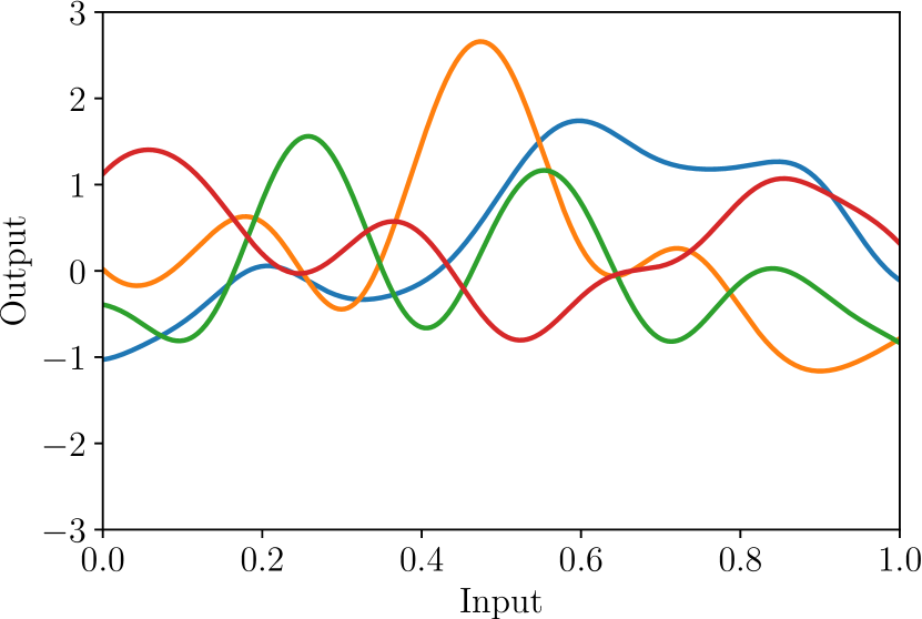
(a) $\mathcal{K}_{\mathrm{SE}}$

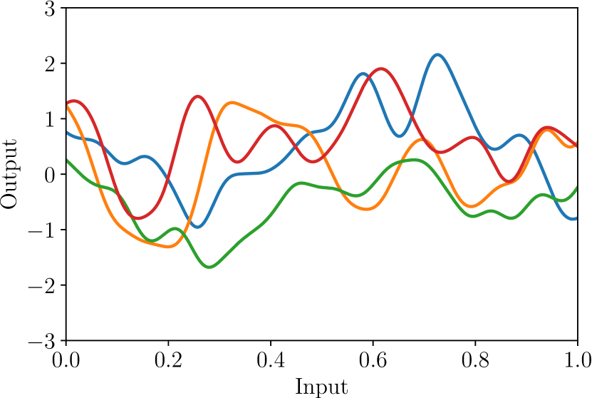
(b) $\mathcal{K}_{\mathrm{RQ}}$

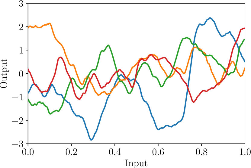
(c) $\mathcal{K}_{\mathrm{Matern32}}$

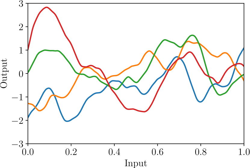
(d) $\mathcal{K}_{\mathrm{Matern52}}$

In Figures 2 and 3, we consider a training set of $7$ patterns measured without noise from the cardinal sine function $\mathop{\rm sinc}\left(2x\right)$ and we report the corresponding posterior distribution $\hat{f}\left(x^{\star}\right)$ for two different kernels. The blue solid line corresponds to the prediction, whereas the shaded area shows the $95\%$ confidence interval of the forecast. We notice that the square exponential kernel produces a lower interpolation variance (Figure 2) than the Matern32 kernel (Figure 3), whereas the extrapolation variance is similar for the two kernel functions.

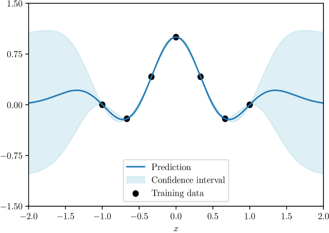
Figure 2: Posterior distribution of $\mathop{\rm sinc}\left(2x\right)$ ($\mathcal{K}_{\mathrm{SE}}$ kernel)

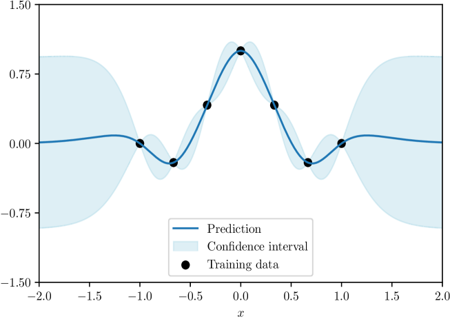
Figure 3: Posterior distribution of $\mathop{\rm sinc}\left(2x\right)$ ($\mathcal{K}_{\mathrm{Matern52}}$ kernel)

Periodic exponential kernel

When working with time series, it is useful to be able to include periodicity effects. Some covariance kernels exhibit this property, like the periodic exponential kernel (MacKay, 1998):

$$\mathcal{K}_{\mathrm{PE}}\left(x,x^{\prime}\right)=\sigma^{2}\exp\left(-\frac{1}{2}\sum_{j=1}^{d}\frac{1}{\ell_{j}^{2}}\sin^{2}\left(\frac{\pi}{\lambda_{j}}\left(x_{j}-x_{j}^{\prime}\right)\right)\right)$$

where each dimension of the input space has a period $\lambda_{j}$. More periodic kernels can be computed from other kernels, such as the Matérn class. They can actually be built from any kernel for which the Gram matrix on a periodic basis can be computed (Durrande, 2016).

Remark 4.

Since kernels can be combined in various ways, we will often be interested in separating time patterns from space patterns. If one observation is defined by the couple $\left(t,x\right)$ where $x\in\mathbb{R}^{d}$ and $t\in\mathbb{R}$ is the time index, we can then define a kernel on the whole space-time (Osborne et al., 2012):

$$\mathcal{K}\left(\left(x,t\right),\left(x^{\prime},t^{\prime}\right)\right)=\mathcal{K}_{\textrm{Time}}\left(t,t^{\prime}\right)\cdot\mathcal{K}_{\textrm{Space}}\left(x,x^{\prime}\right)$$

where $\mathcal{K}_{\textrm{Time}}$ is the kernel function for time patterns and $\mathcal{K}_{\textrm{Space}}$ is the kernel function for space patterns.

Spectral mixture kernel

Wilson and Adams (2013) introduce a new kernel construction method based on Gaussian mixtures in the Fourier space. For that, they use the Bochner’s theorem, which states that a real-valued function $k$ defined on $\mathbb{R}^{d}$ is a covariance kernel of a stationary continuous random process if and only if it can be represented in the following way:

$$k\left(s\right)=\int_{\mathbb{R}^{d}}e^{2\pi i\lambda^{\top}s}\,\mu\left(\mathrm{d}\lambda\right)$$

where $\mu$ is a positive finite measure on $\mathbb{R}^{d}$. This theorem establishes equivalence between stationary covariance kernels and their Fourier transform. It is a generalization of the classic one-dimensional spectral analysis when dealing with kernel functions instead of autocovariance functions. Indeed, the spectral density function $f_{k}\left(\lambda\right)$ is the Fourier transform of the covariance kernel function:

$$f_{k}\left(\lambda\right)=\int_{\mathbb{R}^{d}}k\left(s\right)e^{-2\pi i\lambda^{\top}s}\,\mathrm{d}s$$

whereas the covariance kernel function is the inverse Fourier transform of the spectral density function $f_{k}\left(\lambda\right)$:

$$k\left(s\right)=\int_{\mathbb{R}^{d}}f_{k}\left(\lambda\right)e^{2\pi i\lambda^{\top}s}\,\mathrm{d}\lambda$$

For instance, the SE kernel has a spectral density which is Gaussian. This leads Wilson and Adams (2013) to consider Gaussian mixtures of spectral densities to extend the SE kernel.

Let us define a mixture of $n_{m}$ Gaussian densities on $\mathbb{R}^{d}$ with mean vectors $\left(\mu_{1},\ldots,\mu_{n_{m}}\right)$ and diagonal covariance matrices $\left(\Sigma_{1},\ldots,\Sigma_{n_{m}}\right)$. The corresponding density function $g\left(x\right)$ is defined by:

$$g\left(x\right)=\sum_{m=1}^{n_{m}}\omega_{m}\frac{1}{\left({2\pi}\right)^{d/2}\sqrt{\mathop{\rm det}\Sigma_{m}}}\exp\left(-\left(x-\mu_{m}\right)^{\top}\Sigma_{m}^{-1}\left(x-\mu_{m}\right)\right)$$ (4)

where $\omega_{m}$ is the weight of the $m^{\mathrm{th}}$ Gaussian distribution. In our case, we are interested in real-valued covariance functions, implying that we replace $g\left(x\right)$ by $\frac{1}{2}\left(g\left(x\right)+g\left(-x\right)\right)$. Interestingly, the inverse Fourier transform of Equation (4) is analytically tractable and is given by:

$$k_{\mathrm{SM}}\left(s\right)=\sum_{m=1}^{n_{m}}\omega_{m}\cos\left(2\pi s^{\top}\mu_{m}\right)\exp\left(-2\pi^{2}s^{\top}\Sigma_{m}s\right)$$

Wilson and Adams (2013) show that the spectral mixture (SM) kernel can recover the usual kernels (squared exponential, Matérn, rational quadratic). Another interesting property is that it can learn negative covariances, which is essential when considering mean-reverting processes and contrarian trading strategies.

2.1.4 Hyperparameter selection

The covariance functions introduced before all have hyperparameters, such as length scales $\Sigma=\mathop{\rm diag}\left(\ell_{1}^{2},\ldots,\ell_{d}^{2}\right)$ in the squared exponential kernel, power $\alpha$ in the rational quadratic kernel, etc. All these parameters influence how the GP model can fit the observed data. This is why their choice is critical. They can be fixed ex-ante or we can estimate them.

For a given model, we denote by $\theta$ the parameters of the model. The usual way of selecting parameters is to maximize the likelihood function $L\left(\theta\right)=p\left(y\mid\theta\right)$. The underlying idea is to maximize the probability of the sample data $y$. In the case of the Gaussian process regression, $\theta=\left(\theta_{\mathcal{K}},\sigma_{\varepsilon}\right)$ consists of the parameters $\theta_{\mathcal{K}}$ of the kernel function and the standard deviation $\sigma_{\varepsilon}$ of the noise. Let $z=f\left(x\right)$ be the GP. We have:

$$p\left(y\mid\theta\right)=\int p\left(y\mid\theta,z\right)p\left(z\mid\theta\right)\,\mathrm{d}z$$

It is common to maximize the log marginal likelihood where we integrate out the latent values of $z$ and solve:

$$\hat{\theta}=\arg\max_{\theta}\boldsymbol{\ell}\left(\theta\right)$$

where $\boldsymbol{\ell}\left(\theta\right)=\ln p\left(y\mid\theta\right)$. In the case of Gaussian noise, we have $Y\sim\mathcal{N}\left(\mathbf{0}_{n},\mathcal{K}\left(\theta_{\mathcal{K}}\right)+\sigma_{\varepsilon}^{2}I_{n}\right)$ where $\mathcal{K}\left(\theta_{\mathcal{K}}\right)$ denotes the kernel matrix that depends on the kernel parameters $\theta_{\mathcal{K}}$. It follows that:

$$\boldsymbol{\ell}\left(\theta\right)=-\frac{n}{2}\ln\left(2\pi\right)-\frac{1}{2}\ln\left|\mathcal{K}\left(\theta_{\mathcal{K}}\right)+\sigma_{\varepsilon}^{2}I_{n}\right|-\frac{1}{2}Y^{\top}\left(\mathcal{K}\left(\theta_{\mathcal{K}}\right)+\sigma_{\varepsilon}^{2}I_{n}\right)^{-1}Y$$

This problem is usually solved using gradient-descent or quasi-Newton algorithms since it is possible to compute analytically the gradient of $\mathcal{K}\left(\theta_{\mathcal{K}}\right)$. However, $\boldsymbol{\ell}\left(\theta\right)$ is not always convex, and may suffer local maxima (Duvenaud, 2013).

Let us illustrate the ML estimation of the hyperparameters with the periodic kernel. For that, we use $7$ training points. In Figure 4, we report the posterior distribution $f\left(x^{\star}\mid x,y\right)$ when $x^{\star}$ ranges from $-3$ to $+3$. We assume that the hyperparameters of the kernel function are $\sigma=1$, $\lambda_{1}=2$ and $\ell_{1}=1$ whereas the standard deviation of the noise $\sigma_{\varepsilon}$ is set to $10^{-7}$. Then, we estimate the parameters $\theta=\left(\sigma,\lambda_{1},\ell_{1},\sigma_{\varepsilon}\right)$ by the method of maximum likelihood. We obtain $\hat{\sigma}=0.7657$, $\hat{\lambda}_{1}=1.6506$, $\hat{\ell}_{1}=0.7664$ and $\sigma_{\varepsilon}=2.46\times 10^{-7}$. The corresponding posterior distribution is given in Figure 5. As expected, we better fit the training set after the ML estimation than before.

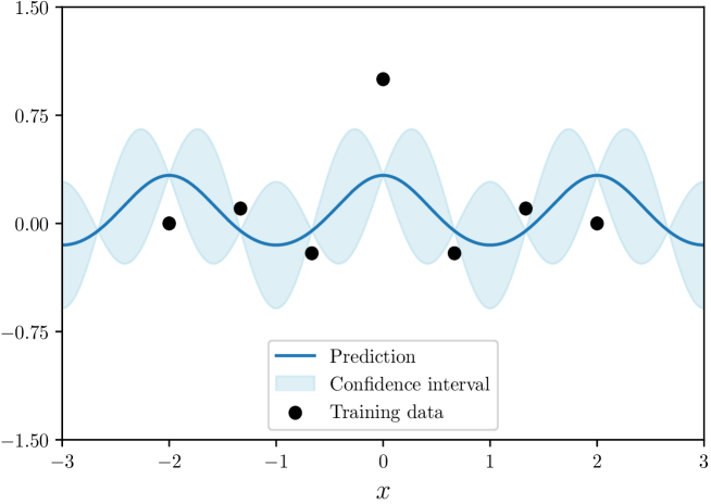
Figure 4: Posterior distribution before marginal likelihood maximization

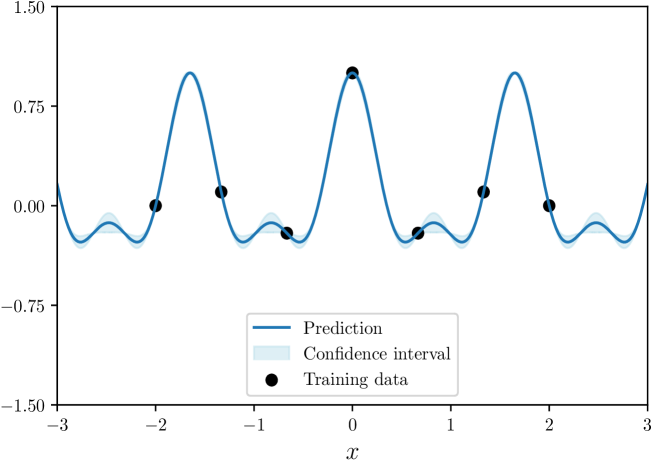
Figure 5: Posterior distribution after marginal likelihood maximization

Remark 5.

The Bayesian approach puts a prior distribution on the hyperparameters $\theta$ and marginalizes the posterior GP distribution over $\theta$. However, this is not analytically tractable. We also notice that the posterior distribution of the GP is intractable if the noise is non-Gaussian. Both cases require to use Monte Carlo methods such as the Hamiltonian or Hybrid Monte Carlo (Neal, 2011), which is described in Appendix A.4 on page A.4.

2.1.5 Classification

Gaussian processes regression can be extended for classification problems, where the output is a discrete variable corresponding to the class index. For example, we could want to predict the movements of asset prices: $1$ for a positive return and $0$ otherwise. In what follows, we consider the case of binary classification.

To model two classes with a GP prior over the data, one generally uses a sigmoid function $g\left(x\right)$, for example the logistic function $\mathop{\rm logit}\left(x\right)=\left(1+e^{-x}\right)^{-1}$. The output $y$ is such that:

$$\Pr\left\{y=1\right\}=g\left(f\left(x\right)\right)$$

where $f\left(x\right)$ is the GP over $\mathcal{X}$. The predictive distribution for new inputs $x^{\star}$ can be marginalized over the latent GP values:

$$p\left(z^{\star}\mid y,z\right)=\int p\left(z^{\star}\mid z\right)p\left(z\mid y\right)\,\mathrm{d}z$$

where $z$ and $z\mathbf{{}^{\star}}$ respectively denote the random variables $f\left(x\right)$ and $f\left(x^{\star}\right)$. We deduce that:

$$\Pr\left\{y^{\star}=1\mid y\right\}=\int g\left(z^{\star}\right)p\left(z^{\star}\mid z\right)p\left(z\mid y\right)\,\mathrm{d}z^{\star}\,\mathrm{d}z$$ (5)

where the posterior distribution $p\left(z\mid y\right)$ can be written using Bayes rule:

$$p\left(z\mid y\right)=\frac{p\left(y\mid z\right)p\left(z\right)}{p\left(y\right)}$$

Here, $p\left(z^{\star}\mid z\right)$ is the usual posterior distribution of the GP. However, the posterior distribution $p\left(z\mid y\right)$ is not easy to compute, and this is why approximations are used to evaluate the integral (5). Laplace approximation and expectation propagation are the two popular methods (Rasmussen and Williams, 2006). The first one approximates the posterior using a two-order Taylor expansion around its maximum, while the second one approximates the intractable probability distribution by minimizing the Kullback-Leibler divergence.

2.2 Bayesian optimization

Bayesian optimization is a black-box optimization method, meaning that little information is known about the objective function $f\left(x\right)$. Typically, Bayesian optimization is useful when the function is expensive to evaluate, its analytical expression is inaccessible or the gradient vector is not stable. This is the case with many complex machine learning problems where one would like to optimize the hyperparameters. For instance, the score of a deep neural network architecture is difficult to compute for a given set of hyperparameters (because training the model itself can take a long time), and it is impossible to compute the gradient vector with respect to each hyperparameter.

2.2.1 General principles

We are interested in finding the maximum of $f\left(x\right)$ on some bounded set $\mathcal{X}$. Bayesian optimization consists of two parts: (1) the ‘probabilistic surrogate’ and (2) the ‘acquisition function’ (or utility function). First of all, we build a prior probabilistic model for the objective function $f\left(x\right)$, and then update the probability distribution with samples drawn from $f\left(x\right)$ to get a posterior probability distribution. This approximation of the objective function is called a surrogate model. Gaussian processes are a popular surrogate model for Bayesian optimization because the GP posterior is still a multivariate normal distribution. We then use a utility function based on this posterior probability distribution to choose a new point to evaluate the objective function at the next step. This utility function is called acquisition function. Intuitively, we consider the trade-off between exploitation and exploration. Exploitation means sampling where the surrogate model predicts a high objective gain and exploration means sampling where the prediction uncertainty is high. Therefore, the general idea of Bayesian optimization consists of the following steps:

1. Place a GP prior on the objective function $f\left(x\right)$.

2. Update the GP posterior probability distribution on $f\left(x\right)$ with all available samples.

3. Based on the acquisition function, decide where to make the next measurement.

4. Given this measurement, update the GP posterior probability distribution.

5. Repeat steps 2-4 until an approximated maximum of the objective function $f\left(x\right)$ is obtained (or stop after a predefined number of iterations).

2.2.2 Acquisition function

We assume that the function $f\left(x\right)$ has a Gaussian process prior and we observe samples of the form $\left\{\left(x_{i},y_{i}\right)\right\}_{i=1}^{n}$. We have $y_{i}=f\left(x_{i}\right)+\varepsilon_{i}$ where $\varepsilon_{i}\sim\mathcal{N}\left(0,\sigma_{\varepsilon}^{2}\right)$ is the noise process. We denote by $x$ and $y$ the matrices $\left(x_{1},\dots,x_{n}\right)$ and $\left(y_{1},\dots,y_{n}\right)$. As shown previously, we can compute the posterior probability distribution $f\left(x^{\star}\mid x,y\right)$ for a new observation $x^{\star}$, and we have:

$$\hat{f}_{n}\left(x^{\star}\right)\sim\mathcal{N}\left(\hat{m}_{n}\left(x^{\star}\right),\mathcal{\hat{K}}_{n}\left(x^{\star},x^{\star}\right)\right)$$

where:

$$\hat{m}_{n}\left(x^{\star}\right)=\mathcal{K}\left(x^{\star},x\right)\left(\mathcal{K}\left(x,x\right)+\sigma_{\varepsilon}^{2}I_{n}\right)^{-1}y$$

and:

$$\mathcal{\hat{K}}_{n}\left(x^{\star},x^{\star}\right)=\mathcal{K}\left(x^{\star},x^{\star}\right)-\mathcal{K}\left(x^{\star},x\right)\left(\mathcal{K}\left(x,x\right)+\sigma_{\varepsilon}^{2}I_{n}\right)^{-1}\mathcal{K}\left(x,x^{\star}\right)$$

The subscript $n$ indicates that $\hat{f}_{n}$, $\hat{m}_{n}$ and $\mathcal{\hat{K}}_{n}$ depend on the sample of size $n$, which corresponds to the optimization step $n$. We note $\mathcal{D}_{n}$ the augmented data with the GP:

$$\mathcal{D}_{n}=\left\{\left(x_{i},y_{i},\hat{f}_{i}\left(x_{i}\right)\right)\right\}_{i=1}^{n}$$

Let $\mathcal{U}_{n}\left(x^{\star}\right)$ be the acquisition (or utility) function based on $\mathcal{D}_{n}$. The Bayesian optimization consists then in finding the new optimal point $x_{n+1}\in\mathcal{X}$ such that:

$$x_{n+1}=\arg\max\,\mathcal{U}_{n}\left(x^{\star}\right)$$

and updating the set of observations and the posterior distribution (see Algorithm 1).

Algorithm 1 Bayesian optimization algorithm

  The goal is to perform a Bayesian optimization

  We initialize the data sample $\mathcal{D}_{1}$ and the vector $\theta_{1}$ of hyperparameters

  for $n=1,2,\ldots$ do

     Find the optimal value $x_{n+1}\in\mathcal{X}$ of the utility maximization problem:

$$x_{n+1}=\arg\max\,\mathcal{U}_{n}\left(x^{\star}\right)$$

     Update the data:

$$\mathcal{D}_{n+1}\leftarrow\mathcal{D}_{n}\cup\left\{\left(x_{n+1},y_{n+1},\hat{f}_{n+1}\left(x_{n+1}\right)\right)\right\}$$

     Update the hyperparameter vector $\theta_{n+1}$ of the kernel function

  end for

  return  $\mathcal{D}_{n}$ and $\theta_{n}$

Improvement-based acquisition function

Let $f_{n}\left(\varkappa_{n}^{\star}\right)$ be the current optimal value among $n$ samples drawn from $f\left(x\right)$:

$$\varkappa_{n}^{\star}=\arg\max_{\varkappa\in x}f\left(\varkappa\right)$$

where $\varkappa_{n}^{\star}$ is the point that maximizes the GP function over the first $n$ steps. We would like to choose the next point $x_{n+1}$ to be evaluated in order to improve this value. We define the improvement $\Delta_{n}\left(x^{\star}\right)$ as follows:

$$\Delta_{n}\left(x^{\star}\right) = \left(\hat{f}_{n}\left(x^{\star}\right)-f_{n}\left(\varkappa_{n}^{\star}\right)\right)^{+}$$

$$= \max\left(\hat{f}_{n}\left(x^{\star}\right)-f_{n}\left(\varkappa_{n}^{\star}\right),0\right)$$

The most intuitive strategy, as proposed by Kushner (1964), is to choose the point that maximizes the probability of a positive improvement:

$$\Pr\left\{\Delta_{n}\left(x^{\star}\right)>0\right\} = \Pr\left\{\hat{f}_{n}\left(x^{\star}\right)>f_{n}\left(\varkappa_{n}^{\star}\right)\right\}$$

$$= \Pr\left\{\mathcal{N}\left(0,1\right)>\frac{f_{n}\left(\varkappa_{n}^{\star}\right)-\hat{m}_{n}\left(x^{\star}\right)}{\sqrt{\mathcal{\hat{K}}_{n}\left(x^{\star},x^{\star}\right)}}\right\}$$

$$= \Phi\left(\frac{\hat{m}_{n}\left(x^{\star}\right)-f_{n}\left(\varkappa_{n}^{\star}\right)}{\sqrt{\mathcal{\hat{K}}_{n}\left(x^{\star},x^{\star}\right)}}\right)$$

Since the probability of improvement fails to quantify the level of improvement, Močkus (1975) introduces an alternative acquisition function which takes into account the expected value of improvement (EI):

$$\mathop{\rm EI}\nolimits_{n}\left(x^{\star}\right)=\mathbb{E}\left[\Delta_{n}\left(x^{\star}\right)\right]$$

In the GP framework, we obtain a closed form of the expected improvement acquisition function:

$$\mathop{\rm EI}\nolimits_{n}\left(x^{\star}\right) = \left(\hat{m}_{n}\left(x^{\star}\right)-f_{n}\left(\varkappa_{n}^{\star}\right)\right)\Phi\left(\frac{\hat{m}_{n}\left(x^{\star}\right)-f_{n}\left(\varkappa_{n}^{\star}\right)}{\sqrt{\mathcal{\hat{K}}_{n}\left(x^{\star},x^{\star}\right)}}\right)+$$

$$\sqrt{\mathcal{\hat{K}}_{n}\left(x^{\star},x^{\star}\right)}\phi\left(\frac{\hat{m}_{n}\left(x^{\star}\right)-f_{n}\left(\varkappa_{n}^{\star}\right)}{\sqrt{\mathcal{\hat{K}}_{n}\left(x^{\star},x^{\star}\right)}}\right)$$

It follows that $\mathop{\rm EI}_{n}\left(x^{\star}\right)$ and its derivatives are easy to evaluate, and we can use optimization algorithms such as quasi-Newton methods to find its maximum. Here, we have defined two utility functions $\mathcal{U}_{n}\left(x^{\star}\right)=\Pr\left\{\Delta_{n}\left(x^{\star}\right)>0\right\}$ and $\mathcal{U}_{n}\left(x^{\star}\right)=\mathop{\rm EI}_{n}\left(x^{\star}\right)$ that are good candidates of acquisition functions. Applications of improvement-based acquisition functions are studied in Jones et al. (1998), Jones (2001), Brochu et al. (2010), and Shahriari et al. (2016), whereas the convergence of improvement-based optimization has been shown by Bull (2011). Appendix A.6 on page A.6 extends the previous results to minimization problems.

Remark 6.

The previous approach can be generalized by considering a given threshold $\tau$. In this case, we define the improvement by $\Delta_{n}\left(x^{\star}\right)=\left(\hat{f}_{n}\left(x^{\star}\right)-\tau\right)^{+}$. We have:

$$\Pr\left\{\Delta_{n}\left(x^{\star}\right)>0\right\}=\Phi\left(\frac{\hat{m}_{n}\left(x^{\star}\right)-\tau}{\sqrt{\mathcal{\hat{K}}_{n}\left(x^{\star},x^{\star}\right)}}\right)$$

and:

$$\mathop{\rm EI}\nolimits_{n}\left(x^{\star}\right)=\left(\hat{m}_{n}\left(x^{\star}\right)-\tau\right)\Phi\left(\frac{\hat{m}_{n}\left(x^{\star}\right)-\tau}{\sqrt{\mathcal{\hat{K}}_{n}\left(x^{\star},x^{\star}\right)}}\right)+\sqrt{\mathcal{\hat{K}}_{n}\left(x^{\star},x^{\star}\right)}\phi\left(\frac{\hat{m}_{n}\left(x^{\star}\right)-\tau}{\sqrt{\mathcal{\hat{K}}_{n}\left(x^{\star},x^{\star}\right)}}\right)$$

Most of the time, the threshold $\tau$ is set to $f_{n}\left(\varkappa_{n}^{\star}\right)+\xi$ where $\xi>0$.

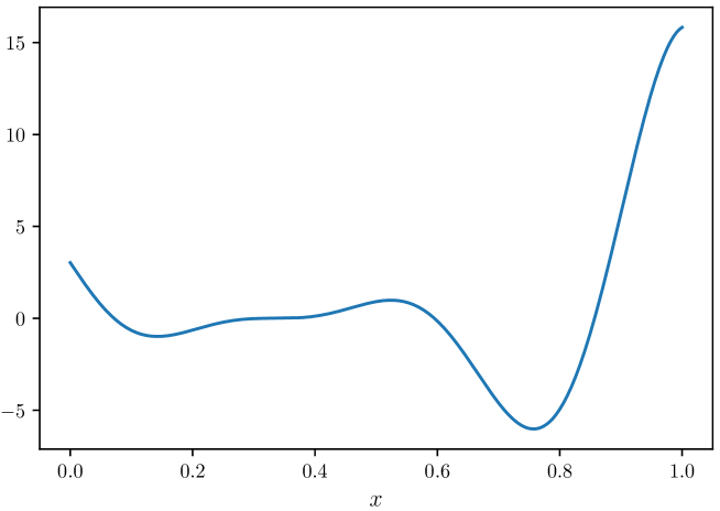
Figure 6: Objective function of the minimization problem

In Figure 7, we illustrate the improvement-based optimization using the following minimization problem:

$$\min f\left(x\right)=\left(6x-2\right)^{2}\sin\left(12x-4\right)$$

The objective function $f\left(x\right)$ is reported in Figure 6. In practice, we start with an initial design, usually consisting in measuring several random points of the domain. In the top/left panel in Figure 7, we start the algorithm with three initial points. We report the mean (blue solid line) and the confidence interval (blue shaded area) of the GP distribution. We also show the acquisition function $\mathcal{U}_{n}\left(x^{\star}\right)=\mathop{\rm EI}\nolimits_{n}\left(x^{\star}\right)$ (red dashed line) and indicate the suggested next location by a vertical black line, which corresponds to the maximum of $\mathcal{U}_{n}\left(x^{\star}\right)$. The top/right panel corresponds to the second iteration where we have updated the sample. Indeed, the sample now contains the initial three points and the maximum point $x^{\star}$ obtained at the previous iteration. Then, we continue the process and show the results of the Bayesian optimization for the next five steps. We notice that steps $n=3$, $n=4$ and $n=5$ correspond to an exploration stage (sampling where the variance is high), whereas step $n=1$, $n=2$ and $n=6$ corresponds to an exploitation stage (sampling where the improvement is high). Finally, after six iterations, we have located the minimum since the acquisition function is equal to zero.

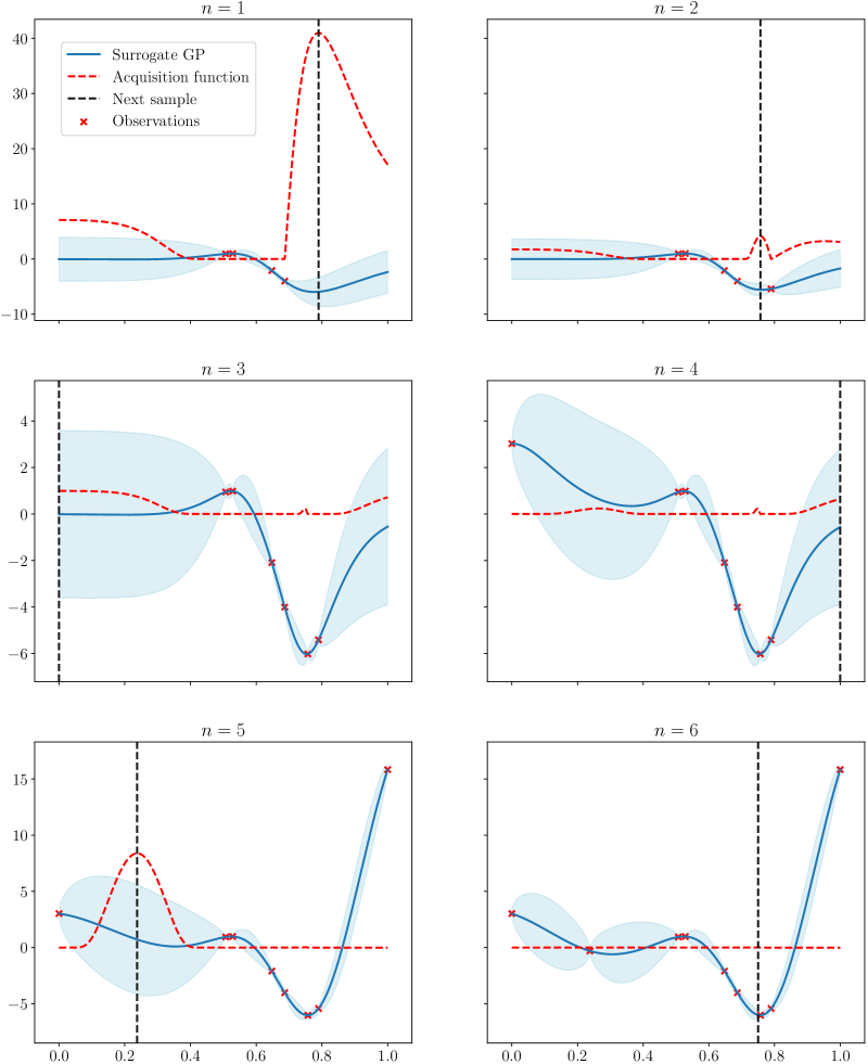
Figure 7: Iterations of the Bayesian optimization

Entropy-based acquisition function

In this paragraph, we introduce two other acquisition functions based on differential entropy of information theory. Given random variables $X$ and $Y$ with continuous probability functions $p\left(x\right)$ and $p\left(y\right)$ and joint probability function $p\left(x,y\right)$, the differential (or Shannon) entropy $H\left(X\right)$ is equal to:

$$H\left(X\right)=-\int p\left(x\right)\ln p\left(x\right)\,\mathrm{d}x$$

while the conditional differential entropy $H\left(X\mid Y\right)$ of $X$ is defined by:

$$H\left(X\mid Y\right)=-\int\int p\left(x,y\right)\ln p\left(x\mid y\right)\,\mathrm{d}x\,\mathrm{d}y$$

Using Bayes theorem, we note that $H\left(X\mid Y\right)$ is the result of averaging $H\left(X\mid Y=y\right)$ over all possible values $y$ of the random variable $Y$ (Cover and Thomas, 2012).

We consider the location $x_{\max}$ of the global maximum of $f\left(x\right)$ as a random variable, which has the posterior distribution $\hat{p}_{n}\left(x_{\max}\right)=p\left(x_{\max}\mid x,y\right)$. Then, we can use the differential entropy to quantify the uncertainty of this point. The smaller the differential entropy, the lower the uncertainty. In order to have more certainty about the location of the global minimum, we want to choose the next point to evaluate $x_{n+1}$ that implies the largest decrease in the differential entropy. For this purpose, we define the entropy search (ES) acquisition function as the difference between the current differential entropy of $\hat{p}_{n}\left(x_{\max}\right)$ and the expected differential entropy of posterior probability distribution $p\left(x_{\max}\mid x,y,x^{\star},\hat{f}_{n}\left(x^{\star}\right)\right)$ after adding a new sample $\left\{x^{\star},\hat{f}_{n}\left(x^{\star}\right)\right\}$:

$$\mathop{\rm ES}\nolimits_{n}\left(x^{\star}\right)=H\left(x_{\max}\right)-H\left(x_{\max}\mid\hat{f}_{n}\left(x^{\star}\right)\right)$$

It follows that the next point is the solution of the maximization problem:

$$x_{n+1}=\arg\max_{x^{\star}\in\mathcal{X}}\mathop{\rm ES}\nolimits_{n}\left(x^{\star}\right)$$

Although Henning and Schuler (2012) propose a method to approximate the above equation, Frazier (2018) indicates some difficulties in practice:

• $\hat{p}_{n}\left(x_{\max}\right)$ does not have always a closed-form expression;

• we need to compute the differential entropy of a large number of samples of $\left\{x^{\star},\hat{f}_{n}\left(x^{\star}\right)\right\}$ to evaluate the expectation in the second term $H\left(x_{\max}\mid\hat{f}_{n}\left(x^{\star}\right)\right)$.

This is why Hernández-Lobato et al. (2014) propose an alternative approach called predictive entropy search (PES):

$$\mathop{\rm PES}\nolimits_{n}\left(x^{\star}\right)=H\left(\hat{f}_{n}\left(x^{\star}\right)\right)-H\left(\hat{f}_{n}\left(x^{\star}\right)\mid x_{\max}\right)$$

Using the symmetric property of the mutual information, we can demonstrate that $\mathop{\rm PES}\nolimits_{n}\left(x^{\star}\right)$ and $\mathop{\rm ES}\nolimits_{n}\left(x^{\star}\right)$ are equivalent acquisition functions. In the case of the PES acquisition function, we can compute a closed-form expression for $H\left(\hat{f}_{n}\left(x^{\star}\right)\right)$ and Hernández-Lobato et al. (2014) uses the expectation propagation method (Minka, 2001) to find an approximation of $H\left(\hat{f}_{n}\left(x^{\star}\right)\mid x_{\max}\right)$. Therefore, we can find the maximum of the PES acquisition function by a simulation approach.

Knowledge gradient-based acquisition function

The knowledge gradient (KG) acquisition function is closed to the expected improvement. It was first introduced in Frazier et al. (2009) for finite discrete decision spaces before Scott et al. (2011) extended it to Gaussian processes. The main difference between KG and EI acquisition functions is that KG accounts for noise and does not restrict the final solution to a previously evaluated point, meaning that it can return any point of the domain and not only one observed point.

Suppose that we have observed the sample $\left\{\left(x_{i},y_{i}\right)\right\}_{i=1}^{n}$. As previously, we compute the posterior probability distribution:

$$\hat{f}_{n}\left(x^{\star}\right)\sim\mathcal{N}\left(\hat{m}_{n}\left(x^{\star}\right),\mathcal{\hat{K}}_{n}\left(x^{\star},x^{\star}\right)\right)$$

Under risk-neutrality assumption (Berger, 2013), we value a random outcome according to its expected value $\hat{m}_{n}\left(x^{\star}\right)$. To maximize the objective function, we can try to maximize $\hat{m}_{n}\left(x^{\star}\right)$ and we note $\hat{m}_{n}\left(\varkappa_{n}^{\star}\right)=\max_{\varkappa}\hat{m}_{n}\left(\varkappa\right)$. If we consider one supplementary point, we could also compute the new posterior distribution for $f$ with conditional expected value $\hat{m}_{n+1}\left(x^{\star}\right)$. The idea is then to choose a new point that maximizes the increment in conditioned expectation gained from sampling this point. For example, we can maximize the expected value of the difference, which is called knowledge gradient:

$$\mathop{\rm KG}\nolimits_{n}\left(x^{\star}\right)=\mathbb{E}\left[\hat{m}_{n+1}\left(x^{\star}\right)-\hat{m}_{n}\left(\varkappa_{n}^{\star}\right)\right]$$

We have:

$$x_{n+1}=\arg\max_{x^{\star}\in\mathcal{X}}\mathop{\rm KG}\nolimits_{n}\left(x^{\star}\right)$$

The solution can then be obtained via simulation using Algorithm 2 formulated by Frazier (2018).

Algorithm 2 Simulation-based computation of $\mathop{\rm KG}\nolimits_{n}\left(x^{\star}\right)$

  $x^{\star}$ is the input parameter

  $n_{s}$ is the number of simulations

  We note $\hat{m}_{n}\left(\varkappa_{n}^{\star}\right)=\max_{\varkappa}\hat{m}_{n}\left(\varkappa\right)$

  for $s=1:n_{s}$ do

     Generate $y_{\left(s\right)}^{\star}\sim\mathcal{N}\left(\hat{m}_{n}\left(x^{\star}\right),\mathcal{\hat{K}}_{n}\left(x^{\star},x^{\star}\right)\right)$

     Add the simulated point $(x^{\star},y_{\left(s\right)}^{\star})$ to the current sample $\left(x,y\right)$

     Compute $\hat{m}_{n+1}\left(\varkappa_{\left(s\right)}\right)=\max_{\varkappa\in\mathcal{X}}\hat{m}_{n+1}\left(\varkappa\right)$ where $\hat{m}_{n+1}\left(\varkappa\right)$ is the posterior mean that depends on $(x^{\star},y_{\left(s\right)}^{\star})$

     $\Delta_{\left(s\right)}\longleftarrow\hat{m}_{n+1}\left(\varkappa_{\left(s\right)}\right)-\hat{m}_{n}\left(\varkappa_{n}^{\star}\right)$

  end for

  return  $\mathop{\rm KG}\nolimits_{n}\left(x^{\star}\right)\leftarrow n_{s}^{-1}\sum_{s=1}^{n_{s}}\Delta_{\left(s\right)}$

Remark 7.

In the noise-free case and if the final solution is limited to the previous sampling, the KG acquisition function reduces to the EI acquisition function:

$$\hat{m}_{n+1}\left(x^{\star}\right)-\hat{m}_{n}\left(\varkappa^{\star}\right) = \max\left(f_{n}\left(\varkappa_{n}^{\star}\right),\hat{f}_{n}\left(x^{\star}\right)\right)-f_{n}\left(\varkappa_{n}^{\star}\right)$$

$$= \left(\hat{f}_{n}\left(x^{\star}\right)-f_{n}\left(\varkappa_{n}^{\star}\right)\right)^{+}$$

3 Financial applications

In this section, we use Gaussian processes to model and forecast the yield curve and Bayesian optimization to build an online trend-following strategy.

3.1 Yield curve modeling

To illustrate the potential of GP methods in finance, we first consider the fitting of the U.S. yield curve. One of the most used models is the Nelson-Siegel parametric model, for which problems have been reported regarding parameter estimation and their large variations over time (Annaert et al., 2013). GP can be thought of as a Bayesian nonparametric alternative. We display in Figures 8 and 9 the fitting of the yield curve corresponding to two different dates and presenting different shapes.

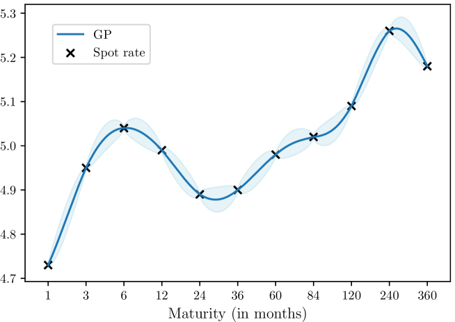
Figure 8: GP fitting of the yield curve (June 2007)

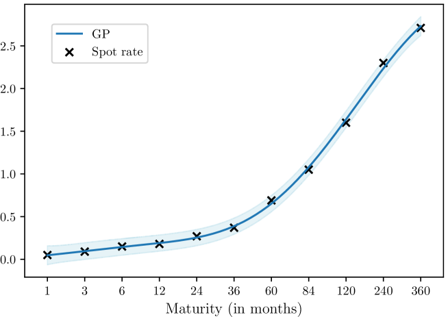
Figure 9: GP fitting of the yield curve (June 2012)

We now try GP-based methods to forecast movements of the U.S. yield curve. It is a classical macroeconomic factor that can be used as a signal in the forecasting of equity and bond returns (Rebonato, 2015; Cochrane et al. (2005)) and thus is of practical interest in quantitative asset management. Several approaches exist in time-series prediction with Gaussian processes. In this paper, we mainly focus on the GP-ARX model, which is an application of ARX models in the GP framework. The ARX model assumes a nonlinear relationship between the time-series $Y_{t}$ and its previous values plus some exogenous factors $X_{t}$:

$$Y_{t}=f\left(Y_{t-1},Y_{t-2},\dots,X_{t-1},X_{t-2},\dots\right)+\varepsilon_{t}$$

where $\varepsilon_{t}\sim\mathcal{N}\left(0,\sigma_{\varepsilon}^{2}\right)$ is a white noise process. The main idea of GP-ARX is to use a Gaussian process surrogate for the function $f\sim\mathcal{GP}\left(\mathbf{0},\mathcal{K}\right)$. Once the kernel $\mathcal{K}$ is chosen, the training set simply consists in observations of $X_{t}$ and $Y_{t}$. Inference of hyperparameters is done with the method of maximum likelihood as explained in the previous section. Chandorkar et al. (2017) use this model to forecast weather data and note the importance of the “persistence prediction” in model building. Persistence prediction is taking the current value as a forecast for tomorrow: $\hat{Y}_{t+1}=Y_{t}$. The persistence model assumes then that the process is a random walk. For time-series which exhibit memory effects, this trivial forecast yields very good results if we use usual accuracy measures, such as mean squared error. One way to measure memory in time-series is to compute the Hurst exponent, which measures the long-term autocorrelation. A Hurst exponent $H>\frac{1}{2}$ indicates positive long-term autocorrelation while $H<\frac{1}{2}$ is the opposite. The Hurst exponent is related to the fractal dimension of the time-series, and can be an indicator of the predictability of the time-series (Kroha and Škoula, 2018).

Table 1: Hurst exponent of U.S. spot rates

Maturity	1M	3M	6M	1Y	2Y	5Y	10Y	20Y	30Y
Hurst	$0.40$	$0.50$	$0.61$	$0.62$	$0.57$	$0.51$	$0.49$	$0.48$	$0.50$

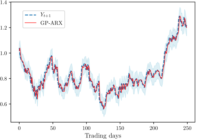
Figure 10: Prediction of the 2-year spot rate

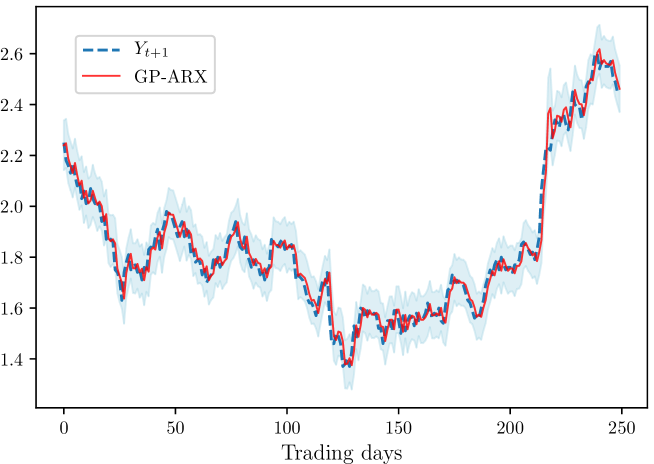
Figure 11: Prediction of the 10-year spot rate

Our dataset consists in daily zero-coupon yield for the following maturities: 1, 3 and 6 months, 1, 2, 5, 10, 20 and 30 years. Table 1 shows the Hurst exponent for the spot rates of different maturities. In Figures 10 and 11, we report the one-day ahead rolling prediction during 2016, and the $95\%$ confidence interval. We also forecast the 2Y and 10Y spot rates by using for each maturity a lag of one for the GP-ARX model, and the three-month spot rate and its first lag for the exogenous variable. Both spot rates exhibit persistence as it can be seen in Table 2. We notice that the three methods are equivalent in this simplistic example. However, the GP-ARX method is able to estimate the confidence interval, and this metric can be used as a trading signal.

Table 2: Root mean squared error (in %)

Spot Rate	Persistence	ARX	GP-ARX
2Y	$3.33$	$3.33$	$\mathbf{3.32}$
10Y	$\mathbf{4.40}$	$4.53$	$4.45$

Remark 8.

The choice of the kernel function and the features are primordial. The ARX model is actually equivalent to the GP-ARX model, when the kernel is linear. In our GP-ARX model, we used a sum of exponential and linear kernels and only used simple time-series features. Thanks to the ability to capture different length scales and patterns with the choice of the kernel, the GP approach can be used as good interpolators for a wide range of financial applications by finding the suitable kernel combination.

There is a growing interest in using Student-$t$ distribution instead of Gaussian distribution in GP regression (Shah et al., 2014). More specifically, Chen et al. (2014) introduce a framework for multivariate Gaussian and Student-$t$ process regression, and use it for stock and equity index predictions. The problem of yield curve forecasting is intrinsically multivariate. We are trying to predict a vector of interest rates for different maturities, that are highly correlated and dependent. Instead of treating each output separately, Student-$t$ multivariate process regression works with a dataset consisting of full yield curve observations as inputs and outputs at the same time, while taking into account output correlations. We recall in Appendix A.7 on page A.7 the definition and some useful properties of multivariate and matrix-variate Student-$t$ distributions. Specifically, as for the Gaussian case, the posterior distribution is still a matrix-variate Student-$t$ distribution, which makes computations of inference step and maximum marginal likelihood tractable. This motivates the definition of the Student-$t$ processes (TP). A collection of random vectors is a TP if and only if any finite number of them has a joint multivariate Student-$t$ distribution. We have tested TP-ARX in place of GP-ARX. Unfortunately, we have not found better forecasting values. This result is disappointing since we may think that one of the issues in yield curve modeling is the cross-section correlation of spot rates and the possible fat tails that we observe in fixed-income assets.

3.2 Portfolio optimization

We now consider an application of Bayesian optimization to portfolio optimization in the context of quantitative asset management. We first describe the asset allocation problem, which is a trend-following strategy, then we show how to solve it and finally we use Bayesian optimization with a squared exponential kernel to find optimal hyperparameters of the trend-following strategy.

3.2.1 The trend-following strategy

We consider a universe of $n$ assets for which we observe daily prices and we look for an optimal portfolio, that is an allocation vector $x\in\mathbb{R}^{n}$ that balances risk and return. If we can predict the vector $\mu$ of expected returns and compute the covariance matrix $\Sigma$ of asset returns, then the regularized Markowitz optimization problem (Roncalli, 2013; Bourgeron et al., 2018) is the following:

$$x^{\star}\left(\gamma\right)=\arg\min_{x}\frac{1}{2}x^{\top}\Sigma x-\gamma\mu^{\top}x+\lambda\left\|x-x_{0}\right\|_{2}^{2}$$

where $\gamma$ is the inverse of the risk-aversion coefficient, $\lambda$ is the ridge regularization parameter and $x_{0}$ is a reference portfolio. We consider a simple version of the trend-following strategy:

• The expected returns are computed using a moving-average estimator. Let $P_{i,t}$ be the daily price of Asset $i$. We have:

  $$\mu_{i,t}=\frac{P_{i,t}}{P_{i,t-\ell\left(\mu\right)}}-1$$

  where $\ell\left(\mu\right)$ is the window length of the MA estimator.

• The covariance matrix is estimated using the empirical estimator, the window length of which is denoted by $\ell\left(\Sigma\right)$.

• The portfolio is rebalanced at fixed dates $t$, for example on a monthly or weekly basis.

Let $x_{t}$ be the optimal portfolio at the rebalancing date $t$. The allocation problem is given by:

$$x_{t}\left(\lambda\right) = \arg\min_{x}-\mu_{t}^{\top}x+\lambda\left\|x-x_{t-1}\right\|_{2}^{2}$$

s.t. $$\sigma_{t}\left(x\right)\leq\bar{\sigma}$$

where $\mu_{t}$ is the estimated vector of expected returns at time $t$, $\sigma_{t}\left(x\right)=\sqrt{x^{\top}\Sigma_{t}x}$ is the portfolio volatility estimated at time $t$, $\bar{\sigma}$ is the target volatility of the trend-following strategy. To solve this convex problem, we use the ADMM algorithm given in Appendix A.8 on page A.8 (Boyd et al., 2011). Following Bourgeron et al. (2018) and Richard and Roncalli (2019), it is natural to write the previous problem as follows:

$$x_{t} = \arg\min_{x}-\mu_{t}^{\top}x+\lambda\left\|x-x_{t-1}\right\|_{2}^{2}+\mathds{1}_{\Omega}\left(z\right)$$

s.t. $$x-z=0$$

where $\Omega=\left\{z\in\mathbb{R}^{n}:\left\|z^{\top}\Sigma_{t}z\right\|_{2}^{2}\leq\bar{\sigma}^{2}\right\}$. However, we improve the ADMM algorithm by introducing the Cholesky trick:

$$x_{t} = \arg\min_{x}-\mu_{t}^{\top}x+\lambda\left\|x-x_{t-1}\right\|_{2}^{2}+\mathds{1}_{\Omega}\left(z\right)$$

s.t. $$-L_{t}x+z=0$$

where $\Omega=\left\{z\in\mathbb{R}^{n}:\left\|z\right\|_{2}^{2}\leq\bar{\sigma}^{2}\right\}$ and $L_{t}$ is the upper Cholesky decomposition matrix of $\Sigma_{t}$. It follows that $z=L_{t}x$ and:

$$\left\|z\right\|_{2}^{2} = z^{\top}z$$

$$= x^{\top}L_{t}^{\top}L_{t}x$$

$$= x^{\top}\Sigma_{t}x$$

$$= \sigma_{t}^{2}\left(x\right)$$

In fact, our experience shows that the Cholesky trick helps to accelerate the convergence of the ADMM algorithm with respect to the formulation of Bourgeron et al. (2018) and Richard and Roncalli (2019). Finally, it follows that the ADMM algorithm becomes:

$$x^{(k+1)} = \arg\min-\mu_{t}^{\top}x+\lambda\left\|x-x_{t-1}\right\|_{2}^{2}+\frac{\varphi}{2}\left\|-L_{t}x+z^{(k)}+u^{(k)}\right\|_{2}^{2}$$

$$z^{(k+1)} = \arg\min\mathds{1}_{\Omega}\left(z\right)+\frac{\varphi}{2}\left\|-L_{t}x^{(k+1)}+z+u^{(k)}\right\|_{2}^{2}$$

$$u^{(k+1)} = u^{(k)}-L_{t}x^{(k+1)}+z^{(k+1)}$$

We notice that the $z$-step corresponds to a simple projection on the Euclidean ball of center $0$ and radius $\bar{\sigma}$ of the vector $L_{t}x^{(k+1)}-u^{(k)}$, and the computation of the proximal operator is straightforward. The $x$-step corresponds to a linear system. If we define $f^{\left(k\right)}\left(x\right)$ as follows:

$$f^{\left(k\right)}\left(x\right)=-\mu_{t}^{\top}x+\lambda\left\|x-x_{t-1}\right\|_{2}^{2}+\frac{\varphi}{2}\left\|-L_{t}x+z^{(k)}+u^{(k)}\right\|_{2}^{2}$$

we deduce that:

$$\nabla f^{\left(k\right)}\left(x\right) = -\mu_{t}+\lambda x-\lambda x_{t-1}+\varphi L_{t}^{\top}L_{t}x-\varphi L_{t}^{\top}\left(z^{(k)}+u^{(k)}\right)$$

$$= -\mu_{t}+\lambda x-\lambda x_{t-1}+\varphi\Sigma_{t}x-\varphi L_{t}^{\top}\left(z^{(k)}+u^{(k)}\right)$$

Finally, we obtain the following solution:

$$x^{(k+1)}=\left(\varphi\Sigma_{t}+\lambda I_{n}\right)^{-1}\left(\mu_{t}+\lambda x_{t-1}+\varphi L_{t}^{\top}\left(z^{(k)}+u^{(k)}\right)\right)$$

3.2.2 Hyperparameter estimation of the trend-following strategy

The trend-following strategy depends on three hyperparameters:

1. the parameter $\lambda$ that controls the turnover between two rebalancing dates;

2. the window length $\ell\left(\mu\right)$ that controls the estimation of trends;

3. the horizon time $\ell\left(\Sigma\right)$ that measures the risk of the assets.

Traditionally, the trend-following strategy is implemented by considering that these hyperparameters are fixed. By construction, their choice has a big impact on the strategy design. For instance, a small value of $\ell\left(\mu\right)$ will catch short momentum, whereas a large value of $\ell\left(\mu\right)$ will look for more persistent trends. This hyperparameter is then key for distinguishing short-term and long-term CTAs.

In fact, the right asset allocation problem is not given by Equation (3.2.1), but is defined as follows:

$$x_{t}\left(\lambda_{t},\ell_{t}\left(\mu\right),\ell_{t}\left(\Sigma\right)\right) = \arg\min_{x}-\mu_{t}^{\top}x+\lambda_{t}\left\|x-x_{t-1}\right\|_{2}^{2}$$

s.t. $$\sigma_{t}\left(x\right)\leq\bar{\sigma}$$

This means that the hyperparameters are not fixed and must be estimated at each rebalancing date. In the previous framework, the estimation consists in finding $x_{t}$ given that $\lambda$, $\ell\left(\mu\right)$ and $\ell\left(\Sigma\right)$ are constant. In our framework, the estimation consists in finding the optimal portfolio $x_{t}$, but also the optimal parameters $\lambda_{t}$, $\ell_{t}\left(\mu\right)$ and $\ell_{t}\left(\Sigma\right)$. This can be done using the Bayesian optimization framework.

By nature, the parameters $\ell\left(\mu\right)$ and $\ell\left(\Sigma\right)$ are discrete and generally expressed in months, e.g. $\ell\left(\mu\right)\in\left\{3,6,12,24\right\}$ and $\ell\left(\Sigma\right)\in\left\{3,6,12\right\}$. Discrete, integer or categorical parameters are not easy to manage in Bayesian optimization since Gaussian processes (or random forests), which serve as surrogates for the black-box function, are not adapted. Since no standard approach exists yet, we use a simple method which consists in using continuous variables in the Bayesian optimization step while flooring the hyperparameters $\ell\left(\mu\right)$ and $\ell\left(\Sigma\right)$ to the nearest integer when computing the objective function given by Equation (3.2.2).

The choice of the objective function is the main step when implementing Bayesian optimization. In a classical machine learning problem, the objective function can be the cross-validation score of the hyperparameters, in order to reduce the risk of overfitting. Defining an objective for a quantitative strategy is less clear and prone to overfitting. One simple and obvious function is the Sharpe ratio of the strategy. Each rebalancing date, we run a Bayesian optimization to look for hyperparameters which maximizes the historical Sharpe ratio over a given period. A more robust objective function is the minimum of the rolling Sharpe ratio in order to reduce the overfitting bias. For example, we can compute the rolling six-month Sharpe ratio $\mathop{\rm SR}_{\tau}\left(\lambda,\ell\left(\mu\right),\ell\left(\Sigma\right)\right)$ for a backtest with fixed hyperparameters and a period $\left[\tau-0.5;\tau\right]$ and use Bayesian optimization to solve:

$$\left\{\lambda_{t},\ell_{t}\left(\mu\right),\ell_{t}\left(\Sigma\right)\right\}=\arg\max\left\{\min_{\tau\in\left[t-2,t\right[}\mathop{\rm SR}\nolimits_{\tau}\left(\lambda,\ell\left(\mu\right),\ell\left(\Sigma\right)\right)\right\}$$

However, in order to benefit from the exploration of the parameters space by Bayesian optimization, we use another approach. Since volatility is already controlled via the portfolio optimization constraint and regularization, we prefer to choose the return of the strategy over a two-year historical period for the objective function:

$$\left\{\lambda_{t},\ell_{t}\left(\mu\right),\ell_{t}\left(\Sigma\right)\right\}=\arg\max\hat{\mu}_{t}\left(\lambda,\ell\left(\mu\right),\ell\left(\Sigma\right)\right)$$

where $\hat{\mu}_{t}\left(\lambda,\ell\left(\mu\right),\ell\left(\Sigma\right)\right)$ is the performance of the backtest for the period $\left[t-2;t\right]$. We keep track of all samples tested during Bayesian optimization, sort them according to their objective function and select the best three sets of hyperparameters to compute three different optimal weights that are averaged to form the final portfolio. This approach considerably reduces the overfitting bias.

3.2.3 An example

Our dataset consists of daily prices of 13 futures contracts on world-wide equity indices such as the S&P 500 and Eurostoxx indices and 10Y sovereign bonds from 2006 to 2017. The Bayesian optimization strategy described in the previous paragraph is compared to the basic one-year trend-following strategy where parameters remain unchanged through time: $\lambda_{t}$ is set to $10\%$ while $\ell_{t}\left(\mu\right)$ and $\ell_{t}\left(\Sigma\right)$ are equal to $12$ months.

Table 3: Backtest results (2006 – 2016)

Strategy	Sharpe ratio	Return	Volatility	MDD
Naive	$1.56$	$5.9\%$	$3.7\%$	-$5.7\%$
Bayesian	$1.71$	$7.4\%$	$4.3\%$	-$4.7\%$

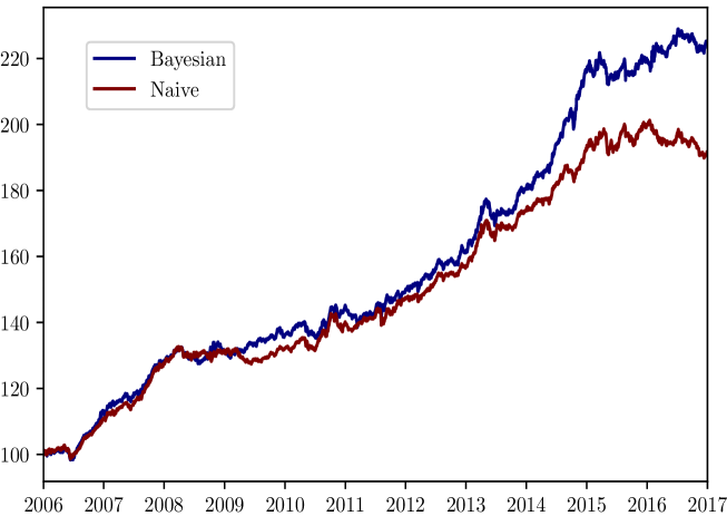
Figure 12: Cumulative performance of trend-following strategies

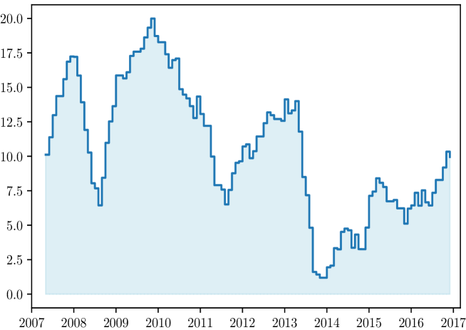
Figure 14: Estimated ridge penalization $\lambda_{t}$ (in %)

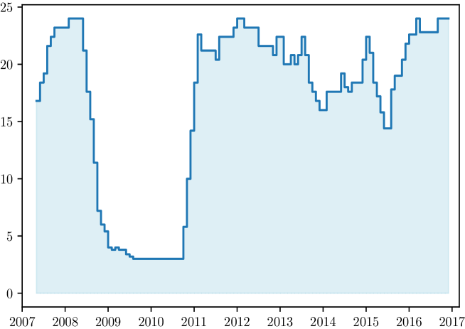
Figure 15: Estimated return window length $\ell_{t}\left(\mu\right)$ (in months)

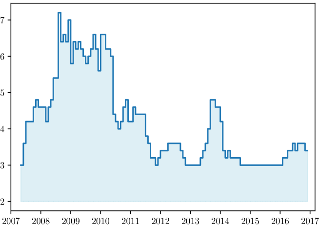
Figure 16: Estimated covariance window length $\ell_{t}\left(\Sigma\right)$ (in months)

The cumulative performance of the strategies is shown in Figure 12, whereas Table 3 shows the results of the two strategies. We notice that Bayesian optimization is able to improve the annualized Sharpe ratio from $1.56$ to $1.71$ and reduce drawdowns. However, we do not believe that this result is important, because it is just a backtest. More interesting are the dynamics of the hyperparameters estimated by the Bayesian optimization. On page 14, we report the dynamics of $\lambda_{t}$ (Figure 14), $\ell_{t}\left(\mu\right)$ (Figure 15) and $\ell_{t}\left(\Sigma\right)$ (Figure 16), whereas the statistics are reported in Table 4. We observe that $\lambda_{t}$ moves relatively fast. At the beginning of the 2008 Global Financial Crisis, it is reduced implying a more reactive allocation. At the end of the 2008 crisis, we observe the opposite effect. $\lambda_{t}$ is increased and the allocation becomes less reactive. However, this must be compared with the dynamics of $\ell_{t}\left(\mu\right)$ and $\ell_{t}\left(\Sigma\right)$. Most of the time, the optimal window $\ell_{t}\left(\mu\right)$ is high and is equal to 18 months on average. However, during and after the GFC, $\ell_{t}\left(\mu\right)$ is dramatically reduced. The parallel can be done with the performance of short-term and long-term CTAs. On average, long-term CTAs outperform short-term CTAs, but during some periods, short-term CTAs can do a very good job, and post an incredible performance while long-term CTAs have a strong negative performance. Concerning $\ell_{t}\left(\Sigma\right)$, the results indicate that a short-term window is better, while the market practice is to consider long-term window (typically a one-year empirical covariance matrix). In fact, there is a trade-off between the regularization parameter $\lambda_{t}$ and the covariance window $\ell_{t}\left(\Sigma\right)$. Our model chooses a short-term covariance, because it can control the turnover thanks to the ridge parameter.

Table 4: Statistics of optimal hyperparameters (2006 – 2016)

$\theta_{t}$	$\min\theta_{t}$	$\max\theta_{t}$	$\bar{\theta}_{t}$	$\sigma\left(\theta_{t}\right)$	$\rho\left(\theta_{t},\mathop{\rm VIX}_{t}\right)$
$\lambda_{t}$	$0.01$	${\hskip 5.0pt}2$	${\hskip 5.0pt}0.13$	$0.056$	${\hskip 8.0pt}48\%$
$\ell_{t}\left(\mu\right)$	$3.00$	$24$	$17.45$	$8.10{\hskip 5.0pt}$	$-49\%$
$\ell_{t}\left(\Sigma\right)$	$3.00$	$12$	${\hskip 5.0pt}4.13$	$1.72{\hskip 5.0pt}$	${\hskip 8.0pt}38\%$

The dynamics of these parameters can be analyzed with respect to market volatility. For instance, if we compute the correlation with the VIX index, we observe that the regularization hyperparameter $\lambda_{t}$ and the covariance window $\ell_{t}\left(\Sigma\right)$ show a positive correlation with $\mathop{\rm VIX}_{t}$ while the correlation is negative between $\ell_{t}\left(\mu\right)$ and $\mathop{\rm VIX}_{t}$ (see Table 4). This indicates that the strategy focuses on short-term momentum and takes less risk in times of high volatility as it is shown in Figure 13 during 2008. The hyperparameter $\lambda_{t}$, which expresses a turnover penalty, then has a conservative effect during the 2008 Global Financial Crisis.

Figure 13: Comparison of $\ell_{t}\left(\mu\right)$ and $\mathop{\rm VIX}_{t}$

Remark 9.

Because of local minima (since the objective function might not be well-behaved or even regular when considering categorical variables), periods of instability occur in the estimation of the optimal parameters. This is the case in 2013-2014 (Figure 13). In such cases, we benefit from diversification when mixing the three optimal portfolios unlike when selecting only one solution.

4 Conclusion

In this paper, we explore the use of Gaussian processes and Bayesian optimization in finance. Two applications have been considered: the yield curve modeling and the online calibration of trend-following strategies. Our results show that GPs are a powerful tool for fitting the yield curve. Therefore, GPs can be used as a semi-parametric alternative of popular parametric approaches such as the Nelson-Siegel model. However, our results also show that GPs are equivalent to traditional econometric approaches for forecasting interest rates, but they do not do a better job. The case of trend-following strategies is more interesting, because it is a classic problem in finance when we choose ex-ante the value of hyperparameters. Until now, there was no other alternative approach to test several combinations of hyperparameters, and to choose the best combination in trying to avoid the in-sample bias, which is inherent to any backtesting protocol. We show how to implement a Bayesian optimization for estimating the window lengths of the trend vector and the covariance matrix. Results confirm the practice and what we observe in the industry of CTA and dynamic risk parity funds. Generally, it is better to consider a long window for the expected returns and a short window for the risks. However, there is a trade-off between performance, turnover and rebalancing costs. This is why it is necessary to introduce penalty functions in the portfolio optimization. Our results also show that there are some periods where reducing the window of trends may add value. In this context, the Bayesian optimization provides a normative way to build online trend following strategies.

Appendix A Mathematical results

A.1 Notations

We use the following notations:

• $I_{n}$ is the identity matrix of $\mathbb{R}^{n}$.

• $\mathbf{1}$ is a vector of ones.

• $\mathds{1}_{\Omega}\left(x\right)$ is the convex indicator function of $\Omega$: $\mathds{1}_{\Omega}\left(x\right)=0$ for $x\in\Omega$ and $\mathds{1}_{\Omega}\left(x\right)=+\infty$ for $x\notin\Omega$.

• $x^{+}$ is the positive part $\max\left(0,x\right)$ of $x$.

• $\Phi\left(x\right)$ is the standard normal cumulative distribution function:

  $$\Phi\left(x\right)=\frac{1}{\sqrt{2\pi}}\int_{-\infty}^{x}e^{-\frac{1}{2}t^{2}}\mathrm{d}t$$

  whereas $\phi\left(x\right)$ is its probability density function:

  $$\phi\left(x\right)=\frac{1}{\sqrt{2\pi}}e^{-\dfrac{1}{2}x^{2}}$$

• $\Gamma\left(s\right)$ is Euler’s gamma function:

  $$\Gamma\left(s\right)=\int_{0}^{\infty}x^{s-1}e^{-x}\mathrm{d}x$$

• $\Gamma_{n}$ is the multivariate gamma function:

  $$\Gamma_{n}\left(s\right)=\pi^{\dfrac{n\left(n-1\right)}{2}}\prod_{i=1}^{n}\Gamma\left(s+\frac{\left(1-i\right)}{2}\right)$$

• $f\left(x\right)\sim\mathcal{GP}\left(m\left(x\right),\mathcal{K}\left(x,x\right)\right)$ denotes a Gaussian process.

• $\hat{f}\left(x^{\star}\right)=f\left(x^{\star}\mid x,y\right)$ is the random vector of outputs conditional to the sample $\left(x,y\right)$.

• $\hat{m}\left(x^{\star}\right)=m\left(x^{\star}\mid x,y\right)$ is the conditional expectation of $x^{\star}$ with respect to the sample $\left(x,y\right)$.

• $\mathcal{\hat{K}}\left(x^{\star},x^{\star}\right)=\mathcal{K}\left(x^{\star},x^{\star}\mid x,y\right)$ is the conditional covariance matrix of $x^{\star}$ with respect to the sample $\left(x,y\right)$.

• $x=\left(x_{1},\ldots,x_{n}\right)$ is a matrix of dimension $n\times d$.

• $x^{\star}=\left(x_{1}^{\star},\ldots,x_{n}^{\star}\right)$ is a matrix of dimension $n^{\star}\times d$.

A.2 Conditional Gaussian distribution

Let us consider a Gaussian random vector defined as follows:

$$\left(\begin{array}[]{c}X\\ Y\end{array}\right)\sim\mathcal{N}\left(\left(\begin{array}[]{c}\mu_{x}\\ \mu_{y}\end{array}\right),\left(\begin{array}[]{cc}\Sigma_{xx}&\Sigma_{xy}\\ \Sigma_{yx}&\Sigma_{yy}\end{array}\right)\right)$$

Then, the marginal distributions of $X$ and $Y$ are given by $X\sim\mathcal{N}\left(\mu_{x},\Sigma_{xx}\right)$ and $Y\sim\mathcal{N}\left(\mu_{y},\Sigma_{yy}\right)$, and we have $\mathop{\rm cov}\left(X,Y\right)=\Sigma_{xy}$. The conditional distribution of $Y$ given $X=x$ is a multivariate normal distribution:

$$Y\mid X=x\sim\mathcal{N}\left(\mu_{y\mid x},\Sigma_{yy\mid x}\right)$$

where:

$$\mu_{y\mid x}=\mathbb{E}\left[Y\mid X=x\right]=\mu_{y}+\Sigma_{yx}\Sigma_{xx}^{-1}\left(x-\mu_{x}\right)$$

and:

$$\Sigma_{yy\mid x}=\sigma^{2}\left[Y\mid X=x\right]=\Sigma_{yy}-\Sigma_{yx}\Sigma_{xx}^{-1}\Sigma_{xy}$$

A.3 Derivation of the SoR approximation

The SoR approximation is based on the Woodbury matrix identity:

$$\left(A+BCD\right)^{-1}=A^{-1}-A^{-1}B\left(C^{-1}+DA^{-1}B\right)^{-1}DA^{-1}$$ (8)

and four approximations:

$$\mathcal{K}\left(x,x\right) \approx \mathcal{K}\left(x,x_{m}\right)\mathcal{K}\left(x_{m},x_{m}\right)^{-1}\mathcal{K}\left(x_{m},x\right)$$ (9)

$$\mathcal{K}\left(x^{\star},x\right) \approx \mathcal{K}\left(x^{\star},x_{m}\right)\mathcal{K}\left(x_{m},x_{m}\right)^{-1}\mathcal{K}\left(x_{m},x\right)$$ (10)

$$\mathcal{K}\left(x,x^{\star}\right) \approx \mathcal{K}\left(x,x_{m}\right)\mathcal{K}\left(x_{m},x_{m}\right)^{-1}\mathcal{K}\left(x_{m},x^{\star}\right)$$ (11)

$$\mathcal{K}\left(x^{\star},x^{\star}\right) \approx \mathcal{K}\left(x^{\star},x_{m}\right)\mathcal{K}\left(x_{m},x_{m}\right)^{-1}\mathcal{K}\left(x_{m},x^{\star}\right)$$ (12)

A.3.1 Preliminary results

Using Equations (8) and (9), we deduce that:

$$(\ast) = \left(\mathcal{K}\left(x,x\right)+\sigma_{\varepsilon}^{2}I_{n}\right)^{-1}$$

$$\approx \left(\sigma_{\varepsilon}^{2}I_{n}+\mathcal{K}\left(x,x_{m}\right)\mathcal{K}\left(x_{m},x_{m}\right)^{-1}\mathcal{K}\left(x_{m},x\right)\right)^{-1}$$

$$= \frac{1}{\sigma_{\varepsilon}^{2}}I_{n}-\frac{1}{\sigma_{\varepsilon}^{2}}I_{n}\mathcal{K}\left(x,x_{m}\right)\cdot$$

$$\left(\mathcal{K}\left(x_{m},x_{m}\right)+\mathcal{K}\left(x_{m},x\right)\frac{1}{\sigma_{\varepsilon}^{2}}I_{n}\mathcal{K}\left(x,x_{m}\right)\right)^{-1}\mathcal{K}\left(x_{m},x\right)\frac{1}{\sigma_{\varepsilon}^{2}}I_{n}$$

$$= \frac{1}{\sigma_{\varepsilon}^{2}}I_{n}-\frac{1}{\sigma_{\varepsilon}^{2}}\mathcal{K}\left(x,x_{m}\right)\left(\sigma_{\varepsilon}^{2}\mathcal{K}\left(x_{m},x_{m}\right)+\mathcal{K}\left(x_{m},x\right)\mathcal{K}\left(x,x_{m}\right)\right)^{-1}\mathcal{K}\left(x_{m},x\right)$$

We obtain the following relationship:

$$\left(\mathcal{K}\left(x,x\right)+\sigma_{\varepsilon}^{2}I_{n}\right)^{-1}\approx\frac{1}{\sigma_{\varepsilon}^{2}}I_{n}-\frac{1}{\sigma_{\varepsilon}^{2}}\mathcal{K}\left(x,x_{m}\right)\mathcal{\tilde{K}}\left(x_{m},x_{m}\right)^{-1}\mathcal{K}\left(x_{m},x\right)$$ (13)

where:

$$\mathcal{\tilde{K}}\left(x_{m},x_{m}\right)=\mathcal{K}\left(x_{m},x\right)\mathcal{K}\left(x,x_{m}\right)+\sigma_{\varepsilon}^{2}\mathcal{K}\left(x_{m},x_{m}\right)$$

Moreover, we have $\mathcal{\tilde{K}}\left(x_{m},x_{m}\right)\mathcal{\tilde{K}}\left(x_{m},x_{m}\right)^{-1}=I_{m}$ or:

$$I_{m}=\mathcal{K}\left(x_{m},x\right)\mathcal{K}\left(x,x_{m}\right)\mathcal{\tilde{K}}\left(x_{m},x_{m}\right)^{-1}+\sigma_{\varepsilon}^{2}\mathcal{K}\left(x_{m},x_{m}\right)\mathcal{\tilde{K}}\left(x_{m},x_{m}\right)^{-1}$$ (14)

In a similar way, we have $\mathcal{\tilde{K}}\left(x_{m},x_{m}\right)^{-1}\mathcal{\tilde{K}}\left(x_{m},x_{m}\right)=I_{m}$ or:

$$I_{m}=\mathcal{\tilde{K}}\left(x_{m},x_{m}\right)^{-1}\mathcal{K}\left(x_{m},x\right)\mathcal{K}\left(x,x_{m}\right)+\sigma_{\varepsilon}^{2}\mathcal{\tilde{K}}\left(x_{m},x_{m}\right)^{-1}\mathcal{K}\left(x_{m},x_{m}\right)$$ (15)

A.3.2 Approximation of the conditional expectation

Using Equations (10) and (13), we have:

$$\hat{m}\left(x^{\star}\right) = \mathcal{K}\left(x^{\star},x\right)\left(\mathcal{K}\left(x,x\right)+\sigma_{\varepsilon}^{2}I_{n}\right)^{-1}y$$

$$\approx \mathcal{K}\left(x^{\star},x_{m}\right)\mathcal{K}\left(x_{m},x_{m}\right)^{-1}\mathcal{K}\left(x_{m},x\right)\left(\mathcal{K}\left(x,x\right)+\sigma_{\varepsilon}^{2}I_{n}\right)^{-1}y$$

$$\approx \mathcal{K}\left(x^{\star},x_{m}\right)\mathcal{K}\left(x_{m},x_{m}\right)^{-1}\mathcal{K}\left(x_{m},x\right)\cdot$$

$$\left(\frac{1}{\sigma_{\varepsilon}^{2}}I_{n}-\frac{1}{\sigma_{\varepsilon}^{2}}\mathcal{K}\left(x,x_{m}\right)\mathcal{\tilde{K}}\left(x_{m},x_{m}\right)^{-1}\mathcal{K}\left(x_{m},x\right)\right)y$$

$$= \frac{1}{\sigma_{\varepsilon}^{2}}\mathcal{K}\left(x^{\star},x_{m}\right)\mathcal{K}\left(x_{m},x_{m}\right)^{-1}\cdot$$

$$\left(I_{m}-\mathcal{K}\left(x_{m},x\right)\mathcal{K}\left(x,x_{m}\right)\mathcal{\tilde{K}}\left(x_{m},x_{m}\right)^{-1}\right)\mathcal{K}\left(x_{m},x\right)y$$

Using Equation (14), we deduce that:

$$(\ast) = I_{m}-\mathcal{K}\left(x_{m},x\right)\mathcal{K}\left(x,x_{m}\right)\mathcal{\tilde{K}}\left(x_{m},x_{m}\right)^{-1}$$

$$= \mathcal{K}\left(x_{m},x\right)\mathcal{K}\left(x,x_{m}\right)\mathcal{\tilde{K}}\left(x_{m},x_{m}\right)^{-1}+\sigma_{\varepsilon}^{2}\mathcal{K}\left(x_{m},x_{m}\right)\mathcal{\tilde{K}}\left(x_{m},x_{m}\right)^{-1}-$$

$$\mathcal{K}\left(x_{m},x\right)\mathcal{K}\left(x,x_{m}\right)\mathcal{\tilde{K}}\left(x_{m},x_{m}\right)^{-1}$$

$$= \sigma_{\varepsilon}^{2}\mathcal{K}\left(x_{m},x_{m}\right)\mathcal{\tilde{K}}\left(x_{m},x_{m}\right)^{-1}$$

Finally, we obtain the approximation of $\hat{m}\left(x^{\star}\right)$:

$$\hat{m}\left(x^{\star}\right) \approx \frac{1}{\sigma_{\varepsilon}^{2}}\mathcal{K}\left(x^{\star},x_{m}\right)\mathcal{K}\left(x_{m},x_{m}\right)^{-1}\cdot$$

$$\sigma_{\varepsilon}^{2}\mathcal{K}\left(x_{m},x_{m}\right)\mathcal{\tilde{K}}\left(x_{m},x_{m}\right)^{-1}\mathcal{K}\left(x_{m},x\right)y$$

$$= \mathcal{K}\left(x^{\star},x_{m}\right)\mathcal{\tilde{K}}\left(x_{m},x_{m}\right)^{-1}\mathcal{K}\left(x_{m},x\right)y$$

A.3.3 Approximation of the conditional covariance

In the previous paragraph, we have shown that:

$$\mathcal{K}\left(x^{\star},x\right)\left(\mathcal{K}\left(x,x\right)+\sigma_{\varepsilon}^{2}I_{n}\right)^{-1}\approx\mathcal{K}\left(x^{\star},x_{m}\right)\mathcal{\tilde{K}}\left(x_{m},x_{m}\right)^{-1}\mathcal{K}\left(x_{m},x\right)$$

It follows that:

$$\mathcal{\hat{K}}\left(x^{\star},x^{\star}\right) = \mathcal{K}\left(x^{\star},x^{\star}\right)-\mathcal{K}\left(x^{\star},x\right)\left(\mathcal{K}\left(x,x\right)+\sigma_{\varepsilon}^{2}I_{n}\right)^{-1}\mathcal{K}\left(x,x^{\star}\right)$$

$$\approx \mathcal{K}\left(x^{\star},x^{\star}\right)-\mathcal{K}\left(x^{\star},x_{m}\right)\mathcal{\tilde{K}}\left(x_{m},x_{m}\right)^{-1}\mathcal{K}\left(x_{m},x\right)\mathcal{K}\left(x,x^{\star}\right)$$

We now replace $\mathcal{K}\left(x,x^{\star}\right)$ and $\mathcal{K}\left(x^{\star},x^{\star}\right)$ by Equations (11) and (12):

$$\mathcal{\hat{K}}\left(x^{\star},x^{\star}\right) \approx \mathcal{K}\left(x^{\star},x_{m}\right)\mathcal{K}\left(x_{m},x_{m}\right)^{-1}\mathcal{K}\left(x_{m},x^{\star}\right)-$$

$$\mathcal{K}\left(x^{\star},x_{m}\right)\mathcal{\tilde{K}}\left(x_{m},x_{m}\right)^{-1}\mathcal{K}\left(x_{m},x\right)\mathcal{K}\left(x,x_{m}\right)\mathcal{K}\left(x_{m},x_{m}\right)^{-1}\mathcal{K}\left(x_{m},x^{\star}\right)$$

$$= \mathcal{K}\left(x^{\star},x_{m}\right)\left(I_{m}-\mathcal{\tilde{K}}\left(x_{m},x_{m}\right)^{-1}\mathcal{K}\left(x_{m},x\right)\mathcal{K}\left(x,x_{m}\right)\right)\cdot$$

$$\mathcal{K}\left(x_{m},x_{m}\right)^{-1}\mathcal{K}\left(x_{m},x^{\star}\right)$$

Using Equation (14), we notice that:

$$(\ast) = I_{m}-\mathcal{\tilde{K}}\left(x_{m},x_{m}\right)^{-1}\mathcal{K}\left(x_{m},x\right)\mathcal{K}\left(x,x_{m}\right)$$

$$= \mathcal{\tilde{K}}\left(x_{m},x_{m}\right)^{-1}\mathcal{K}\left(x_{m},x\right)\mathcal{K}\left(x,x_{m}\right)+\sigma_{\varepsilon}^{2}\mathcal{\tilde{K}}\left(x_{m},x_{m}\right)^{-1}\mathcal{K}\left(x_{m},x_{m}\right)-$$

$$\mathcal{\tilde{K}}\left(x_{m},x_{m}\right)^{-1}\mathcal{K}\left(x_{m},x\right)\mathcal{K}\left(x,x_{m}\right)$$

$$= \sigma_{\varepsilon}^{2}\mathcal{\tilde{K}}\left(x_{m},x_{m}\right)^{-1}\mathcal{K}\left(x_{m},x_{m}\right)$$

Finally, we obtain:

$$\mathcal{\hat{K}}\left(x^{\star},x^{\star}\right) \approx \mathcal{K}\left(x^{\star},x_{m}\right)\sigma_{\varepsilon}^{2}\mathcal{\tilde{K}}\left(x_{m},x_{m}\right)^{-1}\mathcal{K}\left(x_{m},x_{m}\right)\mathcal{K}\left(x_{m},x_{m}\right)^{-1}\mathcal{K}\left(x_{m},x^{\star}\right)$$

$$= \sigma_{\varepsilon}^{2}\mathcal{K}\left(x^{\star},x_{m}\right)\mathcal{\tilde{K}}\left(x_{m},x_{m}\right)^{-1}\mathcal{K}\left(x_{m},x^{\star}\right)$$

A.4 Hybrid Monte Carlo method

The hybrid Monte Carlo (HMC) algorithm is a special case of Markov Chain Monte Carlo (MCMC) methods. The objective is to perform sampling from a probability distribution for which the density and the gradients are known. This approach was first introduced by Duane et al. (1987) and is also known as Hamiltonian Monte Carlo (Neal, 2011), since it generates Markov chain states through Hamiltonian evolution in phase space. More precisely, we note $\pi\left(q\right)$ a probability distribution over $\mathbb{R}^{n}$. In the formalism of Hamiltonian mechanics, the state of a system is described through a position variable $q$, a momentum (velocity) variable $p$:

$$p=m\frac{\mathrm{d}q}{\mathrm{d}t}$$

and a function of the two variables, which is called the Hamiltonian:

$$\mathcal{H}\left(q,p\right)=V\left(q\right)+K\left(p\right)$$

where $V$ and $K$ are respectively potential and kinetic energies. $K$ is usually given by $K\left(p\right)=\frac{1}{2}\sum_{i=1}^{n}p_{i}^{2}$. The Hamiltonian describes entirely the dynamical evolution of the physical system with Hamilton’s equations:

$$\frac{\mathrm{d}q}{\mathrm{d}t} = \frac{\partial\,\mathcal{H}}{\partial\,p}$$

$$\frac{\mathrm{d}p}{\mathrm{d}t} = -\frac{\partial\,\mathcal{H}}{\partial\,q}$$

Therefore, the evolution of the system is described by the phase space $\left(q,p\right)$. When the time increases, the Hamiltonian remains constant and the volume is preserved in phase space. Neal (2011) defines the probability distribution over phase space as:

$$\mathbb{P}\left(q,p\right)=\frac{1}{C}\exp\left(-\mathcal{H}\left(q,p\right)\right)$$

where $C$ is a normalization constant and chooses $V\left(q\right)=-\log\pi\left(q\right)$. It follows that:

$$\left\{\begin{array}[]{l}q\sim\pi\\ p\sim\mathcal{N}\left(0,I\right)\end{array}\right.$$

The idea behind HMC is then simple. We build a mountain that is high for small values of $\pi$ (i.e. places where we would not want to sample often), and deep for large values of $\pi$, and kick a ball in a random direction. It will roll on the surface, and is attracted to low values of potential and we stop it after a fixed time period. Then, we repeat the process, and the successive positions taken by the ball form the sample of $\pi$.

To simulate Hamiltonian evolution, the leap-frog method is usually used. It is based on Euler’s method and finite differences, but is able to enforce Hamiltonian and volume conservation (Neal, 2011):

$$p\left(t+\frac{\varepsilon}{2}\right) = p\left(t\right)-\frac{\varepsilon}{2}\frac{\partial\,V}{\partial\,q}\left(q\left(t\right)\right)$$

$$q\left(t+\varepsilon\right) = q\left(t\right)+\varepsilon p\left(t+\frac{\varepsilon}{2}\right)$$

$$p\left(t+\varepsilon\right) = p\left(t+\frac{\varepsilon}{2}\right)-\frac{\varepsilon}{2}\frac{\partial\,V}{\partial\,q}\left(q\left(t+\varepsilon\right)\right)$$

where the parameters are $\varepsilon>0$ and the number of iterations before stopping the Hamiltonian dynamics. Once the dynamics is stopped, a new state $\left(q^{\prime},p^{\prime}\right)$ is proposed. To compensate for numerical errors in the leap-frog integration, a Metropolis step is carried to accept the proposed state with probability:

$$\min\left(1,\frac{\exp\left(-\mathcal{H}\left(q^{\prime},p^{\prime}\right)\right)}{\exp\left(-\mathcal{H}\left(q,p\right)\right)}\right)$$

otherwise, the state remains unchanged.

Remark 10.

In the case of hyperparameter posterior sampling, the distribution $\pi\left(\theta\right)$ is given by:

$$\pi\left(\theta\right)=p\left(\theta\mid y\right)=\frac{p\left(y\mid\theta\right)p\left(\theta\right)}{\int p\left(y\mid\theta^{\prime},z\right)p\left(\theta^{\prime}\right)\,\mathrm{d}\theta^{\prime}}$$

where $p\left(\theta\right)$ is the prior distribution on hyperparameters. Note that the normalization constant is not needed to sample from the posterior with HMC.

A.5 Computation of $\mathbb{E}\left[\left(X-c\right)^{+}\right]$

We assume that $X\sim\mathcal{N}\left(\mu,\sigma^{2}\right)$ and we would like to calculate $\mathbb{E}\left[\left(X-c\right)^{+}\right]$. We have

$$\mathbb{E}\left[\left(X-c\right)^{+}\right] = \int_{-\infty}^{+\infty}\left(x-c\right)\mathds{1}\left\{x-c\geq 0\right\}\phi\left(x;\mu,\sigma^{2}\right)\,\mathrm{d}x$$

$$= \int_{c}^{+\infty}\left(x-c\right)\phi\left(x;\mu,\sigma^{2}\right)\,\mathrm{d}x$$

$$= \int_{c}^{+\infty}x\phi\left(x;\mu,\sigma^{2}\right)\,\mathrm{d}x-c\int_{c}^{+\infty}\phi\left(x;\mu,\sigma^{2}\right)\,\mathrm{d}x$$

$$= \int_{c}^{+\infty}\frac{x}{\sigma\sqrt{2\pi}}\exp\left(-\frac{\left(x-\mu\right)^{2}}{2\sigma^{2}}\right)\,\mathrm{d}x-c\left(1-\Phi\left(\frac{c-\mu}{\sigma}\right)\right)$$

By considering the change of variable $y=\sigma^{-1}\left(x-\mu\right)$, we obtain:

$$(\ast) = \int_{c}^{+\infty}\frac{x}{\sigma\sqrt{2\pi}}\exp\left(-\frac{\left(x-\mu\right)^{2}}{2\sigma^{2}}\right)\,\mathrm{d}x$$

$$= \int_{\sigma^{-1}\left(c-\mu\right)}^{+\infty}\frac{\mu+\sigma y}{\sqrt{2\pi}}\exp\left(-\frac{1}{2}y^{2}\right)\,\mathrm{d}y$$

$$= \mu\left(1-\Phi\left(\frac{c-\mu}{\sigma}\right)\right)+\frac{\sigma}{\sqrt{2\pi}}\left[-e^{-y^{2}}\right]_{\sigma^{-1}\left(c-\mu\right)}^{+\infty}$$

$$= \mu\left(1-\Phi\left(\frac{c-\mu}{\sigma}\right)\right)+\sigma\phi\left(\frac{c-\mu}{\sigma}\right)$$

Finally, we deduce that:

$$\mathbb{E}\left[\left(X-c\right)^{+}\right] = \left(\mu-c\right)\left(1-\Phi\left(\frac{c-\mu}{\sigma}\right)\right)+\sigma\phi\left(\frac{c-\mu}{\sigma}\right)$$

$$= \left(\mu-c\right)\Phi\left(\frac{\mu-c}{\sigma}\right)+\sigma\phi\left(\frac{\mu-c}{\sigma}\right)$$

Remark 11.

If we are interested in $\mathbb{E}\left[\left(c-X\right)^{+}\right]$, we use the identity:

$$X-c=\left(X-c\right)^{+}-\left(c-X\right)^{+}$$

and we find:

$$\mathbb{E}\left[\left(c-X\right)^{+}\right]=\left(c-\mu\right)\Phi\left(\frac{c-\mu}{\sigma}\right)+\sigma\phi\left(\frac{c-\mu}{\sigma}\right)$$

A.6 Improvement-based minimization problem

If we are interested in finding the minimum, we define the improvement as $\Delta_{n}\left(x^{\star}\right)=\left(\tau-\hat{f}_{n}\left(x^{\star}\right)\right)^{+}$. It follows that:

$$\Pr\left\{\Delta_{n}\left(x^{\star}\right)>0\right\}=\Phi\left(\frac{\tau-\hat{m}_{n}\left(x^{\star}\right)}{\sqrt{\mathcal{\hat{K}}_{n}\left(x^{\star},x^{\star}\right)}}\right)$$

and:

$$\mathop{\rm EI}\nolimits_{n}\left(x^{\star}\right)=\left(\tau-\hat{m}_{n}\left(x^{\star}\right)\right)\Phi\left(\frac{\tau-\hat{m}_{n}\left(x^{\star}\right)}{\sqrt{\mathcal{\hat{K}}_{n}\left(x^{\star},x^{\star}\right)}}\right)+\sqrt{\mathcal{\hat{K}}_{n}\left(x^{\star},x^{\star}\right)}\phi\left(\frac{\tau-\hat{m}_{n}\left(x^{\star}\right)}{\sqrt{\mathcal{\hat{K}}_{n}\left(x^{\star},x^{\star}\right)}}\right)$$

Therefore, we have $x_{n+1}=\arg\max\,\mathcal{U}_{n}\left(x^{\star}\right)$ where $\mathcal{U}_{n}\left(x^{\star}\right)=\Pr\left\{\Delta_{n}\left(x^{\star}\right)>0\right\}$ or $\mathcal{U}_{n}\left(x^{\star}\right)=\mathop{\rm EI}\nolimits_{n}\left(x^{\star}\right)$. The standard problem is obtained by setting $\tau=f_{n}\left(\varkappa_{n}^{\star}\right)$ where $\varkappa_{n}^{\star}=\arg\min_{\varkappa\in x}f\left(\varkappa\right)$.

A.7 Matrix-variate Student-$t$ distribution

We first recall that a random vector $X\in\mathbb{R}^{n}$ has a multivariate Student-$t$ distribution with mean $\mu$ and scale matrix $\Sigma$ if its probability density function is equal to:

$$f\left(x\right)=\frac{\Gamma\left(\upsilon/2\right)}{\left(\nu\pi\right)^{n/2}\Gamma\left(\left(\upsilon-n\right)/2\right)}\left|\Sigma\right|^{-1/2}\left(1+\frac{1}{\nu}y^{\top}\Sigma^{-1}y\right)^{-\upsilon/2}$$

where $y=x-\mu$, $\upsilon=\nu+n$ and $\nu$ is the degrees of freedom. Let $X$ be an $n\times p$ random matrix. It has a matrix-variate Student-$t$ distribution with mean matrix $M\in\mathbb{R}^{n\times p}$ and covariance matrices $\Sigma\in\mathbb{R}^{n\times n}$ and $\Omega\in\mathbb{R}^{p\times p}$ if its probability density function is equal to (Gupta and Nagar, 1999):

$$f\left(X\right) = \frac{\Gamma_{n}\left(\upsilon/2\right)}{\left(\nu\pi\right)^{np/2}\Gamma_{n}\left(\left(\upsilon-p\right)/2\right)}\left|\Sigma\right|^{-p/2}\left|\Omega\right|^{-n/2}\cdot$$

$$\left|I_{n}+\Sigma^{-1}\left(X-M\right)\Omega^{-1}\left(X-M\right)\right|^{-\upsilon/2}$$

where:

$$\upsilon=\nu+n+p-1$$

We note $X\sim\mathcal{MT}_{n,p}\left(M,\Sigma,\Omega;\nu\right)$. This matrix distribution has several properties similar to Gaussian random matrices, which make it suitable for multivariate regression. For example, we have:

$$\mathbb{E}\left[X\right]=M$$

and:

$$\mathop{\rm cov}\left(\mathop{\rm vec}X^{\top}\right)=\frac{1}{\nu-2}\Sigma\otimes\Omega\text{\qquad if }v>2$$

Gupta and Nagar (1999) also show that:

$$X^{\top}\sim\mathcal{MT}_{p,n}\left(M^{\top},\Sigma,\Omega;\nu\right)$$

If we assume that:

$$\left(\begin{array}[]{c}X\\ Y\end{array}\right)\sim\mathcal{MT}_{n,p}\left(\left(\begin{array}[]{c}M_{x}\\ M_{y}\end{array}\right),\left(\begin{array}[]{cc}\Sigma_{xx}&\Sigma_{xy}\\ \Sigma_{yx}&\Sigma_{yy}\end{array}\right),\Omega;\nu\right)$$

we have:

$$X\sim\mathcal{MT}_{n_{x},p}\left(M_{x},\Sigma_{xx},\Omega;\nu\right)$$

and:

$$Y\sim\mathcal{MT}_{n_{y},p}\left(M_{y},\Sigma_{yy},\Omega;\nu\right)$$

Moreover, the conditional distribution is still a matrix-variate Student-$t$ distribution:

$$Y\mid X=x\sim\mathcal{MT}_{n_{y},p}\left(M_{y\mid x},\Sigma_{yy\mid x},\Omega_{yy\mid x};\nu+n_{x}\right)$$

where:

$$\left\{\begin{array}[]{l}M_{y\mid x}=M_{y}+\Sigma_{yx}\Sigma_{xx}^{-1}\left(x-M_{x}\right)\\ \Sigma_{yy\mid x}=\Sigma_{yy}-\Sigma_{yx}\Sigma_{xx}^{-1}\Sigma_{xy}\\ \Omega_{yy\mid x}=\Omega+\left(x-M_{x}\right)^{\top}\Sigma_{xx}^{-1}\left(x-M_{x}\right)\end{array}\right.$$

If we consider a column-based partition:

$$\left(\begin{array}[]{cc}X&Y\end{array}\right)\sim\mathcal{MT}_{n,p}\left(\left(\begin{array}[]{cc}M_{x}&M_{y}\end{array}\right),\Sigma,\left(\begin{array}[]{cc}\Omega_{xx}&\Omega_{xy}\\ \Omega_{yx}&\Omega_{yy}\end{array}\right);\nu\right)$$

we have:

$$X\sim\mathcal{MT}_{n,p_{x}}\left(M_{x},\Sigma,\Omega_{xx};\nu\right)$$

and:

$$Y\sim\mathcal{MT}_{n,p_{y}}\left(M_{y},\Sigma,\Omega_{yy};\nu\right)$$

For the conditional distribution, Gupta and Nagar (1999) show that:

$$Y\mid X=x\sim\mathcal{MT}_{n,p_{y}}\left(M_{y\mid x},\Sigma_{yy\mid x},\Omega_{yy\mid x};\nu+p_{x}\right)$$

where:

$$\left\{\begin{array}[]{l}M_{y\mid x}=M_{y}+\left(x-M_{x}\right)\Omega_{xx}^{-1}\Omega_{xy}\\ \Sigma_{yy\mid x}=\Sigma+\left(x-M_{x}\right)\Omega_{xx}^{-1}\left(x-M_{x}\right)^{\top}\\ \Omega_{yy\mid x}=\Omega_{yy}-\Omega_{yx}\Omega_{xx}^{-1}\Omega_{xy}\end{array}\right.$$

A.8 ADMM algorithm

The alternating direction method of multipliers (ADMM) is an algorithm introduced by Gabay and Mercier (1976) to solve problems which can be expressed as:

$$\left\{x^{\star},z^{\star}\right\} = \arg\min f\left(x\right)+g\left(z\right)$$

s.t. $$Ax+Bz-c=0$$

where $A\in\mathbb{R}^{p\times n}$, $B\in\mathbb{R}^{p\times m}$, $c\in\mathbb{R}^{p}$, and the functions $f:\mathbb{R}^{n}\rightarrow\mathbb{R}\cup\{+\infty\}$ and $g:\mathbb{R}^{m}\rightarrow\mathbb{R}\cup\{+\infty\}$ are proper closed convex functions. Boyd et al. (2011) show that the ADMM algorithm consists of three steps:

1. The $x$-update is:

   $$x^{\left(k\right)}=\arg\min\left\{f\left(x\right)+\frac{\varphi}{2}\left\|Ax+Bz^{\left(k-1\right)}-c+u^{\left(k-1\right)}\right\|_{2}^{2}\right\}$$ (17)

2. The $z$-update is:

   $$z^{\left(k\right)}=\arg\min\left\{g\left(z\right)+\frac{\varphi}{2}\left\|Ax^{\left(k\right)}+Bz-c+u^{\left(k-1\right)}\right\|_{2}^{2}\right\}$$ (18)

3. The $u$-update is:

   $$u^{\left(k\right)}=u^{\left(k-1\right)}+\left(Ax^{\left(k\right)}+Bz^{\left(k\right)}-c\right)$$ (19)

In this approach, $u^{\left(k\right)}$ is the dual variable of the primal residual $r=Ax+Bz-c$ and $\varphi$ is the $\boldsymbol{\ell}_{2}$ penalty variable. In the paper, we use the notations $f^{\left(k\right)}\left(x\right)$ and $g^{\left(k\right)}\left(z\right)$ when referring to the objective functions that are defined in the $x$- and $z$-steps.

Appendix B Software

Throughout this article, we used of the following open-source software libraries:

• GPML Matlab Toolbox (Rasmussen and Nickisch, 2010)

• GPy: A Gaussian process framework in Python

  http://github.com/SheffieldML/GPy

• GPyOpt: A Bayesian Optimization Framework in Python

  http://github.com/SheffieldML/GPyOpt

Appendix C Additional figures

References

• [1] Alvarez, M.A., Rosasco, L., and Lawrence, N.D. (2012), Kernels for Vector-valued Functions: A Review, Foundations and Trends® in Machine learning, 4(3), pp. 195-266.
• [2] Annaert, J., Claes, A.G., De Ceuster, M.J., and Zhang, H. (2013), Estimating the Spot Rate Curve Using the Nelson-Siegel model: A Ridge Regression Approach, International Review of Economics and Finance, 27, pp. 482-496.
• [3] Berger, J.O. (2013), Statistical Decision Theory and Bayesian Analysis, Springer.
• [4] Bishop, C.M. (2006), Pattern Recognition and Machine Learning, Information Science and Statistics, Springer.
• [5] Bochner, S. (1959), Lectures on Fourier Integrals, Annals of Mathematics Studies, 42, Princeton University Press.
• [6] Bourgeron, T., Lezmi, E., and Roncalli, T. (2018), Robust Asset Allocation for Robo-Advisors, SSRN, www.ssrn.com/abstract=3261635.
• [7] Boyd, S., Parikh, N., Chu, E., Peleato, B., and Eckstein, J. (2011), Distributed Optimization and Statistical Learning via the Alternating Direction Method of Multipliers, Foundations and Trends® in Machine learning, 3(1), pp. 1-122.
• [8] Brochu, E., Cora, V.M., and De Freitas, N. (2010). A Tutorial on Bayesian Optimization of Expensive Cost Functions, with Application to Active User Modeling and Hierarchical Reinforcement Learning, arXiv, 1012.2599.
• [9] Bull, A.D. (2011), Convergence Rates of Efficient Global Optimization Algorithms, Journal of Machine Learning Research, 12, pp. 2879-2904.
• [10] Chandorkar, M., Camporeale, E., and Wing, S. (2017), Probabilistic Forecasting of the Disturbance Storm Time Index: An Autoregressive Gaussian Process Approach, Space Weather, 15(8), pp. 1004-1019.
• [11] Chen, Z., Wang, B., and Gorban, A.N. (2017), Multivariate Gaussian and Student-$t$ Process Regression for Multi-output Prediction, arXiv, 1703.04455.
• [12] Cochrane, J.H., and Piazzesi, M. (2005), Bond Risk Premia, American Economic Review, 95(1), pp. 138-160.
• [13] Cover, T.M., and Thomas, J.A. (1991), Elements of Information Theory, John Wiley & Sons.
• [14] Cressie, N. (1992), Statistics for Spatial Data, Terra Nova, 4(5), pp. 613-617.
• [15] DeBrusk, C., and Du, E. (2018), Why Wall Street Needs to Make Investing in Machine Learning a Higher Priority, Oliver Wyman Report.
• [16] Deisenroth, M.P., and Ng, J.W. (2015), Distributed Gaussian Processes, arXiv, 1502.02843.
• [17] Deisenroth, M.P, Fox, D., and Rasmussen, C.E. (2015), Gaussian Processes for Data-efficient Learning in Robotics and Control, IEEE Transactions on Pattern Analysis and Machine Intelligence, 37(2), pp. 408-423.
• [18] Diebold, F.X., and Li, C. (2006), Forecasting the Term Structure of Government Bond Yields, Journal of Econometrics, 130(2), pp. 337-364.
• [19] Duane, S., Kennedy, A.D., Pendleton, B.J., and Roweth, D. (1987), Hybrid Monte Carlo, Physics letters B, 195(2), pp. 216-222.
• [20] Duvenaud, D., Lloyd, J.R., Grosse, R., Tenenbaum, J.B., and Ghahramani, Z. (2013), Structure Discovery in Nonparametric Regression through Compositional Kernel Search, Proceedings of the $30^{\mathrm{th}}$ International Conference on Machine Learning, 28(3), pp. 1166-1174.
• [21] Durrande, N., Hensman, J., Rattray, M., and Lawrence, N.D. (2016), Detecting Periodicities with Gaussian Processes, PeerJ Computer Science, 2:e50.
• [22] Financial Stability Board (2017), Artificial Intelligence and Machine Learning in Financial Services: Market Developments and Financial Stability Implications, FSB Report, November.
• [23] Forrester, A., Sobester, A., and Keane, A. (2008), Engineering Design via Surrogate Modelling: A Practical Guide, John Wiley & Sons.
• [24] Frazier, P.I., Powell, W., and Dayanik, S. (2009), The Knowledge-gradient Policy for Correlated Normal Beliefs, INFORMS Journal on Computing, 21(4), pp. 599-613.
• [25] Frazier, P.I. (2018), A Tutorial on Bayesian Optimization, arXiv, 1807.02811.
• [26] Gabay, D., and Mercier, B. (1976), A Dual Algorithm for the Solution of Nonlinear Variational Problems via Finite Element Approximation, Computers & Mathematics with Applications, 2(1), pp. 17-40.
• [27] Garrido-Merchán, E.C., and Hernández-Lobato, D. (2017), Dealing with Integer-valued Variables in Bayesian Optimization with Gaussian Processes, arXiv, 1706.03673.
• [28] Gupta, A.K., and Nagar, D.K. (1999), Matrix Variate Distributions, Monographs and Surveys in Pure and Applied Mathematics, 104, Chapman & Hall/CRC Press.
• [29] Härle, P., Havas, A., Kremer, A., Rona, D., and Samandari, H. (2015), The Future of Bank Risk Mangement, McKinsey Working Papers on Risk, December.
• [30] He, D., Guo, M., Zhou, J., and Guo, V. (2018), The Impact of Articial Intelligence (AI) on the Financial Job Market, Boston Consulting Group.
• [31] Hennig, P., and Schuler, C.J. (2012), Entropy Search for Information-efficient Global Optimization, Journal of Machine Learning Research, 13, pp. 1809-1837.
• [32] Hernández-Lobato, J.M., Hoffman, M.W., and Ghahramani, Z. (2014), Predictive Entropy Search for Efficient Global Optimization of Black-box Functions, in Ghahramani, Z., Welling, M, Cortes, C., Lawrence, N.D., and Weinberger, K.Q. (Eds), Advances in Neural Information Processing Systems, 27, pp. 918-926.
• [33] Hutter, F., Hoos, H.H., and Leyton-Brown, K. (2011), Sequential Model-based Optimization for General Algorithm Configuration, in Coello Coello, C.A. (Ed.), Learning and Intelligent Optimization, $5^{\mathrm{th}}$ International Conference on Learning and Intelligent Optimization, Springer, pp. 507-523.
• [34] Jones, D.R. (2001), A Taxonomy of Global Optimization Methods based on Response Surfaces, Journal of Global Optimization, 21(4), pp. 345-383.
• [35] Jones, D.R., Schonlau, M., and Welch, W.J. (1998), Efficient Global Optimization of Expensive Black-box Functions, Journal of Global Optimization, 13(4), pp. 455-492.
• [36] Kroha, P., and Škoula, M. (2018), Hurst Exponent and Trading Signals Derived from Market Time Series, in ICEIS 2018 – 20th International Conference on Enterprise Information System, 1, pp. 371-378.
• [37] Kushner, H.J. (1964), A New Method of Locating the Maximum Point of an Arbitrary Multipeak Curve in the Presence of Noise, Journal of Basic Engineering, 86(1), pp. 97-106.
• [38] Liu, H., Cai, J., Wang, Y., and Ong, Y.S. (2018), Generalized Robust Bayesian Committee Machine for Large-scale Gaussian Process Regression, arXiv, 1806:00720.
• [39] MacKay, D.J.C. (1998), Introduction to Gaussian Processes, NATO ASI Series F Computer and Systems Sciences, 168, pp. 133-166.
• [40] McKinsey (2016), FinTechnicolor: The New Picture in Finance, McKinsey Report, 2016
• [41] Minka, T.P. (2001), A Family of Algorithms for Approximate Bayesian Inference, Doctoral Dissertation, Massachusetts Institute of Technology.
• [42] Močkus, J. (1975), On Bayesian Methods for Seeking the Extremum, in Marchuk, G.I. (Ed.), Optimization Techniques IFIP Technical Conference, Springer, pp. 400-404.
• [43] Neal, R.M. (2011), MCMC Using Hamiltonian Dynamics, in Brooks S., Gelman A., Jones G.L., and Meng, X-L. (Eds), Handbook of Markov Chain Monte Carlo, Chapman & Hall/CRC Press, pp. 113-162.
• [44] OECD (2017), Robo-Advice for Pensions, OECD Report, http://www.oecd.org/going-digital.
• [45] Osborne, M.A., Roberts, S.J., Rogers, A., and Jennings, N.R. (2012) Real-time Information Processing of Environmental Sensor Network Data Using Bayesian Gaussian Processes, ACM Transactions on Sensor Networks, 9(1), pp. 1-32.
• [46] Quiñonero-Candela, J., and Rasmussen, C.E. (2005), A Unifying View of Sparse Approximate Gaussian Process Regression, Journal of Machine Learning Research, 6, pp. 1939-1959.
• [47] Quiñonero-Candela, J., Rasmussen, C.E., and Williams, C.K. (2007), Approximation Methods for Gaussian Process Regression, in Bottou, L., Chapelle, O., DeCoste, D., and Weston, J. (Eds), Large-Scale Kernel Machines, MIT Press, pp. 202-223.
• [48] Rasmussen, C.E., and Nickisch, H. (2010), Gaussian Processes for Machine Learning (GPML) Toolbox, Journal of Machine Learning Research, 11, pp. 3011-3015.
• [49] Rasmussen, C.E., and Williams, C.K.I, (2006), Gaussian Processes for Machine Learning, Adaptive Computation and Machine Learning, MIT Press.
• [50] Rebonato, R. (2018), Bond Pricing and Yield Curve Modeling: A Structural Approach, Cambridge University Press.
• [51] Richard, J-C., and Roncalli, T. (2019), Constrained Risk Budgeting Portfolios: Theory, Algorithms, Applications & Puzzles, SSRN, www.ssrn.com/abstract=3331184.
• [52] Roncalli, T. (2013), Introduction to Risk Parity and Budgeting, Chapman & Hall/CRC Financial Mathematics Series.
• [53] Sambasivan, R., and Das S. (2017), A Statistical Machine Learning Approach to Yield Curve Forecasting, in 2017 International Conference on Computational Intelligence in Data Science (ICCIDS), IEEE, pp. 1-6.
• [54] Scott, W., Frazier, P. and Powell, W. (2011), The Correlated Knowledge Gradient for Simulation Optimization of Continuous Parameters using Gaussian Process Regression, SIAM Journal on Optimization, 21(3), pp. 996-1026.
• [55] Shah, A., Wilson, A., and Ghahramani, Z. (2014), Student-$t$ Processes as Alternatives to Gaussian Processes, in Kaski, S., and Corander, J. (Eds), Artificial Intelligence and Statistics, Proceedings of Machine Learning Research, 33, pp. 877-885.
• [56] Shahriari, B., Swersky, K., Wang, Z., Adams, R.P., and De Freitas, N. (2016), Taking the Human out of the Loop: A Review of Bayesian Optimization, Proceedings of the IEEE, 104(1), pp. 148-175.
• [57] Sheffield Machine Learning Group, GPy: Gaussian Process Framework in Python, http://github.com/SheffieldML/GPy, 2012.
• [58] Sheffield Machine Learning Group, GPyOpt: Bayesian Optimization Framework in Python, http://github.com/SheffieldML/GPy, 2016.
• [59] Snoek, J., Larochelle, H., and Adams, R.P. (2012), Practical Bayesian Optimization of Machine Learning Algorithms, in Pereira, F., Burges, C.J.C., Bottou, L. and Weinberger, K.Q. (Eds), Advances in Neural Information Processing Systems, 25, pp. 2951-2959.
• [60] Titsias, M.K., Rattray, M., and Lawrence, N. D. (2011), Markov Chain Monte Carlo Algorithms for Gaussian Processes, in Barber, D., Cemgil, A.T., and Chiappa, S. (Eds), Bayesian Time Series Models, Cambridge University Press, pp. 295-316.
• [61] Tracey, B.D., and Wolpert, D. (2018), Upgrading from Gaussian Processes to Student’s-$T$ Processes, arXiv, 1801.06147.
• [62] Tresp, V. (2000), A Bayesian Committee Machine, Neural Computation, 12(11), pp. 2719-2741.
• [63] Wilson, A.G., and Adams, R.P. (2013), Gaussian Process Kernels for Pattern Discovery and Extrapolation, Proceedings of the $30^{\mathrm{th}}$ International Conference on Machine Learning, 28(3), pp. 1067-1075.
• [64] Wilson, A.G. (2015), Gaussian Correction to Spectral Mixture (SM) Kernel Derivation for Multidimensional Inputs, http://www.cs.cmu.edu/~andrewgw/typo.pdf.