Information correlated Lévy walk exploration and distributed mapping using a swarm of robots

Abstract

In this work, we present a novel distributed method for constructing an occupancy grid map of an unknown environment using a swarm of robots with global localization capabilities and limited inter-robot communication. The robots explore the domain by performing Lévy walks in which their headings are defined by maximizing the mutual information between the robot’s estimate of its environment in the form of an occupancy grid map and the distance measurements that it is likely to obtain when it moves in that direction. Each robot is equipped with laser range sensors, and it builds its occupancy grid map by repeatedly combining its own distance measurements with map information that is broadcast by neighboring robots. Using results on average consensus over time-varying graph topologies, we prove that all robots’ maps will eventually converge to the actual map of the environment. In addition, we demonstrate that a technique based on topological data analysis, developed in our previous work for generating topological maps, can be readily extended for adaptive thresholding of occupancy grid maps. We validate the effectiveness of our distributed exploration and mapping strategy through a series of 2D simulations and multi-robot experiments.

I Introduction

Technological advances in embedded systems such as highly miniaturized electronic components, as well as significant improvements in actuator efficiency and sensor accuracy, are currently enabling the development of large-scale robot collectives called robotic swarms. Swarms of autonomous robots have the potential to perform tasks in remote, hazardous, and human-inaccessible locations, such as underground cave exploration, nuclear power plant monitoring, disaster response, and search-and-rescue operations. In many of these applications, a map of the environment where the task should be performed is not available, and it would therefore be necessary to construct this map using sensor data from the robots.

A widely-used technique for solving this problem is simultaneous localization and mapping (SLAM) [1], a class of algorithms for constructing a map of a domain through appropriate fusion of robot sensor data. The numerous algorithms that have been proposed for SLAM can be categorized into the following approaches. Feature-based mapping [2], also known as landmark-based mapping, is a method in which the environment is represented using a list of global positions of various features or landmarks that are present in the environment. Consequently, the algorithms in this category require feature extraction and data association. Occupancy grid mapping uses an array of cells to represent an unknown environment. This class of algorithms was first introduced in [3] and is the most commonly used method in robotic mapping applications. Occupancy grid maps are very effective at representing 2D environments, but their construction suffers from the curse of dimensionality. The cells in an occupancy grid map are associated with binary random variables that define the probability that each grid cell is occupied by an object. Topological mapping [4] procedures generate a topological map, which is a compact sparse representation of an environment. A topological map encodes all of an environment’s topological features, such as holes that signify the presence of obstacles, and identifies collision-free paths through the environment in the form of a roadmap. This map is defined as a graph in which the vertices correspond to particular obstacle-free locations in the domain and the edges correspond to collision-free paths between these locations.

Size and cost constraints limit individual robots in a swarm from having sufficient sensing, computation, and communication resources to map the entire environment by themselves using existing SLAM-based mapping techniques. In addition, inter-robot communication in a swarm is constrained by restricted bandwidth and random link failures, and the mobility of the robots results in a dynamically changing, possibly disconnected communication network. However, many existing multi-robot mapping strategies are extensions of single-robot techniques under centralized communication or all-to-all communication among robots. These strategies include approaches based on particle filters, with the assumption that robots broadcast their local observations and controls [5], and extensions of the Constrained Local Submap Filter technique, in which robots build a local submap and transmit it to a central leader that constructs the global map [6].

It is therefore necessary to develop mapping strategies for robotic swarms that can be executed in a decentralized fashion, and that can accommodate the aforementioned constraints on inter-robot communication. In addition, building a map in a distributed manner has the advantage that a team of robots can exhibit more efficient and robust performance than a single robot. There have been numerous efforts to develop distributed techniques for multi-robot mapping. Various multi-robot SLAM techniques that can be implemented on relatively small groups of robots are surveyed in [7]. In [8], a distributed Kalman filter expressed in information matrix form is presented and formally analyzed as a solution to distributed feature-based map merging in dynamic multi-robot networks. This approach requires the robots have unique identifiers. There is also an ample literature on distributed strategies for occupancy grid mapping [9, 10, 11, 12], which focuses on finding approximate relative transformation matrices among robots’ occupancy grid maps and fusing the maps using various image processing techniques. These strategies utilize matrix multiplication operations for combining maps from different robots. The most efficient algorithm for multiplying two $N\times N$ matrices (each representing an occupancy grid map) has a computational complexity of $\mathcal{O}(N^{2.373})$ [13]. In comparison, as we show in Section III-C, the complexity of our map-sharing procedure is $\mathcal{O}(N^{2})$ in typical cases, and is linear in the number of robots in the worst case, which occurs when a robot communicates with all other robots during the map-sharing step. Thus, in typical cases, our approach has improved scaling properties compared to other distributed methods for occupancy grid mapping.

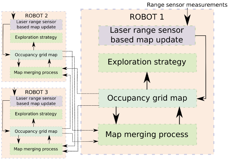
Fig. 1: A diagram of our mapping strategy. The arrows indicate information flow among components in our strategy.

In this paper, we present a distributed approach to the mapping problem that is scalable with the number of robots, relies only on local inter-robot communication, and does not require robots to have sophisticated sensing and computation capabilities. Figure 1 gives a schematic diagram of our mapping strategy. In our approach, robots explore an unknown environment while simultaneously building an occupancy grid map online from their own distance measurements and from maps communicated by other robots that they encounter. As in most occupancy grid mapping strategies, we assume that each robot is either capable of accurately estimating its pose or is equipped with a localization device. We present a distributed algorithm for sharing and fusing occupancy grid maps among robots in such a way that each robot’s map eventually converges to the same global map of the entire environment, which we prove using results on achieving consensus on time-varying graphs [14]. Our analysis of the distributed mapping algorithm is similar, in spirit, to the ones present in [15]. The robots do not need to have unique identities that are recognized by other robots in order to implement this map-sharing algorithm. Since all robots ultimately arrive at a consensus on the map, this map can be retrieved from a single arbitrary robot in the swarm, making the strategy robust to robot failures. We also introduce an exploration strategy that combines concepts from information theory [16] with Lévy walks, a type of random walk with step lengths distributed according to a power law that has been used as a model for efficient search strategies by both animals and robots [17]. We empirically show that this new exploration strategy, which we refer to as an information correlated Lévy walk (ICLW), enables a swarm of robots to explore a domain faster than if they use standard Lévy walks, thereby enabling them to map the domain more quickly. Finally, we illustrate that a technique based on topological data analysis, used for generating topological maps in our previous work [18], can also be used for adaptive thresholding of occupancy grid maps with a slight modification. The threshold distinguishes occupied grid cells from unoccupied cells in the map by applying tools from algebraic topology [19]. A significant difference between our earlier topological approach and the one presented in this paper is our use here of cubical complexes [20], a natural choice for grid maps, instead of simplicial complexes [21] We validate our mapping approach in 2D simulations of various environments with different sizes and layouts, using the mobile robot simulator Stage [22]. We also experimentally validate our approach with the commercially available TurtleBot 3 Burger robots.

In contrast to many multi-robot strategies for exploration and mapping, our approach is an identity-free strategy in that the robots are indistinguishable from one another; i.e., robots are agnostic to the individual identities of other robots with which they interact. This property is useful for mapping approaches using robotic swarms, since it facilitates the scalability of the approach with the number of robots and is robust to robot failures during task execution. In addition, unlike many multi-robot mapping strategies, our approach is suitable for robotic platforms with limited computational capabilities, which is a typical constraint on robots that are intended to be deployed in swarms since each robot should be relatively inexpensive. Notably, although the robots identify other robots within their sensing range as obstacles, our approach filters out these “false obstacles” when generating the map of the environment from the robots’ data. Also, our map merging approach guarantees that the map of each robot will eventually converge to the actual map of the domain, as long as the robots’ exploration strategy facilitates sufficient communication among the robots and coverage of the domain.

In our previous work, we developed different techniques for addressing swarm robotic mapping problems. In [23], we present a method for mapping GPS-denied environments using a swarm of robots with stochastic behaviors. Unlike this paper, the approach in [23] employs optimal control of partial differential equation models of the swarm population dynamics to estimate the map of the environment. Although the method in [23] only requires robot data on encounter times with features of interest, it is limited in application to domains with a few sparsely distributed features. The methodologies discussed in our previous works [24] and [18] estimate the number of obstacles in the domain and extract a topological map of the domain, respectively. Except for the procedure for adaptive thresholding of occupancy grid maps that is delineated in Section V, the work presented in this paper is novel and does not directly follow any of our previous works. Also, unlike our previous works, this mapping strategy computes the map online rather than offline.

In summary, the contributions of this paper are as follows:

• We present a new exploration strategy for robotic swarms that consists of Lévy walks influenced by information-theoretic metrics.

• We develop a completely decentralized strategy by which a swarm of robots without unique identities can generate an occupancy grid map of an unknown environment.

• We prove that each robot’s occupancy grid map asymptotically converges to a common map at an exponential rate.

• We extend our topological data analysis-based technique for adaptive thresholding of occupancy grid maps [24, 18, 25] to domains represented as cubical complexes, instead of simplicial complexes as in our prior work.

The remainder of the paper is organized as follows. Section II formally states the problem that we address and the associated assumptions. We describe our swarm exploration strategy in Section III and our occupancy grid mapping strategy and its analysis in Section IV. Section V outlines our TDA-based method for adaptive thresholding of occupancy grid maps and basic concepts from algebraic topology that are required to understand the technique. Section VI and Section VII present and discuss the results from simulations and robot experiments, respectively. The paper concludes with Section VIII.

TABLE I: Notation

Symbol	Description
$N_{R}$	Number of robots
$R^{i}$	Label of robot $i\in\{1,...,N_{R}\}$
$x^{i}$	$x$-coordinate of $R^{i}$ w.r.t to global frame
$y^{i}$	$y$-coordinate of $R^{i}$ w.r.t to global frame
$\theta^{i}$	Orientation of $R^{i}$ w.r.t to global frame
$z^{i,a}_{\tau}$	Measurement from $a^{th}$ laser range sensor of $R^{i}$ at time $\tau$
$\mathbf{x}^{i}_{\tau}$	Pose $[x^{i}~{}y^{i}~{}\theta^{i}]^{T}$ of $R^{i}$ at time $\tau$
$\mathbf{v}^{i}_{\tau}$	Linear velocity vector of $R^{i}$ at time instant $\tau$
$\mathbf{z}^{i}_{\tau}$	Vector of laser range sensor measurements of $R^{i}$ at time $\tau$
$M^{i}$	Occupancy grid map stored in $R^{i}$
$m^{i}_{j}$	$j^{th}$ grid cell of occupancy map $M^{i}$
$\mathbb{P}_{m^{i}_{j}}$	Probability that cell $m^{i}_{j}$ is occupied (occupancy probability)
$\mathbb{P}_{M^{i}}$	Probability that occupancy map $M^{i}$ is completely occupied
$\mathbf{\bar{P}}_{M^{i}}$	Set of occupancy probabilities $\left\{\mathbb{P}_{m^{i}_{j}}\right\}_{j=1}^{|M^{i}|}$
$s^{i}$	Constant speed of $R^{i}$
$\Delta t$	Time interval $[\tau~{}~{}\tau+T]$
$\mathbf{X}^{i}_{\Delta t}$	Pose sequence $[\mathbf{x}^{i}_{\tau}~{}\cdots~{}\mathbf{x}^{i}_{\tau^{\prime}}~{}\cdots~{}\mathbf{x}^{i}_{\tau+T}]$
$\mathbf{Z}^{i}_{\Delta t}$	Measurement sequence $[\mathbf{z}^{i}_{\tau},\cdots,\mathbf{z}^{i}_{\tau^{\prime}},\cdots,\mathbf{z}^{i}_{\tau+T}]$
$\mathbf{I}[\mathbf{A};\mathbf{B}|\mathbf{C}]$	Mutual information between random var.’s $\mathbf{A}$, $\mathbf{B}$ given $\mathbf{C}$
$<\mathbf{a}>$	Arithmetic mean of the elements in vector $\mathbf{a}$
$<\mathbf{a}>_{gm}$	Geometric mean of the elements in vector $\mathbf{a}$
$u(m_{j}^{i},\mathbf{x}^{i}_{k},\mathbf{z}^{i}_{k})$	Update rule that $R^{i}$ uses to assign $\mathbb{P}_{m^{i}_{j}}$
$\mathbb{G}(k)$	Undirected robot communication graph at time step $k$
$\mathbb{V}$	Vertex set of $\mathbb{G}(k)$, $\{1,...,N_{R}\}$ (robot indices)
$\mathbb{E}(k)$	Edge set of $\mathbb{G}(k)$ (pairs of robots that can communicate)
$\mathbb{A}(k)$	Adjacency matrix associated with $\mathbb{G}(k)$
$\mathbb{N}_{k}^{i}$	Neighbors of $R^{i}$ (can communicate with $R^{i}$) at time step $k$

II Problem Statement

We address the problem of estimating the map of an unknown domain $D\subset\mathbb{R}^{d}$ using distance measurements acquired by a swarm of $N_{R}$ robots while exploring the domain. We consider bounded, closed, path-connected domains that contain static obstacles. Although in this paper we only address the case $d=2$, it is straightforward to extend our procedure to the case $d=3$. Table I lists the definitions of variables that we use throughout the paper for ease of reference.

II-A Robot capabilities

We assume that the robots have the following capabilities. Each robot acquires noisy distance measurements using a laser range sensor such as a SICK LMS200 laser rangefinder [26]. Using this data, a robot can detect its distance to obstacles and other robots within its local sensing radius and perform collision avoidance maneuvers if needed. Each robot broadcasts its stored map information, and other robots that are within a distance $b_{r}$ of the robot can use this information to update their own maps. We assume that each robot can estimate its own pose with no uncertainty. It is important to note that the robots are not equipped with any sensors that can distinguish between obstacles and other robots. The robots also do not have unique identifiers.

II-B Representation of the domain as an occupancy grid map

Every robot models the unknown environment as an occupancy grid map, which does not require any a priori information about the size of the domain and can be expanded as the robot acquires new distance measurements [1]. Each grid cell of an occupancy grid map is associated with a value that encodes the probability of the cell being occupied by an obstacle. Let $M^{i}_{t}$ denote the occupancy grid map stored by robot $R^{i}$ at time $t$, where $i\in\{1,...,N_{R}\}$. We specify that each robot discretizes the domain with the same resolution. At this resolution, a map of the entire domain $D\subset\mathbb{R}^{2}$ is discretized uniformly into $|D|$ grid cells, labeled $m^{i}_{1},...,m^{i}_{|D|}$. During the mapping procedure, each robot augments its map based on its own distance measurements and map information from nearby robots, effectively adding grid cells to its current map. The occupancy grid map of robot $i$ at time $t$ is represented by the grid cells $m^{i}_{1},...,m^{i}_{|M^{i}_{t}|}$, where $|M^{i}_{t}|$ denotes the number of grid cells in the robot’s map at time $t$. Henceforth, we will usually drop the subscript $t$ from $M_{t}^{i}$ to simplify the notation, with the understanding that the map $M^{i}$ depends on time.

Let $\mathbf{m}^{i}_{j}$, $j\in\{1,...,|M^{i}|\}$, be a Bernoulli random variable that takes the value 1 if the region enclosed by grid cell $m^{i}_{j}$ is occupied by an obstacle, and 0 if it is not. Thus, $\mathbb{P}(\mathbf{m}^{i}_{j}=1)$ is the probability that grid cell $m^{i}_{j}$ is occupied, called its occupancy probability. A standard assumption for occupancy grid maps is the independence of the random variables $\mathbf{m}^{i}_{j}$. As a result, the probability that map $M^{i}$ belongs to a domain which is completely occupied is given by $\mathbb{P}(M^{i})=\prod_{j=1}^{|M^{i}|}\mathbb{P}(\mathbf{m}^{i}_{j}=1)$. For the sake of brevity, we will use the notation $\mathbb{P}_{m^{i}_{j}}\equiv\mathbb{P}(\mathbf{m}^{i}_{j}=1)$ and $\mathbb{P}_{M^{i}}\equiv\mathbb{P}(M^{i})$ throughout the paper. We also define the set $\mathbf{\bar{P}}_{M^{i}}=\left\{\mathbb{P}_{m^{i}_{j}}\right\}_{j=1}^{|M^{i}|}$, which is the collection of the occupancy probabilities of all grid cells in map $M^{i}$. Finally, the entropy $H(M^{i})$ of the map $M^{i}$, which quantifies the uncertainty in the map, is defined as [1]:

$$H(M^{i})=\sum_{j=1}^{|M^{i}|}\sum_{k=\left\{0,1\right\}}\mathbb{P}(\mathbf{m}^{i}_{j}=k)\log_{2}\left(\mathbb{P}(\mathbf{m}^{i}_{j}=k)\right)$$ (1)

II-C Mapping approach and evaluation

Our mapping approach consists of the following steps. All robots explore the domain simultaneously using the random walk strategy that is defined in Section III. While exploring, each robot updates its occupancy grid map with its own distance measurements, broadcasts this map to neighboring robots, and then modifies its map with the maps transmitted by these neighboring robots using a predefined discrete-time, consensus-based protocol, which is discussed in Section IV. We prove that the proposed protocol guarantees that every robot’s map will eventually converge to a common map. A technique for post-processing the occupancy grid map based on topological data analysis (TDA) is presented in Section V. We evaluate the performance of our mapping approach according to two metrics: (1) the percentage of the entire domain that is mapped after a specified amount of time, and (2) the entropy of the final occupancy grid map, as defined in Equation 1.

III Exploration Based On Information Correlated Lévy Walks

In this section, we describe the motion strategy used by robots to explore the unknown domain. Exploration strategies for robotic swarms generally use random, guided, or information-based approaches [27, 1, 9, 28]. Random exploration approaches are often based on Brownian motion (e.g., [29, 30, 31]) or Lévy walks (e.g., [32, 33, 17, 34, 35]), which facilitate uniform dispersion of the swarm throughout a domain from any initial distribution. Moreover, these approaches do not rely on centralized motion planning or extensive inter-robot communication, which can scale poorly with the number of robots in the swarm. Information-based approaches, such as [36, 37], guide robots in the direction of maximum information gain based on a specified metric, which can increase the efficiency of exploration compared to random approaches. Mutual information (or information gain), a measure of the amount of information that one random variable contains about another [16], is a common metric used to assess the information gain that results from a particular action by a robot. This metric can be used to predict the increase in certainty about a state of the robot’s environment that is associated with a new sensor measurement by the robot.

We specify that each robot in the swarm performs a combination of random and information-based exploration approaches, in order to benefit from the advantages of both types of strategies. We describe the implementation of ICLW in this section. Our exploration strategy does not require the robots to identify or use any information from their neighboring robots while covering the domain; therefore, it is an identity-free strategy.

To execute a Lévy walk, a robot repeatedly chooses a new heading and moves at a constant speed [38] in that direction over a random distance that is drawn from a heavy-tailed probability distribution function $p(l)$, of the form

$$p(l)\propto l^{-\alpha},$$ (2)

where $\alpha$ is the Lévy exponent. The case $1<\alpha<3$ signifies a scale-free superdiffusive regime, in which the expected displacement of a robot performing the Lévy walk over a given time is much larger than that predicted by random walk models of uniform diffusion. This superdiffusive property disperses the robots quickly toward unexplored regions.

In contrast to standard Lévy walks (SLW), in which the agent’s heading is uniformly random, we define the heading chosen by the robot before each step in the Lévy walk as the direction that maximizes the robot’s information gain about the environment. This is computed as the direction that maximizes the mutual information between the robot’s current occupancy grid map and the distance measurements that it is likely to obtain when it moves in that direction, based on the forward measurement model of a laser range sensor [1] over a finite time horizon. These measurements are expected to decrease the entropy of the robot’s occupancy grid map, defined in Equation 1. Therefore, the computed robot heading is more likely to direct the robot to unexplored regions than a uniformly random heading. The calculation of this heading is described in the following subsections.

III-A Laser range sensor forward measurement model

We assume that the laser range sensor of each robot $R^{i}$ has $N_{l}$ laser beams that all lie in a plane parallel to the base of the robot. The distance measurement obtained by the $a^{th}$ laser beam of robot $R^{i}$ at time $\tau$ is a random variable that will be denoted by $z^{i,a}_{\tau}$. The random vector of all distance measurements obtained by robot $R^{i}$ at time $\tau$ is represented as $\mathbf{z}^{i}_{\tau}=[z^{i,1}_{\tau}~{}\cdots~{}z^{i,a}_{\tau}~{}\cdots~{}z^{i,N_{l}}_{\tau}]^{T}$.

Define $s_{min}$ and $s_{max}$ as the minimum and maximum possible distances, respectively, that can be measured by the laser range sensor. In addition, let $\delta$ denote the actual distance of an obstacle that is intersected by the $a^{th}$ laser beam of robot $R^{i}$. The Gaussian distribution function with mean $\mu$ and variance $\sigma^{2}$ will be written as $\mathcal{N}(\mu,\sigma^{2})$. We define the probability density function of the distance measurement $z^{i,a}_{\tau}$, given the actual distance $\delta$, as the forward measurement model presented in [36],

$$\mathbb{P}(z^{i,a}_{\tau}~{}|~{}\delta)=\begin{cases}\mathcal{N}(0,\sigma^{2}),&\ \delta\leq s_{min}\\ \mathcal{N}(s_{max},\sigma^{2}),&\ \delta\geq s_{max}\\ \mathcal{N}(\delta,\sigma^{2}),&\text{otherwise,}\end{cases}$$ (3)

where $\sigma^{2}$ is the variance of the range sensor noise in the radial direction of the laser beam. Although this model does not incorporate range sensor noise in the direction perpendicular to the laser beam, the experimental results in [36] and our results in Section VII demonstrate that the model captures sufficient noise characteristics for generating accurate maps from the sensor data.

III-B Robot headings based on mutual information

The mutual information between two random variables $\mathbf{A}$ and $\mathbf{B}$ is defined as the Kullback-Leibler distance [16] between their joint probability distribution, $\mathbb{P}(\mathbf{A},\mathbf{B})$, and the product of their marginal probability distributions, $\mathbb{P}(\mathbf{A})\mathbb{P}(\mathbf{B})$:

$$\mathbf{I}[\mathbf{A};\mathbf{B}]=\mathbb{K}\mathbb{L}\mathbb{D}\left(\mathbb{P}(\mathbf{A},\mathbf{B})||\mathbb{P}(\mathbf{A})\mathbb{P}(\mathbf{B})\right)$$ (4)

This quantity measures how far $\mathbf{A}$ and $\mathbf{B}$ are from being independent. In other words, $\mathbf{I}[\mathbf{A};\mathbf{B}]$ quantifies the amount of information that $\mathbf{B}$ contains about $\mathbf{A}$, and vice versa. For example, if $\mathbf{A}$ and $\mathbf{B}$ are independent random variables, then no information about $\mathbf{A}$ can be extracted from the outcomes of $\mathbf{B}$, and consequently, $\mathbf{I}[\mathbf{A};\mathbf{B}]=0$. On the other hand, if $\mathbf{A}$ is a deterministic function of $\mathbf{B}$, then the entropies of both random variables are equal to the expected value of $-\log_{2}(\mathbb{P}(\mathbf{A}))$, and $\mathbf{I}[\mathbf{A};\mathbf{B}]$ is equal to this quantity, which is its maximum value.

During each step in its random walk, every robot performs the following computations and movements. A new step may be initiated either when the robot completes its previous step, or when the robot encounters an obstacle (or other robot) during its current step. Suppose that the next step by robot $R^{i}$ starts at time $\tau$. At this time, the robot computes the duration $T$ of the step by generating a random distance based on the Lévy distribution (Equation 2) and dividing this distance by its speed $s^{i}$, which is constant. Also at time $\tau$, the robot computes the velocity $\mathbf{v}^{i}_{\Delta t}$ that it will follow during the time interval $\Delta t\ \coloneqq\ [\tau~{}~{}\tau+T]$. This computation involves several variables, which we introduce here. The pose of robot $R^{i}$ at time $\tau$ is denoted by $\mathbf{x}^{i}_{\tau}$ (see Table I). We define a sequence of this robot’s poses during the time interval $\Delta t$ as $\mathbf{X}^{i}_{\Delta t}\ \coloneqq\ [\mathbf{x}^{i}_{\tau}~{}\cdots~{}\mathbf{x}^{i}_{\tau^{\prime}}~{}\cdots~{}\mathbf{x}^{i}_{\tau+T}]$, where $\tau^{\prime}\in\Delta t$. We also define $\mathbf{Z}^{i}_{\Delta t}\ \coloneqq\ [\mathbf{z}^{i}_{\tau},\cdots,\mathbf{z}^{i}_{\tau^{\prime}},\cdots,\mathbf{z}^{i}_{\tau+T}]$ as a set of random vectors modeling laser range sensor measurements that the robot is expected to receive as it moves during this time interval. At time $\tau$, robot $R^{i}$ calculates its velocity $\mathbf{v}^{i}_{\Delta t}$ as the solution ${}^{*}\mathbf{v}^{i}_{\Delta t}$ to the following optimization problem, with the objective function defined as in [36, 39] :

$$^{*}\mathbf{v}^{i}_{\Delta t}=\underset{\left\|\mathbf{v}^{i}_{\Delta t}\right\|=s^{i},~{}\angle\mathbf{v}^{i}_{\Delta t}\in[-\pi,\pi]}{\mbox{arg max}}\frac{\mathbf{I}[{M^{i}};~{}\mathbf{Z}^{i}_{\Delta t}\ |\ \mathbf{X}^{i}_{\Delta t}]}{C(\mathbf{v}^{i}_{\Delta t})},$$ (5)

where $\mathbf{I}[{M^{i}};~{}\mathbf{Z}^{i}_{\Delta t}\ |\ \mathbf{X}^{i}_{\Delta t}]$ represents the mutual information between the robot’s occupancy grid map and its distance measurements given a sequence of the robot’s poses. The term $C(\mathbf{v}^{i}_{\Delta t})$ in Equation 5 penalizes the robot for large deviations from its current heading when multiple velocities generate different paths with the same mutual information. We define $C(\mathbf{v}^{i}_{\Delta t})=\|\mathbf{v}^{i}_{\Delta t}-\mathbf{v}^{i}_{\tau}\|/s^{i}+\varphi$, where $\varphi$ is a small positive constant which ensures that $C(\mathbf{v}^{i}_{\Delta t})$ is strictly positive. For the computations in the paper, we chose $\varphi=\pi/72$ rad, or 2.5^∘. Based on the current occupancy grid map $M^{i}$ of robot $R^{i}$ and its set of expected poses $\mathbf{X}^{i}_{\Delta t}$ under its velocity command $\mathbf{v}^{i}_{\Delta t}$, $R^{i}$ can compute the probability distribution of its laser range sensor measurements using the forward measurement model Equation 3.

Before we elaborate on the details of solving the optimization problem described in Equation 5, we present the intuition behind our argument that maximizing the objective function in Equation 4 tends to direct a robot to unexplored regions according to its current map. By the definition of mutual information (see Equation 7), $\mathbf{I}[{M^{i}};~{}\mathbf{Z}^{i}_{\Delta t}\ |\ \mathbf{X}^{i}_{\Delta t}]$ quantifies the expected reduction in the uncertainty of a robot’s map due to the sensor measurements received by the robot during its motion. In essence, $\mathbf{I}[{M^{i}};~{}\mathbf{Z}^{i}_{\Delta t}\ |\ \mathbf{X}^{i}_{\Delta t}]$ captures the expected amount of entropy reduced in the robot’s map $M^{i}$ based on the likely measurements ($\mathbf{Z}^{i}_{\Delta t}$) that the robot would obtain if it followed a trajectory $\mathbf{X}^{i}_{\Delta t}$. Therefore, maximizing $\mathbf{I}[{M^{i}};~{}\mathbf{Z}^{i}_{\Delta t}\ |\ \mathbf{X}^{i}_{\Delta t}]$ for different trajectories ($\mathbf{X}^{i}_{\Delta t}$) yields the trajectory that decreases the uncertainty in the robot’s map by the largest amount. There is an equal chance for a grid cell in an unexplored region to be free or occupied by an obstacle. Since the entropy of a Bernoulli random variable is highest when its probability of occurrence is $0.5$, the occupancy probabilities of the grid cells in the unexplored region have the highest entropy (uncertainty). Thus, maximizing $\mathbf{I}[{M^{i}};~{}\mathbf{Z}^{i}_{\Delta t}\ |\ \mathbf{X}^{i}_{\Delta t}]$ will generate trajectories that direct the robot toward unexplored regions based on the information contained in its map.

III-C Computing mutual information

In this section, we describe the computation of the objective function in Equation 5 and discuss techniques for solving the associated optimization problem. We first focus on computing $\mathbf{I}[M^{i};z^{i,a}_{\tau}]$, the mutual information between the measurement $z^{i,a}_{\tau}$ obtained by the $a^{th}$ laser beam of robot $R^{i}$ at time $\tau$ and the robot’s current occupancy grid map $M^{i}$. Grid cells in the map that do not intersect the beam do not to contribute to the mutual information. Hence, the task of computing $\mathbf{I}[M^{i};z^{i,a}_{\tau}]$ reduces to computing $\mathbf{I}[\mathbf{c}^{i,a}_{\tau};z^{i,a}_{\tau}]$, where $\mathbf{c}^{i,a}_{\tau}$ is the collection of Bernoulli random variables $\mathbf{m}_{j}^{i}$ modeling the occupancy of grid cells in the map of robot $R^{i}$ that are intersected by the $a^{th}$ beam at time $\tau$. This quantity is defined as [39]:

$$\mathbf{I}[\mathbf{c}^{i,a}_{\tau};z^{i,a}_{\tau}]=\int_{z\in z^{i,a}_{\tau}}\sum_{c\in\mathbf{c}^{i,a}_{\tau}}\mathbb{P}(c,z)\log_{2}\left(\frac{\mathbb{P}(c,z)}{\mathbb{P}(c)\mathbb{P}(z)}\right)dz,$$ (6)

where $\mathbb{P}(c,z)$ is the joint probability distribution of $c$ and $z$, and $\mathbb{P}(c)$ and $\mathbb{P}(z)$ are the probability distributions of the occupancy probabilities of the intersected grid cells and the range sensor distance measurements, respectively. We show in Appendix A that $\mathbf{I}[\mathbf{c}^{i,a}_{\tau};z^{i,a}_{\tau}]$ can be expressed as:

$$\mathbf{I}[\mathbf{c}^{i,a}_{\tau};z^{i,a}_{\tau}]=-\int_{z^{i,a}_{\tau}}\mathbb{P}(z)\log_{2}(\mathbb{P}(z))dz+K,$$ (7)

where $K=-\log(\sqrt{2\pi}\sigma)-0.5$. Since $K$ is not a function of the map or the distance measurements, it does not affect the solution to the optimization problem in Equation 5 and therefore does not need to be included in this problem.

The effect of $\mathbf{c}^{i,a}_{\tau}$ on $\mathbf{I}[\mathbf{c}^{i,a}_{\tau};z^{i,a}_{\tau}]$ is through the probability distribution $\mathbb{P}(z)$ in Equation 7. We now compute this distribution. From the forward measurement model Equation 3, $\mathbb{P}(z)$ is completely determined by the distance $\delta$ from the laser range sensor to the closest occupied cell in $\mathbf{c}^{i,a}_{\tau}$. Let $e_{p}$ denote a binary sequence of length $|\mathbf{c}^{i,a}_{\tau}|$ in which each of the first $p-1$ elements is 0 and the $p^{th}$ element is 1. The remainder of the elements in the sequence can be either 0 or 1. This sequence is a possible realization of $\mathbf{c}^{i,a}_{\tau}$, in which the first $p-1$ intersected grid cells are unoccupied, the $p^{th}$ cell is occupied, and the remaining cells may or may not be occupied. For compactness of notation, we define $e_{0}$ as the sequence in which all elements are 0; that is, no intersected grid cells are occupied. Then, we have that

$$\mathbb{P}(z)=\sum_{p=0}^{|\mathbf{c}^{i,a}_{\tau}|}\mathbb{P}(z~{}|~{}\mathbf{c}^{i,a}_{\tau}=e_{p})\mathbb{P}(\mathbf{c}^{i,a}_{\tau}=e_{p})$$ (8)

We direct the reader to [36, 37] for a detailed description of such sensor models.

We can now extend our computation of the mutual information for a single distance measurement at a given time to $\mathbf{I}[M^{i};\mathbf{Z}^{i}_{\Delta t}\ |\ \mathbf{X}^{i}_{\Delta t}]$, the mutual information for all distance measurements taken by robot $R^{i}$ over a sequence of times. Since the exact computation of this quantity is intractable, we adopt a common technique used in the robotics literature: we select several laser beams on the robot and assume that the measurements from these beams are independent of one another [40, 37]. We define $\mathcal{Z}^{i}_{\Delta t}$ as the set of distance measurements obtained at times $\tau^{\prime}\in\Delta t$ from the selected laser beams on robot $R^{i}$, indexed by $a^{\prime}\in\{1,...,N_{l}\}$. Then, we can approximate $\mathbf{I}[M^{i};\mathbf{Z}^{i}_{\Delta t}\ |\ \mathbf{X}^{i}_{\Delta t}]$ as the following sum over $\mathcal{Z}^{i}_{\Delta t}$:

$$\mathbf{I}[M^{i};\mathbf{Z}^{i}_{\Delta t}\ |\ \mathbf{X}^{i}_{\Delta t}]~{}\approx\sum_{z^{i,a^{\prime}}_{\tau^{\prime}}\in\mathcal{Z}^{i}_{\Delta t}}\mathbf{I}[M^{i};z^{i,a^{\prime}}_{\tau^{\prime}}]$$ (9)

In general, finding $\mathcal{Z}^{i}_{\Delta t}\subseteq\mathbf{Z}^{i}_{\Delta t}$ that best approximates the formula in Equation 9 is an NP-hard problem [36]. Therefore, no approximation algorithm can be designed to find this $\mathcal{Z}^{i}_{\Delta t}$ in polynomial time. However, generating $\mathcal{Z}^{i}_{\Delta t}$ using greedy algorithms has shown promising results [40, 37, 36].

Here, we specify the following procedure for a robot to solve the optimization problem in Equation 5 in order to compute the heading that maximizes its information gain. The robot implements the greedy algorithm in [40], which selects the laser beams having an information gain above a predefined threshold, to find $\mathcal{Z}^{i}_{\Delta t}$ in Equation 9. The expression in Equation 9 is used to approximate $\mathbf{I}[M^{i};\mathbf{Z}^{i}_{\Delta t}\ |\ \mathbf{X}^{i}_{\Delta t}]$, where each term $\mathbf{I}[M^{i};z^{i,a^{\prime}}_{\tau^{\prime}}]$ is equal to $\mathbf{I}[\mathbf{c}^{i,a^{\prime}}_{\tau^{\prime}};z^{i,a^{\prime}}_{\tau^{\prime}}]$, defined in Equation 7. The expression for $\mathbb{P}(z)$ in Equation 7 is computed from Equation 8, and Equation 7 is numerically integrated. The robot employs a greedy algorithm to find a suboptimal solution to the optimization problem in Equation 5. Specifically, the value of the objective function in Equation 5 is computed along different headings, and the robot selects the heading corresponding to the maximum value. It is straightforward to show that the computational cost for evaluating the objective function along a heading has an upper bound $\mathcal{O}(|M^{i}|\cdot|\mathcal{Z}^{i}_{\Delta t}|)$, where $|\mathcal{Z}^{i}_{\Delta t}|$ is the cardinality of $\mathcal{Z}^{i}_{\Delta t}$. For the simulations and experiments in this paper, the objective function was computed along eight different headings, which enabled the robots to accurately map the domain without requiring an excessive computational load on each robot.

An alternate approach to solving the optimization problem in Equation 5 is to compute the gradient of the objective function and define the robot’s heading as the direction of gradient ascent. However, since the computations are performed on a discrete occupancy grid map, it is not clear that the objective function has a well-defined gradient. Although prior attempts have been made to compute the gradients of information-based objective functions under particular assumptions [39, 41], the gradient computation relies on numerical techniques such as finite difference methods.

IV Occupancy grid map updates by each robot

While exploring the environment, each robot updates its occupancy grid map based on its laser range sensor measurements and the occupancy grid map information broadcast by robots that are within a distance $b_{r}$. In this section, we describe how robot $R^{i}$ updates $\mathbf{\bar{P}}_{M^{i}}$, the collection of occupancy probabilities of all cells in its map, using both its distance measurements and the sets $\mathbf{\bar{P}}_{M^{\hat{n}}},\hat{n}\in\mathbb{N}_{\tau}^{i}$, where $\mathbb{N}_{\tau}^{i}$ denotes the set of robots that are within distance $b_{r}$ of robot $R^{i}$ at time $\tau$. We present a discrete-time, consensus-based protocol for modifying the occupancy map of each robot and prove that this protocol guarantees that all robots eventually arrive at a consensus on the map of the environment. As explained in Section IV-B, our method for updating the occupancy map is resilient to false positives, meaning that even if a robot incorrectly assigns a high occupancy probability $\mathbb{P}_{m^{i}_{j}}$ to a free grid cell $j$ due to noise in its distance measurement, the impact of this noisy measurement on $\mathbb{P}_{m^{i}_{j}}$ is eventually mitigated due to the averaging effect of our map modification protocol. Since occupancy grid mapping algorithms require the robots’ pose information, we assume that each robot can estimate its own pose using an accurate localization technique.

IV-A Occupancy map updates based on distance measurements

The forward sensor measurement model Equation 3 represents the probability that a robot obtains a particular distance measurement given the robot’s map of the environment and the robot’s pose. The parameter $\delta$ in the model can be computed from the robot’s map and pose. Commonly used occupancy grid mapping algorithms [1, 3] use an inverse sensor measurement model to update the occupancy probabilities of the grid cells. This type of model gives the probability that a grid cell is occupied, given the laser range sensor measurements and the pose of the robot. Although forward sensor measurement models can be easily derived for any type of range sensor, inverse sensor measurement models are more useful for occupancy grid algorithms [1]. Methods such as supervised learning algorithms and neural networks have been used to derive inverse sensor models based on a range sensor’s forward model [42]. Pathak et al. [43] describe a rigorous approach to deriving an analytical inverse sensor model for a given forward sensor model. Although inverse sensor models derived from forward sensor models can be used to efficiently estimate an occupancy grid map, it is difficult to develop a distributed version of such models, since either their computation is performed offline [42] or the mapping between the forward and inverse sensor models is nonlinear [43]. These difficulties preclude us from exploiting these techniques in our mapping approach.

Instead, we propose a heuristic inverse range sensor model for which a distributed version can be easily derived. We specify that each robot estimates its pose and obtains distance measurements at discrete time steps, to reflect the fact that sensor measurements are recorded at finite sampling rates. Let $\mathbf{x}^{i}_{k}$ denote the pose of robot $R^{i}$ at time step $k$, and let $\mathbf{z}^{i}_{k}$ be the vector of its distance measurements at this time step. Our inverse sensor model, which we refer as an update rule, is a function $u:(m^{i}_{j},\mathbf{x}^{i}_{k},\mathbf{z}^{i}_{k})\rightarrow[0,1]$. This function assigns an occupancy probability to grid cell $m_{j}^{i}$ based on the robot’s pose and all of its distance measurements at time step $k$. Robot $R^{i}$ uses this function to modify $\mathbf{\bar{P}}_{M^{i}}$ based on its distance measurements. We define the update rule in terms of a function $l:(m^{i}_{j},\mathbf{x}^{i}_{k},z^{i,a}_{k})\rightarrow[0,1]$, which assigns an occupancy probability to grid cell $m^{i}_{j}$ based on the robot’s pose and its $a^{th}$ laser beam’s distance measurement at time step $k$. The function can be applied only to those grid cells $m^{i}_{j}$ that are intersected by the $a^{th}$ beam at time step $k$.

We define $l$ as one of two functions, $l_{r}$ and $l_{u}$, depending on whether the robot estimates that its $a^{th}$ laser beam is reflected ($l_{r}$) or not reflected ($l_{u}$). These functions depend on $s^{a}_{m^{i}_{j}}$, the distance from the center of cell $m^{i}_{j}$ to the $a^{th}$ laser range sensor of robot $R^{i}$, and constants $p_{a}$, $p_{f}$, and $p_{hit}$. The functions $l$, $l_{r}$, and $l_{u}$ are defined as follows:

$$l(m^{i}_{j},\mathbf{x}^{i}_{k},z^{i,a}_{k})=\begin{cases}l_{r}(s^{a}_{m^{i}_{j}},z^{i,a}_{k})&\ z^{i,a}_{k}\leq s_{max}-\sigma\\ l_{u}(s^{a}_{m^{i}_{j}})&\ z^{i,a}_{k}>s_{max}-\sigma\\ \end{cases}$$ (10)

$$l_{r}(s^{a}_{m^{i}_{j}},z^{i,a}_{k})=\begin{cases}\frac{p_{a}-p_{f}}{s_{max}}s^{a}_{m^{i}_{j}}+p_{f}&s^{a}_{m^{i}_{j}}<z^{i,a}_{k}-\sigma\\ p_{hit}&z^{i,a}_{k}-\sigma\leq s^{a}_{m^{i}_{j}}\leq z^{i,a}_{k}+\sigma\end{cases}$$ (11)

$$l_{u}(s^{a}_{m^{i}_{j}})=\begin{cases}\frac{p_{a}-p_{f}}{s_{max}}s^{a}_{m^{i}_{j}}+p_{f}&s^{a}_{m^{i}_{j}}<s_{max}-\sigma\\ p_{a}&s_{max}-\sigma\leq s^{a}_{m^{i}_{j}}\leq s_{max}+\sigma\\ \end{cases}$$ (12)

Figure 2 illustrates the functions $l_{r}$ and $l_{u}$ that are defined in Equation 11 and Equation 12, respectively.

Our heuristic inverse sensor model can model laser range sensors for which the noise in the range measurements is predominantly in the radial direction of the laser beams. We defined our inverse sensor model based on the physically realistic assumption that given a range measurement, the grid cells closer to the robot have a lower occupancy probability than the grid cells farther away. In our model, if a laser range measurement $z^{i,a}_{k}$ is obtained, then the occupancy probability of each grid cell along the radial direction of the laser beam increases with its distance from the sensor, until this distance is within $\sigma$ units of the measurement $z^{i,a}_{k}$. The model assumes that a grid cell whose distance from the sensor is in the interval $[z^{i,a}_{k}-\sigma,z^{i,a}_{k}+\sigma]$ belongs to an obstacle. On the contrary, if no laser range measurement is obtained, then the model assumes that a grid cell at a distance less than $s_{max}-\sigma$ from the sensor is likely to be unoccupied by an obstacle. We selected parameter values for the model for which the robots generated reasonably accurate maps in our simulations and experiments. Alternatively, one could estimate the parameter values by fitting the model to real measurements from laser range sensors.

Given the function $l$ in Equation 10, we now specify the update rule function $u$ according to the following procedure. We define $\zeta$ as the set of distance measurements $z_{k}^{i,a}$ at time step $k$ that are recorded by laser beams that either intersect grid cell $m^{i}_{j}$ or are reflected by an obstacle that covers $m^{i}_{j}$. If $\zeta=\emptyset$, meaning that none of the measurements in $\mathbf{z}^{i}_{k}$ provide any information about $m^{i}_{j}$, then we set $u(m^{i}_{j},\mathbf{x}^{i}_{k},\mathbf{z}^{i}_{k})=1$ to make the update rule well-defined for such grid cells. Otherwise, we set $u(m^{i}_{j},\mathbf{x}^{i}_{k},\mathbf{z}^{i}_{k})$ to the maximum value of $l(m^{i}_{j},\mathbf{x}^{i}_{k},z)$ over all measurements $z\in\zeta$.

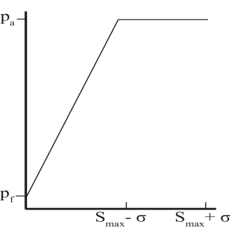
(a) unreflected model

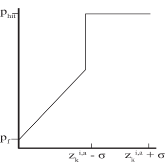
(b) reflected model

Fig. 2: Illustrative plots of the functions (a) $l_{u}$ and (b) $l_{r}$. The $x$-axis in both plots measures $s^{a}_{m^{i}_{j}}$, the distance between the $a^{th}$ laser range sensor of robot $R^{i}$ and any grid cell $m^{i}_{j}$ that intersects the beam from this laser, which yields the distance measurement $z^{i,a}_{k}$ at time step $k$.

IV-B Consensus-based occupancy grid map sharing

In this section, we describe a discrete-time, consensus-based protocol by which each robot modifies its occupancy map using the maps that are broadcast by neighboring robots. We prove that each robot’s map asymptotically converges to the occupancy grid map that best represents the domain by using analysis techniques for linear consensus protocols over time-varying graphs, which have been well-studied in the literature [44, 45, 46, 14]. The main results of these works assume the existence of a time interval over which the union of the graphs contains a spanning tree, which is required in order to reach consensus. In particular, we apply results from [14] on average consensus over time-varying graph topologies in a discrete-time setting.

We begin with an overview of average consensus over time-varying graphs, using graph-theoretic notation from [47]. We define $\mathbb{G}(k)\ =\ \left(\mathbb{V},\mathbb{E}(k)\right)$ as an undirected time-varying graph with $n$ vertices, $\mathbb{V}=\{1,...,n\}$, and a set of undirected edges $\mathbb{E}(k)$ at time step $k$. In our scenario, $\mathbb{G}(k)$ defines the communication network of the robots at time step $k$, in which the vertices represent the robots, $\mathbb{V}=\{1,...,N_{R}\}$, and each edge $(i,\hat{n})\in\mathbb{E}(k)$ indicates that robots $R^{i}$ and $R^{\hat{n}}$ are within broadcast range of each other at time step $k$ and can therefore exchange information.

Let $\mathbb{A}(k)=[a_{ij}(k)]\in\mathbb{R}^{n\times n}$ be the adjacency matrix associated with graph $\mathbb{G}(k)$ at time step $k$, where $a_{ij}(k)$ denotes the element in the $i^{th}$ row and $j^{th}$ column of $\mathbb{A}(k)$. In this matrix, $a_{ij}(k)\neq 0$ if and only if an edge exists between vertices $i$ and $j$ at time step $k$, and $a_{ij}(k)=0$ otherwise. The set of neighbors of vertex $i$ at time step $k$, defined as $\mathbb{N}_{k}^{i}=\left\{\hat{n}~{}|~{}(i,\hat{n})\in\mathbb{E}(k),~{}i\neq\hat{n}\right\}$, contains the vertices $j$ for which $a_{ij}(k)\neq 0$. Suppose that at time step $k$, each vertex $i$ is associated with a real scalar variable $x_{i}(k)$. At every time step, the vertex updates its value of $x_{i}(k)$ to a weighted linear combination of its neighbors’ values and $x_{i}(k)$, where the weights are the corresponding values of $a_{ij}(k)$. Then the vector $\mathbf{x}(k)=[x_{1}(k)~{}...~{}x_{n}(k)]^{T}$ evolves according to the discrete-time dynamics $\mathbf{x}(k+1)=\mathbb{A}(k)\mathbf{x}(k)$. If $\lim_{k\rightarrow\infty}x_{j}(k)=\frac{1}{n}\sum_{i=1}^{n}x_{i}(0)$ for all $j\in\mathbb{V}$, then the vertices are said to have achieved average consensus. It is proved in [14, Theorem 1] that the dynamics of $\mathbf{x}(k)$ converge asymptotically to average consensus if $\mathbb{A}(k)$ is a doubly stochastic matrix, meaning that each of its rows and columns sums to 1, and if there exists a time interval for which the union of graphs over this interval is connected. We will use these results to prove an important result on our protocol for occupancy map sharing.

We now define the protocol by which robot $R^{i}$ updates $\mathbf{\bar{P}}_{M^{i}}$, the occupancy probabilities of all grid cells in its map $M^{i}$, based on its neighbors’ occupancy maps, its current occupancy map, and its distance measurements. It is important to note that the maps do not contain any information about the robots that broadcasted them. We specify that the occupancy probability $\mathbb{P}_{m^{i}_{j}}(k)$ of every grid cell $m_{j}^{i}$ in the map $M^{i}$ at time step $k$ is updated at the next time step as follows:

$$\mathbb{P}_{m^{i}_{j}}(k+1)=u(m^{i}_{j},\mathbf{x}^{i}_{k},\mathbf{z}^{i}_{k})~{}\cdot\prod_{\hat{n}\in\mathbb{N}^{i}_{k}\cup i}\left(\mathbb{P}_{m^{\hat{n}}_{j}}(k)\right)^{a_{i\hat{n}}(k)}.$$ (13)

We introduce the vector $\mathbf{u}_{j}[k]=[u(m^{1}_{j},\mathbf{x}^{1}_{k},\mathbf{z}^{1}_{k})~{}\cdots~{}u(m^{N_{R}}_{j},\mathbf{x}^{N_{R}}_{k},\mathbf{z}^{N_{R}}_{k})]^{T}$; that is, each entry of $\mathbf{u}_{j}[k]$ is the value of the function $u$ that a robot uses to compute the occupancy probability of the $j^{th}$ cell in its map at time step $k$. We use the notation $\mathbf{u}_{j}[k]\neq\mathbf{1}$ to indicate that at least one element of $\mathbf{u}_{j}[k]$ is not 1; i.e., at least one robot obtains distance measurements at time step $k$ that yield information about the $j^{th}$ cell. We also define the set $\mathbf{d}$ as the sequence of time steps $d\in\{0,1,...,\infty\}$ for which $\mathbf{u}_{j}[d]\neq\mathbf{1}$.

We make the following assumptions about the robots’ communication network, map updates, and distance measurements. These assumptions are required to prove the main theoretical result of this paper, Theorem 1.

Assumption 1.

There exists a time interval over which the union of robot communication graphs $\mathbb{G}(k)$ is connected.

In reality, it is difficult to prove that this assumption holds true for robots that explore arbitrary domains. However, it is reasonable to suppose that the assumption is satisfied for scenarios where a relatively high density of robots results in frequent robot interactions, or where the robots’ communication range is large with respect to the domain area.

Assumption 2.

Suppose that at time step $k$, robot $R^{i}$ has a nonempty set of neighbors $\mathbb{N}^{i}_{k}$, indexed by $r=\{1,...,|\mathbb{N}^{i}_{k}|\}$. Then robot $R^{i}$ modifies its occupancy map according to Equation 13 using the map from its $r^{th}$ neighbor $R^{\hat{n}}$ at each time step $k+r$, and setting the nonzero $a_{ij}$ values at time steps $k^{\prime}=k+r-1$ to $a_{ii}(k^{\prime})=0.5$, $a_{i\hat{n}}(k^{\prime})=0.5$. If robot $R^{i}$ has no neighbors at time step $k$, i.e., $\mathbb{N}^{i}_{k}=\emptyset$, then it sets $a_{ii}(k)=1$ in Equation 13.

To illustrate, if robot $R^{i}$ has three neighbors $\mathbb{N}_{k}^{i}=\{R^{p},R^{q},R^{r}\}$ at time step $k$ that all communicate their maps $M^{p},M^{q},M^{r}$ to $R^{i}$, then $R^{i}$ can use Equation 13 to update its map $M^{i}$ with map $M^{p}$ at time step $k+1$, map $M^{q}$ at time step $k+2$, and map $M^{r}$ at time step $k+3$. If a fourth robot $R^{s}$ enters the neighborhood of $R^{i}$ between time steps $k$ and $k+3$, $R^{i}$ updates its map with map $M^{s}$ at time step $k+4$. The choice of $a_{ij}(k)$ values ensures that the adjacency matrix $\mathbb{A}(k)$ is doubly stochastic at each time step $k$.

Assumption 3.

The set $\mathbf{d}$ is finite.

This assumption is made to enable the proof of Theorem 1, rather than to describe an inherent property of the mapping strategy. In practice, the assumption can be realized by programming the robots to ignore their laser range sensor measurements after receiving a predefined number of them, although we did not need to enforce this assumption explicitly in our simulations and experiments.

To facilitate our analysis, we include an additional assumption on the robots’ distance measurements. We define the accessible grid cells for robot ${R}^{i}$ as the set of grid cells in ${M}^{i}$ whose occupancy probabilities can be inferred by $R^{i}$ from its laser range sensor measurements. This set includes all unoccupied grid cells and the grid cells along the periphery of obstacles. The $a^{th}$ cell in this set is denoted by $m^{i}_{a}$. The set of inaccessible grid cells contains all other cells in $M^{i}$, and the $\bar{a}^{th}$ cell in this set is denoted by $m^{i}_{\bar{a}}$.

Assumption 3A. In the limiting case where the robots explore the environment for an infinite amount of time, each robot $R^{i}$ uses the value of the function $u(m^{i}_{a},\mathbf{x}^{i}_{k},\mathbf{z}^{i}_{k})$ at exactly one time step $k$ per accessible grid cell $m^{i}_{a}$ to infer the occupancy probability of that cell. We define $\bar{u}^{i}_{a}=u(m^{i}_{a},\mathbf{x}^{i}_{k},\mathbf{z}^{i}_{k})$ for this $k$, which may be chosen as any time step at which $u(m^{i}_{a},\mathbf{x}^{i}_{k},\mathbf{z}^{i}_{k})\neq 1$. We assume that there always exists such a time step $k$; i.e., that each robot obtains distance measurements that provide information about every accessible grid cell.

We can now state the main result of this paper, which uses the following definitions. The vector of all robots’ occupancy probabilities for the $j^{th}$ cell at time step $k$ is written as $\mathbb{P}_{m_{j}}[k]=[\mathbb{P}_{m^{1}_{j}}(k)~{}...~{}\mathbb{P}_{m^{N_{R}}_{j}}(k)]^{T}$. In addition, $<\cdot>_{gm}$ denotes the geometric mean operator, defined as $<\mathbf{q}>_{gm}=\sqrt[n]{q_{1}\cdot q_{2}\cdot...\cdot q_{n}}$ for a vector $\mathbf{q}=[q_{1}~{}q_{2}~{}...~{}q_{n}]^{T}$.

Theorem 1.

If each robot $R^{i}$ updates its occupancy grid map according to Equation 13, then under Assumption 1-Assumption 3 (excluding Assumption 3A), we have that

$$\lim_{k\rightarrow\infty}\mathbb{P}_{m^{i}_{j}}(k)~{}=~{}<\mathbb{P}_{m_{j}}[0]>_{gm}\hskip 2.84526pt\cdot\hskip 2.84526pt\prod_{d\in\mathbf{d}}<\mathbf{u}_{j}[d]>_{gm}.$$ (14)

For an inaccessible grid cell $m^{i}_{\bar{a}}$, Equation 14 reduces to

$$\lim_{k\rightarrow\infty}\mathbb{P}_{m^{i}_{\bar{a}}}(k)~{}=~{}<\mathbb{P}_{m_{\bar{a}}}[0]>_{gm}.$$ (15)

In addition, under Assumption 3A, the asymptotic value of $\mathbb{P}_{m^{i}_{a}}$ for an accessible grid cell $m^{i}_{a}$ can be derived from Equation 14 as

$$\lim_{k\rightarrow\infty}\mathbb{P}_{m^{i}_{a}}(k)~{}=~{}<\mathbb{P}_{m_{a}}[0]>_{gm}\cdot<[\bar{u}^{1}_{a}~{}\cdots~{}\bar{u}^{N_{R}}_{a}]^{T}>_{gm},$$ (16)

Furthermore, Equation 14, Equation 15, and Equation 16 converge exponentially to their respective limits.

Proof.

See Appendix B. ∎

Theorem 1 states that under the map modification protocol Equation 13, the occupancy probability $\mathbb{P}_{m^{i}_{j}}$ of every grid cell $m^{i}_{j}$ in the map of each robot $R^{i}$ will converge exponentially to a value that is proportional to $\prod_{d\in\mathbf{d}}<\mathbf{u}_{j}[d]>_{gm}$. For each inaccessible grid cell, Equation 15 dictates that the occupancy probability converges to the constant $<\mathbb{P}_{m_{\bar{a}}}[0]>_{gm}$, If we set $\mathbb{P}_{m^{i}_{j}}(0)=1$ for each robot $R^{i}$, then this constant equals one, which is an accurate occupancy probability since the cell is occupied. By Equation 16, the occupancy probability of each accessible grid cell $m^{i}_{a}$ will asymptotically tend to the geometric mean of $[\bar{u}^{1}_{a}~{}\cdots~{}\bar{u}^{N_{R}}_{a}]^{T}$ if the proportionality constant $<\mathbb{P}_{m_{a}}[0]>_{gm}$ is 1, which also occurs if we initialize $\mathbb{P}_{m^{i}_{j}}(0)=1$ for each robot $R^{i}$. Since the occupancy probability $\mathbb{P}_{m^{i}_{j}}$ of each grid cell $m^{i}_{j}$ ultimately converges to the geometric mean of occupancy probabilities computed by every robot, and the effect of outliers in the data is greatly dampened in the geometric mean [48], the resulting $\mathbb{P}_{m^{i}_{j}}$ reasonably represents the true occupancy of the grid cell, even if a few robots record highly noisy or inaccurate measurements.

We note that although our analysis specifically guarantees asymptotic convergence of the robots’ maps to the actual map, our simulation and experimental results in Section VI and Section VII show that the maps indeed converge in finite time within reasonable accuracy.

V Post-Processing of Occupancy Grid Maps

Since all robots’ occupancy grid maps eventually converge to a common occupancy map, in theory only a single robot needs to be retrieved to obtain this map. In this section, we propose a technique for post-processing the grid cell occupancy probabilities from the retrieved robot(s) to infer the most likely occupancy grid map of the environment. We note that this technique can be applied to occupancy grid maps that are generated through any mapping procedure. A common approach to this inference problem is the Maximum A Posterior (MAP) mapping procedure [1], which computes the occupancy grid map with the maximum probability of occurrence based on the occupancy probability of each grid cell in the map. In general, the MAP procedure is posed as an optimization problem, and the solution is computed using gradient-based hill climbing methods. This approach is computationally expensive, since gradient ascent must be performed from different initial conditions to escape local maxima and the search space is exponential in the number of grid cells (for a given set of $n$ grid cells, there are $2^{n}$ possible occupancy grid maps [1]).

Here, we present an alternative approach that is based on techniques from topological data analysis (TDA) [49], which uses the mathematical framework of algebraic topology [19]. In practice, the time complexity of our procedure is linear in the number of grid cells $(\mathcal{O}(|M^{i}|))$ [18]. In Section V-A, we present an overview of relevant concepts from TDA and algebraic topology. An in-depth treatment of these subjects can be found in [49, 19, 20, 50]. We then describe our TDA-based occupancy grid mapping procedure in Section V-B.

V-A Algebraic topology and Topological Data Analysis (TDA)

In recent years, considerable progress has been made in using tools from algebraic topology to estimate the underlying structure and shape of data [51], which aids in efficient analysis of the data using statistical techniques such as regression [21]. Topological data analysis (TDA) is a collection of algorithms for performing coordinate-free topological and geometric analysis of noisy data. In most applications, the data consists of noisy samples of an intensity map that is supported on a Euclidean domain. The set of these data is referred as a point cloud. The dominant topological features of the Euclidean domain associated with the point cloud can be computed using persistent homology [21], a key concept in TDA. A compact graphical representation of this information can be presented using barcode diagrams [50] and persistence diagrams [21].

A topological space $\mathbf{T}$ can be associated with an infinite sequence of vector spaces called homology groups, denoted by $H_{t}(\mathbf{T})$, $t=0,1,2,\dots$. Each of these vector spaces encodes information about a particular topological feature of $\mathbf{T}$. The dimension of $H_{t}(\mathbf{T})$, defined as the Betti number $\beta_{t}$ [50], is a topological invariant that represents the number of independent topological features encoded by $H_{t}(\mathbf{T})$. Additionally, $\beta_{t}$ gives the number of independent $t$-dimensional cycles in $\mathbf{T}$. For example, if $\mathbf{T}$ is embedded in $\mathbb{R}^{2}$, denoted by $\mathbf{T}\hookrightarrow\mathbb{R}^{2}$, then $\beta_{0}$ and $\beta_{1}$ are the number of connected components in $\mathbf{T}$ and number of holes in $\mathbf{T}$, respectively.

In contrast to our previous works [24, 18], here we consider topological spaces that admit a cubical decomposition rather than a simplicial decomposition and use cubical homology rather than simplicial homology. The fundamental unit of a cubical complex is an elementary interval [20], a closed interval $\mathtt{I}\subset\mathbb{R}$ of the form $\mathtt{I}=[l,~{}l+1]$ (a nondegenerate interval) or $\mathtt{I}=[l,~{}l]$ (a degenerate interval) for some $l\in\mathbb{Z}$. A cube or elementary cube $\mathbb{Q}\subset\mathbb{R}^{d}$ is constructed from a finite product of elementary intervals $\mathtt{I}_{t}$, $\mathbb{Q}=\prod_{t=1}^{d}\mathtt{I}_{t}$ [20]. If $\mathbb{Q}$ and $\mathbb{O}$ are elementary cubes and $\mathbb{Q}\subset\mathbb{O}$, then $\mathbb{Q}$ is a face of $\mathbb{O}$. For a topological space $\mathbf{T}$, let a $t$-cube $\square_{t}$ be a continuous map $\square_{t}:[0,1]^{t}\rightarrow\mathbf{T}$ [52]. A $t$-cube has $2t$ faces, each of which is a ($t-1$)-dimensional cube. A cubical complex $\mathbb{K}$ is a union of $t$-cubes for which the faces of each cube are all in $\mathbb{K}$ and the intersection of any two cubes $\square_{t}$ and $\square^{\prime}_{t}$ is either the empty set or a common face of both $\square_{t}$ and $\square^{\prime}_{t}$.

Suppose that $\iota,\eta\in\mathbb{K}$. We use the notation $\eta\leq\iota$ to indicate that $\eta$ is a face of $\iota$. Let $f:\mathbb{K}\to\mathbb{R}$ be a function for which $\eta\leq\iota$ implies that $f(\eta)\leq f(\iota)$. Then $f^{-1}((-\infty,\varpi])$ is a cubical complex denoted by $\mathbb{K}_{\varpi}$, and $\varpi_{1}\leq\varpi_{2}$ implies that $\mathbb{K}_{\varpi_{1}}\subseteq\mathbb{K}_{\varpi_{2}}$, yielding a filtration [20] of cubical complexes with $\varpi$ as its filtration parameter. The persistent homology can be generated by varying the value of $\varpi$ and computing the basis of the homology group vector spaces (the homology generators) for each cubical complex corresponding to the value of $\varpi$. A barcode diagram represents $H_{t}(\mathbf{T})$ in terms of its homology generators and can be used to determine persistent topological features of the topological space $\mathbf{T}$. Figure 3 gives an example of a barcode diagram for a cubical complex. The diagram plots a set of horizontal line segments whose $x$-axis spans a range of filtration parameter values and whose $y$-axis shows the homology generators in an arbitrary ordering. The number of arrows in the diagram indicates the count of persistent topological features of $\mathbf{T}$. Specifically, the number of arrows in each homology group corresponds to the number of topological features that are encoded by that group.

Fig. 3: An example barcode diagram of a filtration constructed from a cubical complex. The shaded regions contain the two-dimensional elementary cubes (squares). The arrows in $H_{0}$ and $H_{1}$ indicate the persistent topological features over a range of values of the filtration parameter. The arrows show that the cubical complex has one persistent topological feature corresponding to each homology group $H_{0}$ and $H_{1}$.

V-B Classifying occupied and unoccupied grid cells with adaptive thresholding

We now describe our technique for distinguishing occupied grid cells from unoccupied grid cells by applying the concept of persistent homology to automatically find a threshold based on the occupancy probabilities $\mathbb{P}_{m^{i}_{j}}$ in a map $M^{i}$. This TDA-based technique provides an adaptive method for thresholding an occupancy grid map of a domain that contains obstacles at various length scales. In this approach, we threshold $\mathbb{P}_{m^{i}_{j}}$ at various levels, compute the numbers of topological holes (obstacles) in the domain corresponding to each level of thresholding, and identify the threshold value above which topological features persist.

As described in Section V-A, a filtration of cubical complexes $\mathbb{K}_{\varpi}$ with filtration parameter $\varpi$ can be used to compute the persistent homology. In order to be consistent with the definition of a filtration, we set $\mathbb{P}_{m^{i}_{j}}=1$ for unexplored grid cells $m^{i}_{j}$. We define the filtration parameter $\varpi$ as a threshold for identifying unoccupied grid cells $m^{i}_{j}$ according to $\mathbb{P}_{m^{i}_{j}}<\varpi$. A filtration is constructed by creating cubical complexes $\mathbb{K}_{\varpi}$ for a sequence of increasing $\varpi$ values. Each complex $\mathbb{K}_{\varpi}$ is defined as the union of all $2$-cubes $\square_{2}$ whose vertices $\square_{0}$ are the centers of grid cells $m^{i}_{j}$ for which $\mathbb{P}_{m^{i}_{j}}<\varpi$.

Next, a barcode diagram is extracted from the filtration and used to identify the number of topological features in the domain, which is given by the number of arrows in each homology group. The threshold $\varpi_{cls}$ for classification of the grid cells as occupied or unoccupied is defined as the minimum value of $\varpi$ for which all the topological features are captured by the corresponding cubical complex $\mathbb{K}_{\varpi}$. In the barcode diagram, there exists no horizontal line segment other than the arrows in any of the homology groups for all $\varpi>\varpi_{cls}$. The value of $\varpi_{cls}$ can be computed as the maximum value of $\varpi$ that is spanned by the terminating barcode segments in all the homology groups.

The persistent homology computations were performed using the C++ program Perseus [53], and the barcode diagrams were generated using MATLAB. Since Perseus only accepts integers as filtration parameters, the $\mathbb{P}_{m^{i}_{j}}$ values of each map $M^{i}$ were scaled between 0 and 255 prior to being used as input to the computations. In our simulations and experiments, we restricted the persistent homology computations to dimensions zero and one since the domains being mapped were two-dimensional.

(a)

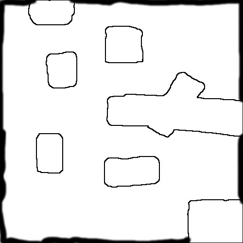
(b)

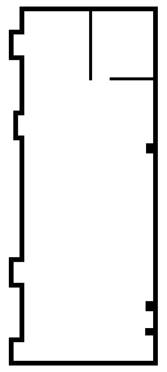
(c)

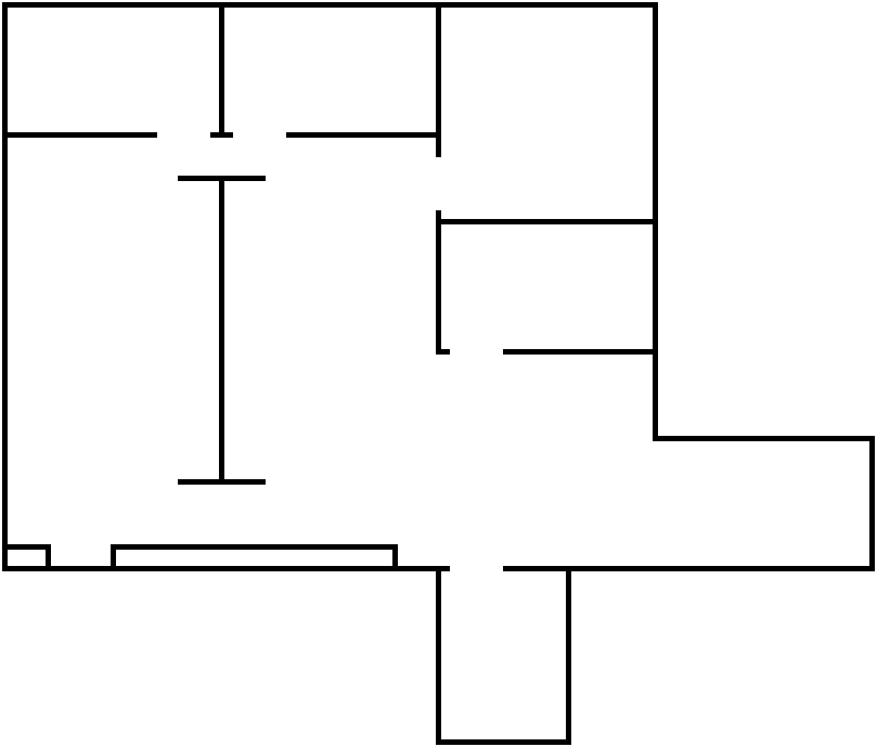
(d)

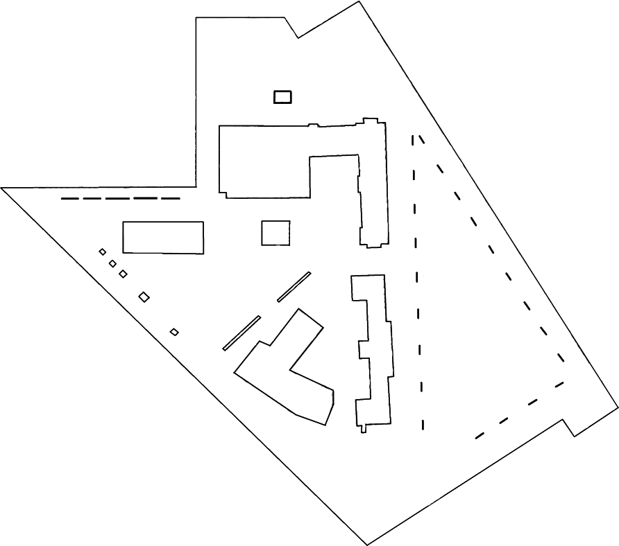
(e)

Fig. 4: Simulated environments, all obtained from [54]. The dimensions of the minimum bounding rectangle of each environment are given in parentheses. (a) An unobstructed environment (16 m $\times$ 16 m); (b) a cave environment (16 m $\times$ 16 m); (c) floor plan of a robotics laboratory at the University of Auckland (40 m $\times$ 20 m); (d) floor plan of an autonomy laboratory (40 m $\times$ 30 m); (e) University of Freiburg campus (90 m $\times$ 80 m).

(a)

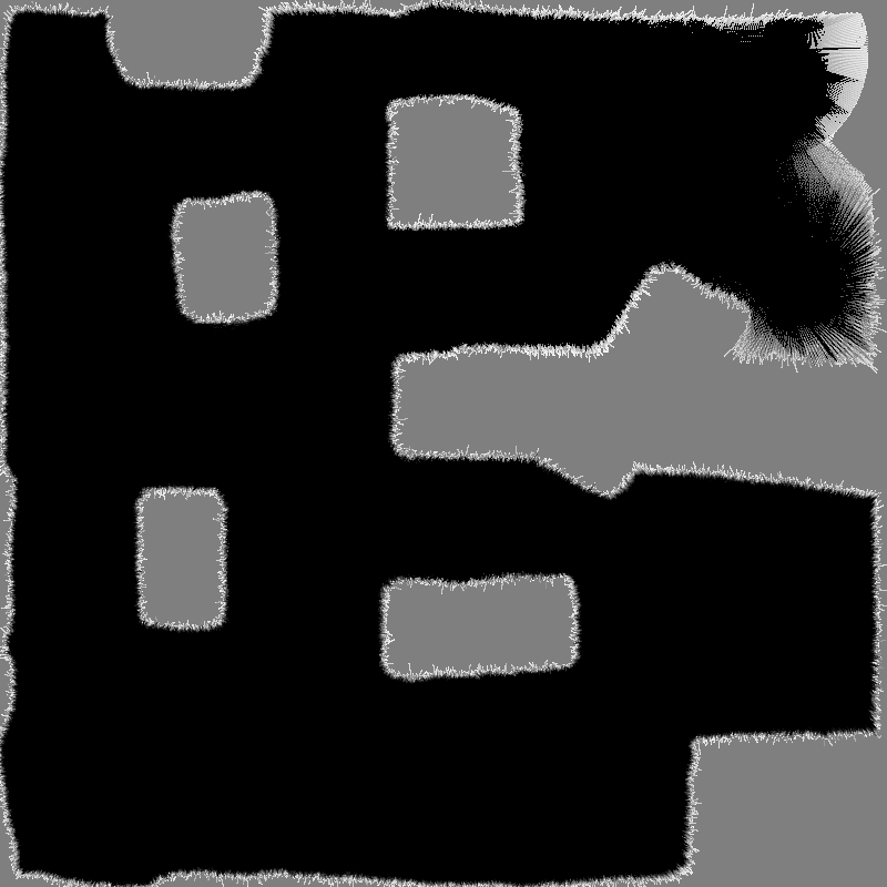
(b)

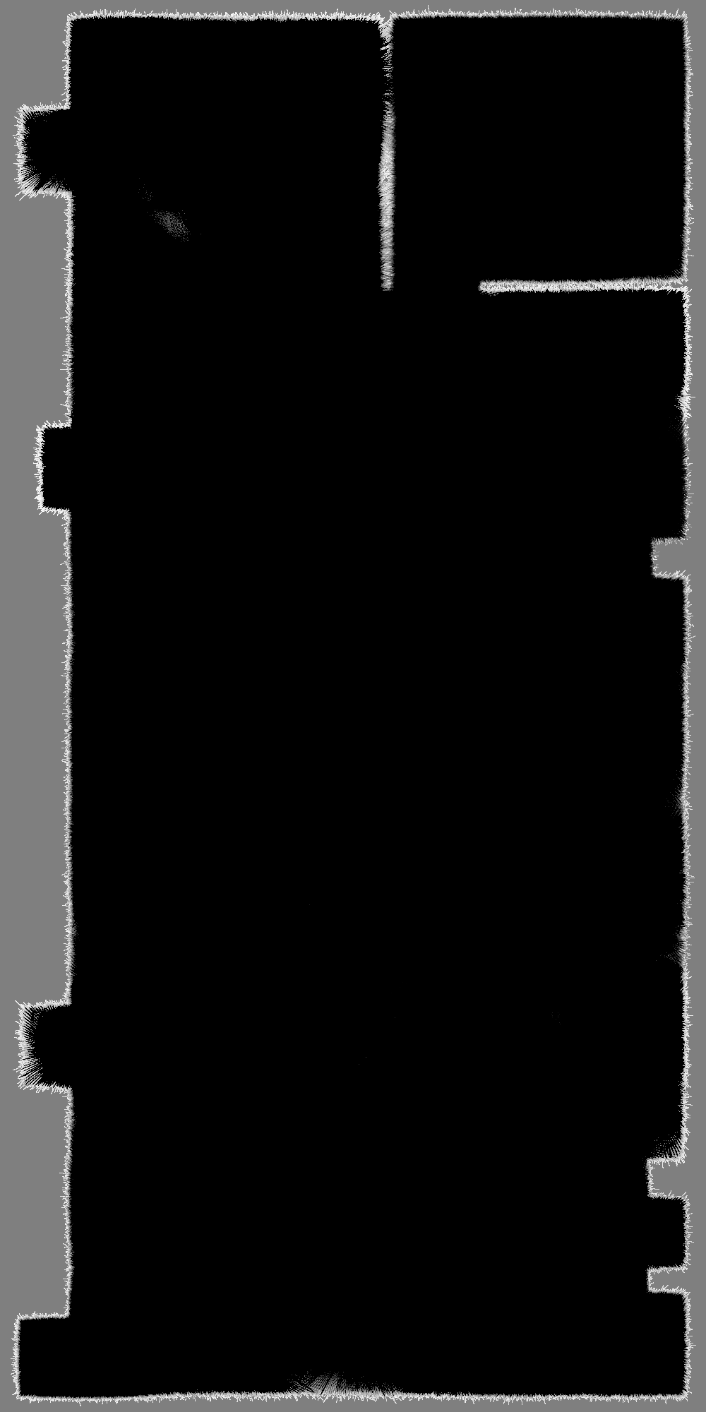
(c)

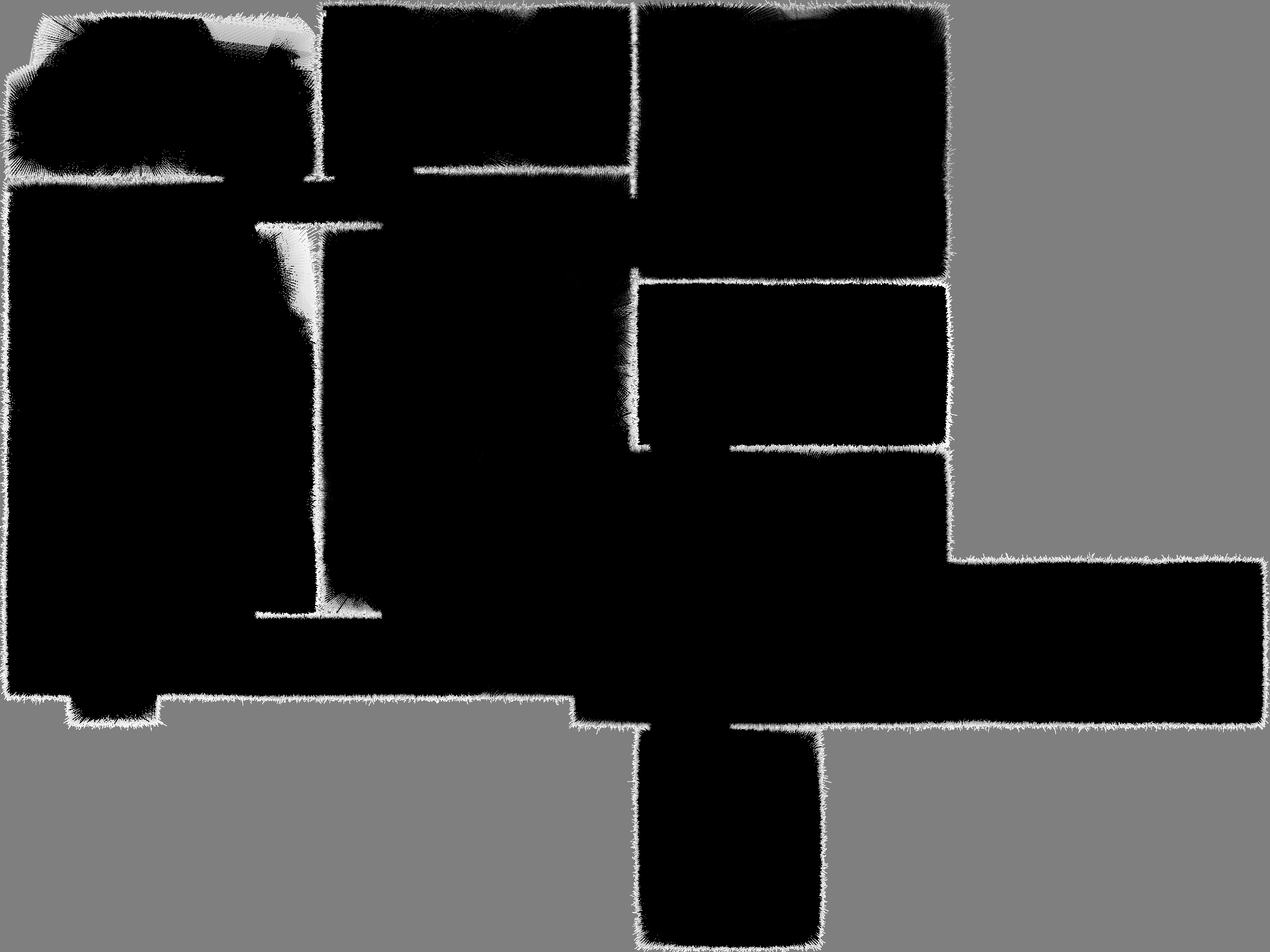
(d)

(e)

Fig. 5: Occupancy grid maps of the environments in (a) Figure 4(a), (b) Figure 4(b), (c) Figure 4(c), (d) Figure 4(d), and (e) Figure 4(e). Each map is generated by an arbitrary member of a swarm of $N_{R}$ robots that explore the environment for $t_{f}$ seconds: (a) $N_{R}=1$, $t_{f}=1800$ s; (b) $N_{R}=5$, $t_{f}=1200$ s; (c) $N_{R}=10$, $t_{f}=1500$ s; (d) $N_{R}=20$, $t_{f}=900$ s; and (e) $N_{R}=50$, $t_{f}=3600$ s. Gray regions that correspond to obstacles and the exterior of the domain are unexplored. Within the explored parts of the domain, dark regions contain grid cells with low occupancy probabilities ($\mathbb{P}_{m^{i}_{j}}\approx 0.1$ in black regions), and light regions have high occupancy probabilities ($\mathbb{P}_{m^{i}_{j}}\approx 0.9$ in white regions).

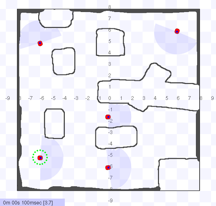
(a) $0$ s

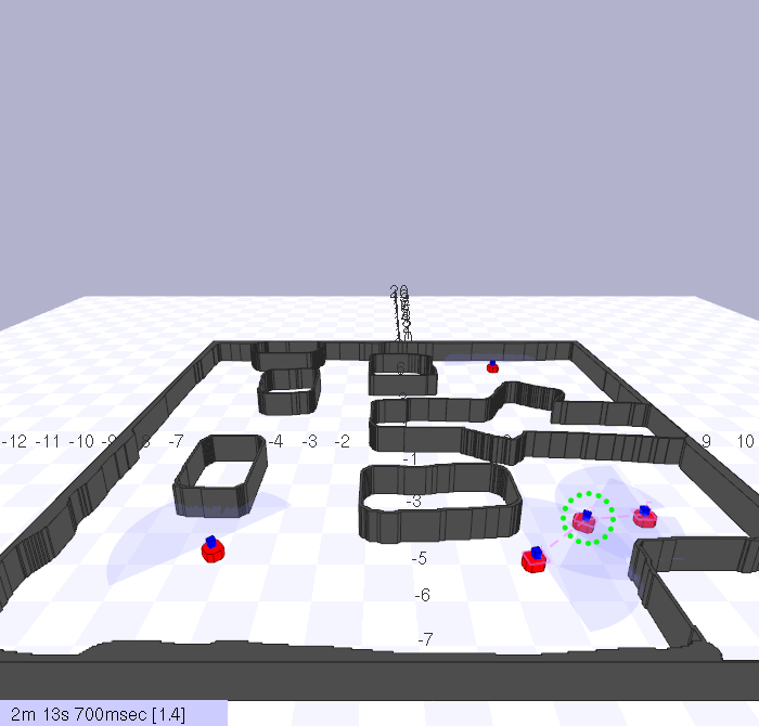
(b) $133$ s

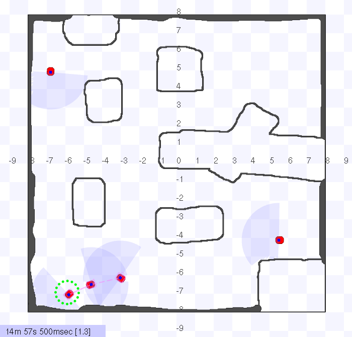
(c) $897$ s

Fig. 6: Snapshots of a simulation of five robots exploring the cave environment (Figure 4(b)) at the times given in the captions. Figure 6(a), and Figure 6(c) show overhead views of the environment, while Figure 6(b) shows perspective view. The blue shaded region emanating from each robot displays the range of its laser sensors. A red dotted line between two robots in Figure 6(b) indicates that the robots can communicate with each other.

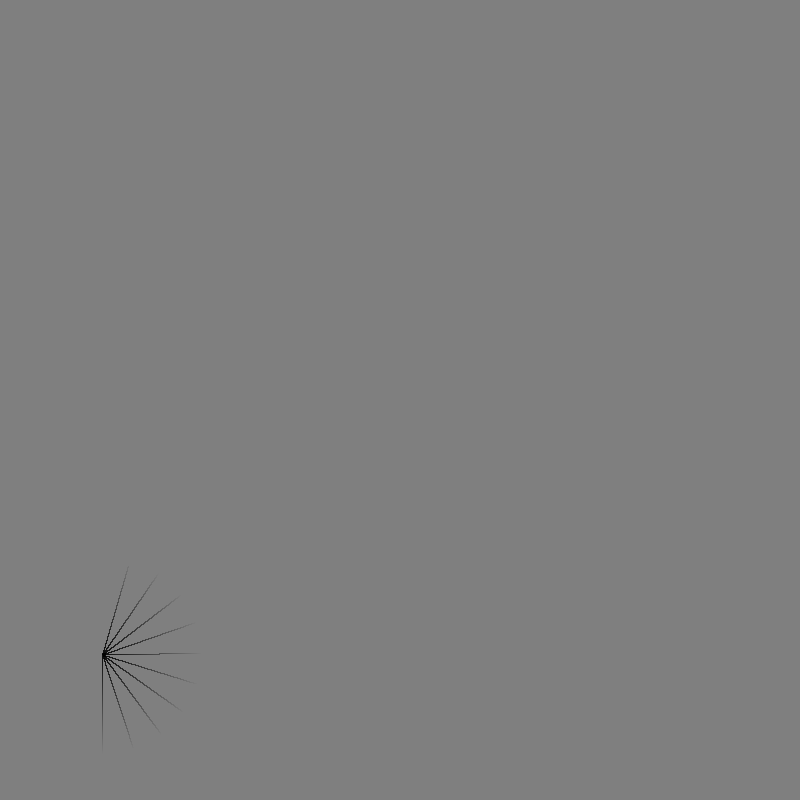
(a) $0$ s

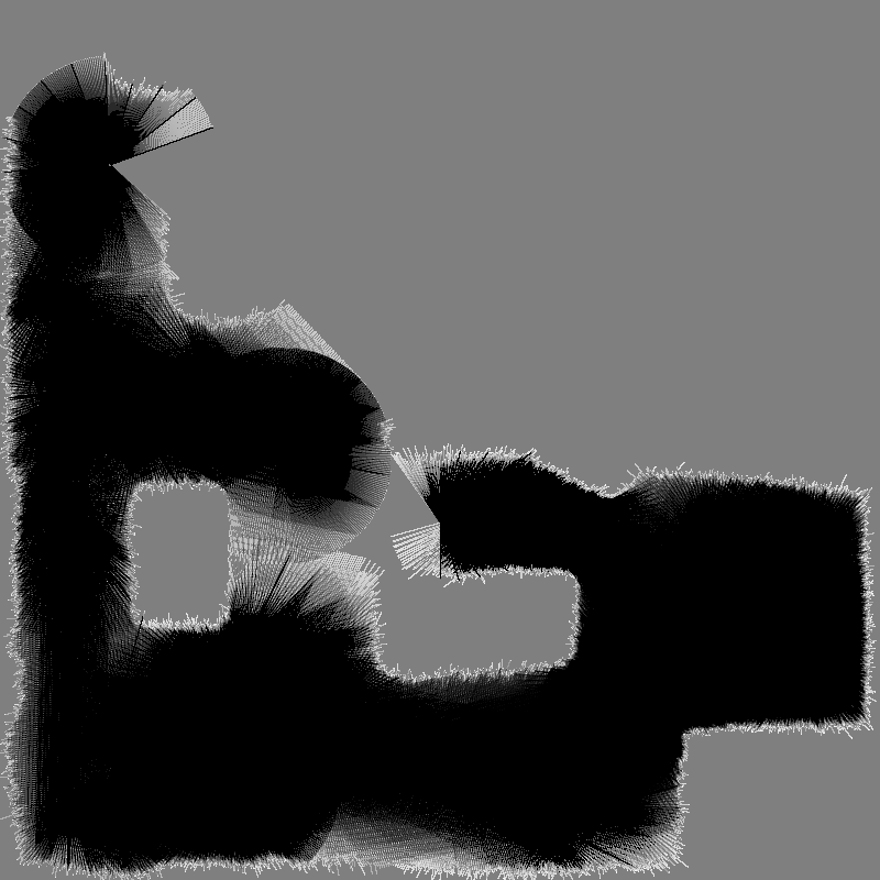
(b) $133$ s

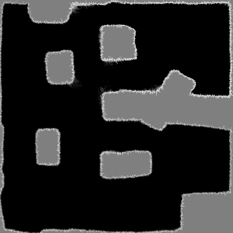
(c) $897$ s

Fig. 7: The occupancy grid map generated by the robot inside the green dotted circle in the snapshots in Figure 6 at the times of these snapshots.

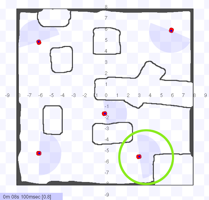
(a)

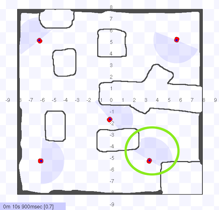
(b)

Fig. 8: The robot inside the green circle (a) detects an obstacle, then (b) follows a new heading computed from Eq. 5.

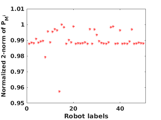
Fig. 9: Consensus over maps. The metric $\|\mathbf{P}_{M^{i}}\|_{2}/\max_{i}\|\mathbf{P}_{M^{i}}\|_{2}$, where $\mathbf{P}_{M^{i}}$ is the set $\mathbf{\bar{P}}_{M^{i}}$ in matrix form, for each robot $R^{i}$ in a swarm of 50 robots that explore the environment in Figure 4(e) for $t_{f}=3600$ s.

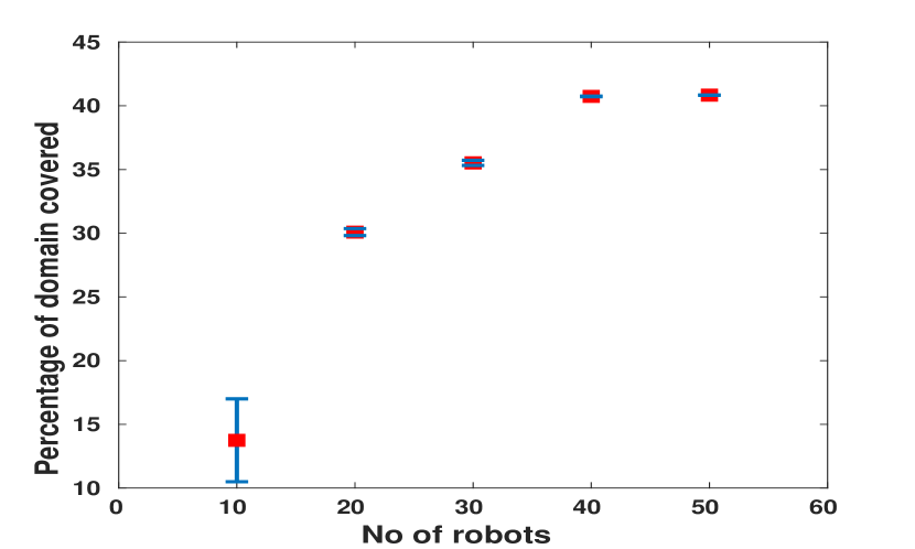
Fig. 10: Coverage vs. swarm size. Percentage of the environment in Figure 4(e) that is covered by swarms of different sizes after $t_{f}=3600$ s. Red dots indicate the median percentage over 10 simulations, and error bars show the $25^{th}$ and $75^{th}$ percentiles.

(a) Map from robot $R^{1}$

(b) Map from robot $R^{4}$

(c) Map from robot $R^{8}$

(d) Map from robot $R^{9}$

(e) Map from robot $R^{12}$

(f) Map from robot $R^{14}$

(g) Map from robot $R^{37}$

(h) Map from robot $R^{45}$

Fig. 11: Occupancy grid maps computed by 8 members of a swarm of $50$ robots after exploring the environment in Figure 4(e) for 3600 s.

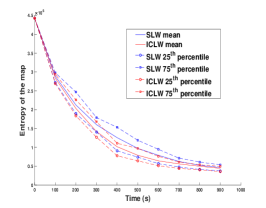
(a) Unobstructed environment

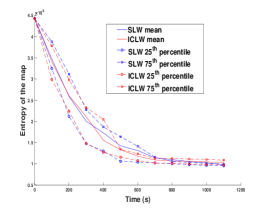
(b) Cave environment

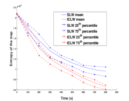
(c) Autonomy laboratory

Fig. 12: Time evolution of the entropy $H(M^{i})$, computed using Equation 1, of occupancy maps $M^{i}$, $i=1,...,N_{R}$, from simulations of: (a) $N_{R}=5$ robots mapping the unobstructed environment in Figure 4(a); (b) $N_{R}=5$ robots mapping the cave environment in Figure 4(b); and (c) $N_{R}=20$ robots mapping the autonomy laboratory in Figure 4(d). For each environment, 30 simulation trials were run in which the robots performed a standard Lévy walk (SLW), and 30 trials were run in which they performed the information correlated Lévy walk (ICLW) presented in Section III. The following plots are shown in each subfigure: mean entropy over 30 trials with the SLW (solid blue lines); mean entropy over 30 trials with the ICLW (solid red lines); $25^{th}$ percentile of the 30 trials with the SLW (blue dashed lines with circles); $75^{th}$ percentile of the 30 trials with the SLW (blue dashed lines with squares); $25^{th}$ percentile of the 30 trials with the ICLW (red dashed lines with circles); $75^{th}$ percentile of the 30 trials with the ICLW (red dashed lines with squares).

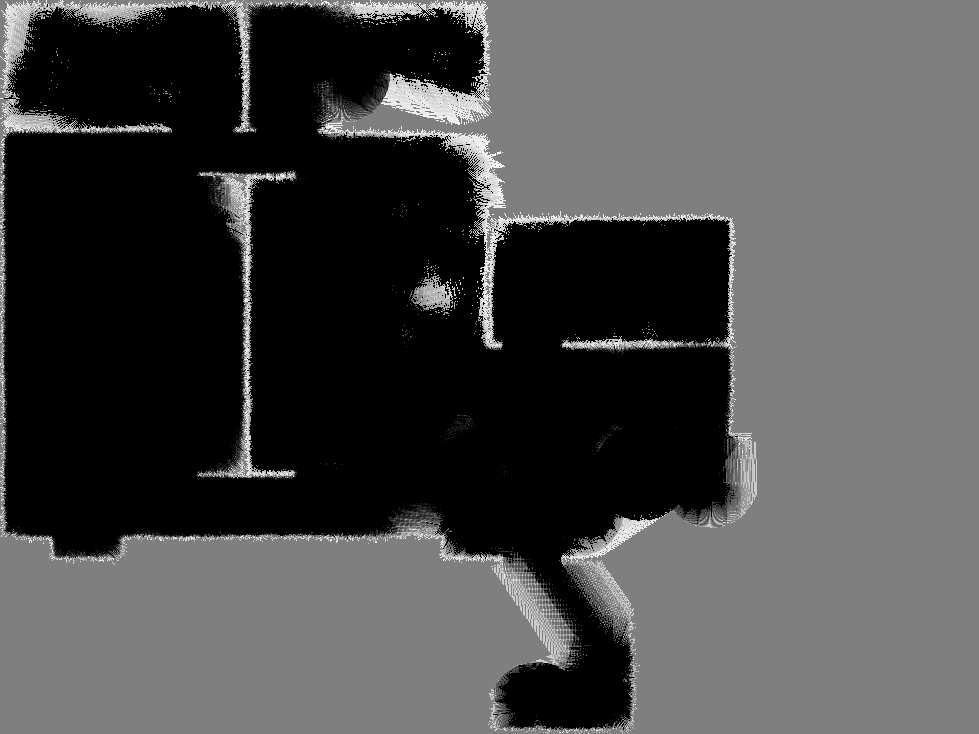
Fig. 13: Map of the autonomy laboratory environment (Figure 4(d)) generated by robots performing a SLW.

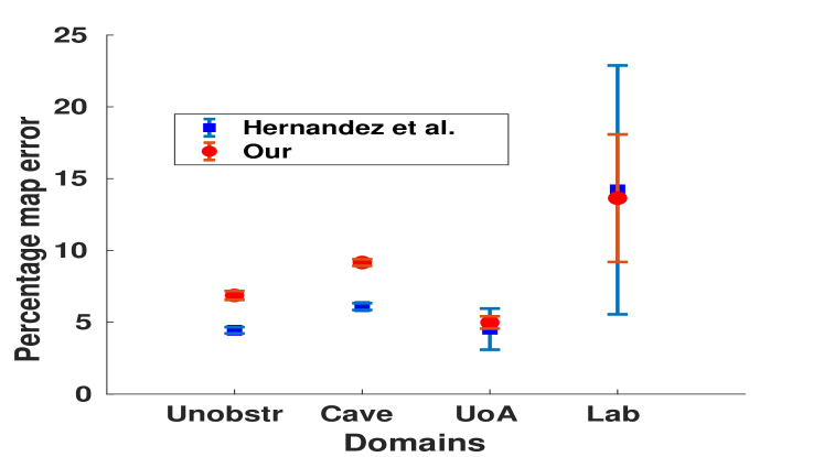
Fig. 14: Comparison of our strategy with the multi-robot mapping strategy in Hernández et al. [55]. The comparison is performed for the environments in Figure 4(a), Figure 4(b), Figure 4(c), and Figure 4(d). For each environment, the dot and square represent the median of the maximum error in the maps produced by our strategy and by the one in [55], respectively, over 10 simulation trials. The corresponding error bars indicate the largest and smallest maximum errors over the trials.

(a)

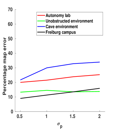
(b)

Fig. 15: (a) Time evolution of the mean minimum percentage of the unobstructed environment (Figure 4(a)) covered by the robots for different $\alpha$ values. (b) The mean maximum percent error in the maps for different robot localization uncertainties ($\sigma_{p}$) in four environments.

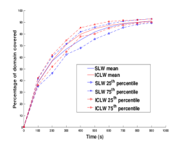
(a) Unobstructed environment

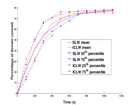
(b) Cave environment

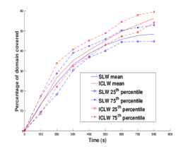
(c) Autonomy laboratory

Fig. 16: Time evolution of the percentage of the domain area covered by the robots during the same simulations as in Figure 12. The plot legends are the same as in Figure 12.

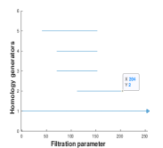
(a) $H_{0}$, Cave environment

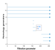
(b) $H_{1}$, Cave environment

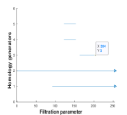
(c) $H_{0}$, Autonomy lab

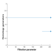
(d) $H_{1}$, Autonomy lab

Fig. 17: Barcode diagrams of the occupancy grid maps in Figure 5(b) (Figure 17(a), Figure 17(b)) and Figure 5(d) (Figure 17(c), Figure 17(d)). The filtration parameter $\varpi$ along the $x$-axes represents the pixel intensity of grid cells $m^{i}_{j}$ in the map, defined as the values of $\mathbb{P}_{m^{i}_{j}}$ scaled between 0 and 255. The filtration parameter ranges from 0 to 250. The $y$-axes show the number of homology generators for dimensions zero (Figure 17(a), Figure 17(c)) and one (Figure 17(b), Figure 17(d)).

VI SIMULATION RESULTS

In this section, we validate our distributed mapping technique with kinematic robots in five simulated environments with different sizes, shapes, and layouts, shown in Figure 4, using the robot simulator Stage [22]. The robots are controlled with velocity commands and have a maximum speed of $40$ cm/s, and they are equipped with on-board laser range sensors with a maximum range of $2$ m and a field-of-view of $180^{\circ}$. Each robot can communicate with any robot located within a circle of radius $2$ m. We set $p_{f}=0.1$, $p_{a}=0.5$, and $p_{hit}=0.9$ in Equation 11 and Equation 12. In order for the robots to perform the information correlated Lévy walk in the superdiffusive regime, the Lévy exponent $\alpha$ was set to $1.5$.

For each environment in Figure 4, we simulated a swarm of $N_{R}$ robots that explored the domain for $t_{f}$ seconds. Figure 5 shows the occupancy grid map that was generated by an arbitrary robot in the swarm after this amount of time. It is evident that each occupancy grid map is a reasonably accurate estimate of the corresponding environment in Figure 4. Although in this work, the robots stop exploring the domain and sharing their maps after a predefined time ($t_{f}$ seconds), they could alternatively be programmed to autonomously halt the mapping procedure once their stored occupancy grid maps stop changing significantly when they acquire new range measurements or maps communicated by neighboring robots.

Using a simulation of $N_{R}=5$ robots exploring the cave environment (Figure 4(b)) as an example, we illustrate the evolution of a robot’s occupancy map over time as it updates the map with new laser range sensor measurements and with the maps communicated by its neighbors. Figure 6 shows a sequence of snapshots of a simulation for this environment. The occupancy grid maps that are constructed by one of the robots in the swarm at the corresponding times are displayed in Figure 7. Note that the choice of the robots’ initial positions is arbitrary; the robots could ultimately produce a map of the environment starting from any initial positions, due to the diffusive nature of their exploratory random walks. Figure 8 depicts a collision avoidance maneuver performed by the robot in the green circle: upon encountering an obstacle, the robot follows a new heading that it computes from Equation 5. The accompanying multimedia attachment shows the video of this simulation with the occupancy grid maps of two robots evolving over time as the simulation progresses. The video demonstrates that the robots combine their individual maps when they are close enough to communicate, and that their maps eventually converge to a common occupancy map.

We quantified the degree of consensus on the occupancy map and the coverage performance of the swarm for simulations of the campus environment in Figure 4(e). After running a simulation with $N_{R}=50$ robots, we represented the set of occupancy probabilities $\mathbf{\bar{P}}_{M^{i}}$ computed by each robot $R^{i}$ at time $t_{f}=3600$ s as a matrix $\mathbf{P}_{M^{i}}$ with the dimensions of the occupancy grid map $M^{i}$. Figure 9 plots the normalized 2-norm $\|\mathbf{P}_{M^{i}}\|_{2}/\max_{i}\|\mathbf{P}_{M^{i}}\|_{2}$, $i=1,...,50$, which consolidates each robot’s set of occupancy probabilities into a single metric for comparison. The figure shows that the value of this metric has low variability across the robots, ranging at most $\sim 1.25\%$ from the maximum value for all but two robots. The occupancy grid maps of eight of the robots at time $t_{f}=3600$ s are shown in Figure 11. The similarity among the eight maps indicates that consensus has been achieved. In addition, we investigated the effect of the swarm size on coverage performance by simulating swarms of $N_{R}=$ 10, 20, 30, 40, and 50 robots for $t_{f}=3600$ s, running 10 simulations for each value of $N_{R}$. Figure 10 plots the percentage of the domain area that was covered by the robots after 3600 s for each swarm size $N_{R}$. The percentage of the domain covered is defined as the percentage of the total number of grid cells in the domain, including cells that overlap obstacles, for which the robots have obtained distance measurements. Each red dot marks the median percent coverage over 10 simulations, and the lower and upper error bars represent the $25^{th}$ and $75^{th}$ percentiles, respectively. The figure shows that for the same exploration time $t_{f}$, the percent coverage rises with increasing swarm size and saturates to approximately $40\%$ at around $N_{R}=40$. This relatively low percent coverage is due to the fact that in the campus environment, the robots cannot traverse the buildings, which function as obstacles; the percentage of the total number of grid cells that are accessible to the robots is about $40\%$.

We also compared our information correlated Lévy walk (ICLW) robot exploration strategy to a standard Lévy walk (SLW) strategy in terms of the entropy of the occupancy grid maps, defined in Equation 1, and the percent coverage of the domain. Figure 12 plots the time evolution of the resulting occupancy grid maps’ entropy for three simulated environments that robots explored using both SLW and ICLW strategies. For every environment, 30 simulations were run for each exploration strategy. Figure 13 shows the map of the autonomy laboratory environment (Figure 4(d)) that was generated by robots using the SLW exploration strategy, for comparison to the map obtained using the ICLW strategy in Figure 5(d). Figure 16 plots the time evolution of the percentage of each environment that was covered by the robots during the same simulations.

Figure 12 and Figure 16 show that when the robots perform the ICLW in the autonomy laboratory environment, the occupancy map entropy decreases more quickly and the percent coverage increases more quickly than when they perform the SLW. For the unobstructed and cave environments, the figures show that both the ICLW and SLW exploration strategies yield similar performance in terms of map entropy and percent coverage over time. Recall that these two environments, each with area 256 m², are significantly smaller than the 1200 m² autonomy laboratory. Since these environments are relatively small, the robots that explore them have a high rate of encounters with other robots and with the boundaries of the free space, which produces frequent changes in the robots’ headings. This causes the distribution of robot headings in these environments to more closely resemble a uniform distribution, as in the SLW.

Additionally, we compared our strategy with the multi-robot mapping strategy presented in Hernández et al. [55]. Like our strategy, the one in [55] uses multiple robots to generate occupancy grid maps; unlike ours, it is not an identity-free strategy. For both strategies, we ran 10 simulations on each of four environments shown in Figure 4 with the same parameters used to generate the maps in Figure 5. In each simulation, we obtained maps from all the robots exploring the domain. We selected the robot map with the maximum error, defined as the percent absolute error between the actual map and the robot-generated map. Figure 14 plots the median of the maximum errors obtained from the simulations, with error bars indicating the largest and smallest maximum errors over the trials. The results show that the performance of our strategy, in terms of the median of the maximum error, is comparable with that of the strategy presented in [55]. Our strategy produces a slightly higher median error for the unobstructed (Figure 4(a)) and cave (Figure 4(b)) environments, but yields a smaller range of error for the University of Auckland (UoA) robotics laboratory (Figure 4(c)) and autonomy laboratory (Figure 4(d)) environments.

To investigate the effect of the Lévy exponent $\alpha$ on the robots’ coverage of the domain, we performed simulations of $N_{R}=10$ robots exploring the unobstructed environment for $t_{f}=800$ seconds with $\alpha\in\{1.0,1.5,2.0,2.5,3.0\}$, running $10$ simulations for each value of $\alpha$. For each $\alpha$ value, Figure 15(a) plots the time evolution of the minimum percentage of the domain covered by the 10 robots, averaged over the 10 simulations for that $\alpha$ value. Interestingly, Figure 15(a) shows that there is not a significant effect of $\alpha$ on coverage of this environment for $1\leq\alpha\leq 3$. (A detailed investigation of the invariance of coverage to $\alpha$ in this range is beyond the scope of this paper.)

Furthermore, to test the robustness of our mapping strategy to uncertainty in robot localization, we conducted simulations in which we added zero-mean Gaussian noise with standard deviation $\sigma_{p}$ to the $x$ and $y$ coordinates of the robots’ positions. For each value $\sigma_{p}\in\{0.5,1.0,1.5,2.0\}$ meters, we ran 10 simulations on each of four environments shown in Figure 4 with the same parameters used to generate the maps in Figure 5. In each simulation, we obtained maps from all the robots exploring the domain. We selected the robot map with the maximum error, defined as the percent absolute error between the actual map and the robot-generated map. Figure 15(b) plots the mean of the maximum errors obtained from the simulations. The unobstructed environment is least affected by the noise, since it does not contain any obstacles. For the other environments, the mapping error increases with an increase in standard deviation, as expected. Observing the blue line (cave environment) in the plot, we find that the highest mapping error is only about $35\%$, even though the 2-meter standard deviation in the robot position is a substantial fraction of the environment dimensions (16 m $\times$ 16 m).

Finally, we tested our TDA-based adaptive thresholding technique on the occupancy grid maps in Figure 5(b) and Figure 5(d), which were generated for the cave and autonomy laboratory environments, respectively. The resulting barcode diagrams are shown in Figure 17. A topological feature is considered to be persistent if its corresponding arrow in the barcode diagram spans the entire range of the filtration parameter, $\varpi\in[0,250]$. The single arrow in Figure 17(a) and the four arrows that span $\varpi\in[0,250]$ in Figure 17(b) correctly indicate that Figure 5(b) has one connected component and four obstacles (topological holes), respectively. Similarly, the single arrows that span $\varpi\in[0,250]$ in Figure 17(c) and Figure 17(d) correctly indicate that Figure 5(d) has one connected component and one obstacle, respectively. In Figure 17(a) and Figure 17(b), the maximum filtration value for which all non-arrow line segments (which represent non-persistent topological features) terminate is $\varpi=204$, meaning that grid cells with pixel intensity greater than $204$ should be considered occupied. Therefore, any grid cell $m^{i}_{j}$ with an occupancy probability $\mathbb{P}_{m^{i}_{j}}\geq(204/255)=0.8$ is designated as an occupied cell. We arrive at a similar conclusion from Figure 17(c) and Figure 17(d).

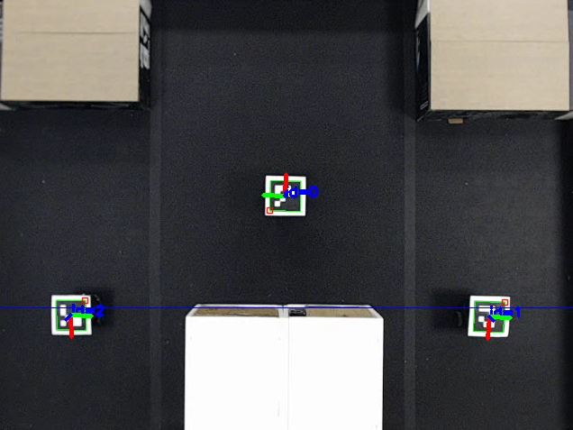
(a) Physical environment

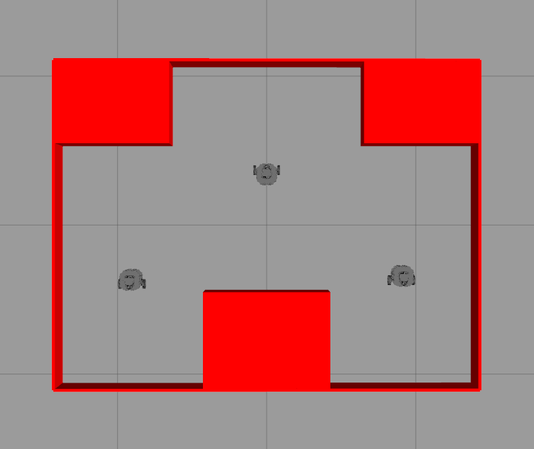
(b) Gazebo environment

Fig. 18: Overhead view of the physical experimental arena and Gazebo simulation arena with three rectangular obstacles and three robots in their initial positions for each trial.

VII ROBOT EXPERIMENTS

We also validated our mapping approach with physical experiments using small differential-drive robots. In this section, we describe the robot testbed, software framework, and experimental results.

VII-A Experimental Setup

Three Turtlebot3 Burger robots were used to conduct the experiments. The robots maneuver by means of two Dynamixel XL430-W250 actuators in a differential-drive configuration. Each robot is equipped with a Raspberry Pi 3 computer for high-level computation, such as image processing, networking, and controlling a 360^∘ Lidar sensor. Additionally, each robot has an OpenCR controller board with a microcontroller and various sensors. For high-level control, each robot’s Raspberry Pi runs the Dashing Diademata version of ros2, the next generation of the Robot Operating System (ROS) middleware, on Ubuntu 18.04 IoT Server. The robots have a communication range of 40 cm.

The experiments were conducted in a 2.78 m $\times$ 2.14 m arena containing three rectangular obstacles of different sizes, shown in Figure 18. All obstacles and the bordering walls of the arena had the same height, which was chosen to be high enough for the robots to detect these features with their Lidar sensors. An ArUco fiducial marker was fixed to the top of each robot, outside the range of the Lidar sensor, with a 3D-printed mount. To track the ArUco markers during the experiments, a Microsoft LifeCam camera was mounted to the ceiling over the arena and connected to a central computer. It should be noted that the size of the arena was limited by the ceiling height, which restricted the camera’s field-of-view. In addition, camera option restrictions imposed by the OS (Ubuntu) on the central computer limited the resolution of the camera image.

The code used in the simulations in Section VI was modified for implementation on the robots. As in the simulations, we set $p_{f}=0.1$, $p_{a}=0.5$, and $p_{hit}=0.9$ in Equation 11 and Equation 12, and the Lévy exponent $\alpha$ was set to $1.5$. To account for the relatively small size of the arena, each robot’s Lidar sensor range was limited to a maximum distance of 40 cm and a field-of-view of 180^∘ instead of the default 2 m maximum distance and 360^∘ field-of-view.

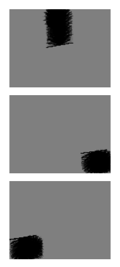
(a) Maps at 0.5 min (exp)

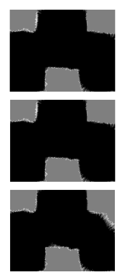
(b) Maps at 10 min (exp)

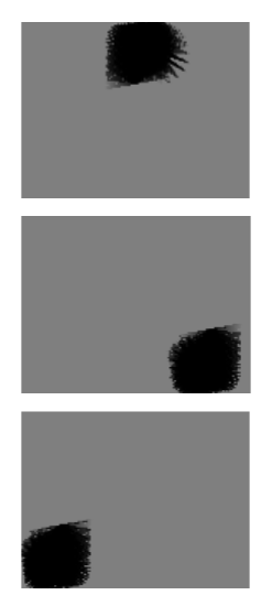
(c) Maps at 0.5 min (sim)

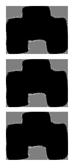
(d) Maps at 10 min (sim)

Fig. 19: Occupancy grid maps generated by robot $R^{0}$ (top row), robot $R^{1}$ (middle row), and robot $R^{2}$ (bottom row) at 0.5 min and 10 min during an experimental trial (left two columns) and a Gazebo simulation trial (right two columns). Robot labels are shown in Figure 18, detected by the overhead camera from the ArUco markers.

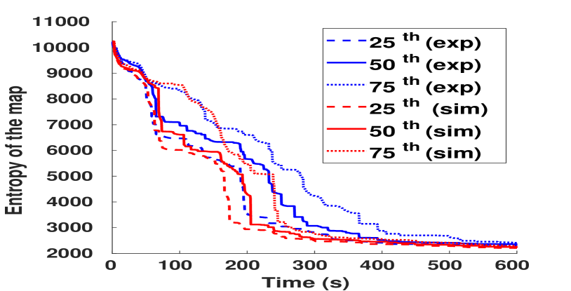
(a) Entropy of occupancy maps

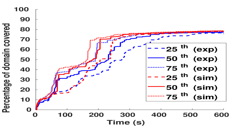
(b) Percentage coverage

Fig. 20: Time evolution during 10 experimental (blue) and simulation (red) trials of (a) the entropy $H(M^{i})$ of occupancy maps $M^{i}$, $i=1,2,3$, and (b) the percentage of the domain area covered by the robots. The plots show the $25^{th}$ percentile (dashed line), $50^{th}$ percentile (solid line), and $75^{th}$ percentile (dotted line) of these quantities from the 10 trials.

VII-B Software Architecture

By using ros2, we were able to distribute much of the computing necessary for the experiments. To do this, ros2 utilizes the concept of nodes, which contain code for executing specific tasks. For example, sensor information from a robot’s Lidar is processed and used to construct the robot’s occupancy grid map in a node. The information generated in this node can then be sent to other nodes. For our experiments, we distributed nodes across the three robots and a central computer. The robots were all given the same nodes, but were assigned unique identifiers to individualize their information.

Compared to the original ROS, ros2 does not have a ROS Master which connects nodes that are distributed across multiple machines. Instead, each component within the system communicates using a Data Distribution Service (DDS), making the system decentralized and improving its robustness to failure. If any robot or the central computer were to fail, the remaining components will continue to work until the failing component is returned to an operational status. In this work, the central computer ran nodes that acquire information from the overhead camera and disseminate the information to the robots. The overhead camera node calculated the position and orientation of each robot from its ArUco marker. The robots require this information to build their occupancy grid maps and to identify robots that are within their communication range for sharing maps.

Each robot ran three nodes: one to transmit information to and from the OpenCR controller board, a second to collect and publish information from the Lidar sensor, and a third to provide the high-level control pertaining to the Lévy walk exploration strategy. All robots communicated with the central computer and with each other using the on-board WiFi modules on the Raspberry Pi 3.

VII-C Experimental Results

Ten experimental trials were run for 10 minutes each. To minimize robot interactions early on in the experiments, the robots were placed in different parts of the arena in the same locations at the beginning of each trial (see Figure 18). During every trial, each robot generated an occupancy grid map and computed its occupancy map entropy and percent coverage of the domain every 0.1 s. To conserve memory on the robot, however, the occupancy grid map image was saved only every 30 s. In addition to the physical experiments, ten Gazebo [56] simulations were run with the same parameters as the experiments in a reproduction of the experimental testbed, shown in Figure 18(b). These simulations provide a basis of comparison for the performance of our approach in a noise- and error-free environment.

Figure 19 shows the occupancy grid maps of each robot at 0.5 min and 10 min for an experimental trial and a simulation trial. The maps at the end of the trial (10 min) approximate the actual environment, and the similarity of these maps indicates that the robots have reached consensus. The accompanying multimedia attachment shows the video of the experimental trial with the time evolution of the robots’ occupancy grid maps over the entire trial. Figure 20(a) and Figure 20(b) plot the time evolution of the occupancy grid maps’ entropy and the percent coverage of the domain, respectively, over all trials. From Figure 20(a), we see that the entropy of the occupancy maps is minimized within about $500$ s in all trials, indicating that the robots have achieved consensus on a map of the domain with minimum uncertainty. Moreover, Figure 20(b) shows that the percentage of the domain covered by the robots reaches its maximum value around this time in all trials. The figure shows that the results from the ten Gazebo simulations are comparable to the results from the physical experiments, and their entropy and percent coverage values converge to nearly the same value at the final time. This similarity suggests that our approach is robust to noise and errors that occur in physical environments.

VIII Conclusion

In this work, we developed a novel distributed approach to generating an occupancy grid map of an unknown environment using a swarm of robots with local communication. The approach is scalable with the number of robots and robust to robot errors and failures. We also presented a robot exploration strategy, referred to as an information correlated Lévy walk, that directs Lévy-walking robots to regions that maximize the their information gain. In addition, we demonstrated that a technique based on topological data analysis, which we used in our earlier works to construct topological maps of unknown environments, can also be used for adaptive thresholding of occupancy grid maps. We validated our mapping methodology through simulations and physical robot experiments on domains with different geometries and sizes.

One direction for future work is to extend our mapping approach to the case where the robots have no global localization or are only capable of weak localization, which we define as pose estimation with bounded uncertainty, using a received signal strength indicator (RSSI) device [57] or ultra-wideband (UWB) sensors [58, 59]. This will allow our approach to be applied in GPS-denied environments. Another future objective is to derive the partial differential equation model that describes the spatiotemporal evolution of the swarm population dynamics as the robots perform information correlated Lévy walks. This will enable an analytical investigation of the performance of our exploration strategy.

Appendix A Derivation of formula to compute $\mathbf{I}[\mathbf{c}^{i,a}_{\tau};z^{i,a}_{\tau}]$

By definition,

$$\mathbf{I}[\mathbf{c}^{i,a}_{\tau};z^{i,a}_{\tau}]=\int_{z\in z^{i,a}_{\tau}}\sum_{c\in\mathbf{c}^{i,a}_{\tau}}\mathbb{P}(c,z)\log_{2}\left(\frac{\mathbb{P}(c,z)}{\mathbb{P}(c)\mathbb{P}(z)}\right)dz$$

This expression can be rewritten as,

$$\mathbf{I}[\mathbf{c}^{i,a}_{\tau};z^{i,a}_{\tau}] {}={} \int_{z\in z^{i,a}_{\tau}}\sum_{c\in\mathbf{c}^{i,a}_{\tau}}\mathbb{P}(c,z)\log_{2}\left(\mathbb{P}(z,c)\right)dz$$

$${-}\>\int_{z\in z^{i,a}_{\tau}}\sum_{c\in\mathbf{c}^{i,a}_{\tau}}\mathbb{P}(c,z)\log_{2}\left(\mathbb{P}(z)\mathbb{P}(c)\right)dz$$

Define

$$\mathbf{P1}=\int_{z\in z^{i,a}_{\tau}}\sum_{c\in\mathbf{c}^{i,a}_{\tau}}\mathbb{P}(c,z)\log_{2}\left(\mathbb{P}(z,c)\right)dz$$

and

$$\mathbf{P2}=\int_{z\in z^{i,a}_{\tau}}\sum_{c\in\mathbf{c}^{i,a}_{\tau}}\mathbb{P}(c,z)\log_{2}\left(\mathbb{P}(z)\mathbb{P}(c)\right)dz$$

Expanding $\mathbf{P1}$ yields,

$$\mathbf{P1} {}={} \int_{z\in z^{i,a}_{\tau}}\sum_{p=0}^{|\mathbf{c}^{i,a}_{\tau}|}(\mathbb{P}(z|e_{p})\mathbb{P}(e_{p})\log_{2}\left(\mathbb{P}(z|e_{p})\right)$$

$$~{}~{}~{}~{}~{}~{}~{}~{}~{}~{}~{}~{}{+}~{}\>\mathbb{P}(z|e_{p})\mathbb{P}(e_{p})\log_{2}\left(\mathbb{P}(e_{p})\right))dz$$

Rearranging this expression, we obtain

$$\mathbf{P1} {}={} \sum_{p=0}^{|\mathbf{c}^{i,a}_{\tau}|}\mathbb{P}(e_{p})\int_{z\in z^{i,a}_{\tau}}\mathbb{P}(z|e_{p})\log_{2}(\mathbb{P}(z|e_{p}))dz$$

$${+}\>\sum_{p=0}^{|\mathbf{c}^{i,a}_{\tau}|}\mathbb{P}(e_{p})\log_{2}(\mathbb{P}(e_{p}))\int_{z\in z^{i,a}_{\tau}}\mathbb{P}(z|e_{p})dz$$

Using the fact that $\int_{z\in z^{i,a}_{\tau}}\mathbb{P}(z|e_{p})dz=1$ and substituting $\mathbb{P}(z|e_{k})$, defined as the Gaussian forward measurement model in Equation 3, into the above equation, we find the following expression for $\mathbf{P1}$ after simplification:

$$\mathbf{P1}=-\log_{2}(\sqrt{2\pi}\sigma)-0.5+\sum_{p=0}^{|\mathbf{c}^{i,a}_{\tau}|}\mathbb{P}(e_{p})\log_{2}(\mathbb{P}(e_{p}))$$

The expression for $\mathbf{P2}$ can be split into the sum of the following two terms, which we denote as $\mathbf{P2}_{a}$ and $\mathbf{P2}_{b}$, respectively:

$$\mathbf{P2} {}={} \int_{z\in z^{i,a}_{\tau}}\sum_{c\in\mathbf{c}^{i,a}_{\tau}}\mathbb{P}(c,z)\log_{2}(\mathbb{P}(c))dz$$

$${+}\>\int_{z\in z^{i,a}_{\tau}}\sum_{c\in\mathbf{c}^{i,a}_{\tau}}\mathbb{P}(c,z)\log_{2}(\mathbb{P}(z))dz$$

$\mathbf{P2}_{a}$ can be expanded as,

$$\mathbf{P2}_{a}=\int_{z\in z^{i,a}_{\tau}}\sum_{p=0}^{|\mathbf{c}^{i,a}_{\tau}|}\mathbb{P}(z|e_{p})\mathbb{P}(e_{p})\log_{2}(\mathbb{P}(e_{p}))dz$$

$$=\sum_{p=0}^{|\mathbf{c}^{i,a}_{\tau}|}\mathbb{P}(e_{p})\log_{2}(\mathbb{P}(e_{p}))\int_{z\in z^{i,a}_{\tau}}\mathbb{P}(z|e_{p})dz$$

Since $\sum_{c\in\mathbf{c}^{i,a}_{\tau}}\mathbb{P}(c,z)$ reduces to $\mathbb{P}(z)$ (by marginalization over $c$), $\mathbf{P2}_{b}$ can be expressed as,

$$\mathbf{P2}_{b}=\int_{z\in z^{i,a}_{\tau}}\mathbb{P}(z)\log_{2}(\mathbb{P}(z))dz$$

Finally, using our derived equations for $\mathbf{P1}$, $\mathbf{P2}$ and the fact that $\int_{z\in z^{i,a}_{\tau}}\mathbb{P}(z|e_{p})dz=1$, we obtain the following formula:

$$\mathbf{I}[\mathbf{c}^{i,a}_{\tau};z^{i,a}_{\tau}]=-\int_{z\in z^{i,a}_{\tau}}\mathbb{P}(z)\log_{2}(\mathbb{P}(z))dz-\log_{2}(\sqrt{2\pi}\sigma)-0.5$$

∎

Appendix B Proof of Theorem 1

Proof.

We abbreviate $u(m^{i}_{j},\mathbf{x}^{i}_{k},\mathbf{z}^{i}_{k})$ as $u^{i}_{j}(k)$ and define $\mathbb{L}x=-\log_{2}(x)$ for $x>0$. Taking the negative logarithm of both sides of Equation 13, we obtain:

$$\mathbb{L}\mathbb{P}_{m^{i}_{j}}(k+1)=\sum_{\hat{n}\in\mathbb{N}^{i}_{k}\cup i}a_{i\hat{n}}(k)\left(\mathbb{L}\mathbb{P}_{m^{\hat{n}}_{j}}(k)\right)+\mathbb{L}u^{i}_{j}(k)$$ (17)

Let $\mathbb{L}\mathbb{P}_{m_{j}}[k]=[\mathbb{L}\mathbb{P}_{m^{1}_{j}}(k)~{}...~{}\mathbb{L}\mathbb{P}_{m^{N_{R}}_{j}}(k)]^{T}$ and $\mathbb{L}\mathbf{u}_{j}[k]=[\mathbb{L}u^{1}_{j}(k)~{}...~{}\mathbb{L}u^{N_{R}}_{j}(k)]^{T}$. Then Equation 17 can be written in the following form:

$$\mathbb{L}\mathbb{P}_{m_{j}}[k+1]~{}=~{}\mathbb{A}[k]\left(\mathbb{L}\mathbb{P}_{m_{j}}[k]\right)+\mathbb{L}\mathbf{u}_{j}[k],$$ (18)

where $\mathbb{A}[k]$ is the adjacency matrix of the time-varying robot communication graph $\mathbb{G}(k)$, as defined in Section IV-B.

Given an initial time step $k_{0}\geq 0$, we define $\Phi_{\mathbb{A}}[k,k_{0}]=\mathbb{A}[k]\mathbb{A}[k-1]\cdots\mathbb{A}[k_{0}]$. Then the information dynamics described in Equation 18 can be expanded as:

$$\mathbb{L}\mathbb{P}_{m_{j}}[k+1]=\Phi_{\mathbb{A}}[k,0](\mathbb{L}\mathbb{P}_{m_{j}}[0])+\sum_{d\in\mathbf{d}}\Phi_{\mathbb{A}}[k,d](\mathbb{L}{\mathbf{u}_{j}[k]})$$ (19)

If Assumption 1 holds and $\mathbb{A}[k]$ is a doubly stochastic matrix for each $k$, then by [14, Theorem 1], we have that

$$\lim_{k\rightarrow\infty}\Phi_{\mathbb{A}}[k,k_{0}]=\frac{1}{N_{R}}\mathbf{1}\mathbf{1}^{T},$$

where $\mathbf{1}\in\mathbb{R}^{N_{R}}$ is a column vector of ones. By [60, Theorem 11.6], $\Phi_{\mathbb{A}}[k,k_{0}]$ converges exponentially to $\frac{1}{N_{R}}\mathbf{1}\mathbf{1}^{T}$. Assumption 2 ensures that $\mathbb{A}[k]$ is doubly stochastic for all $k$. Taking the limit of Equation 19 as $k\rightarrow\infty$ and using the above result yields,

$$\lim_{k\rightarrow\infty}\mathbb{L}\mathbb{P}_{m_{j}}[k] {}={} \mathbf{1}\left(\frac{1}{N_{R}}\mathbf{1}^{T}(\mathbb{L}\mathbb{P}_{m_{j}}[0])\right)$$

$${+}~{}\>\mathbf{1}\left(\sum_{d\in\mathbf{d}}\frac{1}{N_{R}}\mathbf{1}^{T}(\mathbb{L}{\mathbf{u}_{j}[k]})\right)$$

The product of $\frac{1}{N_{R}}\mathbf{1}^{T}$ and a column vector with $N_{R}$ non-negative elements is equal to the arithmetic mean of the elements of the vector. Denoting $<\cdot>$ as the arithmetic mean operator, we can therefore rewrite the above equation as:

$$\lim_{k\rightarrow\infty}\mathbb{L}\mathbb{P}_{m_{j}}[k]~{}=~{}\mathbf{1}\left\langle\mathbb{L}\mathbb{P}_{m_{j}}[0]\right\rangle+\mathbf{1}\sum_{d\in\mathbf{d}}\left\langle\mathbb{L}\mathbf{u}_{j}[k]\right\rangle$$ (20)

Assumption 3 is required to ensure the convergence of the sum $\sum_{d\in\mathbf{d}}\left\langle\mathbb{L}{\mathbf{u}_{j}[k]}\right\rangle$.

By Equation 20, the limit of the $i^{th}$ element of $\mathbb{L}\mathbb{P}_{m_{j}}[k]$ as $k\rightarrow\infty$ is given by:

$$\lim_{k\rightarrow\infty}\mathbb{L}\mathbb{P}_{m^{i}_{j}}(k)~{}=~{}\left\langle\mathbb{L}\mathbb{P}_{m_{j}}[0]\right\rangle+\sum_{d\in\mathbf{d}}\left\langle\mathbb{L}{\mathbf{u}_{j}[d]}\right\rangle$$

Since $\mathbf{d}$ is a finite set and $\Phi_{\mathbb{A}}[k,k_{0}]$ converges exponentially to $\frac{1}{N_{R}}\mathbf{1}\mathbf{1}^{T}$, the above equation converges exponentially.

Finally, by taking the exponential of both sides of the above equation, we obtain the desired result (Equation 14):

$$\lim_{k\rightarrow\infty}\mathbb{P}_{m^{i}_{j}}(k)~{}=~{}<\mathbb{P}_{m_{j}}[0]>_{gm}\hskip 2.84526pt\cdot\hskip 2.84526pt\prod_{d\in\mathbf{d}}<\mathbf{u}_{j}[d]>_{gm}$$

For inaccessible grid cells $m^{i}_{a}$, $\mathbf{u}_{a}[d]=\mathbf{1}$ for all $d$ since none of the robots’ measurements provide any information about the occupancy probability of these cells. Therefore, Equation 14 reduces to

$$\lim_{k\rightarrow\infty}\mathbb{P}_{m^{i}_{\bar{a}}}(k)~{}=~{}<\mathbb{P}_{m_{\bar{a}}}[0]>_{gm}.$$ (21)

Now we consider the set of accessible grid cells. Let the elements of the set $\mathbf{d}$ be denoted by $d_{1},d_{2},\cdots,d_{\gamma}$, where $\gamma$ is the cardinality of $\mathbf{d}$. Then,

$$\prod_{d\in\mathbf{d}}<\mathbf{u}_{a}[d]>_{gm}=$$

$$<\mathbf{u}_{a}[d_{1}]>_{gm}~{}~{}\cdot <\mathbf{u}_{a}[d_{2}]>_{gm}~{}~{}\cdots~{}~{}<\mathbf{u}_{a}[d_{\gamma}]>_{gm}$$

Using the definition of geometric mean, the above equation can be written as,

$$\prod_{d\in\mathbf{d}}<\mathbf{u}_{a}[d]>_{gm}=\sqrt[N_{R}]{\prod_{q=1}^{N_{R}}\mathbf{u}_{a}[d_{1}](q)\cdots\prod_{q=1}^{N_{R}}\mathbf{u}_{a}[d_{\gamma}](q)}~{},$$

where $\mathbf{u}_{a}[d_{1}](q)$ is the $q^{th}$ element of the vector $\mathbf{u}_{a}[d_{1}]$. The right-hand side of the above equation contains a product of $N_{R}\gamma$ positive real numbers. Since under Assumption 3A, all elements of this product are equal to one except for the $N_{R}$ values $\bar{u}_{a}^{1},...,\bar{u}_{a}^{N_{R}}$, the above equation can be reduced to

$$\prod_{d\in\mathbf{d}}<\mathbf{u}_{a}[d]>_{gm}~{}=~{}\sqrt[N_{R}]{\bar{u}^{1}_{a}\cdot\bar{u}^{2}_{a}~{}\cdots~{}\bar{u}^{N_{R}}_{a}}.$$

Therefore,

$$\prod_{d\in\mathbf{d}}<\mathbf{u}_{a}[d]>_{gm}~{}=~{}<[\bar{u}^{1}_{a}~{}\cdots~{}\bar{u}^{N_{R}}_{a}]^{T}>_{gm}.$$

Combining the above result with Equation 14 yields,

$$\lim_{k\rightarrow\infty}\mathbb{P}_{m^{i}_{a}}(k)~{}=~{}<\mathbb{P}_{m_{a}}[0]>_{gm}\hskip 2.84526pt\cdot\hskip 2.84526pt<[\bar{u}^{1}_{a}~{}\cdots~{}\bar{u}^{N_{R}}_{a}]^{T}>_{gm}.$$

∎

Ragesh Kumar Ramachandran received the B.Tech degree in civil engineering from National Institute of Technology Calicut, India, in 2011, and the M.S. and Ph.D. degrees in mechanical engineering from Arizona State University, Tempe, AZ, USA, in 2018. Since 2018, he has been a postdoctoral researcher in computer science at the University of Southern California. His current research interests include the design and analysis of algorithms for solving problems in robotic swarms and multi-robot systems, network and graph theory, optimal and nonlinear control theory, and applied topology and differential geometry.

Zahi Kakish received the B.S. degree in mechanical polymer engineering from the University of Akron, Akron, OH, in 2013. He received the M.S. degree in mechanical engineering from the University of Akron in 2015. Currently, he is a Ph.D. student in mechanical engineering at Arizona State University, where his research interests include swarm intelligence, human-swarm interaction, and multi-agent reinforcement learning.

Spring Berman (M’07) received the M.S.E. and Ph.D. degrees in mechanical engineering and applied mechanics from the University of Pennsylvania in 2008 and 2010, respectively. From 2010 to 2012, she was a postdoctoral researcher in computer science at Harvard University. Since 2012, she has been a professor of mechanical and aerospace engineering at Arizona State University. Her research focuses on the analysis of behaviors in biological and engineered collectives and the synthesis of control strategies for robotic swarms. She received the 2014 DARPA Young Faculty Award and the 2016 ONR Young Investigator Award.

References

- [1] S. Thrun, W. Burgard, and D. Fox, Probabilistic Robotics (Intelligent Robotics and Autonomous Agents). The MIT Press, 2005.
- [2] R. Smith, M. Self, and P. Cheeseman, “A stochastic map for uncertain spatial relationships,” in Proceedings of the 4th International Symposium on Robotics Research. Cambridge, MA, USA: MIT Press, 1988, pp. 467–474.
- [3] A. Elfes, “Using occupancy grids for mobile robot perception and navigation,” Computer, vol. 22, no. 6, pp. 46–57, June 1989.
- [4] H. Choset and K. Nagatani, “Topological simultaneous localization and mapping (SLAM): Toward exact localization without explicit localization,” IEEE Transactions on Robotics and Automation, vol. 17, pp. 125–137, 2001.
- [5] A. Howard, “Multi-robot simultaneous localization and mapping using particle filters,” The International Journal of Robotics Research, vol. 25, no. 12, pp. 1243–1256, 2006.
- [6] S. B. Williams, G. Dissanayake, and H. Durrant-Whyte, “Towards multi-vehicle simultaneous localisation and mapping,” in Proceedings of the IEEE International Conference on Robotics and Automation, vol. 3, 2002, pp. 2743–2748.
- [7] S. Saeedi, M. Trentini, M. Seto, and H. Li, “Multiple-robot simultaneous localization and mapping: A review,” Journal of Field Robotics, vol. 33, no. 1, pp. 3–46, Jan. 2016.
- [8] R. Aragues, J. Cortes, and C. Sagues, “Distributed consensus on robot networks for dynamically merging feature-based maps,” IEEE Transactions on Robotics, vol. 28, no. 4, pp. 840–854, Aug. 2012.
- [9] D. Gonzalez-Arjona, A. Sanchez, F. López-Colino, A. de Castro, and J. Garrido, “Simplified occupancy grid indoor mapping optimized for low-cost robots,” ISPRS International Journal of Geo-Information, vol. 2, no. 4, pp. 959–977, 2013.
- [10] S. Saeedi, L. Paull, M. Trentini, and H. Li, “Occupancy grid map merging for multiple robot simultaneous localization and mapping,” International Journal of Robotics and Automation, vol. 30, no. 2, pp. 149–157, 2015.
- [11] Z. Jiang, J. Zhu, Y. Li, J. Wang, Z. Li, and H. Lu, “Simultaneous merging multiple grid maps using the robust motion averaging,” Journal of Intelligent & Robotic Systems, pp. 1–14, Aug. 2018.
- [12] S. Carpin, “Fast and accurate map merging for multi-robot systems,” Autonomous Robots, vol. 25, no. 3, pp. 305–316, Oct. 2008.
- [13] P. D’Alberto and A. Nicolau, “Using recursion to boost atlas’s performance,” in High-Performance Computing. Springer, 2005, pp. 142–151.
- [14] D. B. Kingston and R. W. Beard, “Discrete-time average-consensus under switching network topologies,” in Proceedings of the American Control Conference, June 2006.
- [15] H. Mangesius, D. Xue, and S. Hirche, “Consensus driven by the geometric mean,” IEEE Transactions on Control of Network Systems, vol. 5, no. 1, pp. 251–261, 2018.
- [16] T. M. Cover and J. A. Thomas, Elements of Information Theory (Wiley Series in Telecommunications and Signal Processing). New York, NY, USA: Wiley-Interscience, 2006.
- [17] R. Fujisawa and S. Dobata, “Lévy walk enhances efficiency of group foraging in pheromone-communicating swarm robots,” in Proceedings of the IEEE/SICE International Symposium on System Integration, Dec. 2013, pp. 808–813.
- [18] R. K. Ramachandran, S. Wilson, and S. Berman, “A probabilistic approach to automated construction of topological maps using a stochastic robotic swarm,” IEEE Robotics and Automation Letters, vol. 2, no. 2, pp. 616–623, Apr. 2017.
- [19] A. Hatcher, Algebraic Topology. New York, NY: Cambridge University Press, 2002.
- [20] T. Kaczynski, K. Mischaikow, and M. Mrozek, Computational Homology. Springer-Verlag New York, 2004.
- [21] H. Edelsbrunner and J. L. Harer, “Persistent homology - a survey,” Contemporary Mathematics, vol. 453, pp. 257–282, 2008.
- [22] R. Vaughan, “Massively multi-robot simulation in stage,” Swarm Intelligence, vol. 2, no. 2, pp. 189–208, Dec. 2008.
- [23] R. K. Ramachandran, K. Elamvazhuthi, and S. Berman, “An optimal control approach to mapping GPS-denied environments using a stochastic robotic swarm,” in Robotics Research. Springer, 2018, pp. 477–493.
- [24] R. K. Ramachandran, S. Wilson, and S. Berman, “A probabilistic topological approach to feature identification using a stochastic robotic swarm,” in Distributed Autonomous Robotic Systems. Springer, 2018, pp. 3–16.
- [25] R. K. Ramachandran and S. Berman, “Automated construction of metric maps using a stochastic robotic swarm leveraging received signal strength,” in Proceedings of the 3rd International Symposium on Swarm Behavior and Bio-Inspired Robotics. SWARM, 2019, to appear.
- [26] LMS200/211/221/291 Laser Measurement Systems, SICK Sensor Intelligence, 2006.
- [27] M. Kegeleirs, D. G. Ramos, and M. Birattari, “Random walk exploration for swarm mapping,” Universit é Libre de Bruxelles, Tech. Rep. TR/IRIDIA/2019-001, 02 2019. [Online]. Available: http://iridia.ulb.ac.be/IridiaTrSeries/link/IridiaTr2019-001.pdf
- [28] G. M. Fricke, J. P. Hecker, J. L. Cannon, and M. E. Moses, “Immune-inspired search strategies for robot swarms,” Robotica, vol. 34, no. 8, pp. 1791–1810, 2016.
- [29] E. Gelenbe, N. Schmajuk, J. Staddon, and J. Reif, “Autonomous search by robots and animals: A survey,” Robotics and Autonomous Systems, vol. 22, no. 1, pp. 23 – 34, 1997, Biologically Inspired Autonomous Systems.
- [30] C. Dimidov, G. Oriolo, and V. Trianni, “Random walks in swarm robotics: An experiment with Kilobots,” in Swarm Intelligence, M. Dorigo, M. Birattari, X. Li, M. López-Ibáñez, K. Ohkura, C. Pinciroli, and T. Stützle, Eds. Cham: Springer International Publishing, 2016, pp. 185–196.
- [31] S. Wilson, T. P. Pavlic, G. P. Kumar, A. Buffin, S. C. Pratt, and S. Berman, “Design of ant-inspired stochastic control policies for collective transport by robotic swarms,” Swarm Intelligence, vol. 8, no. 4, pp. 303–327, Dec. 2014.
- [32] A. Dirafzoon, A. Bozkurt, and E. J. Lobaton, “Dynamic topological mapping with biobotic swarms,” CoRR, vol. abs/1507.03206, 2015.
- [33] D. Sutantyo, P. Levi, C. Möslinger, and M. Read, “Collective-adaptive Lévy flight for underwater multi-robot exploration,” in Proceedings of the IEEE International Conference on Mechatronics and Automation, 2013, pp. 456–462.
- [34] B. Pang, Y. Song, C. Zhang, H. Wang, and R. Yang, “A swarm robotic exploration strategy based on an improved random walk method,” Journal of Robotics, vol. 2019, 2019.
- [35] S. G. Nurzaman, Y. Matsumoto, Y. Nakamura, K. Shirai, S. Koizumi, and H. Ishiguro, “From Lévy to Brownian: a computational model based on biological fluctuation,” PLOS ONE, vol. 6, no. 2, p. e16168, 2011.
- [36] B. Charrow, S. Liu, V. Kumar, and N. Michael, “Information-theoretic mapping using Cauchy-Schwarz quadratic mutual information,” in Proceedings of the IEEE International Conference on Robotics and Automation, May 2015, pp. 4791–4798.
- [37] B. J. Julian, S. Karaman, and D. Rus, “On mutual information-based control of range sensing robots for mapping applications,” in Proceedings of the IEEE/RSJ International Conference on Intelligent Robots and Systems, Nov. 2013, pp. 5156–5163.
- [38] V. Zaburdaev, S. Denisov, and J. Klafter, “Lévy walks,” Reviews of Modern Physics, vol. 87, no. 2, p. 483, 2015.
- [39] B. J. Julian, “Mutual information-based gradient-ascent control for distributed robotics,” Ph.D. dissertation, Massachusetts Institute of Technology, 2013.
- [40] H. Kretzschmar and C. Stachniss, “Information-theoretic compression of pose graphs for laser-based SLAM,” The International Journal of Robotics Research, vol. 31, no. 11, pp. 1219–1230, Aug. 2012.
- [41] B. Charrow, G. Kahn, S. Patil, S. Liu, K. Goldberg, P. Abbeel, N. Michael, and V. Kumar, “Information-theoretic planning with trajectory optimization for dense 3D mapping,” in Proceedings of Robotics: Science and Systems, vol. 6, 2015.
- [42] S. Thrun, “Learning occupancy grid maps with forward sensor models,” Autonomous Robots, vol. 15, no. 2, pp. 111–127, Sept. 2003.
- [43] K. Pathak, A. Birk, J. Poppinga, and S. Schwertfeger, “3D forward sensor modeling and application to occupancy grid based sensor fusion,” in Proceedings of the IEEE/RSJ International Conference on Intelligent Robots and Systems, Oct. 2007, pp. 2059–2064.
- [44] R. Olfati-Saber and R. M. Murray, “Consensus problems in networks of agents with switching topology and time-delays,” IEEE Transactions on Automatic Control, vol. 49, no. 9, pp. 1520–1533, Sept. 2004.
- [45] W. Ren and R. W. Beard, “Consensus of information under dynamically changing interaction topologies,” in Proceedings of the American Control Conference, vol. 6, June 2004, pp. 4939–4944.
- [46] L. Moreau, “Stability of multiagent systems with time-dependent communication links,” IEEE Transactions on Automatic Control, vol. 50, no. 2, pp. 169–182, Feb. 2005.
- [47] C. Godsil and G. Royle, Algebraic Graph Theory, ser. Graduate Texts in Mathematics. New York: Springer-Verlag, 2001, vol. 207.
- [48] K. R. Das and A. R. Imon, “Geometric median and its application in the identification of multiple outliers,” Journal of Applied Statistics, vol. 41, no. 4, pp. 817–831, 2014.
- [49] H. Edelsbrunner and J. L. Harer, Computational Topology: An Introduction. Providence (R.I.): American Mathematical Society, 2010.
- [50] R. Ghrist, “Barcodes: the persistent topology of data,” Bulletin of the American Mathematical Society, vol. 45, no. 1, pp. 61–75, 2008.
- [51] G. Carlsson, “Topology and data,” Bulletin of the American Mathematical Society, vol. 46, no. 2, pp. 255–308, 2009.
- [52] S. M. LaValle, Planning Algorithms. New York, NY, USA: Cambridge University Press, 2006.
- [53] V. Nanda, “Perseus, the persistent homology software,” http://www.sas.upenn.edu/~vnanda/perseus, 2019.
- [54] R. Vaughan, “Stage,” https://github.com/rtv/Stage, 2019.
- [55] C. A. V. Hernández and F. A. P. Ortiz, “A real-time map merging strategy for robust collaborative reconstruction of unknown environments,” Expert Systems with Applications, vol. 145, p. 113109, 2020.
- [56] N. Koenig and A. Howard, “Design and use paradigms for Gazebo, an open-source multi-robot simulator,” in Proceedings of the IEEE/RSJ International Conference on Intelligent Robots and Systems (IROS), vol. 3, Sept. 2004, pp. 2149–2154.
- [57] Y. Xie, Z. Li, and M. Li, “Precise power delay profiling with commodity WiFi,” in Proceedings of the 21st Annual International Conference on Mobile Computing and Networking, ser. MobiCom ’15. New York, NY, USA: ACM, 2015, pp. 53–64.
- [58] A. Prorok and A. Martinoli, “Accurate indoor localization with ultra-wideband using spatial models and collaboration,” The International Journal of Robotics Research, vol. 33, no. 4, pp. 547–568, Apr. 2014.
- [59] A. Alarifi, A. Al-Salman, M. Alsaleh, A. Alnafessah, S. Al-Hadhrami, M. A. Al-Ammar, and H. S. Al-Khalifa, “Ultra wideband indoor positioning technologies: Analysis and recent advances,” Sensors, vol. 16, no. 5, p. 707, 2016.
- [60] F. Bullo, Lectures on Network Systems, 1st ed. CreateSpace, 2018, with contributions by J. Cortes, F. Dorfler, and S. Martinez. [Online]. Available: http://motion.me.ucsb.edu/book-lns