Testing Conditional Independence on Discrete Data using Stochastic Complexity

Abstract

Testing for conditional independence is a core aspect of constraint-based causal discovery. Although commonly used tests are perfect in theory, they often fail to reject independence in practice, especially when conditioning on multiple variables.

We focus on discrete data and propose a new test based on the notion of algorithmic independence that we instantiate using stochastic complexity. Amongst others, we show that our proposed test, $\mathit{SCI}$, is an asymptotically unbiased as well as $L_{2}$ consistent estimator for conditional mutual information ($\mathit{CMI}$). Further, we show that $\mathit{SCI}$ can be reformulated to find a sensible threshold for $\mathit{CMI}$ that works well on limited samples. Empirical evaluation shows that $\mathit{SCI}$ has a lower type II error than commonly used tests. As a result, we obtain a higher recall when we use $\mathit{SCI}$ in causal discovery algorithms, without compromising the precision.

1 Introduction

Testing for conditional independence plays a key role in causal discovery (Spirtes et al.,, 2000). If the true probability distribution of the observed data is faithful to the underlying causal graph, conditional independence tests can be used to recover the undirected causal network. In essence, under the faithfulness assumption (Spirtes et al.,, 2000) finding that two random variables $X$ and $Y$ are conditionally independent given a set of random variables $Z$, denoted as $X\mathchoice{\mathrel{\hbox to0.0pt{$\displaystyle\perp$\hss}\mkern 2.0mu{\displaystyle\perp}}}{\mathrel{\hbox to0.0pt{$\textstyle\perp$\hss}\mkern 2.0mu{\textstyle\perp}}}{\mathrel{\hbox to0.0pt{$\scriptstyle\perp$\hss}\mkern 2.0mu{\scriptstyle\perp}}}{\mathrel{\hbox to0.0pt{$\scriptscriptstyle\perp$\hss}\mkern 2.0mu{\scriptscriptstyle\perp}}}Y\mid Z$, implies that there is no direct causal link between $X$ and $Y$.

As an example, consider Figure 1. Nodes $F$ and $T$ are d-separated given $D,E$. Based on the faithfulness assumption, we can identify this from i.i.d. samples of the joint distribution, as $F$ will be independent of $T$ given $D,E$. In contrast, $D\not\mathchoice{\mathrel{\hbox to0.0pt{$\displaystyle\perp$\hss}\mkern 2.0mu{\displaystyle\perp}}}{\mathrel{\hbox to0.0pt{$\textstyle\perp$\hss}\mkern 2.0mu{\textstyle\perp}}}{\mathrel{\hbox to0.0pt{$\scriptstyle\perp$\hss}\mkern 2.0mu{\scriptstyle\perp}}}{\mathrel{\hbox to0.0pt{$\scriptscriptstyle\perp$\hss}\mkern 2.0mu{\scriptscriptstyle\perp}}}T\mid E,F$, as well as $E\not\mathchoice{\mathrel{\hbox to0.0pt{$\displaystyle\perp$\hss}\mkern 2.0mu{\displaystyle\perp}}}{\mathrel{\hbox to0.0pt{$\textstyle\perp$\hss}\mkern 2.0mu{\textstyle\perp}}}{\mathrel{\hbox to0.0pt{$\scriptstyle\perp$\hss}\mkern 2.0mu{\scriptstyle\perp}}}{\mathrel{\hbox to0.0pt{$\scriptscriptstyle\perp$\hss}\mkern 2.0mu{\scriptscriptstyle\perp}}}T\mid D,F$.

Conditional independence testing is also important for recovering the Markov blanket of a target node—i.e. the minimal set of variables, conditioned on which all other variables are independent of the target (Pearl,, 1988). There exist classic algorithms that find the correct Markov blanket with provable guarantees (Margaritis and Thrun,, 2000; Peña et al.,, 2007). These guarantees, however, only hold under the faithfulness assumption and given a perfect independence test.

In this paper, we are not trying to improve these algorithms, but rather propose a new independence test to enhance their performance. Recently a lot of work focuses on tests for continuous data; methods ranging from approximating continuous conditional mutual information (Runge,, 2018) to kernel based methods (Zhang et al.,, 2011), we focus on discrete data.

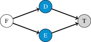
Figure 1: [d-Separation] Given the above causal DAG it holds that $F\mathchoice{\mathrel{\hbox to0.0pt{$\displaystyle\perp$\hss}\mkern 2.0mu{\displaystyle\perp}}}{\mathrel{\hbox to0.0pt{$\textstyle\perp$\hss}\mkern 2.0mu{\textstyle\perp}}}{\mathrel{\hbox to0.0pt{$\scriptstyle\perp$\hss}\mkern 2.0mu{\scriptstyle\perp}}}{\mathrel{\hbox to0.0pt{$\scriptscriptstyle\perp$\hss}\mkern 2.0mu{\scriptscriptstyle\perp}}}T\mid D,E$, or $F$ is d-separated of $T$ given $D,E$ under the faithfulness assumption. Note that $D\not\mathchoice{\mathrel{\hbox to0.0pt{$\displaystyle\perp$\hss}\mkern 2.0mu{\displaystyle\perp}}}{\mathrel{\hbox to0.0pt{$\textstyle\perp$\hss}\mkern 2.0mu{\textstyle\perp}}}{\mathrel{\hbox to0.0pt{$\scriptstyle\perp$\hss}\mkern 2.0mu{\scriptstyle\perp}}}{\mathrel{\hbox to0.0pt{$\scriptscriptstyle\perp$\hss}\mkern 2.0mu{\scriptscriptstyle\perp}}}T\mid E,F$ and $E\not\mathchoice{\mathrel{\hbox to0.0pt{$\displaystyle\perp$\hss}\mkern 2.0mu{\displaystyle\perp}}}{\mathrel{\hbox to0.0pt{$\textstyle\perp$\hss}\mkern 2.0mu{\textstyle\perp}}}{\mathrel{\hbox to0.0pt{$\scriptstyle\perp$\hss}\mkern 2.0mu{\scriptstyle\perp}}}{\mathrel{\hbox to0.0pt{$\scriptscriptstyle\perp$\hss}\mkern 2.0mu{\scriptscriptstyle\perp}}}T\mid D,F$.

For discrete data, two tests are frequently used in practice, the $G^{2}$ test (Aliferis et al.,, 2010; Schlüter,, 2014) and conditional mutual information ($\mathit{CMI}$) (Zhang et al.,, 2010). While the former is theoretically sound, it is very restrictive as it has a high sample complexity; especially when conditioning on multiple random variables. When used in algorithms to find the Markov blanket, for example, this leads to low recall, as there it is necessary to condition on larger sets of variables.

If we had access to the true distributions, conditional mutual information would be the perfect criterium for conditional independence. Estimating $\mathit{CMI}$ purely from limited observational data leads, however, to discovering spurious dependencies—in fact, it is likely to find no independence at all (Zhang et al.,, 2010). To use $\mathit{CMI}$ in practice, it is therefore necessary to set a threshold. This is not an easy task, as the threshold should depend on both the domain sizes of the involved variables as well as the sample size (Goebel et al.,, 2005). Recently, Canonne et al., (2018) showed that instead of exponentially many samples, theoretically $\mathit{CMI}$ has only a sub-linear sample complexity, although an algorithm is not provided. Closest to our approach is the work of Goebel et al., (2005) and Suzuki, (2016). The former show that the empirical mutual information follows the gamma distribution, which allows them to define a threshold based on the domain sizes of the variables and the sample size. The latter employs an asymptotic formulation to determine the the threshold for $\mathit{CMI}$.

The main problem of existing tests is that these struggle to find the right balance for limited data: either they are too restrictive and declare everything as independent or not restrictive enough and do not find any independence. To tackle this problem, we build upon algorithmic conditional independence, which has the advantage that we not only consider the statistical dependence, but also the complexity of the distribution. Although algorithmic independence is not computable, we can instantiate this ideal formulation with stochastic complexity. In essence, we compute stochastic complexity using either factorized or quotient normalized maximum likelihood (fNML and qNML) (Silander et al.,, 2008, 2018), and formulate $\mathit{SCI}$, the Stochastic complexity based Conditional Independence criterium.

Importantly, we show that we can reformulate $\mathit{SCI}$ to find a natural threshold for $\mathit{CMI}$ that works very well given limited data and diminishes given enough data. In the limit, we prove that $\mathit{SCI}$ is an asymptotically unbiased and $L_{2}$ consistent estimator of $\mathit{CMI}$. For limited data, we find that the qNML threshold behaves similar to Goebel et al., (2005)—i.e. it considers the sample size as well as the dimensionality of the data. The fNML threshold, however, additionally considers the estimated probability mass functions of the conditioning variables. In practice, this reduces the type II error. Moreover, when applying $\mathit{SCI}$ based on fNML in constraint based causal discovery algorithms, we observe a higher precision and recall than related tests. In addition, in our empirical evaluation $\mathit{SCI}$ shows a sub-linear sample complexity.

In this work we build upon and extend the basic ideas we first presented as (Marx and Vreeken,, 2018). Here we specifically focus on the theory and properties of using stochastic complexity for measuring conditional independence. Those readers that are interested in how SCI can be used in the discovery of directed Markov blankets we refer to (Marx and Vreeken,, 2018).

For conciseness, we postpone some proofs and experiments to the supplemental material. For reproducibility of our experiments we make our code available online and released an efficient version of $\mathit{SCI}$ in the R-package SCCI.

2 Conditional Independence Testing

In this section, we introduce the notation and give brief introductions to both standard statistical conditional independence testing, as well as to the notion of algorithmic conditional independence.

Given three possibly multivariate random variables $X$, $Y$ and $Z$, our goal is to test the conditional independence hypothesis $H_{0}\colon X\mathchoice{\mathrel{\hbox to0.0pt{$\displaystyle\perp$\hss}\mkern 2.0mu{\displaystyle\perp}}}{\mathrel{\hbox to0.0pt{$\textstyle\perp$\hss}\mkern 2.0mu{\textstyle\perp}}}{\mathrel{\hbox to0.0pt{$\scriptstyle\perp$\hss}\mkern 2.0mu{\scriptstyle\perp}}}{\mathrel{\hbox to0.0pt{$\scriptscriptstyle\perp$\hss}\mkern 2.0mu{\scriptscriptstyle\perp}}}Y\mid Z$ against the general alternative $H_{1}\colon X\not\mathchoice{\mathrel{\hbox to0.0pt{$\displaystyle\perp$\hss}\mkern 2.0mu{\displaystyle\perp}}}{\mathrel{\hbox to0.0pt{$\textstyle\perp$\hss}\mkern 2.0mu{\textstyle\perp}}}{\mathrel{\hbox to0.0pt{$\scriptstyle\perp$\hss}\mkern 2.0mu{\scriptstyle\perp}}}{\mathrel{\hbox to0.0pt{$\scriptscriptstyle\perp$\hss}\mkern 2.0mu{\scriptscriptstyle\perp}}}Y\mid Z$. The main goal of a good independence test is to minimize the type I and type II error. The type I error is defined as falsely rejecting the null hypothesis and the type II error is defined as falsely accepting the null hypothesis.

A well known theoretical measure for conditional independence is conditional mutual information based on Shannon entropy (Cover and Thomas,, 2006).

Definition 1.

Given random variables $X$, $Y$ and $Z$. If

$$I(X;Y\mid Z):=H(X\mid Z)-H(X\mid Z,Y)=0$$ (1)

then $X$ and $Y$ are called statistically independent given $Z$.

In theory, conditional mutual information ($\mathit{CMI}$) works perfectly as an independence test for discrete data. However, this only holds if we are given the true distributions of the random variables. In practice, those are not given. On a limited sample the plug-in estimator tends to underestimates conditional entropies, and as a consequence, the conditional mutual information is overestimated—even for completely independent data, as in the following Example.

Example 1.

Given three random variables $X_{1}$, $X_{2}$ and $Y$, with resp. domain sizes $1\,000,8$ and $4$. Suppose that we are given $1\,000$ samples over their joint distribution and find that $\hat{H}(Y\mid X_{1})=\hat{H}(Y\mid X_{2})=0$. That is, $Y$ is a deterministic function of $X_{1}$, as well as of $X_{2}$. However, as $|\mathcal{X}_{1}|=1\,000$, and given only $1\,000$ samples, it is likely that we will have only a single sample for each $v\in\mathcal{X}_{1}$. That is, finding that $\hat{H}(Y\mid X_{1})=0$ is likely due to the limited amount of samples, rather than that it depicts a true (functional) dependency, while $\hat{H}(Y\mid X_{2})=0$ is more likely to be due to a true dependency, since the number of samples $n\gg|\mathcal{X}_{2}|$—i.e. we have more evidence.

A possible solution is to set a threshold $t$ such that $X\mathchoice{\mathrel{\hbox to0.0pt{$\displaystyle\perp$\hss}\mkern 2.0mu{\displaystyle\perp}}}{\mathrel{\hbox to0.0pt{$\textstyle\perp$\hss}\mkern 2.0mu{\textstyle\perp}}}{\mathrel{\hbox to0.0pt{$\scriptstyle\perp$\hss}\mkern 2.0mu{\scriptstyle\perp}}}{\mathrel{\hbox to0.0pt{$\scriptscriptstyle\perp$\hss}\mkern 2.0mu{\scriptscriptstyle\perp}}}Y\mid Z$ if $I(X;Y\mid Z)\leq t$. Setting $t$ is, however, not an easy task, as $t$ is dependent on the quality of the entropy estimate, which by itself strongly depends on the complexity of the distribution and the given number of samples. Instead, to avoid this problem altogether, we will base our test on the notion of algorithmic independence.

2.1 Algorithmic Independence

To define algorithmic independence, we need to give a brief introduction to Kolmogorov complexity. The Kolmogorov complexity of a finite binary string $x$ is the length of the shortest binary program $p^{*}$ for a universal Turing machine $\mathcal{U}$ that generates $x$, and then halts (Kolmogorov,, 1965; Li and Vitányi,, 1993). Formally, we have

$$K(x)=\min\{|p|\mid p\in\{0,1\}^{*},\mathcal{U}(p)=x\}\;.$$

That is, program $p^{*}$ is the most succinct algorithmic description of $x$, or in other words, the ultimate lossless compressor for that string. To define algorithmic independence, we will also need conditional Kolmogorov complexity, $K(x\mid y)\leq K(x)$, which is again the length of the shortest binary program $p^{*}$ that generates $x$, and halts, but now given $y$ as input for free.

By definition, Kolmogorov complexity makes maximal use of any effective structure in $x$; structure that can be expressed more succinctly algorithmically than by printing it verbatim. As such it is the theoretical optimal measure for complexity. In this point, algorithmic independence differs from statistical independence. In contrast to purely considering the dependency between random variables, it also considers the complexity of the process behind the dependency.

Let us consider Example 1 again and let $x_{1}$, $x_{2}$, and $y$ be the binary strings representing $X_{1},X_{2}$ and $Y$. As $Y$ can be expressed as a deterministic function of $X_{1}$ or $X_{2}$, $K(y\mid x_{1})$ and $K(y\mid x_{2})$ reduce to the programs describing the corresponding function. As the domain size of $X_{2}$ is $8$ and $|\mathcal{Y}|=4$, the program to describe $Y$ from $X_{2}$ only has to describe the mapping from $8$ to $4$ values, which will be shorter than describing a mapping from $X_{1}$ to $Y$, since $|\mathcal{X}_{1}|=1\,000$—i.e. $K(y\mid x_{2})\leq K(y\mid x_{1})$ in contrast $\hat{H}(Y\mid X_{1})=\hat{H}(Y\mid X_{2})$. To reject $Y\mathchoice{\mathrel{\hbox to0.0pt{$\displaystyle\perp$\hss}\mkern 2.0mu{\displaystyle\perp}}}{\mathrel{\hbox to0.0pt{$\textstyle\perp$\hss}\mkern 2.0mu{\textstyle\perp}}}{\mathrel{\hbox to0.0pt{$\scriptstyle\perp$\hss}\mkern 2.0mu{\scriptstyle\perp}}}{\mathrel{\hbox to0.0pt{$\scriptscriptstyle\perp$\hss}\mkern 2.0mu{\scriptscriptstyle\perp}}}X\mid Z$, we test whether providing the information of $X$ leads to a shorter program than only knowing $Z$. Formally, we define algorithmic conditional independence as follows (Chaitin,, 1975).

Definition 2.

Given the strings $x,y$ and $z$, We write $z^{*}$ to denote the shortest program for $z$, and analogously $(z,y)^{*}$ for the shortest program for the concatenation of $z$ and $y$. If

$$I_{A}(x;y\mid z):=K(x\mid z^{*})-K(x\mid(z,y)^{*})\stackrel{{\scriptstyle+}}{{=}}0$$ (2)

holds up to an additive constant that is independent of the data, then $x$ and $y$ are called algorithmically independent given $z$.

Due to the halting problem Kolmogorov complexity is not computable, however, nor approximable up to arbitrary precision (Li and Vitányi,, 1993). The Minimum Description Length (MDL) principle (Grünwald,, 2007) provides a statistically well-founded approach to approximate it from above. For discrete data, this means we can use the stochastic complexity for multinomials (Kontkanen and Myllymäki,, 2007), which belongs to the class of refined MDL codes.

3 Stochastic Complexity for Multinomials

Given $n$ samples of a discrete univariate random variable $X$ with a domain $\mathcal{X}$ of $|\mathcal{X}|=k$ distinct values, $x^{n}\in\mathcal{X}^{n}$, let $\hat{\theta}(x^{n})$ denote the maximum likelihood estimator for $x^{n}$. Shtarkov, (1987) defined the mini-max optimal normalized maximum likelihood (NML)

$$P_{\mathit{NML}}(x^{n}\mid\mathcal{M}_{k})=\frac{P(x^{n}\mid\hat{\theta}(x^{n}),\mathcal{M}_{k})}{\mathcal{C}_{\mathcal{M}_{k}}^{n}}\;,$$ (3)

where the normalizing factor, or regret $\mathcal{C}_{\mathcal{M}_{k}}^{n}$, relative to the model class $\mathcal{M}_{k}$ is defined as

$$\mathcal{C}_{\mathcal{M}_{k}}^{n}=\sum_{\tilde{x}^{n}\in\mathcal{X}^{n}}P(\tilde{x}^{n}\mid\hat{\theta}(\tilde{x}^{n}),\mathcal{M}_{k})\,.$$ (4)

The sum goes over every possible $\tilde{x}^{n}$ over the domain of $X$, and for each considers the maximum likelihood for that data given model class $\mathcal{M}_{k}$. Whenever clear from context, we drop the model class to simplify the notation—i.e. we write $P_{\mathit{NML}}(x^{n})$ for $P_{\mathit{NML}}(x^{n}\mid\mathcal{M}_{k})$ and $\mathcal{C}_{k}^{n}$ to refer to $\mathcal{C}_{\mathcal{M}_{k}}^{n}$.

For discrete data, assuming a multinomial distribution, we can rewrite Eq. (3) as (Kontkanen and Myllymäki,, 2007)

$$P_{\mathit{NML}}(x^{n})=\frac{\prod_{j=1}^{k}\left(\frac{|v_{j}|}{n}\right)^{|v_{j}|}}{\mathcal{C}_{k}^{n}}\;,$$

writing $|v_{j}|$ for the frequency of value $v_{j}$ in $x^{n}$, resp. Eq. (4) as

$$\mathcal{C}_{k}^{n}=\sum_{|v_{1}|+\cdots+|v_{k}|=n}\frac{n!}{|v_{1}|!\cdots|v_{k}|!}\prod_{j=1}^{k}\left(\frac{|v_{j}|}{n}\right)^{|v_{j}|}\ .$$

Mononen and Myllymäki, (2008) derived a formula to calculate the regret in sub-linear time, meaning that the whole formula can be computed in linear time w.r.t. $n$.

We obtain the stochastic complexity for $x^{n}$ by simply taking the negative logarithm of $P_{\mathit{NML}}$, which decomposes into a Shannon-entropy and the log regret

$$\mathit{S}(x^{n}) =-\log P_{\mathit{NML}}(x^{n})\;,$$ (5)

$$=n\hat{H}(x^{n})+\log\mathcal{C}_{k}^{n}\;.$$ (6)

3.1 Conditional Stochastic Complexity

Conditional stochastic complexity can be defined in different ways. We consider factorized normalized maximum likelihood (fNML) (Silander et al.,, 2008) and quotient normalized maximum likelihood (qNML) (Silander et al.,, 2018), which are equivalent except for the regret terms.

Given $x^{n}$ and $y^{n}$ drawn from the joint distribution of two random variables $X$ and $Y$, where $k$ is the size of the domain of $X$. Conditional stochastic complexity using the fNML formulation is defined as

$$\mathit{S}_{f}(x^{n}\mid y^{n}) =\sum_{v\in\mathcal{Y}}-\log P_{\mathit{NML}}(x^{n}\mid y^{n}=v)$$ (7)

$$=\sum_{v\in\mathcal{Y}}|v|\hat{H}(x^{n}\mid y^{n}\!=\!v)+\sum_{v\in\mathcal{Y}}\log\mathcal{C}_{k}^{|v|},\;\;$$ (8)

where $y^{n}=v$ denotes the set of samples for which $Y=v$, $\mathcal{Y}$ the domain of $Y$ with domain size $l$, and $|v|$ the frequency of a value $v$ in $y^{n}$.

Analogously, we can define conditional stochastic complexity $S_{q}$ using qNML (Silander et al.,, 2018). We prove all important properties of our independence test for both fNML and qNML definitions, but for conciseness, and because $S_{f}$ performs superior in our experiments, we postpone the definition of $S_{q}$ and the related proofs to the supplemental material.

In the following, we always consider the sample size $n$ and slightly abuse the notation by replacing $\mathit{S}(x^{n})$ by $\mathit{S}(X)$, similar so for the conditional case. We refer to conditional stochastic complexity as $\mathit{S}$ and only use $\mathit{S}_{f}$ or $\mathit{S}_{q}$ whenever there is a conceptual difference. In addition, we refer to the regret terms of the conditional $\mathit{S}(X\mid Z)$ as $\mathcal{R}(X\mid Z)$, where

$$\mathcal{R}_{f}(X\mid Z)=\sum_{z\in\mathcal{Z}}\log\mathcal{C}_{|\mathcal{X}|}^{|z|}\;.$$

Next, we show that the regret term is log-concave in $n$, which is a property we need later on.

Lemma 1.

For $n\geq 1$, the regret term $\mathcal{C}_{k}^{n}$ of the multinomial stochastic complexity of a random variable with a domain size of $k\geq 2$ is log-concave in $n$.

For conciseness, we postpone the proof of Lemma 1 to the supplementary material. Based on Lemma 1 we can now introduce Theorem 1 that is essential for our proposed independence test.

Theorem 1.

Given three random variables $X$, $Y$ and $Z$, it holds that $\mathcal{R}_{f}(X\mid Z)\leq\mathcal{R}_{f}(X\mid Z,Y)$.

Proof.

Consider that $Z$ contains $p$ distinct value combinations $\{r_{1},\dots,r_{p}\}$. If we add $Y$ to $Z$, the number of distinct value combinations, $\{l_{1},\dots,\l_{q}\}$, increases to $q$, where $p\leq q$. Consequently, to show that Theorem 1 is true, it suffices to show that

$$\sum_{i=1}^{p}\log\mathcal{C}_{k}^{|r_{i}|}\leq\sum_{j=1}^{q}\log\mathcal{C}_{k}^{|l_{j}|}\,$$ (9)

where $\sum_{i=1}^{p}|r_{i}|=\sum_{j=1}^{q}|l_{j}|=n$. Next, consider w.l.o.g. that each value combination $\{r_{i}\}_{i=1,\dots,p}$ is mapped to one or more value combinations in $\{l_{1},\dots,\l_{q}\}$. Hence, Eq. (9) holds, if the $\log\mathcal{C}_{k}^{n}$ is sub-additive in $n$. Since we know from Lemma 1 that the regret term is log-concave in $n$, sub-additivity follows by definition.

Now that we have all the necessary tools, we can define our independence test in the next section.

4 Stochastic Complexity based Conditional Independence

With the above, we can now formulate our new conditional independence test, which we will refer to as the Stochastic complexity based Conditional Independence criterium, or $\mathit{SCI}$ for short.

Definition 3.

Let $X$, $Y$ and $Z$ be random variables. We say that $X\mathchoice{\mathrel{\hbox to0.0pt{$\displaystyle\perp$\hss}\mkern 2.0mu{\displaystyle\perp}}}{\mathrel{\hbox to0.0pt{$\textstyle\perp$\hss}\mkern 2.0mu{\textstyle\perp}}}{\mathrel{\hbox to0.0pt{$\scriptstyle\perp$\hss}\mkern 2.0mu{\scriptstyle\perp}}}{\mathrel{\hbox to0.0pt{$\scriptscriptstyle\perp$\hss}\mkern 2.0mu{\scriptscriptstyle\perp}}}Y\mid Z$, if

$$\mathit{SCI}(X;Y\mid Z):=\mathit{S}(X\mid Z)-\mathit{S}(X\mid Z,Y)\leq 0\;.$$ (10)

In particular, Eq. 10 can be rewritten as

$$\mathit{SCI}(X;Y\mid Z) =n\cdot I(X;Y\mid Z)$$ (11)

$$+\mathcal{R}(X\mid Z)-\mathcal{R}(X\mid Z,Y)\;.$$ (12)

From this formulation, we see that the regret terms formulate a threshold $t_{\mathit{S}}$ for conditional mutual information, where $t_{\mathit{S}}=\mathcal{R}(X\mid Z,Y)-\mathcal{R}(X\mid Z)$. From Theorem 1 we know that if we instantiate $\mathit{SCI}$ using fNML that $\mathcal{R}(X\mid Z,Y)-\mathcal{R}(X\mid Z)\geq 0$. Hence, $Y$ has to provide a significant gain such that $X\not\mathchoice{\mathrel{\hbox to0.0pt{$\displaystyle\perp$\hss}\mkern 2.0mu{\displaystyle\perp}}}{\mathrel{\hbox to0.0pt{$\textstyle\perp$\hss}\mkern 2.0mu{\textstyle\perp}}}{\mathrel{\hbox to0.0pt{$\scriptstyle\perp$\hss}\mkern 2.0mu{\scriptstyle\perp}}}{\mathrel{\hbox to0.0pt{$\scriptscriptstyle\perp$\hss}\mkern 2.0mu{\scriptscriptstyle\perp}}}Y\mid Z$—i.e. we need $\hat{H}(X\mid Z)-\hat{H}(X\mid Z,Y)>t_{\mathit{S}}/n$.

Next, we show how we can use $\mathit{SCI}$ in practice by formulating it using fNML.

4.1 Factorized SCI

To formulate our independence test based on factorized normalized maximum likelihood, we have to revisit the regret terms again. In particular, $\mathcal{R}_{f}(X\mid Z)$ is only equal to $\mathcal{R}_{f}(Y\mid Z)$, when the domain size of $X$ is equal to the domain of $Y$. Further, $\mathcal{R}_{f}(X\mid Z)-\mathcal{R}_{f}(X\mid Z,Y)$ is not guaranteed to be equal to $\mathcal{R}_{f}(Y\mid Z)-\mathcal{R}_{f}(Y\mid Z,X)$. As a consequence,

$$I_{\mathit{S}}^{f}(X;Y\mid Z):=\mathit{S}_{f}(X\mid Z)-\mathit{S}_{f}(X\mid Z,Y)$$

is not always equal to

$$I_{\mathit{S}}^{f}(Y;X\mid Z):=\mathit{S}_{f}(Y\mid Z)-\mathit{S}_{f}(Y\mid Z,X)\;.$$

To achieve symmetry, we formulate $\mathit{SCI}_{f}$ as

$$\mathit{SCI}_{f}(X;Y\mid Z):=\max\{I_{\mathit{S}}^{f}(X;Y\mid Z),I_{\mathit{S}}^{f}(Y;X\mid Z)\}$$ (13)

and say that $X\mathchoice{\mathrel{\hbox to0.0pt{$\displaystyle\perp$\hss}\mkern 2.0mu{\displaystyle\perp}}}{\mathrel{\hbox to0.0pt{$\textstyle\perp$\hss}\mkern 2.0mu{\textstyle\perp}}}{\mathrel{\hbox to0.0pt{$\scriptstyle\perp$\hss}\mkern 2.0mu{\scriptstyle\perp}}}{\mathrel{\hbox to0.0pt{$\scriptscriptstyle\perp$\hss}\mkern 2.0mu{\scriptscriptstyle\perp}}}Y\mid Z$, if $\mathit{SCI}_{f}(X;Y\mid Z)\leq 0$.

There are other ways to achieve such symmetry, such as via an alternative definition of conditional mutual information. However, as we show in detail in the supplementary, there exist serious issues with these alternatives when instantiated with fNML.

Instead of the exact fNML formulation, it is also possible to use the asymptotic approximation of stochastic complexity (Rissanen,, 1996), which was done by Suzuki, (2016) to approximate $\mathit{CMI}$. In practice, the corresponding test ($\mathit{JIC}$) is, however, very restrictive, which leads to low recall.

In the next section, we show the main properties for $\mathit{SCI}$ using fNML. Thereafter, we compare $\mathit{SCI}$ to $\mathit{CMI}$ using the threshold based on the gamma distribution (Goebel et al.,, 2005), and empirically evaluate the sample complexity of $\mathit{SCI}$.

4.2 Properties of SCI

In the following, for readability, we write $\mathit{SCI}$ to refer to properties that hold for both versions of $\mathit{SCI}$, $\mathit{SCI}_{f}$ and $\mathit{SCI}_{q}$.

First, we show that if $X\mathchoice{\mathrel{\hbox to0.0pt{$\displaystyle\perp$\hss}\mkern 2.0mu{\displaystyle\perp}}}{\mathrel{\hbox to0.0pt{$\textstyle\perp$\hss}\mkern 2.0mu{\textstyle\perp}}}{\mathrel{\hbox to0.0pt{$\scriptstyle\perp$\hss}\mkern 2.0mu{\scriptstyle\perp}}}{\mathrel{\hbox to0.0pt{$\scriptscriptstyle\perp$\hss}\mkern 2.0mu{\scriptscriptstyle\perp}}}Y\mid Z$, we have that $\mathit{SCI}(X;Y\mid Z)\leq 0$. Then, we prove that $\frac{1}{n}\mathit{SCI}$ is an asymptotically unbiased estimator of conditional mutual information and is $L_{2}$ consistent. Note that by dividing $\mathit{SCI}$ by $n$ we do not change the decisions we make as long as $n<\infty$. Since we only accept $H_{0}$ if $\mathit{SCI}\leq 0$, any positive output will still be $>0$ after dividing it by $n$.

Theorem 2.

If $X\mathchoice{\mathrel{\hbox to0.0pt{$\displaystyle\perp$\hss}\mkern 2.0mu{\displaystyle\perp}}}{\mathrel{\hbox to0.0pt{$\textstyle\perp$\hss}\mkern 2.0mu{\textstyle\perp}}}{\mathrel{\hbox to0.0pt{$\scriptstyle\perp$\hss}\mkern 2.0mu{\scriptstyle\perp}}}{\mathrel{\hbox to0.0pt{$\scriptscriptstyle\perp$\hss}\mkern 2.0mu{\scriptscriptstyle\perp}}}Y\mid Z$, $\mathit{SCI}(X;Y\mid Z)\leq 0$.

Proof.

W.l.o.g. we can assume that $I_{\mathit{S}}^{f}(X;Y\mid Z)>=I_{\mathit{S}}^{f}(Y;X\mid Z)$. Based on this, it suffices to show that $I_{\mathit{S}}^{f}(X;Y\mid Z)\leq 0$ if $X\mathchoice{\mathrel{\hbox to0.0pt{$\displaystyle\perp$\hss}\mkern 2.0mu{\displaystyle\perp}}}{\mathrel{\hbox to0.0pt{$\textstyle\perp$\hss}\mkern 2.0mu{\textstyle\perp}}}{\mathrel{\hbox to0.0pt{$\scriptstyle\perp$\hss}\mkern 2.0mu{\scriptstyle\perp}}}{\mathrel{\hbox to0.0pt{$\scriptscriptstyle\perp$\hss}\mkern 2.0mu{\scriptscriptstyle\perp}}}Y\mid Z$. As the first part of $I_{\mathit{S}}^{f}$ consists of $n\cdot I(X;Y\mid Z)$, it will be zero by definition. We know that $\mathcal{R}_{f}(X\mid Z)-\mathcal{R}_{f}(X\mid Z,Y)\leq 0$ (Theorem 1), which concludes the proof.

Next, we show that $\frac{1}{n}\mathit{SCI}$ converges against conditional mutual information and hence is an asymptotically unbiased estimator of conditional mutual information and is $L_{2}$ consistent to it.

Lemma 2.

Given three random variables $X$, $Y$ and $Z$, it holds that $\lim_{n\rightarrow\infty}\frac{1}{n}\mathit{SCI}(X;Y\mid Z)=I(X;Y\mid Z)$.

Proof.

To show the claim, we need to show that

$$\lim_{n\rightarrow\infty}I(X;Y\mid Z)+\frac{1}{n}(\mathcal{R}(X\mid Z)-\mathcal{R}(X\mid Z,Y))=0\;.$$

The proof for $I_{\mathit{S}}^{f}(Y;X\mid Z)$ follows analogously. In essence, we need to show that $\frac{1}{n}(\mathcal{R}(X\mid Z)-\mathcal{R}(X\mid Z,Y))$ goes to zero as $n$ goes to infinity. From Rissanen, (1996) we know that $\log\mathcal{C}_{k}^{n}$ asymptotically behaves like $\frac{k-1}{2}\log n+\mathcal{O}(1)$. Hence, $\frac{1}{n}\mathcal{R}(X\mid Z)$ and $\frac{1}{n}\mathcal{R}(X\mid Z,Y)$ will approach zero if $n\rightarrow\infty$.

As a corollary to Lemma 2 we find that $\frac{1}{n}\mathit{SCI}$ is an asymptotically unbiased estimator of conditional mutual information and is $L_{2}$ consistent to it.

Theorem 3.

Let $X$, $Y$ and $Z$ be discrete random variables. Then $\lim_{n\to\infty}\mathbb{E}[\frac{1}{n}\mathit{SCI}(X;Y|Z)]=I(X;Y|Z)$, i.e. $\frac{1}{n}\mathit{SCI}$ is an asymptotically unbiased estimator for conditional mutual information.

Theorem 4.

Let $X$, $Y$ and $Z$ be discrete random variables. Then $\lim_{n\to\infty}\mathbb{E}[(\frac{1}{n}\mathit{SCI}(X;Y|Z)-I(X;Y|Z))^{2}]=0$ i.e. $\frac{1}{n}\mathit{SCI}$ is an $L_{2}$ consistent estimator for conditional mutual information.

Next, we compare both of our tests to the findings of Goebel et al., (2005).

4.3 Link to Gamma Distribution

Goebel et al., (2005) estimate conditional mutual information through a second-order Taylor series and show that their estimator can be approximated with the gamma distribution. In particular, they state that

$$\hat{I}(X;Y\mid Z)\sim\Gamma\left(\frac{|\mathcal{Z}|}{2}(|\mathcal{X}|-1)(|\mathcal{Y}|-1),\frac{1}{n\ln 2}\right)\;,$$

where $\mathcal{X}$, $\mathcal{Y}$ and $\mathcal{Z}$ refer to the domains of $X$, $Y$ and $Z$. This means by selecting a significance threshold $\alpha$, we can derive a threshold for $\mathit{CMI}$ based on the gamma distribution—for convenience we call this threshold $t_{\Gamma}$. In the following, we compare $t_{\Gamma}$ against $t_{\mathit{S}}=\mathcal{R}(X\mid Z,Y)-\mathcal{R}(X\mid Z)$.

First of all, for qNML, like $t_{\Gamma}$, $t_{\mathit{S}}$ depends purely on the sample size and the domain sizes. However, we consider the difference in complexity between only conditioning $X$ on $Z$ and the complexity of conditioning $X$ on $Z$ and $Y$. For fNML, we have the additional aspect that the regret terms for both $\mathcal{R}(X\mid Z)$ and $\mathcal{R}(X\mid Z,Y)$ also relate to the probability mass functions of $Z$, and respectively the Cartesian product of $Z$ and $Y$. Recall that for $k$ being the size of the domain of $X$, we have that

$$\mathcal{R}_{f}(X\mid Z)=\sum_{z\in Z}\log\mathcal{C}_{k}^{|z|}\;.$$

As $\mathcal{C}_{k}^{n}$ is log-concave in $n$ (Lemma 1), $\mathcal{R}_{f}(X\mid Z)$ is maximal if $Z$ is uniformly distributed—i.e. it is maximal when $H(Z)$ is maximal. This is a favourable property, as the probability that $Z$ is equal to $X$ is minimal for uniform $Z$, as stated in the following Lemma (Cover and Thomas,, 2006).

Lemma 3.

If $X$ and $Y$ are i.i.d. with entropy $H(Y)$, then $P(Y=X)\geq 2^{-H(Y)}$ with equality if and only if $Y$ has a uniform distribution.

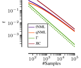
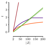
Figure 2: Threshold for $\mathit{CMI}$ using fNML, qNML, $\mathit{JIC}$ and the gamma distribution with $\alpha=0.05$ (solid) and $\alpha=0.001$ (dashed) for different sample sizes and fixed domain sizes equal to four (left) and fixed sample size of $500$ and changing domain sizes (right).

To elaborate the link between $t_{\Gamma}$ and $t_{\mathit{S}}$, we compare them empirically. In addition, we compare the results to the threshold provided from the $\mathit{JIC}$ test. First, we compare $t_{\Gamma}$ with $\alpha=0.05$ and $\alpha=0.001$ to $t_{\mathit{S}}/n$ for fNML and qNML, and $\mathit{JIC}$ on fixed domain sizes, with $|\mathcal{X}|=|\mathcal{Y}|=|\mathcal{Z}|=4$ and varying the sample sizes (see Figure 2). For fNML we computed the worst case threshold under the assumption that $Z$ is uniformly distributed. In general, the behaviour for each threshold is similar, whereas qNML, fNML and $\mathit{JIC}$ are more restrictive than $t_{\Gamma}$.

Next, we keep the sample size fix at $500$ and increase the domain sizes of $Z$ from $2$ to $200$, to simulate multiple variables in the conditioning set. Except to $\mathit{JIC}$, which seems to overpenalize in this case, we observe that fNML is most restrictive until we reach a plateau when $|\mathcal{Z}|=125$. This is due to the fact that $|\mathcal{Z}||\mathcal{Y}|=500$ and hence each data point is assigned to one value in the Cartesian product. We have that $\mathcal{R}_{f}(X\mid Z,Y)=|\mathcal{Z}||\mathcal{Y}|\mathcal{C}_{k}^{1}$.

It is important to note, however, that the thresholds that we computed for fNML assume that $Z$ and $Y$ are uniformly distributed and $Y\mathchoice{\mathrel{\hbox to0.0pt{$\displaystyle\perp$\hss}\mkern 2.0mu{\displaystyle\perp}}}{\mathrel{\hbox to0.0pt{$\textstyle\perp$\hss}\mkern 2.0mu{\textstyle\perp}}}{\mathrel{\hbox to0.0pt{$\scriptstyle\perp$\hss}\mkern 2.0mu{\scriptstyle\perp}}}{\mathrel{\hbox to0.0pt{$\scriptscriptstyle\perp$\hss}\mkern 2.0mu{\scriptscriptstyle\perp}}}Z$. In practice, when this requirement is not fulfilled, the regret term of fNML can be smaller than this value, since it is data dependent. In addition, it is possible that the number of distinct values that we observe from the joint distribution of $Z$ and $Y$ is smaller than their Cartesian product, which also reduces the difference in the regret terms for fNML.

4.4 Empirical Sample Complexity

In this section, we empirically evaluate the sample complexity of $\mathit{SCI}_{f}$, where we focus on the type I error, i.e. $H_{0}\colon X\mathchoice{\mathrel{\hbox to0.0pt{$\displaystyle\perp$\hss}\mkern 2.0mu{\displaystyle\perp}}}{\mathrel{\hbox to0.0pt{$\textstyle\perp$\hss}\mkern 2.0mu{\textstyle\perp}}}{\mathrel{\hbox to0.0pt{$\scriptstyle\perp$\hss}\mkern 2.0mu{\scriptstyle\perp}}}{\mathrel{\hbox to0.0pt{$\scriptscriptstyle\perp$\hss}\mkern 2.0mu{\scriptscriptstyle\perp}}}Y\mid Z$ is true and hence $I(X;Y\mid Z)=0$. We generate data accordingly and draw samples from the joint distribution, where we set $P(x,y,z)=\frac{1}{|\mathcal{X}||\mathcal{Y}||\mathcal{Z}|}$ for each value configuration $(x,y,z)\in\mathcal{X}\times\mathcal{Y}\times\mathcal{Z}$. Per sample size we draw $1\,000$ data sets and report the average absolute error for $\mathit{SCI}_{f}$ and the empirical estimator of CMI, $\hat{I}$. We show the results for two cases in Fig. 3. We observe that in contrast to the empirical plug-in estimator $\hat{I}$, $\mathit{SCI}_{f}$ quickly approaches zero, and that the difference is especially large for larger domain sizes.

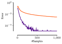
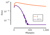
Figure 3: Error for $\mathit{SCI}_{f}$ and $\hat{I}$ compared to $I$, where $I(X;Y|Z)\mkern 1.5mu{=}\mkern 1.5mu0$. Left: $|\mathcal{X}|\mkern 1.5mu{=}\mkern 1.5mu|\mathcal{Y}|\mkern 1.5mu{=}\mkern 1.5mu2$ and $|\mathcal{Z}|\mkern 1.5mu{=}\mkern 1.5mu4$. Right: $|\mathcal{X}|\mkern 1.5mu{=}\mkern 1.5mu|\mathcal{Y}|\mkern 1.5mu{=}\mkern 1.5mu4$ and $|\mathcal{Z}|\mkern 1.5mu{=}\mkern 1.5mu16$. Values smaller than $10^{-5}$ are truncated to $10^{-5}$.

In the supplemental material we give a more in depth analysis alltogether. Our evaluation suggest that the sample complexity is sub-linear. In particular, we find that the number of samples $n$ required such that $P(|\mathit{SCI}_{f}^{n}(X;Y\mid Z)/n-I(X;Y\mid Z)|\geq\epsilon)\leq\delta$, with $\epsilon=\delta=0.05$ is smaller than $35+2|\mathcal{X}||\mathcal{Y}|^{2/3}(|\mathcal{Z}|+1)$.

To illustrate this, consider the left example in Figure 3 again. We observe that for $\epsilon=\delta=0.05$, $n$ needs to be at least $52$, which is smaller than the value from our empirical bound function, that is equal to $67$. If we require $\epsilon=0.01$ and $\delta=0.05$, we observe that $n$ must be at least $72$. In comparison, for $\hat{I}$, $n$ needs to be at least $140$ for $\epsilon=0.05$ and $684$ for $\epsilon=0.01$.

4.5 Discussion

The main idea for our independence test is to approximate conditional mutual information through algorithmic conditional independence. In particular, we estimate conditional entropy with stochastic complexity. We recommend $\mathit{SCI}_{f}$, since the regret for the entropy term does not only depend on the sample size and the domain sizes of the corresponding random variables, but also on the probability mass function of the conditioning variables. In particular, when fixing the domain sizes and the sample size, higher thresholds are assigned to conditioning variables that are unlikely to be equal to the target variable.

By assuming a uniform distribution for the conditioning variables and hence eliminating this data dependence from $\mathit{SCI}_{f}$, it behaves similar to $\mathit{SCI}_{q}$ and $\mathit{CMI}$ where the threshold is derived from the gamma distribution (Goebel et al.,, 2005). $\mathit{SCI}_{f}$ is more restrictive and the penalty terms of all three decrease exponentially w.r.t. the sample size.

$\mathit{SCI}$ can also be extended for sparsification, as is possible to derive an analytical p-value for the significance of a decision using the no-hypercompression inequality (Grünwald,, 2007; Marx and Vreeken,, 2017).

Last, note that as we here instantiate $\mathit{SCI}$ using stochastic complexity for multinomials, we implicitly assume that the data follows a multinomial distribution. In this light, it is important to note that stochastic complexity is a mini-max optimal refined MDL code (Grünwald,, 2007). This means that for any data, we obtain a score that is within a constant term from the best score attainable given our model class. The experiments verify that indeed, $\mathit{SCI}$ performs very well, even when the data is sampled adversarially.

5 Experiments

In this section, we empirically evaluate $\mathit{SCI}$ based on fNML and compare it to the alternative formulation using qNML. In addition, we compare it to the $G^{2}$ test from the pcalg R package (Kalisch et al.,, 2012), $\mathit{CMI}_{\Gamma}$ (Goebel et al.,, 2005) and $\mathit{JIC}$ (Suzuki,, 2016).

5.1 Identifying d-Separation

To test whether $\mathit{SCI}$ can reliably distinguish between independence and dependence, we generate data as depicted in Figure 1, where we draw $F$ from a uniform distribution and model a dependency from $X$ to $Y$ by simply assigning uniformly at random each $x\in\mathcal{X}$ to a $y\in\mathcal{Y}$. We set the domain size for each variable to $4$ and generate data under various samples sizes ($100$–$2\,500$) and additive uniform noise settings ($0\%$–$95\%$). For each setup we generate $200$ data sets and assess the accuracy. In particular, we report the correct identifications of $F\mathchoice{\mathrel{\hbox to0.0pt{$\displaystyle\perp$\hss}\mkern 2.0mu{\displaystyle\perp}}}{\mathrel{\hbox to0.0pt{$\textstyle\perp$\hss}\mkern 2.0mu{\textstyle\perp}}}{\mathrel{\hbox to0.0pt{$\scriptstyle\perp$\hss}\mkern 2.0mu{\scriptstyle\perp}}}{\mathrel{\hbox to0.0pt{$\scriptscriptstyle\perp$\hss}\mkern 2.0mu{\scriptscriptstyle\perp}}}T\mid D,E$ as the true positive rate and the false identifications $D\mathchoice{\mathrel{\hbox to0.0pt{$\displaystyle\perp$\hss}\mkern 2.0mu{\displaystyle\perp}}}{\mathrel{\hbox to0.0pt{$\textstyle\perp$\hss}\mkern 2.0mu{\textstyle\perp}}}{\mathrel{\hbox to0.0pt{$\scriptstyle\perp$\hss}\mkern 2.0mu{\scriptstyle\perp}}}{\mathrel{\hbox to0.0pt{$\scriptscriptstyle\perp$\hss}\mkern 2.0mu{\scriptscriptstyle\perp}}}T\mid E,F$ or $E\mathchoice{\mathrel{\hbox to0.0pt{$\displaystyle\perp$\hss}\mkern 2.0mu{\displaystyle\perp}}}{\mathrel{\hbox to0.0pt{$\textstyle\perp$\hss}\mkern 2.0mu{\textstyle\perp}}}{\mathrel{\hbox to0.0pt{$\scriptstyle\perp$\hss}\mkern 2.0mu{\scriptstyle\perp}}}{\mathrel{\hbox to0.0pt{$\scriptscriptstyle\perp$\hss}\mkern 2.0mu{\scriptscriptstyle\perp}}}T\mid D,F$ as false positive rate.​ For the $G^{2}$ test and $\mathit{CMI}_{\Gamma}$ we select $\alpha=0.05$, however, we found no significant differences for $\alpha=0.01$.

In the interest of space we only plot the accuracy of the best performing competitors in Figure 4 and report the remaining results as well as the true and false positive rates for each approach in the supplemental material. Overall, we observe that $\mathit{SCI}_{f}$ performs near perfect for less than $70\%$ additive noise. When adding $70\%$ or more noise, the type II error increases. Those results are even better than expected as from our empirical bound function we would suggest that at least $378$ samples are required to have reliable results for this data set. $\mathit{SCI}_{q}$ has a similar but slightly worse performance. In contrast, $\mathit{CMI}_{\Gamma}$ only performs well for less than $30\%$ noise and fails to identify true independencies after more than $30\%$ noise has been added, which leads to a high type I error. The $G^{2}$ test has problems with sample sizes up to $500$ and performs inconsistently given more than $35\%$ noise. Note that we forced $G^{2}$ to decide for every sample size, while the minimum number of samples recommended for $G^{2}$ on this data set would be $1\,440$, which corresponds to $10(|\mathcal{X}|-1)(|\mathcal{Y}|-1)(|\mathcal{Z}|)$.

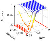
(a) $\mathit{SCI}_{f}$

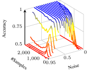
(b) $\mathit{SCI}_{q}$

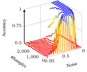
(c) $\mathit{CMI}_{\Gamma}$

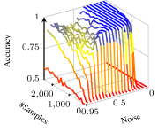
(d) $G^{2}$

Figure 4: [Higher is better] Accuracy of $\mathit{SCI}_{f}$, $\mathit{SCI}_{q}$, $\mathit{CMI}_{\Gamma}$ and $G^{2}$ for identifying $d$-separation using varying samples sizes and additive noise percentages, where a noise level of $0.95$ refers to $95\%$ additive noise.

5.2 Changing the Domain Size

Using the same data generator as above, we now consider a different setup. We fix the sample size to $2\;000$ and use only $10\%$ additive noise—a setup where all tests performed well. What we change is the domain size of the source $F$ from $2$ to $20$ while also restricting the domain sizes of the remaining variable to the same size. For each setup we generate $200$ data sets.

From the results in Figure 5 we can clearly see that only $\mathit{SCI}_{f}$ is able to deal with larger domain sizes as for all other test, the false positive rate is at $100\%$ for larger domain sizes, resulting in an accuracy of $50\%$.

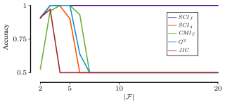
Figure 5: [Higher is better] d-Separation with $2\,000$ samples and $10\%$ noise on different domain sizes of the source node $F$.

5.3 Plug and Play with SCI

Last, we want to show how $\mathit{SCI}$ performs in practice. To do this, we run the stable PC algorithm (Kalisch et al.,, 2012; Colombo and Maathuis,, 2014) on the Alarm network (Scutari and Denis,, 2014) from which we generate data with different sample sizes and average over the results of $10$ runs for each sample size. We equip the stable PC algorithm with $\mathit{SCI}_{f}$, $\mathit{SCI}_{q}$, $\mathit{JIC}$, $\mathit{CMI}_{\Gamma}$ and the default, the $G^{2}$ test, and plot the average $F1$ score over the undirected graphs in Figure 6. We observe that our proposed test, $\mathit{SCI}_{f}$ outperforms the other tests for each sample size with a large margin and especially for small sample sizes.

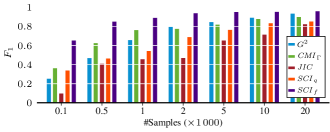
Figure 6: [Higher is better] $F_{1}$ score on undirected edges for stable PC using $\mathit{SCI}_{f}$, $\mathit{SCI}_{q}$, $\mathit{JIC}$, $\mathit{CMI}_{\Gamma}$ and $G^{2}$ on the Alarm network for different sample sizes

As a second practical test, we compute the Markov blanket for each node in the Alarm network and report the precision and recall. To find the Markov blankets, we run the PCMB algorithm (Peña et al.,, 2007) with the four independence tests. We plot the precision and recall for each variant in Figure 7. We observe that again $\mathit{SCI}_{f}$ performs best—especially with regard to recall. As for Markov blankets of size $k$ it is necessary to condition on at least $k-1$ variables, this advantage in recall can be linked back to $\mathit{SCI}_{f}$ being able to correctly detect dependencies for larger domain sizes.

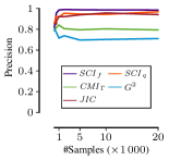
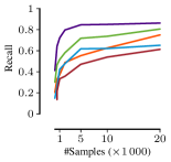
Figure 7: [Higher is better] Precision (left) and recall (right) for PCMB using $\mathit{SCI}_{f}$, $\mathit{SCI}_{q}$, $\mathit{JIC}$, $\mathit{CMI}_{\Gamma}$ and $G^{2}$ to identify all Markov blankets in the Alarm network for different sample sizes.

6 Conclusion

In this paper we introduced $\mathit{SCI}$, a new conditional independence test for discrete data. We derive $\mathit{SCI}$ from algorithmic conditional independence and show that it is an unbiased asymptotic estimator for conditional mutual information ($\mathit{CMI}$). Further, we show how to use $\mathit{SCI}$ to find a threshold for $\mathit{CMI}$ and compare it to thresholds drawn from the gamma distribution.

In particular, we propose to instantiate $\mathit{SCI}$ using fNML as in contrast to using qNML or thresholds drawn from the gamma distribution, fNML does not only make use of the sample size and domain sizes of the involved variables, but also utilizes the empirical probability mass function of the conditioning variable. Moreover, we observe that $\mathit{SCI}_{f}$ clearly outperforms its competitors on both synthetic and real world data. Last but not least, our empirical evaluations suggest that $\mathit{SCI}$ has a sub-linear sample complexity, which we would like to theoretically validate in future work.

Acknowledgements

The authors would like to thank David Kaltenpoth for insightful discussions. Alexander Marx is supported by the International Max Planck Research School for Computer Science (IMPRS-CS). Both authors are supported by the Cluster of Excellence on “Multimodal Computing and Interaction” within the Excellence Initiative of the German Federal Government.

Appendix A Extended Theory

A.1 Proof of Lemma 1

Proof.

To improve the readability of this proof, we write $\mathcal{C}_{L}^{n}$ as shorthand for $\mathcal{C}_{\mathcal{M}_{L}}^{n}$ of a random variable with a domain size of $L$.

Since $n$ is an integer, each $\mathcal{C}_{L}^{n}>0$ and $\mathcal{C}_{L}^{0}=1$, we can prove Lemma 1, by showing that the fraction $\mathcal{C}_{L}^{n}/\mathcal{C}_{L}^{n-1}$ is decreasing for $n\geq 1$, when $n$ increases.

We know from Mononen and Myllymäki, (2008) that $\mathcal{C}_{L}^{n}$ can be written as the sum

$$\mathcal{C}_{L}^{n}=\sum_{k=0}^{n}m(k,n)=\sum_{k=0}^{n}\frac{n^{\mspace{2.0mu}\underline{\mspace{-2.0mu}k\mspace{-2.0mu}}\mspace{2.0mu}}(L-1)^{\mspace{2.0mu}\overline{\mspace{-2.0mu}k\mspace{-2.0mu}}\mspace{2.0mu}}}{n^{k}k!}\;,$$ (14)

where $x^{\mspace{2.0mu}\underline{\mspace{-2.0mu}k\mspace{-2.0mu}}\mspace{2.0mu}}$ represent falling factorials and $x^{\mspace{2.0mu}\overline{\mspace{-2.0mu}k\mspace{-2.0mu}}\mspace{2.0mu}}$ rising factorials. Further, they show that for fixed $n$ we can write $m(k,n)$ as

$$m(k,n)=m(k-1,n)\frac{(n-k+1)(k+L-2)}{nk}\;,$$ (15)

where $m(0,n)$ is equal to $1$. It is easy to see that from $n=1$ to $n=2$ the fraction $\mathcal{C}_{L}^{n}/\mathcal{C}_{L}^{n-1}$ decreases, as $\mathcal{C}_{L}^{0}=1$, $\mathcal{C}_{L}^{1}=L$ and $\mathcal{C}_{L}^{2}=L+L(L-1)/2$. In the following, we will show the general case. We rewrite the fraction as follows.

$$\frac{\mathcal{C}_{L}^{n}}{\mathcal{C}_{L}^{n-1}} =\frac{\sum_{k=0}^{n}m(k,n)}{\sum_{k=0}^{n-1}m(k,n-1)}$$ (16)

$$=\frac{\sum_{k=0}^{n-1}m(k,n)}{\sum_{k=0}^{n-1}m(k,n-1)}+\frac{m(n,n)}{\sum_{k=0}^{n-1}m(k,n-1)}$$ (17)

Next, we will show that both parts of the sum in Eq. 17 are decreasing when $n$ increases. We start with the left part, which we rewrite to

$$\frac{\sum_{k=0}^{n-1}m(k,n)}{\sum_{k=0}^{n-1}m(k,n-1)} =\frac{\sum_{k=0}^{n-1}m(k,n-1)+\sum_{k=0}^{n-1}\left(m(k,n)-m(k,n-1)\right)}{\sum_{k=0}^{n-1}m(k,n-1)}$$ (18)

$$=1+\frac{\sum_{k=0}^{n-1}\frac{(L-1)^{\mspace{2.0mu}\overline{\mspace{-2.0mu}k\mspace{-2.0mu}}\mspace{2.0mu}}}{k!}\left(\frac{n^{\mspace{2.0mu}\underline{\mspace{-2.0mu}k\mspace{-2.0mu}}\mspace{2.0mu}}}{n^{k}}-\frac{(n-1)^{\mspace{2.0mu}\underline{\mspace{-2.0mu}k\mspace{-2.0mu}}\mspace{2.0mu}}}{(n-1)^{k}}\right)}{\sum_{k=0}^{n-1}m(k,n-1)}\;.$$ (19)

When $n$ increases, each term of the sum in the numerator in Eq. 19 decreases, while each element of the sum in the denominator increases. Hence, the whole term is decreasing. In the next step, we show that the right term in Eq. 17 also decreases when $n$ increases. It holds that

$$\frac{m(n,n)}{\sum_{k=0}^{n-1}m(k,n-1)}\geq\frac{m(n,n)}{m(n-1,n-1)}\;.$$

Using Eq. 15 we can reformulate the term as follows.

$$\frac{\frac{n+L-2}{n^{2}}m(n-1,n)}{m(n-1,n-1)}=\frac{n+L-2}{n^{2}}\left(1+\frac{m(n-1,n)-m(n-1,n-1)}{m(n-1,n-1)}\right)$$ (20)

After rewriting, we have that $\frac{n+L-2}{n^{2}}$ is definitely decreasing with increasing $n$. For the right part of the product, we can argue the same way as for Eq. 19. Hence the whole term is decreasing, which concludes the proof.

A.2 Quotient SCI

Conditional stochastic complexity can also be defined via quotient normalized maximum likelihood (qNML), which is defined as follows

$$\mathit{S}_{q}(x^{n}\mid y^{n})=\sum_{v\in\mathcal{Y}}|v|\hat{H}(x^{n}\mid y^{n}\!=\!v)+\log\frac{\mathcal{C}_{|\mathcal{X}|\cdot|\mathcal{Y}|}^{n}}{\mathcal{C}_{|\mathcal{Y}|}^{n}}\;.$$ (21)

We refer to the regret term of $\mathit{S}_{q}(X\mid Z)$ with

$$\mathcal{R}_{q}(X\mid Z)=\log\frac{\mathcal{C}_{|\mathcal{X}|\cdot|\mathcal{Z}|}^{n}}{\mathcal{C}_{|\mathcal{Z}|}^{n}}\;.$$

Analogously to Theorem 1 for fNML, we can define the following theorem for qNML.

Theorem 5.

Given three random variables $X$, $Y$ and $Z$, it holds that $\mathcal{R}_{q}(X\mid Z)\leq\mathcal{R}_{q}(X\mid Z,Y)$.

Proof.

Consider $n$ samples of three random variables $X$, $Y$ and $Z$, with corresponding domain sizes $k$, $p$ and $q$. It should hold that

$$\mathcal{R}_{q}(X\mid Z) \leq\mathcal{R}_{q}(X\mid Z,Y)$$ (22)

$$\Leftrightarrow\log\frac{\mathcal{C}_{kq}^{n}}{\mathcal{C}_{q}^{n}} \leq\log\frac{\mathcal{C}_{kpq}^{n}}{\mathcal{C}_{pq}^{n}}\;.$$ (23)

We know from Silander et al., (2018) that for $p\in\mathbb{N},p\geq 2$, the function $q\mapsto\frac{\mathcal{C}_{p\cdot q}^{n}}{\mathcal{C}_{q}^{n}}$ is increasing for every $q\geq 2$. This suffices to proof the statement above.

To formulate $\mathit{SCI}$ using quotient normalized maximum likelihood, we can straightforwardly replace $\mathit{S}$ with $\mathit{S}_{q}$ in the independence criterium—i.e.

$$\mathit{SCI}_{q}(X;Y\mid Z):=\mathit{S}_{q}(X\mid Z)-\mathit{S}_{q}(X\mid Z,Y)$$ (24)

and say that $X\mathchoice{\mathrel{\hbox to0.0pt{$\displaystyle\perp$\hss}\mkern 2.0mu{\displaystyle\perp}}}{\mathrel{\hbox to0.0pt{$\textstyle\perp$\hss}\mkern 2.0mu{\textstyle\perp}}}{\mathrel{\hbox to0.0pt{$\scriptstyle\perp$\hss}\mkern 2.0mu{\scriptstyle\perp}}}{\mathrel{\hbox to0.0pt{$\scriptscriptstyle\perp$\hss}\mkern 2.0mu{\scriptscriptstyle\perp}}}Y\mid Z$, if $\mathit{SCI}_{q}(X;Y\mid Z)\leq 0$. By writing down the regret terms for $\mathit{SCI}_{q}(X;Y\mid Z)$ and $\mathit{SCI}_{q}(Y;X\mid Z)$, we can see that they are equal and hence $\mathit{SCI}_{q}$ is symmetric, that is, $\mathit{SCI}_{q}(X;Y\mid Z)=\mathit{SCI}_{q}(Y;X\mid Z)$.

Since we showed that Theorem 5 holds for qNML, Theorems 2-4 can also be proven for qNML using the same arguments as for fNML.

A.3 Alternative Symmetry Correction for Factorized SCI

To instantiate $\mathit{SCI}$ using fNML, we take the maximum between $I_{\mathit{S}}^{f}(X;Y\mid Z)$ and $I_{\mathit{S}}^{f}(Y;X\mid Z)$ to achieve symmetry. We could also achieve symmetry when we base our formulation on an alternative formulation of conditional mutual information, that is

$$\mathit{CMI}(X;Y\mid Z)=H(X\mid Z)+H(Y\mid Z)-H(X,Y\mid Z)\;.$$ (25)

In particular, we formulate our alternative test by replacing the conditional entropies in Eq. 25 with stochastic complexity based on fNML

$$\mathit{SCI}_{\textit{fs}}(X;Y\mid Z)=\mathit{S}_{f}(X\mid Z)+\mathit{S}_{f}(Y\mid Z)-\mathit{S}_{f}(X,Y\mid Z)\;.$$ (26)

By writing down the regret terms, we see that $\mathit{SCI}_{\textit{fs}}(X;Y\mid Z)=\mathit{SCI}_{\textit{fs}}(Y;X\mid Z)$. In particular, if we only consider the regret terms, we get

$$\sum_{z\in Z}\left(\mathcal{C}_{|\mathcal{X}|}^{|z|}+\mathcal{C}_{|\mathcal{Y}|}^{|z|}-\mathcal{C}_{|\mathcal{X}||\mathcal{Y}|}^{|z|}\right)\;.$$ (27)

From Eq. 27 we see that all regret terms depend on the factorization given $Z$. For $I_{\mathit{S}}^{f}(X;Y\mid Z)$, however, we compare the factorizations of $X$ given only $Z$ to the one given $Z$ and $Y$, and similarly so for $I_{\mathit{S}}^{f}(Y;X\mid Z)$. In addition, for $\mathit{SCI}_{f}$ all regret terms correspond to the same domain, either to the domain of $X$ or $Y$, whereas for $\mathit{SCI}_{\textit{fs}}$ the regret terms are based on $X$, $Y$ and the Cartesian product of them. Since the last regret term of $\mathit{SCI}_{\textit{fs}}$ is based on the Cartesian product of $X$ and $Y$ it performs worse than $\mathit{SCI}_{f}$ for large domain sizes. This can also be seen in Figure 8, for which we conducted the same experiment as in Section 5.2, but also applied $\mathit{SCI}_{\textit{fs}}$. $\mathit{SCI}_{q}$ exhibits similar behaviour like $\mathit{SCI}_{\textit{fs}}$, as it also considers products of domain sizes.

There also exists a third way to formulate $\mathit{CMI}$, i.e.

$$\mathit{CMI}(X;Y\mid Z)=H(X,Z)+H(Y,Z)-H(X,Y,Z)-H(Z)\;.$$ (28)

When we replace all entropy terms with the stochastic complexity in Eq. 28, we would get an equivalent formulation to $\mathit{SCI}_{q}$, as the regret terms would sum up to exactly the same values. Hence, we do not elaborate further on this alternative.

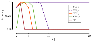
Figure 8: [Higher is better] d-Separation with $2\,000$ samples and $10\%$ noise on different domain sizes of the source node $F$.

Appendix B Experiments

In this section, we provide more details to the true positive and false positive rates w.r.t. d-separation. Further, we show how well $\mathit{SCI}$ and its competitors can recover multiple parents with and without additional noise variables in the conditioning set.

B.1 TPR and FPR for d-Separation

In Section 5.1 we analyzed the accuracy of $\mathit{SCI}_{f}$, $\mathit{SCI}_{q}$, $\mathit{CMI}_{\Gamma}$ and $G^{2}$ for identifying d-separation. In Figure 9, we plot the true and false positive rates to the corresponding experiment. In addition, we also provide the results for $\mathit{SCI}_{\textit{fs}}$ and $\mathit{CMI}_{\Gamma}$ with $\alpha=0.001$. Since we did not provide the accuracy of $\mathit{JIC}$ for this experiment in the main body of the paper, we plot the accuracy, true and false positive rates of $\mathit{JIC}$ in Figure 11 and analyze those results at the end of this section.

From Figure 9, we see that $\mathit{SCI}_{f}$ and $\mathit{SCI}_{\textit{fs}}$ perform best. Only for very high noise setups ($\geq 70\%$) they start to flag everything as independent. The $G^{2}$ test struggles with small sample sizes. It needs more than $500$ and is inconsistent given more than $35\%$ noise. Note that we forced $G^{2}$ to decide for every sample size, while the minimum number of samples recommended for $G^{2}$ on this data set would be $1\,440$, which corresponds to $10(|\mathcal{X}|-1)(|\mathcal{Y}|-1)|\mathcal{Z}|$ (Kalisch et al.,, 2012). Further, we observe that there is barely any difference between $\mathit{CMI}_{\Gamma}$ using $\alpha=0.05$ or $\alpha=0.001$ as a significance level. After more than $20\%$ noise has been added, $\mathit{CMI}_{\Gamma}$ starts to flag everything as dependent.

Next, we also show the accuracy for identifying d-separation for $\mathit{CMI}$ with zero as threshold in Figure 10. Overall, it performs very poorly, which raises from the fact that it barely finds any independence. In addition to the accuracy of $\mathit{CMI}$, we also plot the average value that $\mathit{CMI}$ reports for the true positive case ($F\mathchoice{\mathrel{\hbox to0.0pt{$\displaystyle\perp$\hss}\mkern 2.0mu{\displaystyle\perp}}}{\mathrel{\hbox to0.0pt{$\textstyle\perp$\hss}\mkern 2.0mu{\textstyle\perp}}}{\mathrel{\hbox to0.0pt{$\scriptstyle\perp$\hss}\mkern 2.0mu{\scriptstyle\perp}}}{\mathrel{\hbox to0.0pt{$\scriptscriptstyle\perp$\hss}\mkern 2.0mu{\scriptscriptstyle\perp}}}T\mid D,E$), where it should be equal to zero. It can be seen that it is dependent on the noise level as well as the sample size. This could explain, why $\mathit{SCI}_{f}$ performs best on the d-separation data. Since the noise is uniform, the threshold for $\mathit{SCI}_{f}$ is likely to be higher the more noise has been added.

The $\mathit{JIC}$ test has the opposite problem. For the d-separation scenario that we picked it is too restrictive and falsely detects independencies where the ground truth is dependent, as shown in Figure 11. As the discrete version of $\mathit{JIC}$ is calculated from the empirical entropies and a penalizing term based on the asymptotic formulation of stochastic complexity—i.e.

$$\mathit{JIC}(X;Y\mid Z):=\max\{\hat{I}(X;Y\mid Z)-\frac{(|\mathcal{X}|-1)(|\mathcal{Y}|-1)|\mathcal{Z}|}{2n}\log n,0\}\,,$$

it penalizes quite strongly in our example since $|\mathcal{Z}|=16$. As $\mathit{JIC}$ is based on an asymptotic formulation of stochastic complexity, we expect it to perform better given more data.

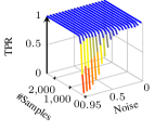
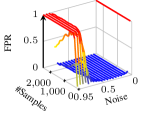
(a) $\mathit{SCI}_{f}$

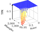
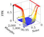
(b) $\mathit{SCI}_{q}$

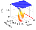
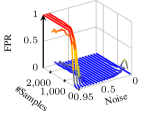
(c) $\mathit{SCI}_{\textit{fs}}$

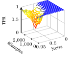
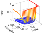
(d) $G^{2}$

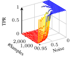
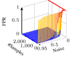
(e) $\Gamma_{.05}$

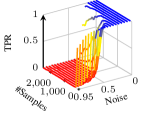
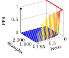
(f) $\Gamma_{.001}$

Figure 9: True positive (TPR) and false positive rates (FPR) of $\mathit{SCI}_{f}$, $\mathit{SCI}_{q}$, $\mathit{SCI}_{\textit{fs}}$, $G^{2}$ and $\mathit{CMI}_{\Gamma}$ with $\alpha=0.05$ ($\Gamma_{.05}$) and $\alpha=0.001$ ($\Gamma_{.001}$) for identifying d-separation. We use varying samples sizes and additive noise percentages, where a noise level of $0.95$ refers to $95\%$ additive noise.

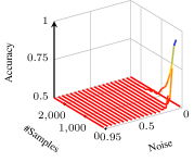
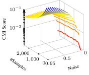
Figure 10: Accuracy of $\mathit{CMI}$ (left) and the average value returned by $\mathit{CMI}$ for the true independent case (right) for varying samples sizes and additive noise percentages. $I(F;T\mid D,E)$ is larger for small sample sizes.

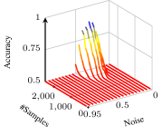
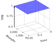
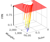
Figure 11: Accuracy, true positive (TPR) and false positive rates (FPR) of $\mathit{JIC}$ for identifying d-separation. We use varying samples sizes and additive noise percentages, where a noise level of $0.95$ refers to $95\%$ additive noise.

B.2 Identifying the Parents

In this experiment, we test the type II error. This we do by generating a certain number of parents $\mathit{PA}_{T}$ from which we generate a target node $T$. To generate the parents, we use either a

• uniform distribution with a domain size $d$ drawn uniformly with $d\sim\text{unif}(2,5)$,

• geometric distribution with parameter $p\sim\text{unif}(0.6,0.8)$,

• hyper-geometric distribution with parameter $K\sim\text{unif}(4,6)$, or

• poisson distribution with parameter $\lambda\sim\text{unif}(1,2)$.

Given the parents, we generate $T$ as a mapping from the Cartesian product of the parents to $T$ plus $10\%$ additive uniform noise. Then we generate for each distribution $200$ data sets with $2\;000$ samples, per number of parents $k\in\{2,\dots,7\}$. We apply $\mathit{SCI}_{f}$, $\mathit{SCI}_{q}$, $\mathit{CMI}_{\Gamma}$ and $G^{2}$ on each data set and we check for each $p\in\mathit{PA}_{T}$ whether they output the correct result, that is, $p\not\mathchoice{\mathrel{\hbox to0.0pt{$\displaystyle\perp$\hss}\mkern 2.0mu{\displaystyle\perp}}}{\mathrel{\hbox to0.0pt{$\textstyle\perp$\hss}\mkern 2.0mu{\textstyle\perp}}}{\mathrel{\hbox to0.0pt{$\scriptstyle\perp$\hss}\mkern 2.0mu{\scriptstyle\perp}}}{\mathrel{\hbox to0.0pt{$\scriptscriptstyle\perp$\hss}\mkern 2.0mu{\scriptscriptstyle\perp}}}T\mid\mathit{PA}_{T}\backslash\{p\}$.

We plot the averaged results for each $k$ in Figure 12. It can clearly be observed that $\mathit{SCI}_{f}$ performs best and still has near to $100\%$ accuracy for seven parents. Although not plotted here, we can add that the competitors struggled most with the data drawn from the poisson distribution. We assume that this is due to the fact that the domain sizes for these data sets were on average larger than for all other tested distributions.

In the next experiment, we generate parents and target in the same way as mentioned above, whereas we now fix the number of parents to three. In addition, we generate $k\in\{1,\dots,7\}$ random variables $N$ that are drawn jointly independent from $T$ and $\mathit{PA}_{T}$ and are uniformly distributed as described above. Then we test whether the conditional independence tests under consideration can still identify for each $p\in\mathit{PA}_{T}$ that $p\not\mathchoice{\mathrel{\hbox to0.0pt{$\displaystyle\perp$\hss}\mkern 2.0mu{\displaystyle\perp}}}{\mathrel{\hbox to0.0pt{$\textstyle\perp$\hss}\mkern 2.0mu{\textstyle\perp}}}{\mathrel{\hbox to0.0pt{$\scriptstyle\perp$\hss}\mkern 2.0mu{\scriptstyle\perp}}}{\mathrel{\hbox to0.0pt{$\scriptscriptstyle\perp$\hss}\mkern 2.0mu{\scriptscriptstyle\perp}}}T\mid N\cup\mathit{PA}_{T}\backslash\{p\}$.

The averaged results for $G^{2}$, $\mathit{JIC}$, $\mathit{SCI}_{f}$, $\mathit{SCI}_{q}$ and $\mathit{CMI}_{\Gamma}$ are plotted in Figure 12. Notice that the results for $G^{2}$ are barely visible, as they are close to zero for each setup. In general, the trend that we observe is similar to the previous experiment, except that the differences between $\mathit{SCI}_{f}$ and its competitors are even larger.

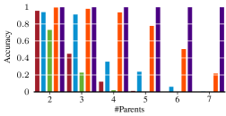
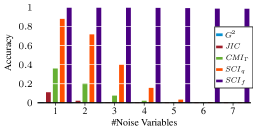
Figure 12: Left: Percentage of parents identified, where we start with only two parents and increase the number of parents to seven. Right: Percentage of parents identified, where we always use three parents, add independently drawn noise variables to the conditioning set.

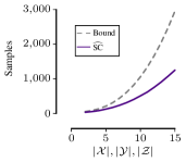
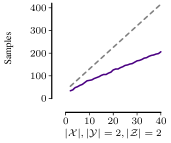
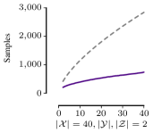
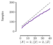
Figure 13: Estimated sample complexities for independently generated data s.t. $P(|\mathit{SCI}_{f}^{n}/n-I|\geq 0.05)\leq 0.05$ and the suggested bound function that is calculated as $35+2|\mathcal{X}||\mathcal{Y}|^{\frac{2}{3}}(|\mathcal{Z}|+1)$. For all setups, increasing the domain size of $X$, $Y$, $Z$ together or independently, the bound function is larger than the empirical value.

B.3 Empirical Sample Complexity

To give an intuition to the sample complexity of $\mathit{SCI}$, we provide an empirical evaluation. The goal of this section is to show that there exists a bound for the sample complexity of $\mathit{SCI}$, that is sub-linear w.r.t the size Cartesian product of the domain sizes and always larger than the bounds calculated from synthetic data. However, we do not argue that this is the minimal bound that can be found, nor that it is impossible to pass the bound, as we can only evaluate a subset of all possible data sets. What makes us optimistic is that it has been shown that there exists an algorithm with sub-linear sample complexity to estimate $\mathit{CMI}$ (Canonne et al.,, 2018).

The problem that we would like to solve is to provide a formula that calculates the number of samples $n$ such that $P(|\mathit{SCI}_{f}^{n}(X;Y\mid Z)-I(X;Y\mid Z)|\geq\epsilon)\leq\delta$, for small $\epsilon$ and $\delta$. Thereby, we focus on an $n$ such that the probability of making a type I error, i.e. rejecting independence when $H_{0}\colon X\mathchoice{\mathrel{\hbox to0.0pt{$\displaystyle\perp$\hss}\mkern 2.0mu{\displaystyle\perp}}}{\mathrel{\hbox to0.0pt{$\textstyle\perp$\hss}\mkern 2.0mu{\textstyle\perp}}}{\mathrel{\hbox to0.0pt{$\scriptstyle\perp$\hss}\mkern 2.0mu{\scriptstyle\perp}}}{\mathrel{\hbox to0.0pt{$\scriptscriptstyle\perp$\hss}\mkern 2.0mu{\scriptscriptstyle\perp}}}Y\mid Z$ is true, is low. In our empirical evaluation, we set $\epsilon=\delta=0.05$ and draw samples from data with the ground truth $I(X;Y\mid Z)=0$ by assigning equal probabilities to each value combination of $X$, $Y$ and $Z$—i.e. we set $P(x,y,z)=\frac{1}{|\mathcal{X}||\mathcal{Y}||\mathcal{Z}|}$ for each value configuration $(x,y,z)\in\mathcal{X}\times\mathcal{Y}\times\mathcal{Z}$. We conduct empirical evaluations for varying domain sizes of $X$, $Y$ and $Z$, where we define w.l.o.g. $|\mathcal{X}|\geq|\mathcal{Y}|$, as the test is symmetric. For each combination of domain sizes, we calculate $P(|\mathit{SCI}_{f}^{n}(X;Y\mid Z)-I(X;Y\mid Z)|\geq\epsilon)=P(\mathit{SCI}_{f}^{n}(X;Y\mid Z)\geq 0.05)\leq 0.05$ as follows: We start with a small $n$, e.g. $2$, generate $1\;000$ data sets and check if over those data sets $P(\mathit{SCI}_{f}^{n}(X;Y\mid Z)\geq 0.05)\leq 0.05$ holds. If not, we increase $n$ by the minimum domain size of $X$, $Y$ and $Z$. We repeat this procedure until we reach an $n$, for which $P(\mathit{SCI}_{f}^{n}(X;Y\mid Z)\geq 0.05)\leq 0.05$ holds and report this $n$.

In Figure 13 we plot those values for varying either the domain sizes of $X$, $Y$ or $Z$ independently or jointly. From these evaluations, we handcrafted a formula that shows that it is possible to find an $n$ that is sub-linear w.r.t. the domain sizes of $X$, $Y$ and $Z$ for which empirically $P(\mathit{SCI}_{f}^{n}(X;Y\mid Z)\geq 0.05)\leq 0.05$ always holds. Hence, we additionally plot for each domain size the corresponding suggested bound for the sample complexity w.r.t. the formula $35+2|\mathcal{X}||\mathcal{Y}|^{\frac{2}{3}}(|\mathcal{Z}|+1)$. We observe that the empirical values for $n$ are always smaller than the values provided by this formula. We want to emphasize that this is only an example function to show the existence of a sub-linear bound for this data. From the plots we would expect that there exists a tighter bound, however, we did not optimize for that. For future work we would like to theoretically validate a sub-linear bound function.

References

- Aliferis et al., (2010) Aliferis, C., Statnikov, A., Tsamardinos, I., Mani, S., and Koutsoukos, X. (2010). Local Causal and Markov Blanket Induction for Causal Discovery and Feature Selection for Classification Part I: Algorithms and Empirical Evaluation. Journal of Machine Learning Research, 11:171–234.
- Canonne et al., (2018) Canonne, C. L., Diakonikolas, I., Kane, D. M., and Stewart, A. (2018). Testing conditional independence of discrete distributions. In Proceedings of the Annual ACM Symposium on Theory of Computing, pages 735–748. ACM.
- Chaitin, (1975) Chaitin, G. J. (1975). A theory of program size formally identical to information theory. Journal of the ACM, 22(3):329–340.
- Colombo and Maathuis, (2014) Colombo, D. and Maathuis, M. H. (2014). Order-independent constraint-based causal structure learning. Journal of Machine Learning Research, 15(1):3741–3782.
- Cover and Thomas, (2006) Cover, T. M. and Thomas, J. A. (2006). Elements of Information Theory. Wiley.
- Goebel et al., (2005) Goebel, B., Dawy, Z., Hagenauer, J., and Mueller, J. C. (2005). An approximation to the distribution of finite sample size mutual information estimates. In IEEE International Conference on Communications, volume 2, pages 1102–1106. IEEE.
- Grünwald, (2007) Grünwald, P. (2007). The Minimum Description Length Principle. MIT Press.
- Kalisch et al., (2012) Kalisch, M., Mächler, M., Colombo, D., Maathuis, M. H., and Bühlmann, P. (2012). Causal inference using graphical models with the R package pcalg. Journal of Statistical Software, 47(11):1–26.
- Kolmogorov, (1965) Kolmogorov, A. (1965). Three approaches to the quantitative definition of information. Problemy Peredachi Informatsii, 1(1):3–11.
- Kontkanen and Myllymäki, (2007) Kontkanen, P. and Myllymäki, P. (2007). MDL histogram density estimation. In Proceedings of the Eleventh International Conference on Artificial Intelligence and Statistics (AISTATS), San Juan, Puerto Rico, pages 219–226. JMLR.
- Li and Vitányi, (1993) Li, M. and Vitányi, P. (1993). An Introduction to Kolmogorov Complexity and its Applications. Springer.
- Margaritis and Thrun, (2000) Margaritis, D. and Thrun, S. (2000). Bayesian network induction via local neighborhoods. In Advances in Neural Information Processing Systems, pages 505–511.
- Marx and Vreeken, (2017) Marx, A. and Vreeken, J. (2017). Telling Cause from Effect using MDL-based Local and Global Regression. In Proceedings of the 17th IEEE International Conference on Data Mining (ICDM), New Orleans, LA, pages 307–316. IEEE.
- Marx and Vreeken, (2018) Marx, A. and Vreeken, J. (2018). Causal discovery by telling apart parents and children. arXiv preprint arXiv:1808.06356.