The redshift dependence of Alcock-Paczynski effect: cosmological constraints from the current and next generation observations

Abstract

The tomographic Alcock-Paczynski (AP) test is a robust large-scale structure (LSS) measurement that receives little contamination from the redshift space distortion (RSD). It has placed tight cosmological constraints by using small and intermediate clustering scales of the LSS data. However, previous works have neglected the cross-correlation among different redshift bins, which could cause the statistical uncertainty being underestimated by $\sim$20%. In this work, we further improve this method by including this multi-redshifts full correlation. We apply it to the SDSS DR12 galaxies sample and find out that, for $\Lambda$CDM, the combination of AP with the Planck+BAO dataset slightly reduces (within 1-$\sigma$) $\Omega_{m}$ to $0.304\pm 0.007$ (68.3% CL). This then leads to a larger $H_{0}$ and also mildly affects $\Omega_{b}h^{2}$, $n_{s}$ and the derived parameters $z_{*}$, $r_{*}$, $z_{re}$ but not $\tau$, $A_{s}$ and $\sigma_{8}$. For the flat $w$CDM model, our measurement gives $\Omega_{m}=0.301\pm 0.010$ and $w=-1.090\pm 0.047$, where the additional AP measurement reduces the error budget by $\sim 25\%$. When including more parameters into the analysis, the AP method also improves the constraints on $\Omega_{k}$, $\sum m_{\mu}$, $N_{\rm eff}$ by $20-30\%$. Early universe parameters such as $dn_{s}/d{\rm ln}k$ and $r$, however, are unaffected. Assuming the dark energy equation of state $w=w_{0}+w_{a}\frac{z}{1+z}$, the Planck+BAO+SNIa+$H_{0}$+AP datasets prefer a dynamical dark energy at $\approx 1.5\sigma$ CL. Finally, we forecast the cosmological constraints expected from the DESI galaxy survey and find that combining AP with CMB+BAO method would improve the $w_{0}$-$w_{a}$ constraint by a factor of $\sim 10$.

1. Introduction

Figure 1.— The AP distortion in two wrongly assumed cosmologies $\Omega_{m}=0.41$, $w=-1.3$ and $\Omega_{m}=0.11$, $w=-0.7$, for an observer whose true cosmology being $\Omega_{m}=0.26$, $w=-1$. Four perfect squares are measured by the observer located at the origin. The apparently distorted shapes are plotted in red solid lines, while the underlying true shapes are plotted in blue dashed lines. The large redshift dependence of the distortion motivates us to conduct the tomographic analysis.

Figure 2.— Expected redshift distribution of the galaxy sample from the DESI survey. We plotted the number of galaxies $N_{gal}$ in 30 redshift bins. Among them, the 18 redshift bins of galaxies at $z\lesssim 1.9$ are used to forecast the performance of AP if applied to them. For comparison, the SDSS BOSS galaxies $N_{gal}$ are also plotted.

The discovery of cosmic acceleration (Riess et al., 1998; Perlmutter et al., 1999) implies either the existence of a “dark energy” component in our Universe or the breakdown of general relativity on cosmological scales (see Yoo & Watanabe, 2012, for a recent review). The theoretical explanation and observational probes of cosmic acceleration have attracted tremendous attention, and are still far from being well understood or accurately measured (Weinberg, 1989; Li et al., 2011; Weinberg et al., 2013; Miao et al., 2018).

In an effort to probe the cosmic expansion history, large scale structure (LSS) surveys are utilized to extract information about two key geometrical quantities; the angular diameter distance $D_{A}$ and the Hubble factor $H$. If they were precisely measured as functions of redshift, then tight constraints can be placed on cosmological parameters, like the matter density $\Omega_{m}$ and the equation of state (EoS) of dark energy $w$.

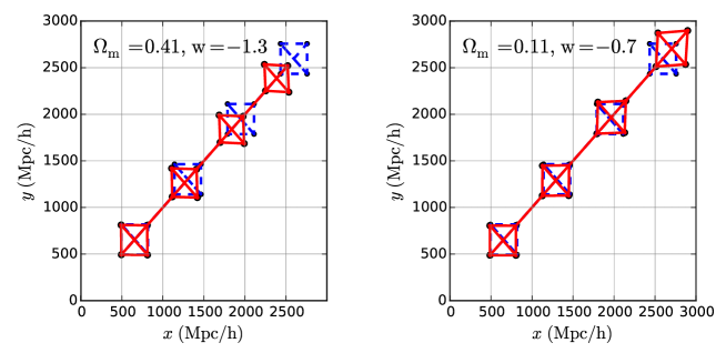
The Alcock-Paczynski (AP) test (Alcock & Paczynski, 1979) provides a geometric probe of $D_{A}$ and $H$. Given a certain cosmological model, the radial and tangential sizes of distance objects or structures can be computed as $\Delta r_{\parallel}=\frac{c}{H(z)}\Delta z$ and $\Delta r_{\bot}=(1+z)D_{A}(z)\Delta\theta$, where $\Delta z$, $\Delta\theta$ are the observed redshift span and angular size, respectively. When incorrect cosmological models are assumed for transforming galaxy redshifts into comoving distances, the wrongly estimated $\Delta r_{\parallel}$ and $\Delta r_{\bot}$ induces geometric distortion (see Figure 1). In galaxy redshift surveys, measuring the galaxy clustering in the radial and transverse directions enables us to probe the AP distortion, and thus place constraints on cosmological parameters (Ryden, 1995; Ballinger, Peacock & Heavens, 1996; Matsubara & Suto, 1996; Outram et al., 2004; Blake et al., 2011; Lavaux & Wandelt, 2012; Alam et al., 2016; Mao et al., 2016).

The main difficulty of AP test is that the radial distances of galaxies, inferred from their observed redshifts, are inevitably affected by the galaxy peculiar motions. This leads to apparent anisotropies in the clustering signal even if the adopted cosmology is correct. This effect, known as redshift-space distortions (RSD), is usually much more significant than the AP distortion, and is notoriously difficult to be accurately modeled in the statistics of galaxy clustering (Ballinger, Peacock & Heavens, 1996; Jennings et al., 2011).

As a complementary method to apply the AP test, Marinoni & Buzzi (2010) proposed to statistically study a large number of galaxy pairs and search for the deviation from a symmetric distribution of direction; however, since the peculiar velocity distorts the observed redshifts and changes the apparent tilt angles of galaxy pairs, this method is also seriously limited by RSD (Jennings et al., 2011). In an effort to minimize RSD contamination, the shape of void regions (Ryden, 1995; Lavaux & Wandelt, 2012) has also been proposed as an AP probe. This approach has the advantage that the void regions are easier to model compared with dense regions, but has limitations in that it utilizes only low density regions of the LSS, and requires large samples to attain statistical significances and achieve competitive constraints (Mao et al., 2016).

Recently, a novel method of applying the AP test by investigating the redshift dependence of the distortion was proposed by Li et al. (2014, 2015). The method is motivated by Park & Kim (2010), where the authors found adopting wrong set of cosmological parameters would produce redshift-dependent distortion in the LSS. Li et al. (2014, 2015) applied this idea to the AP test analysis. The authors found that, on one hand, the anisotropies produced by the RSD effect are, although large, maintaining a nearly uniform magnitude over a large redshift range; on the other hand, the degree of anisotropies produced by AP varies much more significantly. So they developed a method searching for the AP distortion from the redshift evolution of the anisotropies in LSS.

A consequence of reducing the RSD effect is that, by avoiding the complex modeling of galaxy position and velocity distributions, it becomes possible to use galaxy clustering on scales as small as 6-40 $h^{-1}$Mpc. In this region, there exists a large amount of clustered structures (Zhang et al., 2018); thus enables us to derive tight constraint on cosmological parameters. This large amount of information can hardly be utilized by other LSS statistical methods.

The first application of this AP method (hereafter the tomographic AP method) to observational data was performed in Li et al. (2016). The authors split the 1.13 million Sloan Digital Sky Survey (SDSS) Data Release 12 (DR12) galaxies into six redshift bins, measured their anisotropic 2PCFs, and quantified the redshift evolution of anisotropy. In combination with the datasets of Cosmic Microwave Background (CMB), type Ia supernovae (SNIa), baryon acoustic oscillations (BAO), and the $H_{0}$ measurements, the authors obtained $\Omega_{m}=0.301\pm 0.006,\ w=-1.054\pm 0.025$ in a flat universe with cold dark matter and constant EoS dark energy components (hereafter $w$CDM). The error bars are reduced by as much as 40% by adding the AP method into the combination of CMB+SNIa+BAO+$H_{0}$.

As a follow-up study, Li et al. (2018) improved the method by developing a technique accurately approximating the 2PCFs in different cosmologies. This greatly reduces the computational expense of the 2PCFs, thus enables the exploration of models with three or more parameters. Li et al. (2018) applied the method to constrain a model of dynamical dark energy EoS $w(z)=w_{0}+w_{a}\frac{z}{1+z}$ (hereafter $w_{0}w_{a}$CDM), and improved the Planck+BAO+SNIa+$H_{0}$ constraint on $w_{0}$-$w_{a}$ by as much as 50%. Furthermore, in a very recent work, Zhang et al. (2018) combined the tomographic AP method with the BAO measurements, and obtained a Hubble constant $H_{0}=67.78^{+1.21}_{-1.86}$ km s^-1 Mpc^-1 (2.26% precision). The inclusion of AP reduces the error bar by 32%.

As a newly developed technique, the tomographic AP method shows promising potential in constraining cosmological parameters. However, it is still far from becoming as mature as the BAO method. To summarize, the method needs to be improved in three aspects:

• We shall improve its methodology, by enhancing its statistical power, better understanding and estimating the systematical effects, and reducing the computational cost, etc.

• So far the method has only been used to constrain a limited set of parameters of $\Omega_{m}$, $w(z)$ and $H_{0}$. It is undoubtedly desirable to extend its application to more parameters and models.

• Given that there are many on-going and planned LSS surveys including DESI (Aghamousa et al., 2016), EUCLID (Laureijs et al., 2011), HETDEX (Hill et al., 2008)), it is necessary to forecast the constraining power when the method is applied to these surveys.

In this work we explored all these three issues. In Sec. 2, we showed that the methodology used in Li et al. (2014, 2015, 2016, 2018) neglected the correlations among different redshift bins, which leads to an over-estimation of statistical power and a large statistical fluctuation. We proposed a full covariance matrix approach to solve this problem and make the analysis statistically more perfect. In Sec. 3, we performed a comprehensive study on its constraints on a serious of cosmological parameters. In Sec. 4, we forecast the cosmological constraints expected from the DESI survey. Conclusions of our work are given in Sec. 5.

2. Data and Methodology

The data and methodology used in this work is similar to what used in Li et al. (2014, 2015, 2016, 2018), except that we more completely evaluate the statistical uncertainties.

2.1. Data

2.1.1 SDSS DR12 Galaxies

The Sloan Digital Sky Survey (York et al., 2000), as the currently largest spectroscopic galaxy survey, has obtained spectra for more than three million astronomical objects. This created the most detailed three-dimensional maps of the Universe ever made. BOSS (Baryon Oscillation Spectroscopic Survey) (Dawson et al., 2012; Smee et al., 2013), as a part of the SDSS-III survey (Eisenstein et al., 2011), has obtained spectra and redshifts of 1.37 million galaxies selected from the SDSS imaging, covering a sky region of 9 376 $\rm deg^{2}$ and a redshift span of $0.1\lesssim z\lesssim 0.75$. Its wide redshift coverage and large amount of galaxies makes it the best material for performing the tomographic analysis.

Following Li et al. (2016), we use the spectroscopic galaxy sample of SDSS-III BOSS DR12, containing the LOWZ catalogue at $0.1\lesssim z\lesssim 0.45$ and the CMASS catalogue covering $0.4\lesssim z\lesssim 0.7$ (Reid et al., 2016). For purpose of a tomographic clustering analysis, we split the sample into six, non-overlapping redshift bins of $0.150<z_{1}<0.274<z_{2}<0.351<z_{3}<0.430<z_{4}<0.511<z_{5}<0.572<z_{6}<0.693$ . The total number of galaxies used in the analysis is 1,133,326.

2.1.2 Horizon Run 4 mocks

We rely on the Horizon Run 4 (HR4; Kim et al., 2015) to estimate and correct the systematics. HR4 is a large N-body simulation with box size $L={3150}$ $h^{-1}$Mpc and number of particles $6300^{3}$, produced under the WMAP5(Komatsu et al., 2011) cosmological parameters $(\Omega_{b},\Omega_{m},\Omega_{\Lambda},h,\sigma_{8},n_{s})$ = (0.044, 0.26, 0.74, 0.72, 0.79, 0.96). Mock galaxy samples are then created using a modified version of the one-to-one correspondence scheme (Hong et al., 2016). Comparing the 2pCF of the mocks to the SDSS DR7 volume-limited galaxy sample (Zehavi et al., 2011), we found the simulated 2pCF shows a finger of god (FOG) feature (Jackson, 1972) rather close to the observation. The projected 2pCF agrees with the observation within 1$\sigma$ deviation on scales greater than 1 ${h^{-1}}$Mpc Hong et al. (2016).

2.1.3 MultiDark PATCHY mocks

We utilize the set of 2,000 MultiDark PATCHY mock catalogues (Kitaura et al., 2015) from the dark matter simulation to the covariance matrix. The MultiDark PATCHY mocks are produced using approximate gravity solvers and analytical-statistical biasing models, calibrated to the BigMultiDark N-body simulation (Klypin et al., 2016). The mock surveys can well reproduce the number density, selection function, survey geometry, and 2PCF measurement of the BOSS DR12 catalogues, and have been adopted in a series of works (see Alam et al., 2016, and references therein) to conduct clustering analysis of BOSS galaxies.

2.1.4 DESI galaxies

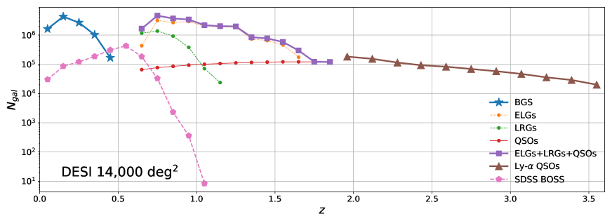
The DESI Aghamousa et al. (2016) observational program is a future project measuring the baryon acoustic feature of the large-scale structure, as well as the distortions effects of redshift space. DESI provides high precision measurements of the Universe’s expansion rate up to z $\sim$ 1.5. The baseline assumption is that it runs over an approximately five years period covering 14,000 deg² in area. The DESI survey makes observations of four types of objects:

• A magnitude-limited Bright Galaxy Survey (BGS)($0.05<z<0.45$) comprising approximately 10 million galaxies;

• Bright emission line galaxies (ELGs) (up to $z=1.65$) probing the Universe out to even higher redshift;

• Luminous red galaxies (LRGs) (up to $z=1.15$), which extend the BOSS LRG survey in both redshift and survey area;

• Quasi-stellar objects (QSOs) as direct tracers of dark matter in the redshift range $0.65<z<1.85$.

The number density distribution of these galaxies is shown in Figure 2. Our forecast in section 4. is based on these numbers.

2.2. Methodology

2.2.1 Quantifying the Anisotropy

Li et al. (2016) (hereafter Li16) split the BOSS DR12 galaxies into six redshift bins, and computed the integrated 2pCF in each bin

$$\xi_{\Delta s}(\mu)\equiv\int_{s_{\rm min}}^{s_{\rm max}}\xi(s,\mu)\ ds,$$ (1)

where the correlation function $\xi$ is measured as a function of $s$, the distance separation of the galaxy pair, and $\mu=\cos(\theta)$, with $\theta$ being the angle between the line joining the pair of galaxies and the line of sight (LOS) direction to the target galaxy. The range of integration was chosen as $s_{\rm min}=6$ $h^{-1}$Mpc and $s_{\rm max}=40$ $h^{-1}$Mpc. By focusing on the redshift dependence of anisotropy, the RSD effect is largely reduced, and it becomes possible to use the galaxy clustering down to 6 $h^{-1}$Mpc.

To mitigate the systematic uncertainty from galaxy bias and clustering strength, Li16 further normalized the amplitude of $\xi_{\Delta s}(\mu)$ to focus on the shape, i.e.

$$\hat{\xi}_{\Delta s}(\mu)\equiv\frac{\xi_{\Delta s}(\mu)}{\int_{0}^{\mu_{\rm max}}\xi_{\Delta s}(\mu)\ d\mu}.$$ (2)

A cut $\mu<\mu_{\rm max}$ is imposed to reduce the fiber collision and FOG effects.

2.2.2 The Redshift Evolution of Anisotropy

The redshift evolution of anisotropy, between the $i$th and $j$th redshift bins are be quantified as

$$\delta\hat{\xi}_{\Delta s}(z_{i},z_{j},\mu)\ \equiv\ \hat{\xi}_{\Delta s}(z_{i},\mu)-\hat{\xi}_{\Delta s}(z_{j},\mu),$$ (3)

where the systematics of $\delta\hat{\xi}_{\Delta s}$ (hereafter $\delta\hat{\xi}_{\Delta s,\rm sys}$), mainly comes from the redshift evolution of RSD effect , was measured from the Horizon Run 4 (Kim et al., 2015) N-body simulation and subtracted.

2.2.3 “Part-cov” approach of likelihood

To quantify the overall redshift evolution in the sample, Li16 chose the first redshift bin as the reference, compare the measurements in higher redshift bins with it, and then sum up these differences. So we have the following $\chi^{2}$ function describing the total of evolution

$$\chi_{\rm AP,part-cov}^{2}\equiv\sum_{i=2}^{6}\sum_{j_{1}=1}^{n_{\mu}}\sum_{j_{2}=1}^{n_{\mu}}{\bf p}(z_{i},\mu_{j_{1}})({\bf Cov}_{i}^{-1})_{j_{1},j_{2}}{\bf p}(z_{i},\mu_{j_{2}}),$$ (4)

where $n_{\mu}$ denotes the binning number of $\hat{\xi}_{\Delta s}(\mu)$, and ${\bf p}(z_{i},\mu_{j})$ is defined as

$${\bf p}(z_{i},\mu_{j})\equiv \ \delta\hat{\xi}_{\Delta s}(z_{i},z_{1},\mu_{j})-\delta\hat{\xi}_{\Delta s,\rm sys}(z_{i},z_{1},\mu_{j}).$$ (5)

The covariance matrix ${\bf Cov}_{i}$ is estimated from the 2,000 MultiDark-Patchy mocks (Kitaura et al., 2015). In wrong cosmologies, the AP effect produces large evolution of clustering anisotropy, thus would be disfavored due to a large $\chi^{2}$ value.

In Eq.4 we labeled the $\chi^{2}$ function by the $\chi^{2}$ analysis by “part-cov”, to denote that this $\chi^{2}$ analysis does not include the correlations among different ${\bf p}(z_{i})$s. The different ${\bf p}(z_{i})$s are actually correlated with other, in the sense that 1) since all the ${\bf p}(z_{i})$s takes the first redshift bin as the reference, the fluctuation in the first bin enters all ${\bf p}(z_{i})$s and makes them statistically correlate with each other; 2) the LSS at different redshift bins have correlations even if they are not overlapping with each other (galaxies lying near the boundary of a redshift bin have been affected by galaxies in the both nearby bins in the past structure formation era).

We tested and found ignoring 2) does not lead to significant changes in the results, so it is a minor effect. But ignoring 1) leads to $\sim$20% mis-estimation of the statistical error. The “part-cov” method relies on the first redshift bin as the reference. If this bin happened to have a large deviation (i.e. due to statistical fluctuation) from its statistical expectation, then all ${\bf p}$s would be affected. This creates statistical error in the results, which haven’t been included in Li et al. (2016, 2018).

Appendix A shows the mis-estimation and large fluctuation of this part-cov approach. They would be overcome if we include the correlations among the ${\bf p}(z_{i})$s into the analysis.

2.2.4 “Full-cov” approach of likelihood

We adopt the following formula to represent the $\chi^{2}$ function including all correlations,

$$\chi_{\rm AP,full-cov}^{2}\equiv{\bf P}\cdot{\bf Cov}\cdot{\bf P},$$ (6)

where

$${\bf P}=({\bf\tilde{p}}(z_{2},\mu_{j_{1}}),...,{\bf\tilde{p}}(z_{6},\mu_{j_{1}})),$$ (7)

a vector containing $(n_{z}-1)\times(n_{\mu})$ components, is built by joining all ${\bf\tilde{p}}(z_{i},\mu_{j})$s together. Here we re-define the $\bf p$ as the evolution between the nearby redshift bins, i.e.

$$\tilde{\bf p}\equiv\ \delta\hat{\xi}_{\Delta s}(z_{i},z_{i-1})-\delta\hat{\xi}_{\Delta s,\rm sys}(z_{i},z_{i-1}).$$ (8)

Actually, the results does not change if we still use the original $\bf p$ defined in Eq(5) . We redefine $\bf p$ as $\bf\tilde{p}$ so that the formula explicitly has no special redshift bin chosen as the reference.

Figure 3.— The covariance matrix of the $\hat{\xi}_{\Delta s}(z_{i},z_{i-1})$s (upper panel), and its normalized version (i.e. correlation coefficients, lower panel) We split each $\hat{\xi}_{\Delta s}(z_{i},z_{i-1})$ into 20 bins in the $\mu$ space, so five of them form a 100$\times$100 covariance matrix. The five 20$\times$20 matrices at the diagonal are the auto-correlations, while the off-diagonal matrices describe the cross-correlation. The non-zero cross-correlation, especially between the $\hat{\xi}_{\Delta s}(z_{i},z_{i-1})$s next to each other, suggests the necessity of including them into the analysis. See Section 2.2.4 for details.

2.2.5 The covariance matrix

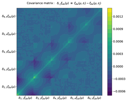
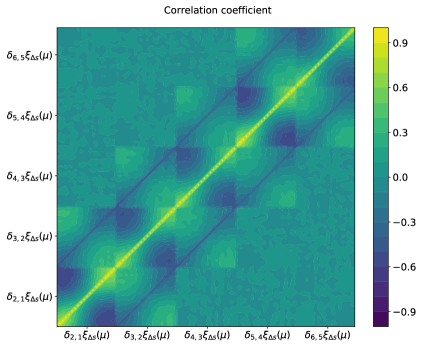
The covariance matrix $\bf Cov$, estimated from the MultiDark mocks, was shown in the Figure 3. The upper panel shows the covariance matrix when we split $\xi_{\Delta s}$ into 20 bins in $\mu$ space, while the lower panel shows the normalized covariance matrix (i.e. the correlation coefficient).

We find:

• Since we have 6 redshift bins, in total we need 6-1=5 $\delta_{i,j}\xi_{\Delta s}$s to characterize the evolution among them. So the plot of total covariance matrix contains 5$\times$5=25 regions of “cells”.

• The five “diagonal cells” describe the $20\times 20$ auto covariance matrix of $\delta_{i,j}\xi_{\Delta s}(\mu)$. $\mu$-bins close to each other strong positive correlations, while $\mu$-bins very far away from each other have negative correlations imposed by the normalization condition.

• The 20 “non-diagonal boxes” describe the cross-correlation among different $\delta_{i,j}\xi_{\Delta s}$s. They have non-zero values.

• Those $\delta_{i,j}\xi_{\Delta s}$s who have overlapping redshift bins are strongly correlated since they contain the same $\xi_{\Delta s}(\mu,z_{i})$ (e.g., $\delta_{2,1}\xi_{\Delta s}$ and $\delta_{3,2}\xi_{\Delta s}$ both depend on the $\xi_{\Delta s}$). Their pattern of correlation is similar to the diagonal boxes, i.e. positive correlation among nearby $\mu$-bins and negative among very faraway $\mu$-bins.

• $\delta_{i,j}\xi_{\Delta s}$s without any overlapping bins do not show significant cross-correlations (correlation coefficients close to 0). We tested and found that, ignoring them does not have statistically significant impact on the derived cosmological constraints.

3. Cosmological Constraints

The cosmological constraints are derived from the likelihood method described in Sec. 2.2. We divide our discussion into two sections. In Sec. 3.1 we presented the constraints on the background parameters of $w$, $w_{0}$, $w_{a}$, $\Omega_{m}$ and $H_{0}$, within the framework of $\Lambda$CDM, $w$CDM and $w_{0}w_{a}$CDM models, respectively. These parameters are directly constrained by the AP method, which measures the geometry of the universe in the late-time expansion era . In Sec. 3.2, we extend the scope and explore the other cosmological parameters, including the $\Lambda$CDM parameters and their derivations, and the 1-parameter extensions to $\Lambda$CDM and $w$CDM models.

We present the cosmological constraints when the AP likelihood is combined with several external datasets, including the full-mission Planck observations of CMB temperature and polarization anisotropies (Ade et al., 2015), the BAO distance priors measured from SDSS DR11 (Anderson et al., 2013), 6dFGS (Beutler et al., 2011) and SDSS MGS (Ross et al., 2015), the “JLA” SNIa sample (Betoule et al., 2014), and the Hubble Space Telescope measurement of $H_{0}=70.6\pm 3.3$ km/s/Mpc (Riess et al., 2011; Efstathiou, 2014). They are exactly the same datasets used in Li et al. (2016, 2018).

Table 1Mean values and 68% confidence limits of cosmological parameters for the $\Lambda$CDM, $w$CDM and $w_{0}w_{a}$CDM models, from combinations of Planck+BAO and Planck+BAO+AP. The uncertainties (of the last 2 digits of the numbers) are listed in the brackets.

$$\Omega_{\rm m} H_{0} w_{0} w_{a} \Lambda{\rm CDM} \ \ 0.3102(64)\ \ \ \ 0.3041(67)\ \ \ \ 67.63(48)\ \ \ \ 68.08(52)\ \ w{\rm CDM} 0.306(13) 0.293(10) 68.3\pm 1.5 69.8\pm 1.2 -1.031(63) -1.090(47) w_{0}w_{a}{\rm CDM} 0.351(29) 0.300(17) 64.0\pm 2.7 69.3\pm 1.7 -0.51(30) -0.95(18) -1.47(83) -0.53(53)$$ Model Planck+BAO +AP Planck+BAO +AP Planck+BAO +AP Planck+BAO +AP . . .

3.1. Constraints on background parameters

Table 1 summarizes the Planck+BAO and Planck+BAO+AP constraints on the background parameters $w$, $w_{0}$, $w_{a}$, $\Omega_{m}$ and $H_{0}$, within the framework of $\Lambda$CDM, $w$CDM and $w_{0}w_{a}$CDM models. In what follows, we discuss about them in details.

3.1.1 $\Lambda$CDM parameters

The $\Lambda$CDM model with EoS $w_{\Lambda}=-1$ is the simplest candidate among a large number of dark energy models, with the Hubble parameter taking form of

$$H(z)=H_{0}[\Omega_{m}(1+z)^{3}+\Omega_{\Lambda}]^{1/2},$$ (9)

where $\Omega_{m}+\Omega_{\Lambda}=1$ (we neglect curvature and radiation). Although $\Lambda$CDM model seriously suffers from the theoretical fine tuning and coincidence problems (Weinberg, 1989), it is in good agreement with most of the current observational data (Li et al., 2011).

Table 1 list the constraints on $\Omega_{m}$, $H_{0}$ derived from Plank+BAO and Plank+BAO+AP, respectively. Including AP into the analysis leads to a $\lesssim 1\sigma$ shift in the central values of $\Omega_{m}$, $H_{0}$, i.e. from (0.310,67.6) to (0.304,68.1), respectively.

3.1.2 $w$CDM parameters

Figure 4.— Cosmological constraints within the framework of $w$CDM. Upper panel: the constraint on $w$ from the combinations of Planck+BAO, Planck+BAO+AP, Planck+BAO+SNIa+$H_{0}$+AP. Lower panel: likelihood contours (68.3 and 95.4% CL) in the $\Omega_{m}$-$w$ plane.

Figure 5.— Cosmological constraints for $w_{0}w_{a}$CDM model. Upper panel: likelihood contours (68.3 and 95.4%) in the $\Omega_{m}$-$w$ plane. Adding AP into Planck+BAO greatly improves the constraints on the $w_{0}-w_{a}$ parameters. Low panel: evolution of $w(z)$ in the 68.3 and 95.4% CLs. A dynamical dark energy crossing $w=-1$ is mildly favored $\sim 1.5\sigma$ CL.

The simplest generalization to $\Lambda$ is considering a constant dark energy EoS $w$, and the Hubble parameter is given by

$$H(z)=H_{0}[\Omega_{m}(1+z)^{3}+\Omega_{de}(1+z)^{3(1+w)}]^{1/2},$$ (10)

where $\Omega_{de}$ is the current value of the dark energy density. If $w=-1$, then $w$CDM reduces to $\Lambda$CDM, with $\Omega_{de}=\Omega_{\Lambda}$.

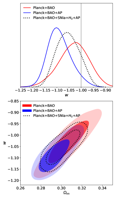
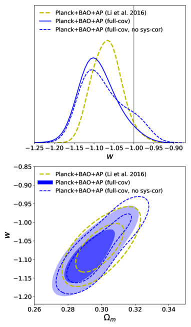
The upper panel of Figure 4 illustrates the constraint on $w$ from the combination of Planck+BAO, Planck+BAO+AP, Planck+BAO+SNIa+$H_{0}$+AP. The mean values as well as the 68% and 95% limits are

$$w =-1.031\ ^{+0.067}_{-0.057}\ {}^{+0.117}_{-0.130}\ \ {\rm Planck+BAO};$$ (11)

$$w =-1.089\ ^{+0.040}_{-0.054}\ {}^{+0.104}_{-0.088}\ \ {\rm\ +AP};$$ (12)

$$w =-1.054\ ^{+0.046}_{-0.052}\ {}^{+0.090}_{-0.085}\ \ {\rm\ +SNIa+}H_{0}{\rm+AP}.$$ (13)

If we describe the decrement in the error bar (or equivalently, improvement in the precision) by $\frac{\sigma_{\rm w.o.\rm AP}-\sigma_{\rm with\ AP}}{\sigma_{\rm w.o.\ AP}}$, then adding AP into the Planck+BAO combination reduces the errors by $\sim$30%. The inclusion of AP also shifts the constraint toward negative EoS by $\sim$1$\sigma$, making the results marginally consistent with $w=-1$ in 2$\sigma$. Further adding the SNIa and $H_{0}$ “pulled back” it towards $w=-1$.

The lower panel of Figure 4 shows the marginalized constraint in the $\Omega_{m}$-$w$ plane. We see a positive degeneracy between the two parameters, and a shift of $w$ towards negative values. Correspondingly, a smaller amount of $\Omega_{m}$ is preferred.

It is commonly believed that since the CMB data helps the BAO method to determine the absolute value of the sound horizon, tight constraints can be achieved if the two combined. So we will use Planck+BAO as a “standard combination” and check how much the constraints improve after adding AP. In fact, because CMB and AP constrain different epochs of expansion history, combining them can also effectively reduce the uncertainties of parameters. This can be seen from Figure 10 of Li et al. (2016), where we find the Planck and AP contours have orthogonal directions of degeneracy in the $\Omega_{m}$-$w$ space. Actually, combining these two constrains give

$$\Omega_{m}=0.295\pm 0.015,\ H_{0}=69.7\pm 1.7,\ w=-1.08\pm 0.05,$$ (14)

which are as tight as the Planck+BAO results.

The derived constrained from the full-covmat analysis is consistent with Li et al. (2016) except that here we obtained a larger error bar, mainly due to the inclusion of full covariance. A comparison between the two sets of results are presented in Appendix Appendix B: Robustness Check.

To ensure the robustness of the results, we have conducted a serious checks about the systematics and the options of the AP analysis. We do not find any statistically significant effect on the derived results. These tests are briefly discussed in Appendix Appendix B: Robustness Check.

3.1.3 $w_{0}w_{a}$CDM parameters

We move on to a further generalization and consider a dynamical EoS depend on $z$. As a simplest parameterization widely used in the literature, one can consider the 1st order Taylor expansion of $w_{de}$ with respect to $(1-a)$, i.e.

$$w_{de}(z)=w_{0}+w_{a}(1-a)=w_{0}+w_{a}\frac{z}{1+z},$$ (15)

which is the well-known Chevallier-Polarski-Linder (CPL) parameterization proposed by Refs. Chevallier & Polarski (2001); Linder (2003). The Hubble parameter is

$$H(z)=H_{0}[\Omega_{m}(1+z)^{3}+\Omega_{de}(1+z)^{3(1+w_{0}+w_{a})}e^{-3\frac{w_{a}z}{1+z}}]^{1/2}.$$ (16)

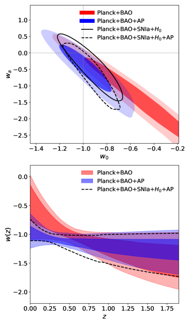
Figure 5 shows the constraints on this dynamical dark energy model. The Planck+BAO combination can not lead to effective constraints on the $w_{0}$-$w_{a}$ parameters. We only obtain two weak bounds of $w_{0}>-1.2,\ w_{a}<0.5$ (95%), and the upper bound of $w_{0}$ and lower bound of $w_{a}$ is left unconstrained. Adding AP closes the constraints and yields to

$$w_{0}=-0.95\ ^{+0.13}_{-0.18}\ {}^{+0.35}_{-0.35},$$

$$w_{a}=-0.53\ ^{+0.57}_{-0.43}\ {}^{+1.08}_{-1.17}\ \ {\rm Planck+BAO+AP}.$$ (17)

The result is consistent with $w(z)=-1$ in 1$\sigma$. This manifests the power of AP method. Combining it with BAO significantly increases the amount of information extracted from the LSS data, and greatly tightens the dark energy constraint.

When further considering the SNIa and $H_{0}$ datasets, we find

$$w_{0}=-0.94\ ^{+0.11}_{-0.11}\ {}^{+0.22}_{-0.21},$$

$$w_{a}=-0.38\ ^{+0.45}_{-0.39}\ {}^{+0.82}_{-0.87}$$

$$\ \ \ ({\rm Planck+BAO+SNIa+}H_{0});$$ (18)

$$w_{0}=-0.93\ ^{+0.09}_{-0.10}\ {}^{+0.20}_{-0.18},$$

$$w_{a}=-0.65\ ^{+0.45}_{-0.40}\ {}^{+0.83}_{-0.88}$$

$$\ \ \ ({\rm Planck+BAO+SNIa+}H_{0}{\rm+AP}).$$ (19)

The main effect of adding AP is a $\approx$0.7$\sigma$ shift of $w_{a}$ towards negative values (which can be seen evidently from the upper panel of Figure 5). As a result, a dynamical dark energy (i.e., $w_{a}\neq-1$) is preferred at $\approx 1.5\sigma$. The lower panel of the Figure shows that, the dark energy EoS is evolving from $<-1$ to $>-1$ from high redshift epoch to the present. $w=-1$ is consistent with the constraint at $2\sigma$ CL .

3.2. Constraints on the other cosmological parameters

3.2.1 $\Lambda$CDM parameters

Table 2 Mean values and 68% confidence limits of cosmological parameters for the base $\Lambda$CDM model from Planck+BAO and Planck+BAO+AP combinations. The uncertainties (of the last 2 digits of the numbers) are listed in the brackets.

$$\Lambda$$CDM

Parameter Planck+BAO +AP

.

.

.

.

.

.

.

.

.

.

.

.

.

.

.

.

.

.

.

.

.

.

.

.

.

.

.

Table 3 Constraints on 1-parameter extensions to the $\Lambda$CDM and $w$CDM models, for combinations of Planck+BAO and Planck+BAO+AP. Note that we quote 95% limits here.

$$\Lambda$$CDM extension CDM extension

Parameter Planck+BAO +AP Planck+BAO +AP

.

.

.

.

.

Figure 6.— 68% and 95% confidence regions on 1-parameter extensions of the base $\Lambda$CDM, for Planck+BAO (red) and Planck+BAO+AP (blue).

Figure 7.— 68% and 95% confidence regions on 1-parameter extensions of the $w$CDM, from Planck+BAO (red) and Planck+BAO+AP (blue).

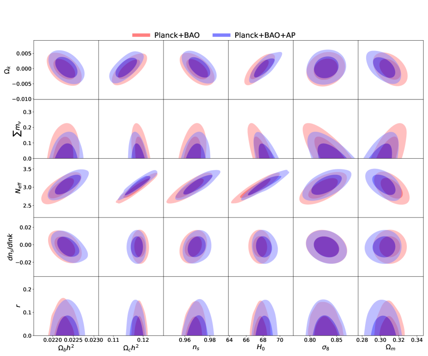
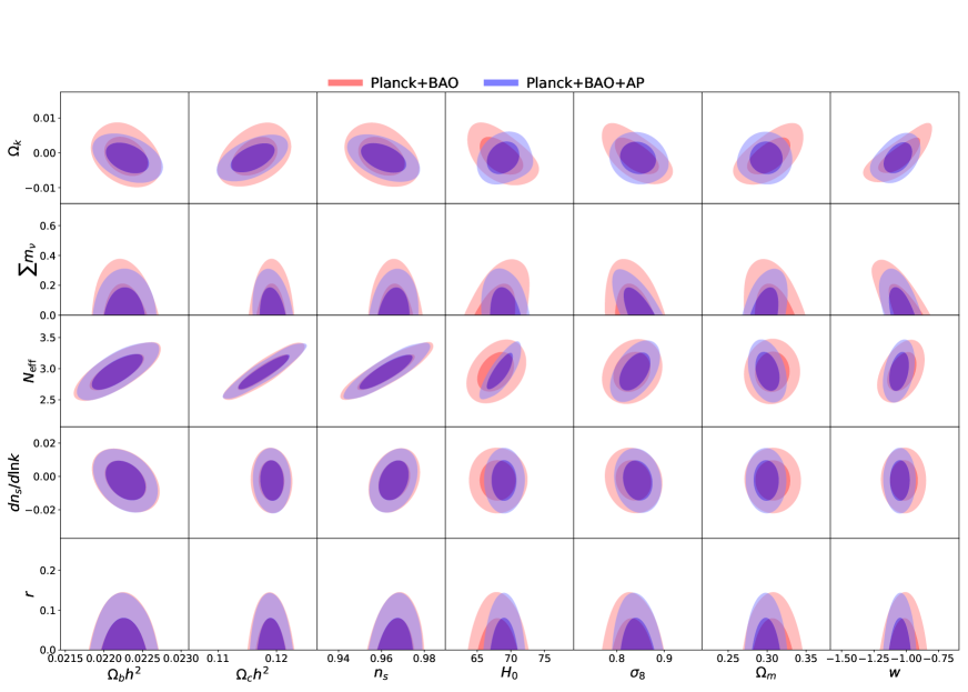
Table 2 summarizes the $\Lambda$CDM parameters (6 basic parameters, 21 derived; see Ade et al. (2015) for the explanation of their meanings) constrained by Planck+BAO and Planck+BAO+AP combinations.

In the $\Lambda$CDM framework, adding AP into the analysis only affects the constraint on $\Omega_{m}$. The matter amount $\Omega_{m}$ changes from $0.310$ to 0.304, which is a 1.0$\sigma$ CL drop (hereafter we use the Planck+BAO error bar to quantify the CLs of the changes). This then affects the constrains on many other parameters via the degeneracy among the parameters. For the basic parameters, we find :

• The cold dark matter density $\Omega_{c}h^{2}$ also decreases by 1.0$\sigma$.

• The baryon ratio $\Omega_{b}h^{2}$ is increased by 0.5$\sigma$, which should come from the increasing of $H_{0}$.

• The scalar spectral index $n_{s}$, which has negative degeneracy between $\Omega_{c}h^{2}$, is decreased by 0.7$\sigma$.

• The Thomson scattering optical depth due to reionization, $\tau$, and the log power of the primordial curvature perturbations, $\ln(10^{10}A_{s})$, has little degeneracy with the above parameters. So they are less affected (change < 0.3$\sigma$).

This leads to a serious of changes in the derived parameters:

• Due to the negative degeneracy between $\Omega_{m}$ and $H_{0}$, the latter increased by 0.9$\sigma$.

• $\sigma_{8}$ is negatively correlated with both $\Omega_{m}$ and $H_{0}$; as a net effect, its value remains unchanged.

• The acoustic scale $100\theta_{*}$, crucially determined by the CMB angular power spectrum measurement, remains less affected.

• The $z_{*}$ and $r_{*}$, affected by the density of energy components, are decreased and increased by 0.8$\sigma$; similar effects are found for $z_{\rm drag}$ and $r_{\rm drag}$.

• The change in $\Omega_{m}$ and $H_{0}$ leads to corresponding change in the combinations of $\Omega_{\Lambda}$, $\Omega_{m}h^{2}$, $\sigma_{8}\Omega_{m}^{0.5}$, and $\sigma_{8}\Omega_{m}^{0.25}$. The only exception is $\Omega_{m}h^{3}$; its value is almost fully determined by the acoustic scale $\theta_{*}$, so it remains unchanged.

• The age of the universe is rather sensitive to $\Omega_{m}$ and $\Omega_{\Lambda}$; we find it decreased by $0.7\sigma$.

• The matter-radiation equality redshift $z_{\rm eq}$ drops by 0.9$\sigma$, i.e. happens in latter epoch. It is due to the drop in $\Omega_{m}$ and increment in radiation density $\Omega_{r}$ (because of larger $h$).

• Affected by $z_{\rm eq}$ and the fraction of energy components, $k_{\rm eq}\equiv a(z_{\rm eq})H(z_{\rm eq})$ and $\theta_{s,\rm eq}\equiv r_{s}(z_{\rm eq})/D_{A}(z_{s}tar)$ (the comoving wavenumber of perturbation mode that entered Hubble radius at $z_{\rm eq}$, and the angular scale of the sound horizon at $z_{\rm eq}$) are also changed by 0.9$\sigma$.

• The characteristic wavenumber for damping $k_{\rm D}$ (which determines the photon diffusion length), whose value is related to the fraction of energy components, is slightly changed by 0.4$\sigma$.

• Parameters directly determined by $\tau$ and $A_{s}$, including $10^{9}A_{s}$, the parameter $10^{9}A_{s}e^{-2\tau}$ describing small-scale damping of CMB due to Thomson scattering at reionization, and the reionization redshift $z_{\rm re}$, all remain less affected.

3.2.2 1-Parameter Extensions to $\Lambda$CDM and $w$CDM

The Planck+BAO and Planck+BAO+AP constraint on other parameters of one-parameter extensions to $\Lambda$CDM and wCDM cosmology are given in Table 3. The determination of uncertainty listed in the table are at a confidence level of 95%.

In this case, adding AP into the combination decreases the value of $\Omega_{m}$, pulls the constrained region of $w$ to slightly negative values, and also reduces its error bar by 30%. This leads to evident effect on the curvature $\Omega_{k}$, the summation of neutrino mass $\sum m_{\mu}$, and the effective number of relativistic degrees of freedom in the Universe, $N_{\rm eff}$, via their degeneracies with $\Omega_{m}$ and $w$. The early universe parameters, such as the running $dn_{s}/d\ln k$ and the tensor-to-scalar ratio r, are less affected.

• Due to the degeneracy in their roles of governing the cosmic distances, $\Omega_{k}$ is negatively correlated with $\Omega_{m}$ and positively correlated with $w$. As shown in Table 3, after considering AP the absolute value of $\Omega_{k}$ increases (0.28$\sigma$) changes the sign form minus to plus for the $\Lambda$CDM extension model. For wCDM extension model, the absolute value of $\Omega_{k}$ becomes bigger (0.14$\sigma$), but the error is more tightly constrained (32% improvement).

• Using the AP effect the upper limit of the total neutrino mass are both reduced (by 22% and 18%) for $\Lambda$CDM extension and wCDM extension cases.

• By comparing two scenarios of Planck+BAO and Planck+BAO+AP datasets, $N_{\rm eff}$ is increased (0.6$\sigma$ for $\Lambda$CDM extension, not obvious in case of $w$CDM extension). The reduction in the error of $N_{\rm eff}$ is small (from 11.4% to 10.7% for $\Lambda$CDM extension, and from 12.7% to 12.1% for wCDM extension).

• The running of the spectral index $dn_{s}/d\ln k$ is typically small, while the error is not significantly changed in both cases.

• Adding the AP test, it appears that the tensor-to-scalar ratio $r$ is widely constrained for $\Lambda$CDM extension, and has tighter constraints for $\Lambda$CDM extension; but considering the statistical significance (0.05$\sigma$ and 0.02$\sigma$), the effect is really ignorable.

Figure 8.— Expected constraints on $w$CDM and $w_{0}w_{a}$CDM models from DESI survey. Combining AP with Planck+BAO breaks the degeneracy between parameters, so reduces the uncertainty of $w$ by 50%, and improving the $w_{0}$-$w_{a}$ constraint by a factor of 10.

The contour plots of one-parameter extensions to the $\Lambda$CDM model for combinations of Planck+BAO and Planck+BAO+AP are illustrated in Figure 6. We see clearly that combining the AP method increases the mean values of $N_{\mathrm{eff}}$, $\Omega_{b}h^{2}$, $n_{s}$, $H_{0}$, decreases $\Omega_{c}h^{2}$, $\Omega_{m}$, noticeably reduced the errors of $\Sigma m_{\nu}$.

The contour plots of one-parameter extensions to the $w$CDM model are illustrated in Figure 6. In this case adding AP helps sharpens the constraints $\Omega_{k}$, $\sum m_{\nu}$, $H_{0}$, $\sigma_{8}$, $\Omega_{\mathrm{m}}$, $w$ by 20-30%.

4. Forecast

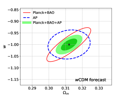
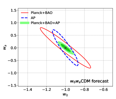
The number distribution of DESI galaxies is shown in Figure 2. Predicted constraints are made for the $w$CDM and $w_{0}w_{a}$CDM.

Estimating the covariance matrix of our correlation-based estimator is a complicated job (Bernstein, 1994; O’Connell et al., 2016). Among various terms that scale differently with $N_{gal}$, we found that

$${\bf Cov}\varpropto 1/N_{\rm gal},$$ (20)

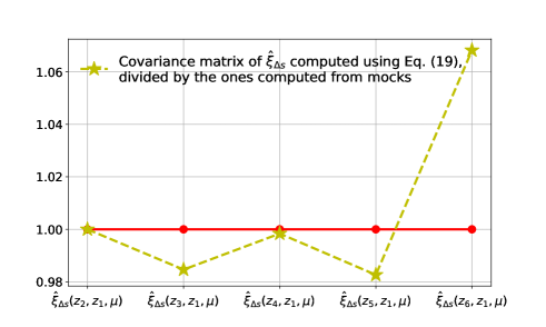
where $N_{\rm gal}$ is the number of galaxies, is already a good approximation. In Appendix Appendix B: Robustness Check we tested it using SDSS galaxies and find its error is $\lesssim 1.5\%-6\%$.

The DESI covariance matrices are then obtained simply using Eq. (20). Firstly, the covariance matrix of $\hat{\xi}_{\Delta s}(z_{2},z_{1},\mu)$ using SDSS galaxies are computed using the 2,000 MD-PATCHY mocks. We then choose this matrix as the baseline, take a ratio of the $N_{gal}$s of SDSS and DESI, and multiply this matrix by a factor to get the DESI covariance matrix .

The contour plot of $\Omega_{m}$ - $w$ in the wCDM model are illustrated at the top panel of Figure 8, using joint datasets of Planck+BAO, AP and Planck+BAO+AP, respectively. In the lower panels we show the contour plots of $w_{0}$ - $w_{a}$ in the frame of $w_{0}w_{a}$CDM model. In all cases we find that the constraint greatly reduced after adding the AP method.

For the constraint on a single parameter, the performance of AP and Planck+BAO are comparable to each other. If considering the joint constraint on two or more parameters, then the different directions of degeneracy from the two sets of results suggests that a greatly improved constraint can be achieved by combining them together.

In $w$CDM, adding AP reduces the constrained parameter space by 50%, achieving a precision of

$$\delta\Omega_{m}\approx 0.003,\ \delta w\approx 0.015\ (\rm Planck+DESI\ BAO+DESI\ AP).$$ (21)

In $w_{0}w_{a}$CDM, the addition of AP greatly reduces the constrained region by a factor of 10, achieving a precision of

$$\delta w_{0}\approx 0.035,\ \delta w_{a}\approx 0.11\ (\rm Planck+DESI\ BAO+DESI\ AP).$$ (22)

5. Concluding Remarks

We conduct a comprehensive study about the cosmological constraints derived from tomographic AP method. Based on Li et al. (2014, 2015, 2016, 2018), we improve the methodology by including the full covariance among clustering in all redshift bins. We then apply it to current and future observational data.

When applying it to current observational data, we find:

• The AP method noticeably improves the constraints on background evolution parameters $\Omega_{m}$, $H_{0}$, $w$, $w_{0}$, $w_{a}$. When combined it with the Planck+BAO the parameters’ error bars are reduced by $\sim 20-50\%$ (depends on the model and parameter).

• Using Planck+BAO+SNIa+$H_{0}$+AP, a dynamical dark energy $w_{a}\neq-1$ is preferred at $\approx 1.5\sigma$ CL.

• In the framework of $\Lambda$CDM, adding AP into Planck+BAO yields to a slightly smaller $\Omega_{m}=0.301\pm 0.010$, and a slightly larger $H_{0}=68.9\pm 1.2$. This leads to $\lesssim 1\sigma$ changes in $\Omega_{b}h^{2}$, $n_{s}$, $z_{*}$, $r_{*}$, $z_{re}$. $\tau$, $A_{s}$, $\sigma_{8}$ are less affected.

• When considering 1-parameter extensions to $\Lambda$CDM and $w$CDM models, we get improved constraints on $\Omega_{k}$, $\sum m_{\mu}$, $N_{\rm eff}$ when combining AP with Planck+BAO. Since AP only puts constraints on the late time expansion, early universe parameters $dn_{s}/d{\rm ln}k$ and $r$ are less affected.

We make a forecast of the $w$CDM and $w_{0}w_{a}$CDM constraints expected from Planck+DESI. We find the AP’s constraints on $\Omega_{m}$, $w$, $w_{0}$ and $w_{a}$ are as tight as the Planck+BAO ones, while the directions of degeneracy from the two differ from each other. Thus, combining them significantly improves the power of constraint. Adding AP reduces the error bar of $w$ by 50%, and improving the $w_{0}$-$w_{a}$ constraint by a factor of 10.

It should be pointed out that the many results presented in this work are not the optimistic ones. We expect the result being further improved with the improvement in the methodology, e.g. optimistic binning scheme of the galaxies, more aggressive clustering scales, more precise estimation of the covariance matrix, and so on.

According to our tests, for current surveys the systematic effects can not significantly affect the derived cosmological constraints. But it remains to be seen if this is true for future galaxy surveys. In particular, the systematic effects are estimated using one set of simulation performed in a fiducial cosmology, so the cosmological dependence of the systematics remains to be investigated in future works. It could be solved by, e.g. interpolating among systematics estimated from several sets of simulations with different cosmologies, considering theoretical estimation of systematics, and so on.

The tomographic AP method is so far the best method in separating the AP signal from the RSD distortions and using it we already achieved strong cosmological constraints. It is among the most powerful methods which can extract information from the $<$40 $h^{-1}\rm Mpc$ small-scale clustering region. It is essentially important for us to improving this method and preparing for its application to the next generation surveys.

Appendix A: The Full Covmat Method Compared with the Old Method

As described in Sec. 2, if one were ignoring the correlations between different $\delta_{i,j}\xi_{\Delta s}$s, and simply using Eq. 4 to calculate the $\chi^{2}$, the result suffers from two problems:

• The statistical power is over-estimated since part of the correlations are not considered;

• The result has a special dependence on the choice of the redshift bin (here the 1st bin), and thus suffers from large statistical fluctuation.

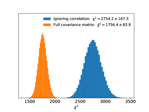
Here we conduct a simple test to see how large the above two effects are. We simply consider six independent variables obeying normal distribution, who share the same variance but have different mean values:

$$X_{i}\sim\mathcal{N}(\mu=10i,\sigma^{2}=1),\ i=1,2,3,4,5,6.$$ (23)

We then use the ideas of Eq. (4,6) to define a $\chi^{2}$ function characterizing the evolution among them:

$$\chi^{2}_{1} \equiv \sum_{i=2}^{6}(X_{i}-X_{1})^{2}/(\sigma^{2}+\sigma^{2}),$$ (24)

$$\chi^{2}_{2} \equiv \sum_{i=2}^{6}\sum_{j=2}^{6}(X_{i}-X_{1})\ {\bf Cov}_{i,j}\ (X_{j}-X_{1}),$$ (25)

and here the covariance matrix simply takes the form of

$${\bf Cov}_{ii}=2;\ {\bf Cov}_{ij}=1\ \rm for\ i\neq j.$$ (26)

We generate $10^{6}$ sets of $X_{i}$, compute their $\chi^{2}$ values, and plot the result in Figure 9. The mean and root-mean-square are listed in the legend. We find that

• In this case, the part-cov approach overestimates the $\chi^{2}$ value by 57%; i.e., it over estimates the statistical significance of the evolution.

• The statistical fluctuation of the $\chi^{2}$ derived from the part-cov approach is twice as large as the full-cov approach. This may lead to large bias when adopting this method to constrain cosmological parameters.

Figure 10 compares the Planck+BAO+AP constraint on $w$CDM derived using the 1st-bin approach Eq. (yellow dashed line) and the full-covmat approach (blue line). We find

$$w=-1.068\ ^{+0.036}_{-0.040}\ {}^{+0.076}_{-0.073}\ {\rm par-cov},$$ (27)

$$w=-1.089\ ^{+0.040}_{-0.054}\ {}^{+0.104}_{-0.088}\ {\rm full-cov}.$$ (28)

When using the full-covmat approach, the mean value was shifted towards the negative values by 0.02 ($\sim 0.4\sigma$), and the upper/lower error bars are enlarged by 10%/26%, respectively The two sets of results are, still, in statistical consistency. The errors due to the defect of the 1st-bin approach are not serious.

The part-cov constraint is weaker than what reported in Li et al. (2015) ($w=-1.054\pm 0.025$) because the difference in the choices of $n_{\mu}$ ((Li et al., 2015) adopted $n_{\mu}=6-40$ and here we reduced it to 20-25). Different from Li et al. (2015), in this work, we adopt the technique developed in Li et al. (2018) to efficiently approximate the 2PCFs in different cosmologies, and increase the size of covariance matrix from $n_{\mu}\times n_{\mu}$ to $5n_{\mu}\times 5n_{\mu}$. Both changes make the analysis more sensitive to the noise in the 2PCFS. So we reduce the number of binning to reduce the noise in $\xi_{\Delta s}$, which increase the reliability of the results, in the cost of scarifying some power of constraints.

Figure 9.— Histogram of $\chi^{2}$ values using six test variables as described in Section Appendix A: The Full Covmat Method Compared with the Old Method. The full covariance matrix method results in reliable and stable estimation of $\chi^{2}$s, while ignoring the covariance overestimates the $\chi^{2}$s and suffers from significantly larger uncertainty.

Figure 10.— $w$CDM. 1) The method we used in this paper (full covmat method) is different from Li et al. 2016 (where they do not use full covmat). Result is slightly different. 2) If we discard systematic correction (estimated from HR4 simulation), there is minor change in the results.

Figure 11.— $w$CDM. Plotted are 2$\sigma$ regions of parameters. If we change the options in the analysis, changes in the results are minor.

Figure 12.— A rough check of Eq. (20) using 6 bins of SDSS DR12 galaxies (see Figure 2 of Li16). The covariance matrices of $\hat{\xi}_{\Delta s}(z_{i},z_{1},\mu)$, $i=1,2,3,4,5$ are computed using two methods: 1. Measuring the scattering of $\delta_{i,j}$ from the 2,000 MultiDark-Patchy mocks, as we did in Li et al. (2016). 2. Measuring $\delta_{2,1}$ from the mocks, and infer the other $\delta_{i,j}$s simply using Eq. (20). The y-axis shows the ratio between the results of the two methods (method 2 over method 1). We find the estimation (method 2) achieve $<2\%$ precision for $\delta_{3,1}$, $\delta_{4,1}$, $\delta_{5,1}$. In the related redshift bins (redshift bins 1-5), the galaxy number density $\bar{n}_{\rm gal}$ varies in the range of $2-7\times 10^{-4}h^{-1}$ Mpc (as large as $\sim$3 times). Given such a large fluctuation of $\bar{n}_{\rm gal}$, Eq. (20) still achieves good precision. In the sixth bin $\bar{n}_{\rm gal}$ drops to significantly lower density ($1\times 10^{-4}(h^{-1}\rm Mpc)^{-3}$, $\sim$5 times lower than the first and second bins), while the error of method 2 is still $\lesssim$6%.

Appendix B: Robustness Check

Li16 tested the robustness of the tomographic AP method in details, and found the derived constraints on $w$CDM are insensitive to the adopted options within the range of $s_{\rm min}=2-8\ h^{-1}$ Mpc, $s_{\rm max}=30-50\ h^{-1}$ Mpc, $\mu_{\rm max}=0.85-0.99$, and number of binning $n_{\mu}=6-40$. Li et al. (2018) re-conducted the above tests in the $w_{0}w_{a}$CDM and obtained similar result. In what follows, we adopt the procedure of these two papers and test the robustness of the result. Our default set of options are $s_{\rm min}=6$ $h^{-1}$ Mpc, $s_{\rm max}=40\ h^{-1}$ Mpc, $\mu_{\rm max}=0.97$, and $n_{\mu}=15-20$ .

In the two panels of Figure 10 we also plotted the results without conduction any systematics (blue dashed). We see the peak value of $w$ remain almost unchanged; the only effect is a small ($\sim 10\%$ for the 95% contour) enlargement of constrained region towards the larger value of $w$ and $\Omega_{m}$. This is similar to what we found in Li et al. (2018), i.e. for the analysis of current observations the systematics effect is not large enough to result in a statistically significant change of the results.

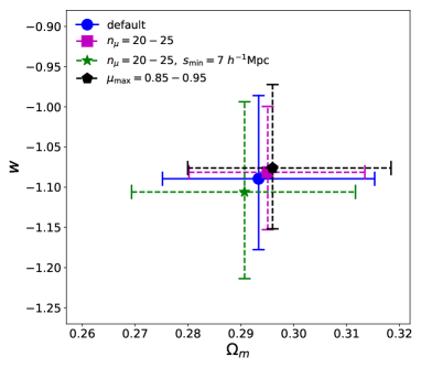
As a detailed test of the options adopted in the analysis, Figure 11 shows the mean values and 95% limits of the parameters, in cases of using a more aggressive binning scheme $n_{\mu}=20-25$, a more conservative small-scale cut $s_{\rm 7}=h^{-}1$Mpc, and a more conservative cut of correlation angle $\mu_{\rm max=0.85-0.95}$. In all cases we find rather small change in the mean values ($\lesssim 0.2\sigma$) and the limits ($\lesssim 15\%$). So we conclude the cosmological constraints obtained from the AP method does not sensitively depend on these options.

Finally, we test precision of Eq. 20 on the BOSS galaxies, and found it works with satisfying precision (Figure 12). The difference between the covariance matrices estimated from Eq. 20 and those directly computed using the mocks is $\lesssim$5%.

References

- Ade et al. (2015) Ade, P.A.R., Aghanim, N., & Arnaud, M., et al. arXiv:1502.01589
- Aghamousa et al. (2016) Aghamousa, A., 2016, arXiv:1611.00036
- Alam et al. (2016) Alam, S., Ata, M., & Bailey, S., et al. 2016, submitted to MNRAS (arXiv:1607.03155)
- Albrecht et al. (2006) Albrecht, A., Bernstein, G., & Cahn, R., et al. 2006. [astro-ph/0609591].
- Alcock & Paczynski (1979) Alcock, C., & Paczynski, B. 1979, Nature, 281, 358
- Anderson et al. (2013) Anderson, L., Aubourg, É., & Bailey, S. et al. 2014, MNRAS, 441, 24
- Ballinger, Peacock & Heavens (1996) Ballinger, W.E., Peacock, J.A., & Heavens, A.F. 1996, MNRAS, 282, 877
- Bernstein (1994) Bernstein, G. M. 1994, ApJ, 424, 569
- Betoule et al. (2014) Betoule, M., Kessler, R., & Guy, J., et al. 2014, A&A, 568, 32
- Beutler et al. (2011) Beutler, F., Blake, C., & Colless, M., et al. 2011, MNRAS, 416, 3017
- Blake et al. (2011) Blake, C., Glazebrook, K., & Davis, T. M., 2011, MNRAS, 418, 1725
- Chevallier & Polarski (2001) Chevallier, M., Polarski, D. 2001, Int. J. Mod. Phys. D, 10, 213
- Dawson et al. (2012) Dawson, K.S., Schlegel, D.J., & Ahn, C.P., et al. 2012, AJ, 145, 10
- Efstathiou (2014) Efstathiou, G. 2014, MNRAS, 440, 1138
- Eisenstein et al. (2011) Eisenstein, D.J., Weinberg, D.H., & Agolet, E., et al. 2011, AJ, 142, 72
- Hill et al. (2008) Hill, G. J., Gebhardt, K., Komatsu, E., et al. 2008, in Astronomical Society of the Pacic Conference Series, Vol. 399, Panoramic Views of Galaxy Formation and Evolution, ed. T. Kodama, T. Yamada, & K. Aoki, 115
- Hong et al. (2016) Hong, S.E., Park, C.,& Kim, J. 2016, ApJ, 823, 103
- Jackson (1972) Jackson, J., 1972, MNRAS, 156, 1
- Jennings et al. (2011) Jennings, E., Baugh, C.M., & Pascoli, S. 2011, MNRAS, 420, 1079
- Kim et al. (2015) Kim, J., Park, C., L’Huillier, B., & Hong, S. E. 2015, JKAS, 48, 213
- Kitaura et al. (2015) Kitaura, F.S., Rodrıíguez-Torres, S., Chuang, C.-H., et al. arXiv:1509.06400
- Klypin et al. (2016) Klypin, A., Yepes, G., Gottlober, S., Prada, F., & Hess, S. 2016, MNRAS, 457, 4340
- Komatsu et al. (2011) Komatsu, E., Smith, K. M., & Dunkley, J., et al. 2011, ApJS, 192, 18
- Laureijs et al. (2011) Laureijs, R., Amiaux, J., & Arduini, S., et al. 2011, arXiv:1110.3193
- Lavaux & Wandelt (2012) Lavaux, G., & Wandelt, B.D. 2012, ApJ, 754, 109
- Lewis & Bridle (2002) Lewis, A., & Bridle, S. 2002, Phys. Rev. D, 66, 103511
- Li et al. (2011) Li, M., Li, X.-D., Wang, S., & Wang, Y. 2011, Commun. Theor. Phys., 56, 525
- Li et al. (2014) Li, X.-D., Park, C., Forero-Romero, J., & Kim, J. 2014, ApJ, 796, 137
- Li et al. (2015) Li, X.-D., Park, C., Sabiu, C.G., & Kim, J. 2015, MNRAS, 450, 807
- Li et al. (2016) Li, X.-D., Park, C., & Sabiu, C.G., et al. 2016, ApJ, 832, 103
- Li et al. (2018) Li, X.-D., Sabiu, C.G., & Park, C., et al. 2018, ApJ, 856, 88
- Linder (2003) Linder, E.V. 2003, Phys. Rev. Lett., 90, 091301
- Mao et al. (2016) Mao, Q., Berlind, A.A., Scherrer, R.J., et al. 2016, submitted to ApJ
- Marinoni & Buzzi (2010) Marinoni, C., & Buzzi, A. 2010, Nature, 468, 539
- Matsubara & Suto (1996) Matsubara T., & Suto, Y. 1996, ApJ, 470, L1
- Miao et al. (2018) Miao H., & Huang Z., 2018, ApJ, 868, 20
- O’Connell et al. (2016) O’Connell, R., Eisenstein, D., Vargas, M., Ho, S., & Padmanabhan, N. 2016, MNRAS, 462, 3
- Outram et al. (2004) Outram, P.J., Shanks, T., Boyle, B.J., Croom, S.M., Hoyle, F., Loaring, N.S., Miller, L., & Smith, R.J. 2004, MNRAS, 348, 745
- Park & Kim (2010) Park, C., & Kim, Y.-R. 2010, ApJL, 715, L185
- Perlmutter et al. (1999) Perlmutter, S., Aldering, G., & Goldhaber, G., et al. 1999, ApJ, 517, 565
- Reid et al. (2016) Reid, B., Ho, S., & Padmanabhan, N., et al. 2016, MNRAS, 455, 1553
- Riess et al. (1998) Riess, A.G., Filippenko, A.V., & Challis, P., et al. 1998, AJ, 116, 1009
- Riess et al. (2011) Riess, A.G., Macri, L., & Casertano, S., et al. 2011, ApJ, 730, 119
- Ross et al. (2015) Ross, A.J., Samushia, L., & Howlett, C., et al. 2015, MNRAS, 449, 835
- Ryden (1995) Ryden, B.S. 1995, ApJ, 452, 25
- Smee et al. (2013) Smee, S.A., Gunn, J.E., & Uomoto, A., et al. 2013, AJ, 146, 32
- Weinberg (1989) Weinberg, S. 1989, Reviews of Modern Physics, 61, 1
- Weinberg et al. (2013) Weinberg, D.H, Mortonson, M.J., Eisenstein, D.J., et al. 2013, Physics Reports, 530, 87
- Yoo & Watanabe (2012) Yoo, J., & Watanabe, Y. 2012, International Journal of Modern Physics D, 21, 1230002
- York et al. (2000) York, D.G., Adelman, J., & Anderson, J.E., et al. 2000, AJ, 120, 1579
- Zehavi et al. (2011) Zehavi, I., Zheng, Z., & Weinberg, D.H., et al. 2011, ApJ, 736, 59
- Zhang et al. (2018) Zhang, X., Huang, Q.-G., & Li, X.-D., 2019, MNRAS, 483, 1655