Siamese Convolutional Neural Network for Sub-millimeter-accurate Camera Pose Estimation and Visual Servoing

Abstract

Visual Servoing (VS), where images taken from a camera typically attached to the robot end-effector are used to guide the robot motions, is an important technique to tackle robotic tasks that require a high level of accuracy. We propose a new neural network, based on a Siamese architecture, for highly accurate camera pose estimation. This, in turn, can be used as a final refinement step following a coarse VS or, if applied in an iterative manner, as a standalone VS on its own. The key feature of our neural network is that it outputs the relative pose between any pair of images, and does so with sub-millimeter accuracy. We show that our network can reduce pose estimation errors to 0.6 mm in translation and 0.4 degrees in rotation, from initial errors of 10 mm / 5 degrees if applied once, or of several cm / tens of degrees if applied iteratively. The network can generalize to similar objects, is robust against changing lighting conditions, and to partial occlusions (when used iteratively). The high accuracy achieved enables tackling low-tolerance assembly tasks downstream: using our network, an industrial robot can achieve 97.5% success rate on a VGA-connector insertion task without any force sensing mechanism.

I Introduction

Visual Servoing (VS), where images taken from a camera typically attached to the robot end-effector are used to guide the robot motions, is an important technique to tackle robotic tasks that require a high level of accuracy [1]. Recently, researchers have explored Deep Neural Networks (DNN) to implement VS [2, 3], with the hope that DNN can mitigate certain shortcomings of classical VS, such as reliance on manually-crafted features [1], or sensitivity to lighting conditions [4]. The main issue with the architecture proposed in [2] is that a new network has to be trained for each reference pose, which makes it unpractical for actual industrial settings. Meanwhile, the approach proposed in [3] has several-millimeter errors on synthetic data and even larger errors on real data, which is insufficient for low-tolerance industrial tasks.

Here we propose a new neural network for highly accurate camera pose estimation, which can be used as a final refinement step following a coarse VS or, if applied in an iterative manner, as a standalone VS on its own. The key feature of our neural network is that it outputs the relative pose between any pair of images (by contrast with [2]), and does so with sub-millimeter accuracy (by contrast with [3]). This is achieved by leveraging a Siamese architecture [5], which contains two branches of extractors (one per image). The features extracted from the two images independently in this manner are then compared at subsequent layers to achieve very high accuracy.

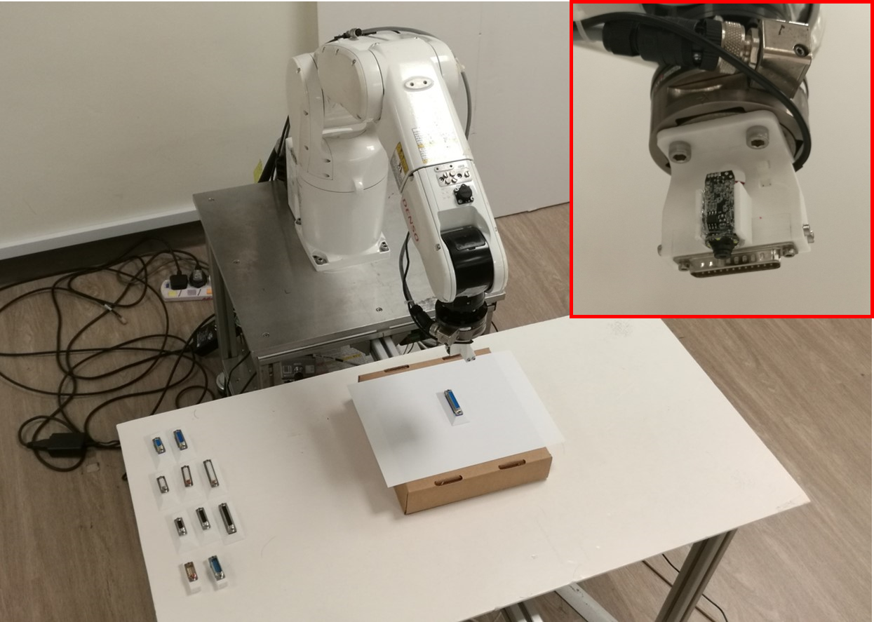
Figure 1: An industrial robot is used for the insertion experiments. The male connector is attached to the end-effector with the camera. A better view of the end-effector is placed at the top right corner.

More specifically, our main contributions are:

• our Siamese network can reduce initial errors of 10 mm in translation and 5 degrees in rotation to less than 0.6 mm in translation and 0.4 degrees in rotation, in a single shot;

• even though the network is trained with small pose differences ($\leq$10 mm in translation $\leq$5 degrees in rotation), it can deal with large initial errors (several cms in translation and tens of degrees in rotation) when used in an iterative manner, as a standalone VS solution, without any compromise in final accuracy;

• the high accuracy achieved enables tackling low-tolerance assembly tasks downstream: using our network, an industrial robot can achieve 97.5% success rate on a VGA-connector insertion task without any force sensing mechanism;

• our network can generalize to connectors it has never seen before, is robust against changing lighting conditions, and to partial occlusions (when used iteratively);

The paper is organized as follows. Section II discusses the related work, in both classical and Deep Learning-based Visual Servoing. Section III describes the network architecture in detail. Section IV explains the method used to automatically collect and accurately label the dataset used for training the model. Section V reports the experiment results, on the test set and in a physical VGA connector insertion task.

II Related Work

II-A Camera pose estimation

There has been a lot of research effort in camera pose estimation, which is crucial for vision-based robotic manipulation. A popular approach extracts feature points from two images, matches the corresponding features and determines the relative camera pose difference. Popular algorithms such as SIFT [6], DAISY [7], SURF [8] and ORB [9] are used in the local feature extraction and matching. However, the accuracy of the classical approach may suffer due to a scarcity of feature points found for matching.

In recent years, deep learning-based camera pose estimation has attracted the attention of the research community. The accuracy of deep learning-based camera pose estimation ranges from meters to centimeters on different datasets. In [10], researchers proposed a deep convolutional neural network with 2 m and 6° accuracy for large scale outdoor scenes and 0.5m and 10° for indoor scenes respectively. In both [11] and [12], the authors trained and tested the neural networks proposed in previous works on DTU dataset [13] which consists of images pairs of objects shot from different viewpoints, errors were reduced to a few centimeters.

However, most of these works were designed for tasks like simultaneous localization and mapping (SLAM) and visual odometry with relatively large workspace domain; few papers have discussed utilizing the robustness of deep learning for high precision camera pose estimation which is fundamental for industrial applications such as a fine assembly line.

II-B Deep learning-based Visual Servoing

Deep learning-based visual servoing often performs camera pose estimation iteratively while guiding the motion of the robot towards the target pose so as to achieve high final accuracy. In [3], researchers generated a Visual Servoing Scene Dataset (VSSD) by generating 5 simulated indoor scenes. Based on this dataset, flownet [14] achieved very good performance, reducing the error to a few millimeters.

In [2], an efficient way of generating dataset was proposed to train robust neural networks for visual servoing was proposed: by varying lighting conditions and adding random occlusions, a dataset could be produced within hours. The neural network trained on the dataset achieved sub-millimeter accuracy. However, the network was trained to estimate the camera pose difference between the current pose and a fixed reference pose by taking only one image captured at the current base. This essentially means a new network has to be trained for a new reference pose. In the same paper, another neural network which takes in two images was proposed as an extension. However, it could only achieve centimeter accuracy without adopting photometric visual servoing [15] at the last stage.

As pointed out by [16], the awareness of egomotion helps neural networks to learn features better. Therefore, in this paper, we propose a neural network with Siamese architecture and takes in two images from different viewpoints for high accuracy camera pose estimation.

III Neural Network

III-A Architecture

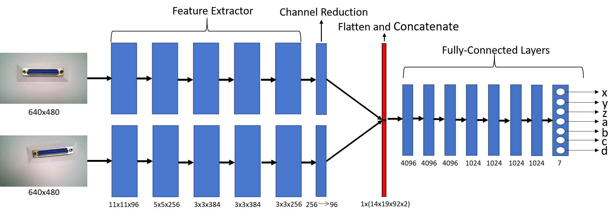
Figure 2: Neural network architecture.

Since the network was designed to output the transformation between two camera poses, it was intuitive to use a Siamese architecture (Fig 2) to extract features separately for the two input images. In contrast to [14], which concatenates two images along the channel axis and performs feature extraction, applying convolutions on the two images is likely to produce independent features for matching at a later stage. Each arm adopts the feature extractor of CaffeNet (referred by many as AlexNet) for its simplicity and proven effectiveness on the [17].

To control the number of parameters, a channel reduction layer is used to reduce channel from 256 to 96 with a convolutional kernel of size 1$\times$1.

We experimented many possible architecture designs for feature matching. Direct operation of summation or subtraction of the two feature maps from feature extractor has led to relatively poor performances. Inspired by [18], feature maps are flattened, concatenated and fed into the classifier, which is adopted from the Caffenet with minor adjustments to fit our input size. 5 additional fully connected layers are appended at the end to further improve the performance.

For output layers, we attempted a two-branch-in and two-branch-out architecture in order to estimate translations and rotations separately. However, low accuracy was resulted. It can be explained that the coupling effect of extrinsic parameters are significant and hence, the network should output translation and rotation parameters together, as in the final network design.

III-B Loss

Since we designed the network to estimate the relative transformation $T_{\Delta}$ between any two camera poses, not limiting to a fixed reference pose, an input pair is generated by collecting two samples, each consists of an image and a label $T_{d2e}$, which is the transformation from a default pose to the pose at which the image was taken (explained in greater details in the Dataset Generation and Training section). The images are marked as $I_{A}$ and $I_{B}$, the transformation label $T_{\Delta}$ is computed as:

$$T_{\Delta}=T_{d2e,A}\times T_{d2e,B}^{-1}$$

For brevity, the transformation label is decomposed into translation and rotation in terms of quaternions. The loss is then computed as:

$$L=\frac{1}{n}\sum_{i=1}^{n}wRMS(t_{i},{\hat{t}_{i}})+(1-w)RMS(q_{i},\hat{q}_{i})$$

where n is the number of input pairs, $t$ and $\hat{t}$ are translation label and estimation with the unit of meters, $q$ and $\hat{q}$ are rotation label and estimation in the form of normalized quaternions. Since the translation parameters are in meters, to balance the magnitude of values of translation and rotation parameters, a weight $w$ = 0.99 is used. $RMS$ is root-mean-square error defined as:

$$RMS(a,\hat{a})=\sqrt{\frac{1}{m}\sum_{j=1}^{m}(a_{j}-\hat{a}_{j})^{2}}$$

where m is number of parameters. For translation, m = 3 whereas for rotation, m = 4 due to quaternion representation.

We chose quaternions over Euler angles because the variable space of roll, pitch, and yaw is not a good representation of the actual rotation; quaternions are a better way to encode the axis-angle representation. This is also supported by experiments in some previous works such as [19].

IV Set-up

As shown in Figure 1, we designed and 3D printed an end-effector to be mounted at the tip of the robotic arm. A male connector can be mounted on the bottom of the end-effector. The corresponding female connector is mounted on a white frustum-shape base that is placed on a white A4-sized paper. The base is required as some connectors cannot stand on its own.

Clearly the base can provide some features for the network, however, we argue that the base can be regarded as part of the connector. In the actual production environment, there will always be additional features (such as other machine parts) in the scene other than the object of interest. We chose white as the color for the base and the background for two reasons: firstly, noise can be added easily to white pixels for data augmentation. Secondly, textureless background and base provide fewer features for the neural network to learn from so as to encourage the network to focus on the connectors.

An inexpensive (less than $20) short-range camera with the field of view 70 °and the resolution 640$\times$480, was installed on the side of the end-effector. The camera was equipped with 4 LED lights to improve lighting as the base was usually in the shadow of the robotic arm and the end-effector. We did not select an expensive high-resolution camera for three reasons: the model should not rely on high-resolution to reduce the cost of future industrial application; the neural network was designed to be light-weight so a small input size was preferred; the camera had to be small so it could be placed near the male connector such that the female connector could appear in its view at the insertion pose.

V Dataset Generation and Training

V-A Sample collection

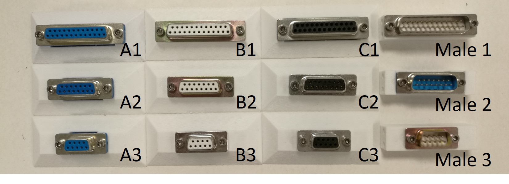
Figure 3: The female connectors come with different shapes (A: blue; B: white; C: black) and sizes (1,2 and 3); the male connectors of corresponding sizes are used.

Figure 3 shows the connectors used in the dataset and the experiments.

We guided the robotic arm to an insertion pose where the male connector mounted on the end-effector was inserted into the female connector on the base. Then the end-effector was lifted vertically for 15 cm to allow the camera to capture the full view of the connector with sufficient margins. The pose of the end-effector can be found by forward kinematics and was recorded as the default pose $T_{0}$. The default pose had its z-axis pointing vertically downwards if see from the world frame. Note that the default pose is not the reference pose mentioned in the experiments.

The entire collection process was automated and samples were generated by randomly changing the end-effector pose around the default pose. Since we were focusing on the last step of visual servoing, the sampling range of translation and rotation were small: the origin of new camera pose was uniformly sampled within a vertical cylinder with radius 5 mm and height 10 mm, with the default pose frame origin at the center of the bottom of the cylinder. The rotation was sampled uniformly from -5 degrees to 5 degrees for roll and pitch and -10 degrees to 10 degrees for yaw. An image taken by the camera and a corresponding pose (in the form of a transformation matrix from the default pose to the new end-effector pose $T_{d2e}$) were recorded for each arbitrary pose.

V-B Datasets

We firstly collected a small dataset with only the connector type A1 to verify the network’s robustness against changes in the lighting condition. Due to the shadows of the robotic arm and the end-effector, lighting was vastly different if the female connector is moved into the shadow. Rotation was also needed such that the shadows do not always appear at the same corner of a reference image. In addition, the reflection pattern on the female connectors were strongly affected by the position and the direction of the connector. In this dataset, we placed the female connector at 5 points on the workbench, with four spaced 5 cm in both x and y directions from each other forming the vertices of a square of, and the last one at the center of the square. On each point, we rotated the base 0°, 30°, 60°and 90°and for each orientation, 200 samples were collected, totalling $5\times 4\times 200=4000$ samples.

In addition, to enable generalization across different connectors with a single network, 1000 samples were collected for each of the 9 female connectors (A1, A2, … ,C3) to form a larger dataset. Further details are covered below.

V-C Training

For each connector, we took 50 samples each for validation and testing respectively, the rest was used for training. Note that for $n$ samples in each set, $n^{2}$ input pairs can be created. To prevent taking too much disk space, the input pair were created during training instead of being pre-processed.

We trained two models $M_{A1}$ and $M_{8}$. Model $M_{A1}$ was trained with only A1 ($M_{A1}$) for 10 epochs. A quarter of the maximum number of the training set, $3900^{2}\times 0.25=3802500$ input pairs were used in the training. The learning rate was $10^{-4}$ initially, and halved after the $4^{th}$, $6^{th}$ and $8^{th}$ epoch. Adam optimizer was used with $\beta_{1}=0.9$, $\beta_{2}=0.999$, $\epsilon=10^{-8}$ and no weight decay. The training was run on 4 GTX-1080Ti with a batch size of 256. Uniform weights initialization was applied.

Model $M_{8}$ was trained to evaluate the network’s ability to generalize across different connectors. We selected 8 connectors (all except A2) to form a dataset of $8\times 900^{2}=6480000$ input pairs for training. A2 was used in the experiment to verify the robustness of the network against a novel object.

VI Experiment Results

We evaluated the performance of models $M_{A1}$ and $M_{8}$ first on the test sets (as described in Sec. V-C) to obtain the mean errors of each parameter for a qualitative analysis of the model. After that, we tested the models on actual insertion tasks.

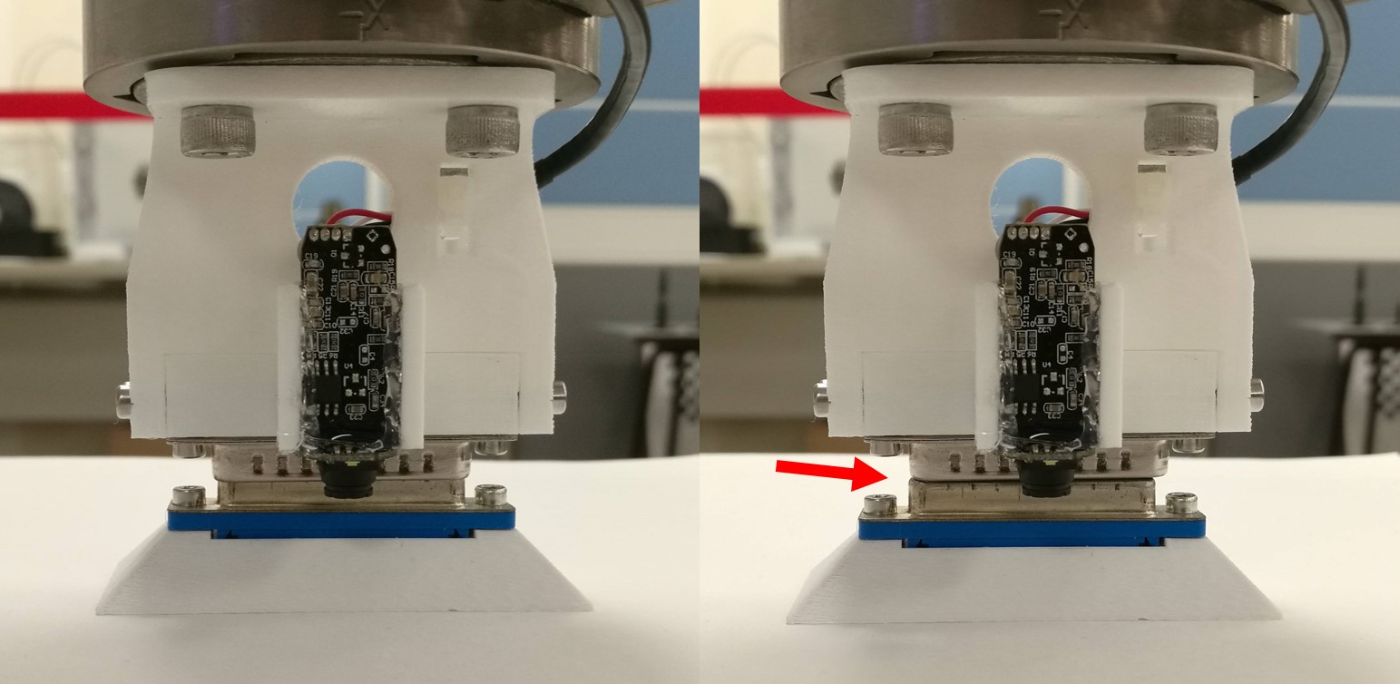
Figure 4: A successful (left) and an unsuccessful (right, collision point indicated by the red arrow) insertion.

As shown in Figure 4, an insertion is successful only if the male connector could completely go into the female counterpart. To evaluate the range of tolerances that allow successful insertions, we manually added offsets to the reference pose (the pose that results in a successful insertion) and tested the insertion. However, evaluating parameters separately (one at a time) is meaningless due to their coupled effect in the actual insertion. Hence, we clustered translation parameters (x, y, and z) and rotation parameters (roll, pitch, and yaw) separately into two groups. Each time we varied all parameters in a group by the same amount. To reduce the number of combinations, all offsets tested were positive. Table I was produced using connector A1. Note that this experiment was meant to allow readers to have a rough idea about the difficulty of the insertion; the coupled effect is much more complicated in the actual task.

It was observed that insertion of VGA connectors is indeed a challenging task: to achieve a successful insertion, a large error in certain parameters must be compensated by an extremely small error in other parameters.

TABLE I: Insertion tolerance analysis: a qualitative evaluation of the difficulty of the task. Note that these are not the insertion experiment results. Translation (x, y and z) and rotation (roll, pitch and yaw) parameters were clustered into two groups and the same offset was applied on parameters in the same group each time; A tick/cross indicates at that translation and rotation offsets, the insertion was successful/unsuccessful. For example, if x, y and z are all offset by +0.3 mm whereas roll, pitch and yaw are all offset by +1.00 degree, the insertion will be unsuccessful.

	0.0	0.1	0.2	0.3	0.4	0.5	0.6	0.7
0.00	✓	✓	✓	✓	✓	✓	✓	✕
0.25	✓	✓	✓	✓	✓	✓	✓	✕
0.50	✓	✓	✓	✓	✓	✕	✕	✕
0.75	✓	✓	✓	✓	✕	✕	✕	✕
1.00	✓	✓	✓	✕	✕	✕	✕	✕
1.25	✓	✓	✓	✕	✕	✕	✕	✕
1.50	✓	✓	✕	✕	✕	✕	✕	✕
1.75	✓	✓	✕	✕	✕	✕	✕	✕
2.00	✓	✓	✕	✕	✕	✕	✕	✕
2.25	✕	✕	✕	✕	✕	✕	✕	✕

VI-A Model trained on A1 ($M_{A1}$) for the evaluation of robustness against changes in the lighting conditions

VI-A1 Performance on the test set

the test set of A1 consists of $50^{2}=2500$ input pairs. The mean absolute errors of translation and rotation across the entire test set are tabulated in Table II. For easy interpretation, the quaternions were first converted to Euler angles for rotation error computation.

TABLE II: Errors of model $M_{A1}$ on the test set

Object	$\mathbf{e_{x}}$/mm	$\mathbf{e_{y}}$/mm	$\mathbf{e_{z}}$/mm	$\mathbf{e_{\phi}}$/°	$\mathbf{e_{\theta}}$/°	$\mathbf{e_{\psi}}$/°
A1	0.34	0.36	0.44	0.19	0.18	0.19

Notice that the mean translation errors were below 0.5 mm; the mean rotation errors were smaller than 0.2 degree. In the experiments, rotation affected the view of the camera more than translation did, hence there was no surprise that the network could learn to estimate the rotation extremely well. The errors in translation were more subtle, yet the network could still give reasonably good translation estimations.

VI-A2 Performance on actual insertion

For the actual insertion experiment, we firstly adjusted the robotic arm and the base such that if the end-effector went vertically downwards, the male connector could fully go into the female connector. An image $I_{ref}$ was then captured. Note that $I_{ref}$ was taken only once at the start of the experiment.

We then manually shifted (with rotation) the female connector on the workbench slightly and let a second image $I_{test}$ to be taken. The network took in $I_{ref}$ as $I_{A}$ and $I_{test}$ as $I_{B}$ and output 7 parameters to construct a transformation matrix $T_{\Delta}$.

Afterwards, the robot was moved to $T_{est}$ which is obtained as:

$$T_{est}=T_{\Delta}\times T_{test}$$

If the estimation was perfect, the connector in the third image $I_{est}$ taken would look identical as the connector in $I_{ref}$.

The end-effector is then descended blindly to attempt the insertion: no any other intermediate adjustments or corrections were performed. To expedite experiment, we did not apply further force to achieve a firm connection between the two connectors. Once the male connector fully went into the female connector, it was counted as a successful attempt. If the male connector got stuck at the rim of the female connector, it was counted as unsuccessful.

We repeated the above steps 50 times and the results are tabulated in III. Due to the displacement of the female connector, $I_{test}$ could be different from $I_{ref}$ in terms of lighting conditions due to shadows and the difference between $I_{ref}$ and $I_{test}$ could become larger and larger since $I_{ref}$ was constant. Yet, the network was able to catch up with the movement and performed most of the insertion correctly.

TABLE III: Performance of model $M_{A1}$ on actual insertion

	#Success	#Total Attempts	Percentage(%)
A1	47	50	94

VI-B Model trained on 8 connectors ($M_{8}$) for the evaluation of robustness against a novel connector

VI-B1 Performance on the test set

Similar to experiments conducted on $M_{A1}$, we fed the trained model $M_{A1}$ with the test set which consists of $8\times 50^{2}=20000$ input pairs. Results are tabulated in Table IV and Figure 5.

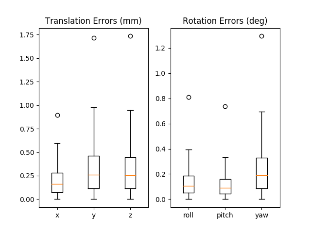
(a) Distributions of translation errors and rotation errors represented by box plots for the 8 connectors. The maximum outliers are drawn as circles on the top. The five horizontal lines from top to bottom indicate the maximum fence, the third quartile, the mean value, the first quartile and the minimum fence.

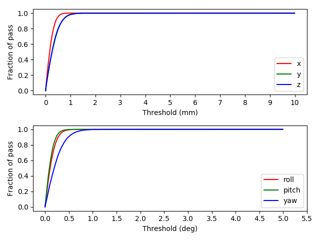
(b) Percentage of pass vs threshold curves for the 8 connectors. Top: translation errors; bottom: rotation errors. The graph shows the percentage of test pair with error lower that the corresponding threshold values.

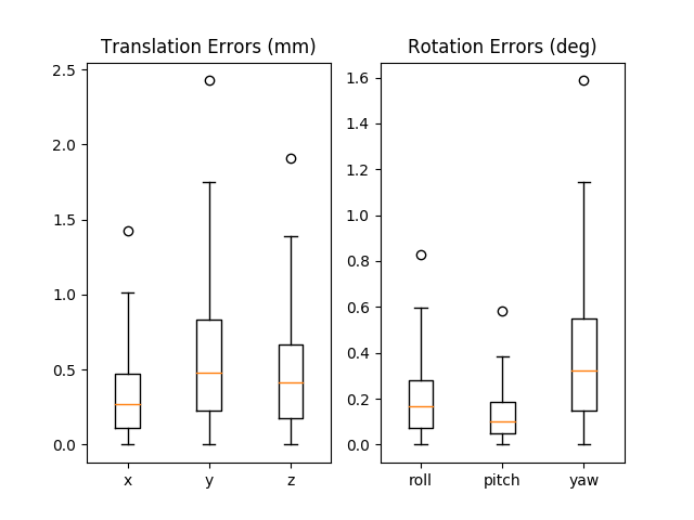
(c) Distributions of translation errors and rotation errors represented by box plots for connector A2. Note that A2 is not involved in the training set.

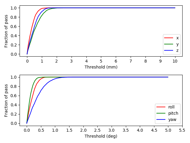
(d) Percentage of pass vs threshold curves for connector A2. Note that A2 is not involved in the training set.

Figure 5: Quantitative experiment results of $M_{8}$ on the test set

TABLE IV: Errors of model $M_{8}$ on the test set

Object	$\mathbf{e_{x}}$/mm	$\mathbf{e_{y}}$/mm	$\mathbf{e_{z}}$/mm	$\mathbf{e_{\phi}}$/°	$\mathbf{e_{\theta}}$/°	$\mathbf{e_{\psi}}$/°
A1	0.17	0.30	0.23	0.12	0.13	0.26
A2	0.36	0.55	0.43	0.21	0.14	0.42
A3	0.23	0.29	0.32	0.13	0.12	0.25
B1	0.19	0.32	0.25	0.14	0.11	0.25
B2	0.22	0.34	0.36	0.15	0.12	0.25
B3	0.18	0.39	0.40	0.13	0.11	0.21
C1	0.20	0.34	0.24	0.14	0.11	0.21
C2	0.16	0.28	0.33	0.11	0.10	0.22
C3	0.20	0.28	0.37	0.11	0.10	0.21

In Figure 5, the model has achieved very high accuracy on the 8 connectors that the network has seen in the training: the translation estimations were around 0.25 mm or better on average, and rotation estimations were around 0.2 degrees or better on average. Except for very few outliers, the vast majority of errors fell below 1.0 mm and 0.8 degree resulting in a steep fraction of pass versus threshold graphs.

The performance on the test set of A2, which was novel to the network, was not as good as that of the other 8 connectors but still highly accurate. The mean errors reached around 0.5 mm and 0.3 degrees. The fraction of pass versus threshold graphs are not as steep but the vast majority of errors still fall below 1.7 mm and 1.2 degrees.

VI-B2 Performance on actual insertion

similar to the experiments conducted with the model $M_{A1}$, we firstly adjusted the pose the robot to obtain $I_{ref}$. We also defined this end-effector pose as the reference pose, $T_{ref}$.

Instead of moving base like in the previous experiment which required human intervention, we automated this experiment by randomly moving the end-effector.

Note that the network can estimate the camera displacement $T_{\Delta}$ from any initial pose A to current pose B, but in order to perform a successful insertion, the reference pose $T_{ref}$ was always used as the pose A.

We then randomly choose a new pose the same way in the Sample Collection and Dataset section, we called it the test pose $T_{test}$. An image $I_{test}$ was captured at the test pose. The network was tasked to estimate a transformation $T_{\Delta}$ to move the pose back to the reference pose.

$T_{est}$ was computed the same way as that in the experiment with $M_{A1}$. If the estimation was perfect, $T_{est}$ should coincide with $T_{ref}$.

The end-effector was then moved to $T_{est}$ followed by descending end-effector to attempt the insertion. For each connector, 25 trials were conducted running on model $M_{8}$.

TABLE V: Performance of model $M_{8}$ on actual insertion

	#Success	#Total Attempts	Percentage(%)
A1	24	25	96
A2	24	25	96
A3	24	25	96
B1	25	25	100
B2	23	25	92
B3	25	25	100
C1	25	25	100
C2	25	25	100
C3	25	25	100
Overall	195	200	97.5

Table V shows that the network was able to achieve extremely high accuracy. Note that the connector A2 (in bold) was not involved in the train set, yet, the network was performing very well on this novel connector after learning similar connectors.

VI-C Iterative estimation for actual insertion with model $M_{A1}$

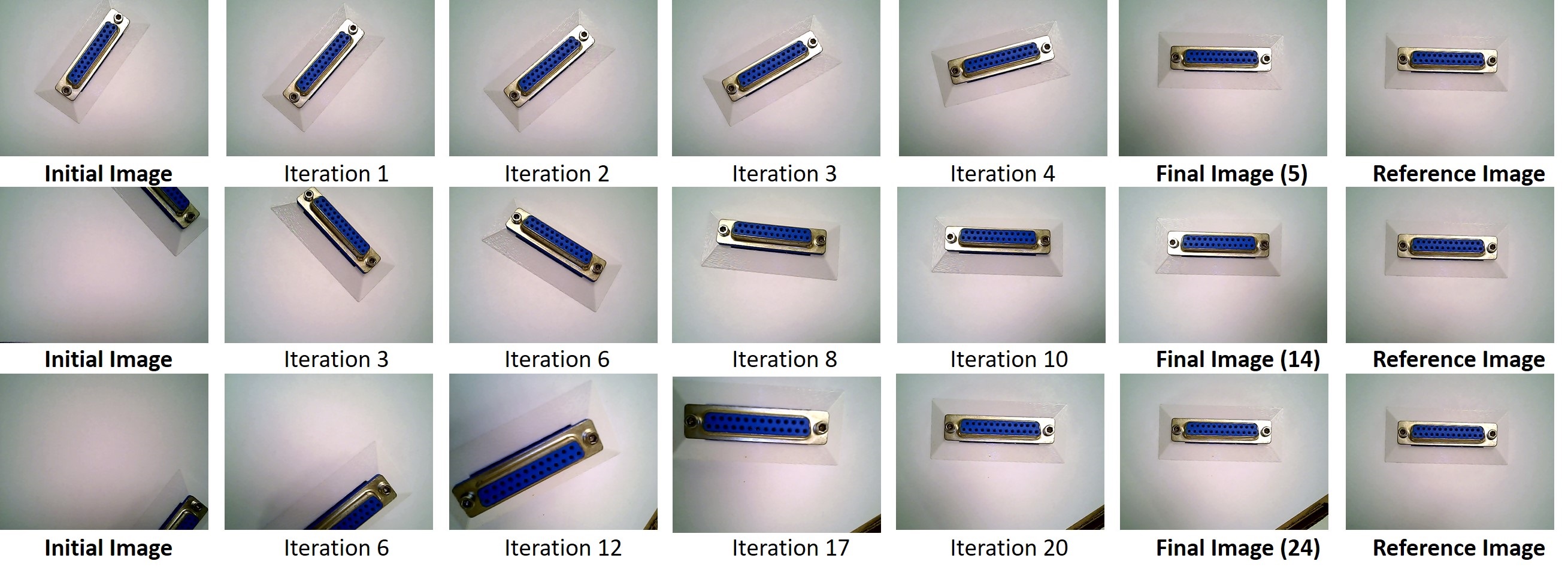
Figure 6: By performing iterative estimations, model $M_{A1}$ was able to guide the robot from extreme starting poses to the reference pose, achieving successful insertions. Selected images from an easy, a medium and a hard test case are shown in the first, the second and the third row respectively (see Table VI for details). Note that model $M_{A1}$ was not trained to estimate pose difference this large. The reference image (in the right-most column) was fixed in the experiment. The number in the bracket of each Final Image caption is the total number of iterations needed to reach the final convergence.

In the insertion experiments reported in Sec VI-A and VI-B, the differences between the initial poses and the reference poses of the robot fell within the sampling range of the train set. Hence, the models’ one-shot estimations were sufficiently precise to achieve successful insertions.

In this third experiment, however, we used model $M_{A1}$ to estimate pose differences that were much larger than the sampling range in the train set. We purposely placed the female connector far away from the image center, such that the pose difference were much larger than transformation labels in the train set. Furthermore, in two of the three test cases, the connectors were even partially occluded in the initial camera images.

Although model $M_{A1}$ could not provide accurate one-shot estimations, it was always able to move the robot closer to the reference pose. Eventually through iterations, the reference pose was always reached in all test cases, allowing successful insertions. The results are tabulated in VI. Camera images at selected iterations are shown in Figure 6.

TABLE VI: Iterative estimation performance. Number of iterations required to converge with various percentage of the female connector visible in the first image. All insertions were successful.

Difficulty	Percentage visible	Test 1	Test 2	Test 3
Easy	100%	5	4	8
Medium	50%	14	17	16
Hard	30%	18	24	15

Moreover, Figure 6 shows that the network is very robust against changing lighting conditions as the final image of the second row has different reflection pattern compared to the reference image. The network is also robust against noises such as blurry image (iteration 17 of the last row was captured when the camera was very close to the connector) and minor changes in the background (iteration 12-24 of the last row, the edge of the A4-sized paper was captured and this was never included in the training set).

VII Conclusion

We present a Siamese convolutional neural network as the last piece to complete the jigsaw of deep learning-based visual servoing. By one-shot estimation, it achieves extremely high accuracy in camera pose estimation (less than 0.6 mm in translation and 0.4 degrees in rotation), which makes it a plausible solution to difficult real-world application such as low-tolerance insertion.

In addition, the network is able to handle large pose difference if used iteratively, even it has only been trained to handle the fine difference. This makes the network a standalone visual servoing solution.

Instead of running evaluations on the test sets, we have demonstrated the model’s exceptional performance (97.5% success rate) on actual insertion task with VGA-connectors. The model is even robust against changing light conditions and able to handle a novel connector through training of a few similar counterparts.

In the future, various scenes can be furthered added to the dataset by replacing the white pixels with other colors to improve generalization across different environments.

References

- [1] S. Hutchinson, G. D. Hager, and P. I. Corke, “A tutorial on visual servo control,” IEEE Transactions on Robotics and Automation, vol. 12, no. 5, pp. 651–670, Oct 1996.
- [2] Q. Bateux, E. Marchand, J. Leitner, F. Chaumette, and P. Corke, “Training deep neural networks for visual servoing,” in 2018 IEEE International Conference on Robotics and Automation (ICRA), May 2018, pp. 1–8.
- [3] A. Saxena, H. Pandya, G. Kumar, A. Gaud, and K. M. Krishna, “Exploring convolutional networks for end-to-end visual servoing,” in 2017 IEEE International Conference on Robotics and Automation (ICRA), May 2017, pp. 3817–3823.
- [4] K. Deguchi, “A direct interpretation of dynamic images with camera and object motions for vision guided robot control,” International Journal of Computer Vision, vol. 37, pp. 7–20, 06 2000.
- [5] J. Bromley, I. Guyon, Y. LeCun, E. Säckinger, and R. Shah, “Signature verification using a ”siamese” time delay neural network,” in Proceedings of the 6th International Conference on Neural Information Processing Systems, ser. NIPS’93. San Francisco, CA, USA: Morgan Kaufmann Publishers Inc., 1993, pp. 737–744.
- [6] D. G. Lowe, “Distinctive image features from scale-invariant keypoints,” Int. J. Comput. Vision, vol. 60, no. 2, pp. 91–110, Nov. 2004. [Online]. Available: https://doi.org/10.1023/B:VISI.0000029664.99615.94
- [7] E. Tola, V. Lepetit, and P. Fua, “Daisy: An efficient dense descriptor applied to wide-baseline stereo,” IEEE Transactions on Pattern Analysis and Machine Intelligence, vol. 32, no. 5, pp. 815–830, May 2010.
- [8] H. Bay, A. Ess, T. Tuytelaars, and L. Van Gool, “Speeded-up robust features (surf),” Comput. Vis. Image Underst., vol. 110, no. 3, pp. 346–359, Jun. 2008. [Online]. Available: http://dx.doi.org/10.1016/j.cviu.2007.09.014
- [9] E. Rublee, V. Rabaud, K. Konolige, and G. Bradski, “Orb: An efficient alternative to sift or surf,” in 2011 International Conference on Computer Vision, Nov 2011, pp. 2564–2571.
- [10] A. Kendall, M. Grimes, and R. Cipolla, “Posenet: A convolutional network for real-time 6-dof camera relocalization,” in 2015 IEEE International Conference on Computer Vision (ICCV), Dec 2015, pp. 2938–2946.
- [11] I. Melekhov, J. Ylioinas, J. Kannala, and E. Rahtu, “Relative camera pose estimation using convolutional neural networks,” in Advanced Concepts for Intelligent Vision Systems - 18th International Conference, ACIVS 2017, Proceedings, ser. Lecture Notes in Computer Science. Germany: Springer Verlag, 2017, pp. 675–687, jufoid=62555.
- [12] L. J. Charco, B. X. Vintimilla, and A. D. Sappa, “Deep learning based camera pose estimation in multi-view environment,” in 14th IEEE International Conference on Signal Image Technology & Internet based Systems (SITIS 2018), Nov 2018.
- [13] H. Aanæs, R. R. Jensen, G. Vogiatzis, E. Tola, and A. B. Dahl, “Large-scale data for multiple-view stereopsis,” International Journal of Computer Vision, pp. 1–16, 2016.
- [14] A. Dosovitskiy, P. Fischer, E. Ilg, P. Häusser, C. Hazirbas, V. Golkov, P. v. d. Smagt, D. Cremers, and T. Brox, “Flownet: Learning optical flow with convolutional networks,” in 2015 IEEE International Conference on Computer Vision (ICCV), Dec 2015, pp. 2758–2766.
- [15] C. Collewet and E. Marchand, “Photometric visual servoing,” IEEE Transactions on Robotics, vol. 27, no. 4, pp. 828–834, Aug 2011.
- [16] P. Agrawal, J. Carreira, and J. Malik, “Learning to see by moving,” in 2015 IEEE International Conference on Computer Vision (ICCV), Dec 2015, pp. 37–45.
- [17] J. Deng, W. Dong, R. Socher, L.-J. Li, K. Li, and L. Fei-Fei, “ImageNet: A Large-Scale Hierarchical Image Database,” in CVPR09, 2009.
- [18] D. Held, S. Thrun, and S. Savarese, “Learning to track at 100 fps with deep regression networks,” in European Conference on Computer Vision (ECCV). Springer, October 2017.
- [19] N. Schneider, F. Piewak, C. Stiller, and U. Franke, “Regnet: Multimodal sensor registration using deep neural networks,” in 2017 IEEE Intelligent Vehicles Symposium (IV), June 2017, pp. 1803–1810.