Generation of ice states through deep reinforcement learning

Abstract

We present a deep reinforcement learning framework where a machine agent is trained to search for a policy to generate a ground state for the square ice model by exploring the physical environment. After training, the agent is capable of proposing a sequence of local moves to achieve the goal. Analysis of the trained policy and the state value function indicates that the ice rule and loop-closing condition are learned without prior knowledge. We test the trained policy as a sampler in the Markov chain Monte Carlo and benchmark against the baseline loop algorithm. This framework can be generalized to other models with topological constraints where generation of constraint-preserving states is difficult.

I Introduction

Ice models Lieb (1967) are the simplest models that can describe the statistical properties of proton arrangement in water ice Pauling (1935), and spin configurations of spin ices Bramwell and Gingras (2001). The ground states in the ice model follow a local constraint, called the ice rule. Due to this constraint, performing local changes in a given ice configuration does not create a new ice state. The loop algorithm, widely used in the Monte Carlo sampling of ice models, generates ice states by exploiting the fact that the difference between two ice configurations are in the form of closed loops Rahman and Stillinger (1972); Yanagawa and Nagle (1979); Barkema and Newman (1998). This is an example where an efficient algorithm generating new constraint-satisfying states emergences from clever inspection of sample states. We want to explore how to automate this type of discovery with machine learning techniques and provide a proof-of-principle implementation.

Efficient state generation is important, in particular, in Markov chain Monte Carlo (MCMC) Landau and Binder (2014); Newman and Barkema (1999). To generate statistically sound samples in the simulation, we need to reduce the autocorrelation between samples in the Markov chain. This can be achieved by clever design of update proposals; for example, in the case of two-dimensional ferromagnetic Ising model, cluster updates such as Swendsen-Wang and Wolf algorithms Swendsen and Wang (1987); Wolff (1989) are powerful methods to reduce the effects of critical slowing down near the critical point and allow for precise extraction of physics with larger systems. However, these cluster algorithms are normally designed for specific models and it is hard to generalize.

Recently, a new class of proposals termed self-learning Monte Carlo, which uses configurations generated by a small size simulation to train an effective model, and draws samples from the effective model to generate new configurations, have demonstrated success in improving of the efficiency of both classical and quantum Monte Carlo simulations Liu et al. (2017a); Nagai et al. (2017); Liu et al. (2017b); Xu et al. (2017). However, the amount of training data required for a successful training normally scales with the complexity of the effective model. Another class of proposals uses the generative models based on deep neural networks in order to generate new samples. The restrict Boltzmann machine, a neural network architecture connected to the the real-space renormalization group Mehta and Schwab (2014), has been used to generate Monte Carlo samples to study thermodynamics Torlai and Melko (2016) and to accelerate Monte Carlo simulations Huang and Wang (2017). The generative adversarial network Goodfellow et al. (2014), where two neural networks contesting with each other, is used to generate configurations for two-dimensional Ising model Liu et al. (2017) and for a complex scalar field in two dimensions with a finite chemical potential Zhou et al. (2018). The success behind these methods relies on the fact that the underlying distribution of the configurations is continuous in the thermodynamic limit; that is, all configurations generated by the neural networks are allowed. On the other hand, direct application of these methods to generate configurations for the topologically constrained model can be difficult. Here not all configurations generated by the neural network can satisfy the constraint. Therefore, a new scheme is highly coveted.

In this paper, we explore how to apply a reinforcement learning framework Sutton and Barto (2018) to generate new configurations that satisfy the ice rule constraint. Reinforcement learning has demonstrated remarkable abilities in achieving better than human performances on video games Mnih et al. (2015), and the game of Go Silver et al. (2016, 2017). Recently it has also been applied to quantum physics research such as quantum control Fösel et al. (2018), quantum error correction Sweke et al. (2018); Liu and Poulin (2018); Poulsen Nautrup et al. (2018), quantum experiment design Melnikov et al. (2018). In a reinforcement learning setup, a machine agent interacts with its environment. At each time step, the agent takes an action on the current state of the environment, and then receives a calculated reward from the observation of the consequence of this action. A feasible reinforcement learning algorithm seeks to maximize the total reward through a trial-and-error learning procedure. We will utilize this feature to design an algorithm to adaptively search for a move from an ice state to another.Similar ideas have been explored recently by the policy-guided Monte Carlo (PGMC) proposal Bojesen (2018) to improve MCMC sampling. The policies in Ref. Bojesen (2018) are modeled with simple functions and the best policy is obtained by optimizing parameters in these models. Here we instead model the policy as a deep neural network, and build the physical constraints into the design of the reward function. Therefore, we can take advantage of the recent progress in the reinforcement learning research to train an agent with a simple set of actions to explore the physical environment. The best policy naturally emerges out of the agent’s interaction with the environment, subjected to the reward design. This scheme should serve as a general framework to search for methods to generate topologically constrained states in other physical models.

The rest of the paper is organized as follows: In Sec. II, we introduce the square ice model and the conventional loop algorithm. In Secs. III and IV, we introduce the deep reinforcement learning framework we use. In Sec. V, the training process and agent behavior will be discussed. We use the trained policies as samplers for Markov chain Monte Carlo in Sec. VI. Finally, we conclude in Sec. VII.

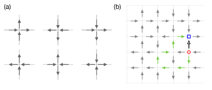
Figure 1: (Color online) (a) Local spin configurations that satisfy the 2-in-2-out ice rule at each vertex. (b) Flipping a spin (unfilled arrow) in an ice state creates a pair of defects, resulting in a high-energy state. Propagation of a single defect (red circle) by flipping green (bright) spins creates no additional defects. When the loop is closed, the pair of defects (red circle and blue square) annihilates and a new ice configuration is generated.

II Square Ice Model

Here we consider a two-dimensional ice model on a square lattice Lieb (1967). At each vertex, the arrangement of spins satisfies the ice rule: two spins pointing into and two pointing out of the vertex (Fig. 1(a)). There exist six types of vertices that satisfy this constraint and all other types of vertices are considered defects with higher energy. This is the reason why ice models are sometimes referred as six-vertex models Lieb (1967); Baxter (2016). Ice states, therefore, correspond to spin configurations with zero defects. All ice states have the same energy, and they form an extensively degenerate ground state manifold with a finite residual entropy at zero temperature of $S/N=k_{B}\ln W$ where $W=\left(4/3\right)^{3/2}$ Lieb (1967). They are, however, sparsely populated in the configuration space of all possible spin configurations (Fig. 2). Consider, for example, flipping a random spin from a given ice configuration, and the two neighboring vertices connected by this spin violates the ice rule constraint, creating a pair of topological defects of three-in-one-out and one-in-three-out vertices (Fig. 1(b)) . The configurations that satisfy the ice rules are thus separated by large energy barriers and the conventional Metropolis single-spin flip update scheme will fail. However, it is possible to flip a series of neighboring spins to bring one ice configuration to another. By examining the difference between two ice states, it is clear that they differ only by spins forming closed-loops. This indicates loop-like updates can bypass the energy barrier and reach a new ice configuration.

The simplest algorithm to generate random closed loops is the long loop algorithm Rahman and Stillinger (1972); Yanagawa and Nagle (1979). In each round of the algorithm, one vertex is chosen as a starting point. One of the two out-going spins from this vertex is chosen with equal probability Barkema and Newman (1998). Following this spin to the connecting vertex and choose one of the two out-going spins with equal probability. Repeat the process until the starting vertex is reached and the loop closes. All the spins on the resulting loop are reversed to update the configuration while preserving the ice rule. Since at each vertex out-going spins are chosen with equal probability, there are $2^{m}$ possible paths for a given starting point, where $m$ is the size of the loop. This algorithm gives an example of how one can generate a new ice configuration by going through a series of highly unfavorable configurations in order to achieve the final goal. This philosophy is indeed very similar to that of the reinforcement learning that the best long-term strategy may involve short-term sacrifices. It is natural to explore the reinforcement learning scheme to generate new ice configurations.

Figure 2: (Color online) Ice configurations are sparsely populated in the full configuration space. Each red dot represents an ice configuration. The distance between the red dots measures the difference between ice configurations. The black (dashed) circle indicates the configurations reachable by a single-spin flip. The probability $P$ for each ice configuration is a $\delta$-function; therefore a single-spin flip alone can not reach another ice configuration. By constructing a path (curved arrows) of single-spin flip moves, it is possible to reach a new ice configuration.

III Reinforcement Learning

Reinforcement learning (RL) is the branch of machine learning concerned with making sequence of decisions for long-term profit  Sutton and Barto (2018). The central idea of RL is to consider a machine agent situated in an environment. At each time step, the agent takes an action on the current state of the environment, and then receives a calculated reward from the observation to the outcome of this action. A feasible RL algorithm seeks to maximize the total reward for the agent from an unknown environment through a trial-and-error learning procedure. We model the agent policy $\pi_{\theta}$ with parameters $\theta$ using deep and convolutional neural networks.

The core idea of our work is to parameterize the proposal operator as the agent policy and search for efficient transitions in the configuration space under given physical constraints. In order to automate the search process, we extend the original Markov chain to a Markov decision process (MDP), by indicating how a state $s_{t}$ transitions into a new state $s_{t+1}$ using the action $a_{t}$ with the transition probability $p(s_{t+1}|s_{t},a_{t})$. The parametrized policy $\pi_{\theta}(a|s)$ specifies the probability of the action $a$ the agent will take given the state $s$. A reward function $r_{t}\equiv r(s_{t},a_{t})$ is associated with each state-action pair $\{s_{t},a_{t}\}$. A move in the Markov chain can, therefore, be decomposed into a series of decision-makings in the MDP (Fig. 3),

$$p(s_{0}\to s_{T})=p(s_{0})\prod_{t=0}^{T-1}\sum_{a_{t}}\pi_{\theta}(a_{t}|s_{t})p(s_{t+1}|s_{t},a_{t})$$ (1)

The policy $\pi_{\theta}$ can be regarded as a proposal operator in the conventional MCMC.

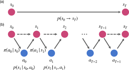
Figure 3: (Color online) A global move in the Markov chain (a) from state $s_{0}$ to $s_{T}$ can be decomposed into a sequence of local moves. By extending the Markov chain to a Markov decision process, the policy $\pi(a|s)$ serves as a transition operator, making local decisions, to generate a global movement in state space.

We briefly sketch the policy gradient scheme used in this work and refer the interested readers to Refs. Sutton and Barto (2018); Neftci and Averbeck (2019) for details.

Given a trajectory of the state-action pairs $\tau=(\{s_{0},a_{0}\},\{s_{2},a_{2}\},\ldots)$ in the MDP, the goal of RL is to maximize the expected future return, i.e., the weighted sum of rewards. The objective function can be defined as a function of the policy,

$$J(\pi_{\theta})=\mathbb{E}_{\pi}[R(\tau)]=\sum_{\tau}\pi_{\theta}(\tau)R(\tau),$$ (2)

where $\mathbb{E}_{\pi}$ denotes the expectation value is evaluated along a trajectory $\tau$ following the policy $\pi$. The total expected return along the trajectory $\tau$ is given as $R(\tau)=\sum_{t=0}^{T-1}\gamma^{t}r_{t}$, where $0\leq\gamma<1$ denotes a discounting factor. The general method for estimating the gradients of an expectation function is using the score function estimator Shapiro (2003), and the model-free policy gradient can be obtained as

$$\nabla_{\theta}J(\pi_{\theta})=\mathbb{E}_{\pi}[\nabla_{\theta}\log\pi_{\theta}(\tau)R(\tau)].$$ (3)

The optimal parameter $\theta$ can be obtained by the gradient ascent $\theta\leftarrow\theta+\alpha\nabla J(\pi_{\theta})$ with the learning rate $\alpha$.

To estimate how good it is for the agent to be in state $s$, following policy $\pi$, we define a state-value function,

$$V^{\pi}(s)=\mathbb{E}_{\pi}\left[\left.\sum_{k=0}\gamma^{k}r_{t+k+1}\right|s_{t}=s\right],$$ (4)

which estimates the expected future rewards starting from state $s$. To estimate $V^{\pi}$, one starts from a random initial state and follow $\pi(a|s)$ to generate a trajectory to accumulate average return achieved from each state. Given enough samples, the average should converge to the optimal $V_{\pi}$. The value function allows us to compare the policies: a policy $\pi$ is better than or equal to a policy $\pi^{\prime}$ if only if $V_{\pi}(s)\geq V_{\pi^{\prime}}(s)$ for all $s$ Sutton and Barto (2018).

We use the Asynchronous Advantage Actor-Critic (A3C) algorithm Mnih et al. (2016) to perform the training. The value function $V^{\pi}_{\phi}(s)$ is also parametrized by a neural network with parameter $\phi$, and the policy gradient is given by

$$\nabla_{\theta}J(\pi_{\theta})=\mathbb{E}_{\theta}\left[\sum_{t}\nabla_{\theta}\log\pi_{\theta}(a_{t}|s_{t})A^{\pi}_{\phi}(s_{t},a_{t})\right],$$ (5)

where $A^{\pi}_{\phi}(s_{t},a_{t})=r_{t}+\gamma V^{\pi}_{\phi}(s_{t+1})-V^{\pi}_{\phi}(s_{t})$ is an estimate of the advantage function Mnih et al. (2016). The parameterized value function $V^{\pi}_{\phi}(s)$ is trained to predict the expected future return that reduces the variance of policy gradient and stabilizes the training process. In practice, the training is done using the loss function,

$$L(\theta,\phi)=-\left[\sum_{t}\Big{(}\log\pi_{\theta}(a_{t},s_{t})A^{\pi}_{\phi}(t)-||V^{\pi}_{\phi}(s_{t})-R_{t}||^{2}\Big{)}+\lambda\pi_{\theta}(a_{t}|s_{t})\log\pi_{\theta}(a_{t}|s_{t})\right].$$ (6)

The first term describes the policy loss, the second term gives the estimation of the value function, and the last term provides the entropy regularization. In our experience that the policy entropy term not only promotes exploration but provides a sensible indicator in the training process. The asynchronous algorithm launches several independent agents sampling trajectories from distinct environments. A central network holds shared parameters and is updated asynchronously by many agents. In other words, each agent explores the state space simultaneously from different initial states. This approach prevents the machine from overfitting to some specific configuration and generalizes the policy search. Eight independent agents are used in our program to update eight independent ice states simultaneously.

IV Agent-Environment Interface

We implement an interactive interface for the interaction between the machine agent and the physical environment compatible with OpenAI Gym Brockman et al. (2016). Two kinds of observations of the environment are provided to the agent. The global observation $O_{\rm global}$ monitors the configuration changes $C_{t}=s_{t}-s_{0}$ between the initial ice state $s_{0}$ and the current state $s_{t}$. The local observation $O_{\rm local}$ monitors local information such as the neighboring spins $\sigma_{i}$, the fraction of configuration change $\Delta C$ defined as the ratio of the number of flipped spins and the total number of spins. A state in the MDP is a composite of local and global observations, $s=[O_{\rm local},O_{\rm global}]$.

In deep reinforcement learning, the policy and value functions are both approximated by neural networks. In practice, the value function usually shares weights with the policy approximator Vinyals et al. (2017); therefore, the same network is used for making action decision and predicting the future return. We model the agent with two types of networks: (a) Local network, where only local observation is used as input information; (b) Multi-channel network, where local and global observations are combined. Figure 4 shows the architecture of the multi-channel neural networks for the agent Vinyals et al. (2017). The local information is fed into two layers of feedforward networks while the global observation is extracted through two layers of convolutional neural networks before they are concatenated. The specification of the neural network architecture and hyperparameters for training can be found in App. B. In the following, we call the policy obtained from the local network as NN policy, and multi-channel network as CNN policy.

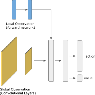
Figure 4: (Color online) Architecture of the multi-channel neural network for the agent. For the NN policy, global observation is turned off.

The actions that the agent located at spin $\sigma$ can execute on the environment contains two types of operations: Select and flip a neighboring spin $\sigma_{i},i\in\{0,..,5\}$, $a_{i}$, and propose an update, $a_{\text{update}}$ (Fig. 6). At each step, the agent is located at a spin and execute one action from the action space according to the policy $\pi_{\theta}(a|s)=[p(a_{0}),\ldots,p(a_{5}),p(a_{\textrm{update}})]$, the probability distribution of taking an action $a$ for a given state $s$. We note that all six neighbors are available in our RL framework, while in the conventional loop algorithm only two are allowed. For example, the policy for the loop algorithm corresponding to the local environment shown in Fig. 6 is $\pi_{\text{loop}}=[0,0,0,0,1/2,1/2,0]$ since only the two outward pointing spins can be chosen with equal probability. Therefore, we design the actions in a less restrictive way and allow the agent to learn the effective trajectory by exploring the physical model. In addition, the action $a_{\text{update}}$ provides flexibility for the agent to terminate at any step. As we will show in the following, after sufficient exploration of the physical environment, the agent tends to perform $a_{\text{update}}$ only when a loop is formed.

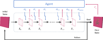
Figure 5: (Color online) Architecture of agent-environment interface. From an initial ice state, the agent keeps executing actions on the environment and receiving corresponding rewards until the agent decides to make an update and finishes the episode. In the final configuration, only the spins altered by the agent are depicted.

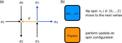
Figure 6: (Color online) (a) Local environment for an agent located at spin $\sigma$. There are six neighboring spins that the agent can choose to flip next. The blue spins $\sigma_{4}$ and $\sigma_{5}$ correspond to the possible choices in the loop algorithm. (b) Two types of actions that the agent can take: Flipping a neighboring spin or applying an update to the spin configuration.

The objective of RL is maximizing the cumulative rewards. In playing Atari games, the game score is an obvious choice for reward. In our application, however, searching for update patterns hidden in the environment does not translate directly into an optimization problem. Therefore, the reward function serves as the guiding principal to inform the agent whether a new ice state is generated. The restricted environment itself would be the main reason that versatile policies emerge during the training process Heess et al. (2017). We design the sparse reward function as a step function given at the end of each episode,

$$r_{T}(s,a)=\left\{\begin{array}[]{ll}r_{g}=1\text{, if the final state is an ice state}\\ r_{f}=0\text{, otherwise}\\ \end{array}\right.$$

Once the action $a_{\text{update}}$ is executed, the episode will be terminated and the agent will receive the reward $r_{T}$. This encourages the agent to perform $a_{\text{update}}$ only when the environment is in a defect-vacuum state and thus generate a closed loop in each episode. Since the closed-loop condition is relatively rare, at most of the steps the agent receives no reward signals. This kind of approximately silent environment usually causes inefficient sampling and vanishing gradient in the training process. To avoid this problem, we also define a stepwise reward $r_{s}(s,a)$ to encourage the agent to explore the environment and attempt to generate larger loops. The stepwise rewards are assigned at each step regardless of the action taken by the agent and chosen to be relative small such that the agent recognizes $r_{g}$ as the ultimate goal Ng et al. (1999). In practice, we keep the ratio of the stepwise reward to the goal reward as $r_{s}/r_{g}\sim\mathcal{O}(N^{-1})$, where $N$ is the number of sites of the system.

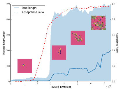
Figure 7: (Color online) Agent training process for $L=16$. The shaded area presents the loop length distribution, bounded by maximum and minimum lengths. The dashed line represents the acceptance ratio of the agent’s proposed move. At the early stage of learning, the agent only creates $2\times 2$ smallest loops to obtain the goal rewards. In this phase, agent learns appropriate timing to execute $a_{\text{update}}$. Based on the learned small-loop strategy, the agent realizes that ice rule allows for larger loops to occur if there are no more defects are generated in the process. After $7\times 10^{5}$ training steps, the acceptance ratio of the agent-proposed moves reaches close to 100%.

V Training Process and Agent Behavior

At the beginning of the training process, the agent lacks any prior knowledge about the physical environment and performs random moves to collect data. After a few trials, the agent quickly gains the ability to generate a $2\times 2$ square loop, the smallest closed loop providing a non-zero goal reward. In the absence of stepwise reward, the agent would exploit this policy by proposing square loops frequently. However, the stepwise reward encourages the agent to explore the possibilities beyond the square loop. The distribution of loop length as a function of training time is shown in Fig. 7. After about $3\times 10^{5}$ training episodes, the agent becomes proficient at performing larger random loops and executes the update action correctly. While the maximum loop length shows a clear jump at this point, the average loop size grows steadily. The acceptance ratio of the proposed moves also grows steadily during training, and approaches 100% at later stage of the training.

In order to generate a new ice configuration, the agent needs to learn to annihilate the pair of defects by closing the loop. The well-trained agent can be regarded as a policy-guided machine in which the policy $\pi(a|s)$ does the decision-making of local spin flipping and the state-value function $V(s)$ serves as the loop-closing detector. In Fig. 8, we present the decision-making process by the agent near the end of one episode. In most of the steps, the policy distribution shows two possible candidate spins with almost equal probability. This behavior is similar to that of the conventional loop algorithm where one of the two out-going spins are selected with equal probabilities Barkema and Newman (1998). However, there exist time steps that the agent takes deterministic action to move in certain direction. This indicates the agent is exploiting knowledge acquired during the training. Once the loop is closed, the agent decides to perform an update action ($a_{\text{update}}$) and terminate the episode with certainty. This behavior is consistent with the loop closing condition in the loop algorithm. We can also use the state-value function $V(s)$ as an indicator of the agent behavior since it implies the cumulative future reward. In Fig. 9 we show the evolution of $V(s)$ in the process of a single loop formation. When the episode starts, the system is close to an ice state and the value function gives high expectation value. After a few steps of executing the local policy, the value function drops to a local minimum as ends of the segment move apart and going toward the opposite directions (inset A in Fig. 9). During the exploration stage, it is possible that two ends move closer, and the value function reaches a local maximum (inset B in Fig. 9). At the final step, the value function jumps suddenly, anticipating the goal reward to be obtained by performing the update action (inset C in Fig. 9). This indicates that the state-value function plays the role of loop-closing detector and recognizes the global pattern of the environment.

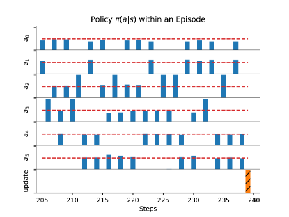
Figure 8: (Color online) Decision-making process of the agent illustrated by the policy $\pi(a|s)$. Most of the time, the agent behaves in a similar way to conventional long-loop algorithm which makes stochastic selection from two outgoing spins (with probability $0.5$, denoted by red dashed lines). When the trajectory forms a closed loop, the agent executes the update operation with full confidence (orange striped bar).

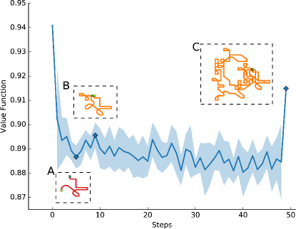
Figure 9: (Color online) State-value function $V^{\pi}(s)$ shows the expected future reward in the process of a loop formation. Shaded area shows the distribution of the value, bounded by the maximum and minimum value. A local minimum occurs when endpoints (circle and square) are far apart (A), and a local maximum occurs when two endpoints move closer to each other (B). When a closed loop emerges, the value function shows a jump and large reward is expected (C).

VI Sampling using trained policies

As mention in Sec. IV, two types of policies are trained by supplying different sets of observations to the agent. The NN policy is trained with only the local observation $O_{\textrm{local}}$, and the CNN policy is trained with both the local and global observations $O_{\textrm{local}}$ and $O_{\textrm{global}}$. We will use these trained policies as samplers in the MCMC for the square ice model. With the capacity of deep learning models, it is possible the network simply memorizes the configurations it generated in the learning process. In order to check this, we start the trained agents from the same ice configuration at the same initial position to perform one update. We expect that the agent’s behavior should become independent of the initial starting position and explore the space without special preferences. The baseline loop algorithm shows the probability of each site being visited rapidly smears out (Fig. 10(a)) with the number of steps. We observe, on the other hand, strong memory effects in the NN policy (Fig. 10(b)) such that the agent tends to linger around the initial site; while the CNN policy behaves similar to the baseline loop algorithm (Fig. 10(c)).

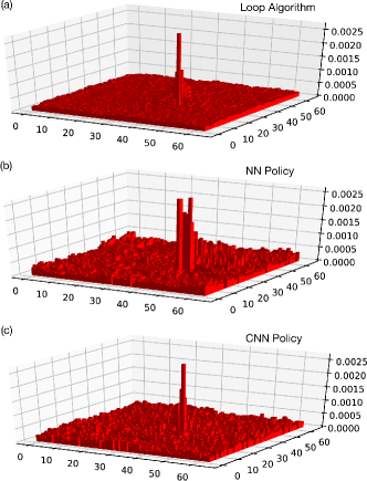
Figure 10: (Color online) Probability that a site is visited starting from the same initial site and ice configuration for (a) loop algorithm, (b) NN policy, and (c) CNN policy. The NN policy shows significant memory effects while the CNN policy shows similar behavior as the loop algorithm.

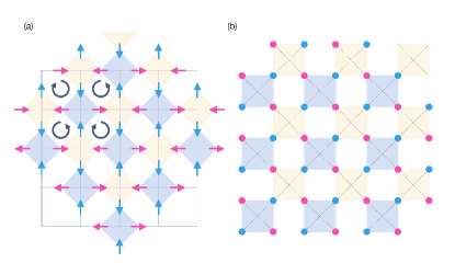
Figure 11: (Color online) Equivalence mapping between the (a) vertex spins on a square lattice and (b) Ising variables on a checkerboard lattice by a 45^∘ rotation. This specific configuration corresponds to the ice state with a Néel order, where a regular vortex pattern (black circular arrows) is shown.

We now use the trained policies to propose samples in the Markov chain Monte Carlo to compute physical observables. In particular, we are interested in correlation functions such as the magnetic structure factor defined as

$$S(\mathbf{q}) =\frac{1}{L^{2}}\left\langle s_{\mathbf{q}}s_{-\mathbf{q}}\right\rangle,\mbox{where }s_{\mathbf{q}}=\sum_{r}s_{\mathbf{r}}e^{-i\mathbf{q}\cdot\mathbf{r}},$$ (7)

where the Ising variables $s_{\mathbf{r}}$ on a checkerboard lattice are obtained by an equivalence mapping from the vertex spins on a square lattice (Fig. 11), and $\mathbf{q}$ is the momentum. In order to reproduce the correct correlation, the configurations should be sampled according to the underlying distribution. All ice configurations in the square ice model are equally probable; that is, all ice configurations should be sampled equally for the sampling to be ergodic. Again, we use the structure factor generated by the loop algorithm as our baseline. Fig. 12 shows the spin structure factors using samples generated by different algorithms. Both the NN (Fig. 12(b)) and CNN policies (Fig. 12(c)) can capture the diffuse scattering present in the model; however, it is clear that correlation is biased for the trained policies. We plot in Fig. 12(d) the structure factor $S(\mathbf{q})$ along the high symmetry direction in the first Brillouin zone. We find that some weight of the diffusing scattering is missing in the trained policies, and spectral weight is shifted toward the $\mathbf{Q}=(\pi/2,\pi/2)$ point, indicating bias toward the Néel ordered states for the trained policies. Surprisingly the CNN policy is biased more toward the Néel states than the NN policy, although the former has less memory effects due to the global view. In the Néel order, spins arrange in a regular vortex pattern (Fig. 11). This pattern requires a global view to establish; thus, the CNN policy tends to bias more toward the Néel states.

Clearly, the trained policies are not sampling all the ice states equally, and the ergodicity is broken. This is related to the fact that the machine policy contains actions that makes deterministic moves. These actions indicate that agent somehow memorizes special spin configurations during the training process. Therefore, directly using the policies as samplers introduces bias in the sampling. This is the consequence of not enforcing the detailed balance condition during the training, but may be corrected if one obtains an estimate of the density of the bias in the transition probability. We note this should not be considered a failure of the current framework since the probability distribution of ice states is multimodal with equal weights, which posts a significant challenge to properly sample. On the other hand, by adjusting the stepwise reward, it is possible to bias the agent to create larger loops. Therefore, this can be used to as an overrelaxation step to decorrelate samples in the Markov chain, when combined with the conventional loop algorithm.

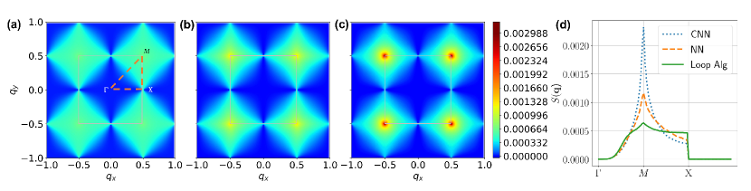
Figure 12: (Color online) The structure factor for $L=64$ computed using the configurations generated from (a) the conventional loop algorithm, (b) the NN policy, and (c) the CNN policy. The gray square indicates the magnetic first Brillouin zone. The NN and CNN policies are trained in a $L=32$ setting and a moving horizon embedding described in the Appendix A is used to generate states for $L=64$. (d) Line cuts of $S(\mathbf{q})$ along high symmetry directions in the first Brillouin zone as indicated in the orange (dashed) lines in (a). Both the trained policies show bias toward the Néel order.

VII Conclusion

In this work, we develop a framework using deep reinforcement learning to generate topologically constrained ice states. We successfully train an agent to propose stepwise actions that when combined together can transit from one ice state to another. By rewarding the agent when a correct ice state is generated, several physical insights emerge out of the training. Although the ice rule is not given explicitly, the agent learns to move in a path without creating additional defects. The agent also learns to distinguish open and closed loops, and perform the update action when the loop closes. The physical constraints are built into the reward function, not the policy itself. By using deep reinforcement learning, we show that the machine can actually learn the global loop pattern and propose updates without prior knowledge of the ice rule. Therefore, it is possible to extend this framework to other physical models. For example, quantum Monte Carlo simulations of quantum spin ice models Henry and Roscilde (2014); Wu et al. (2019); Wang et al. (2018), toric code and related gauge models Trebst et al. (2007); Tupitsyn et al. (2010); Kamiya et al. (2015) have been difficult due to the physical constraints present in the model. The generality of the RL framework presented here can explore an enlarged state space and potentially discover new sampling schemes through the automatic exploration of the machine agent on a constrained model. These update proposals can be used as candidate policies in the PGMC Bojesen (2018) where detailed balance can be satisfied. It would also be interesting to model the policy using neural networks with normalizing flows Dinh et al. (2014); Jimenez Rezende and Mohamed (2015); Dinh et al. (2016); Papamakarios et al. (2017); Li and Wang (2018). Combining the exploration capability of RL with the unbiased control of the training and inference of the reversible policy model can potentially lead to the discovery of efficient MCMC algorithms without detailed balance Suwa and Todo (2010) for constrained models. Finally, we note that the training of the model takes roughly three days on a Xeon workstation, and each inference step of the CNN policy takes about $0.75$ ms. Both the conventional loop algorithm and the CNN policy take about five minutes to generate 1000 loops on a $L=32$ system.

VIII Acknowledgments

Y.-J.K. thanks T. Bojesen for useful discussion and critical reading of the manuscript. This work was supported in part by the Ministry of Science and Technology (MOST) of Taiwan under Grants No. 105-2112-M-002-023-MY3, and 107-2112-M-002 -016 -MY3 , 108-2918-I-002 -032, and by the National Science Foundation under Grant No. NSF PHY-1748958. We are also grateful to the National Center for High-performance Computing for computer time and facilities.

Appendix A Sliding horizon scheme

We train the agent policy in a $L_{t}\times L_{t}$ square lattice with the periodic boundary condition. In general, the trained network can only process fixed input dimension assigned before training. In order to use the agent in a larger system, we exploit the translational invariance of the policy and use the sliding horizon embedding that dynamically crops the input image and moves the horizon together with the agent. The observation information within the $L_{t}\times L_{t}$ window is provided to the agent. When the agent reaches the boundary of the window, the window is recentered around the agent as the agent traversing the $L\times L$ lattice. This scheme provides the agent the view similar to the training stage. It also allows us to access system sizes larger than the training size as presented in the main text.

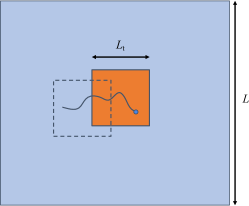
Figure 13: (Color online) The sliding horizon embedding scheme. The trained agent (blue circle) takes input from an $L_{t}\times L_{t}$ window (dark inner square) embedded in a $L\times L$ lattice. Dashed square corresponds to the initial position of the observation window.

Appendix B Network architecture and hyperparameters

Here we present details of the specifications of the neural network architecture and the hyperparameters used in this paper. Table 1 lists the specification of the local and multi-channel networks for the agent. Table 2 lists all of hyperparameters, system settings and environment configurations for future experiment reproductions.

Table 1: Neural network architectures for the agent.

Name	Layer	Size
Local Network, NN Policy	linear (relu)	$32$
	linear (relu)	$64$
	linear (relu)	$128$
	parallel (relu)	$7$, $1$
Multi-channel Network, CNN Policy	linear (relu)	$32$
	linear (relu)	$64$
	conv (relu)	$32,3\times 3$, stride $2$
	conv (relu)	$16,3\times 3$, stride $2$
	concat	$1088$
	linear (relu)	$128$
	parallel (relu)	$7$, $1$

Table 2: Hyperparameters used in training.

Type	Hyperparameter	Value
Training	Solver type	ADAM
	Learning rate	$10^{-4}$
	$\beta_{1},\beta_{2}$ (hparam for ADAM)	$0.9,0.999$ (default)
	Total steps	$10^{9}$
	Update steps	$120$
	Entropy regularization, $\lambda$	$0.0001$
	Exploration	$\epsilon-$greedy, $1\%$
	Gradient clip	$40.0$
	Discount factor $\gamma$	$0.99$
System	Number of parameter server	1 (host)
	Number of workers	8
	Number of policy monitor	1
	TensorBoard process	1
	Evaluation duration	60 seconds
Environment	Lattice size	$L=16$
	Observation shape	$O_{g}:32\times 32\times 1$, $O_{l}:10$
	Action shape	$7$
	Stepwise reward	$+0.001$
	Target reward	$+1.0$
	Timeout steps	$1024$

References

- Lieb (1967) Elliott H. Lieb, “Residual entropy of square ice,” Phys. Rev. 162, 162–172 (1967).
- Pauling (1935) Linus Pauling, “The structure and entropy of ice and of other crystals with some randomness of atomic arrangement,” Journal of the American Chemical Society 57, 2680–2684 (1935), https://doi.org/10.1021/ja01315a102 .
- Bramwell and Gingras (2001) Steven T. Bramwell and Michel J. P. Gingras, “Spin ice state in frustrated magnetic pyrochlore materials,” Science 294, 1495–1501 (2001).
- Rahman and Stillinger (1972) Aneesur Rahman and Frank H. Stillinger, “Proton Distribution in Ice and the Kirkwood Correlation Factor,” The Journal of Chemical Physics 57, 4009–4017 (1972).
- Yanagawa and Nagle (1979) A. Yanagawa and J.F. Nagle, “Calculations of correlation functions for two-dimensional square ice,” Chemical Physics 43, 329 – 339 (1979).
- Barkema and Newman (1998) G T Barkema and M E J Newman, “Monte Carlo simulation of ice models,” Phys. Rev. E 57, 1155–1166 (1998).
- Landau and Binder (2014) David P. Landau and Kurt Binder, A guide to Monte Carlo simulations in statistical physics (Cambridge university press, 2014).
- Newman and Barkema (1999) M. E. J. Newman and G. T. Barkema, Monte Carlo Methods in Statistical Physics (Oxford University Press: New York, USA, 1999).
- Swendsen and Wang (1987) Robert H Swendsen and Jian-Sheng Wang, “Nonuniversal critical dynamics in monte carlo simulations,” Phys. Rev. Lett. Review Letters 58, 86 (1987).
- Wolff (1989) Ulli Wolff, “Collective Monte Carlo updating for spin systems,” Physical Review Letters 62, 361 (1989).
- Liu et al. (2017a) Junwei Liu, Yang Qi, Zi Yang Meng, and Liang Fu, “Self-learning Monte Carlo method,” Physical Review B 95, 041101 (2017a).
- Nagai et al. (2017) Yuki Nagai, Huitao Shen, Yang Qi, Junwei Liu, and Liang Fu, “Self-learning Monte Carlo method: Continuous-time algorithm,” Physical Review B 96, 161102 (2017).
- Liu et al. (2017b) Junwei Liu, Huitao Shen, Yang Qi, Zi Yang Meng, and Liang Fu, “Self-learning Monte Carlo method and cumulative update in fermion systems,” Physical Review B 95, 241104 (2017b).
- Xu et al. (2017) Xiao Yan Xu, Yang Qi, Junwei Liu, and Liang Fu, “Self-learning quantum Monte Carlo method in interacting fermion systems,” Phys. Rev. B 96, 041119 (2017).
- Mehta and Schwab (2014) P. Mehta and D. J. Schwab, “An exact mapping between the Variational Renormalization Group and Deep Learning,” ArXiv e-prints (2014), arXiv:1410.3831 [stat.ML] .
- Torlai and Melko (2016) Giacomo Torlai and Roger G. Melko, “Learning thermodynamics with Boltzmann machines,” Phys. Rev. B 94, 165134 (2016).
- Huang and Wang (2017) Li Huang and Lei Wang, “Accelerated Monte Carlo simulations with restricted Boltzmann machines,” Phys. Rev. B 95, 035105 (2017).
- Goodfellow et al. (2014) I. J. Goodfellow, J. Pouget-Abadie, M. Mirza, B. Xu, D. Warde-Farley, S. Ozair, A. Courville, and Y. Bengio, “Generative Adversarial Networks,” ArXiv e-prints (2014), arXiv:1406.2661 [stat.ML] .
- Liu et al. (2017) Zhaocheng Liu, Sean P. Rodrigues, and Wenshan Cai, “Simulating the Ising Model with a Deep Convolutional Generative Adversarial Network,” arXiv e-prints , arXiv:1710.04987 (2017), arXiv:1710.04987 [cond-mat.dis-nn] .
- Zhou et al. (2018) Kai Zhou, Gergely Endródi, and Long-Gang Pang, “Regressive and generative neural networks for scalar field theory,” arXiv e-prints , arXiv:1810.12879 (2018), arXiv:1810.12879 [hep-lat] .
- Sutton and Barto (2018) R.S. Sutton and A.G. Barto, Reinforcement Learning: An Introduction, Adaptive Computation and Machine Learning series (MIT Press, 2018).
- Mnih et al. (2015) Volodymyr Mnih, Koray Kavukcuoglu, David Silver, Andrei A Rusu, Joel Veness, Marc G Bellemare, Alex Graves, Martin Riedmiller, Andreas K Fidjeland, Georg Ostrovski, et al., “Human-level control through deep reinforcement learning,” Nature 518, 529 (2015).
- Silver et al. (2016) David Silver, Aja Huang, Chris J Maddison, Arthur Guez, Laurent Sifre, George Van Den Driessche, Julian Schrittwieser, Ioannis Antonoglou, Veda Panneershelvam, Marc Lanctot, et al., “Mastering the game of Go with deep neural networks and tree search,” Nature 529, 484–489 (2016).
- Silver et al. (2017) David Silver, Julian Schrittwieser, Karen Simonyan, Ioannis Antonoglou, Aja Huang, Arthur Guez, Thomas Hubert, Lucas Baker, Matthew Lai, Adrian Bolton, et al., “Mastering the game of Go without human knowledge,” Nature 550, 354 (2017).
- Fösel et al. (2018) Thomas Fösel, Petru Tighineanu, Talitha Weiss, and Florian Marquardt, “Reinforcement learning with neural networks for quantum feedback,” Phys. Rev. X 8, 031084 (2018).
- Sweke et al. (2018) Ryan Sweke, Markus S. Kesselring, Evert P. L. van Nieuwenburg, and Jens Eisert, “Reinforcement Learning Decoders for Fault-Tolerant Quantum Computation,” arXiv e-prints , arXiv:1810.07207 (2018), arXiv:1810.07207 [quant-ph] .
- Liu and Poulin (2018) Ye-Hua Liu and David Poulin, “Neural Belief-Propagation Decoders for Quantum Error-Correcting Codes,” arXiv e-prints , arXiv:1811.07835 (2018), arXiv:1811.07835 [quant-ph] .
- Poulsen Nautrup et al. (2018) Hendrik Poulsen Nautrup, Nicolas Delfosse, Vedran Dunjko, Hans J. Briegel, and Nicolai Friis, “Optimizing Quantum Error Correction Codes with Reinforcement Learning,” arXiv e-prints , arXiv:1812.08451 (2018), arXiv:1812.08451 [quant-ph] .
- Melnikov et al. (2018) Alexey A. Melnikov, Hendrik Poulsen Nautrup, Mario Krenn, Vedran Dunjko, Markus Tiersch, Anton Zeilinger, and Hans J. Briegel, “Active learning machine learns to create new quantum experiments,” Proceedings of the National Academy of Sciences 115, 1221–1226 (2018), https://www.pnas.org/content/115/6/1221.full.pdf .
- Bojesen (2018) Troels Arnfred Bojesen, “Policy-guided Monte Carlo: Reinforcement-learning Markov chain dynamics,” Phys. Rev. E 98, 063303 (2018).
- Baxter (2016) Rodney J Baxter, Exactly solved models in statistical mechanics (Elsevier, 2016).
- Neftci and Averbeck (2019) Emre O. Neftci and Bruno B. Averbeck, “Reinforcement learning in artificial and biological systems,” Nature Machine Intelligence 1, 133–143 (2019).
- Shapiro (2003) Alexander Shapiro, “Monte carlo sampling methods,” in Stochastic Programming, Handbooks in Operations Research and Management Science, Vol. 10 (Elsevier, 2003) pp. 353 – 425.
- Mnih et al. (2016) Volodymyr Mnih, Adria Puigdomenech Badia, Mehdi Mirza, Alex Graves, Timothy Lillicrap, Tim Harley, David Silver, and Koray Kavukcuoglu, “Asynchronous methods for deep reinforcement learning,” in Proceedings of The 33rd International Conference on Machine Learning, Proceedings of Machine Learning Research, Vol. 48, edited by Maria Florina Balcan and Kilian Q. Weinberger (PMLR, New York, New York, USA, 2016) pp. 1928–1937.
- Brockman et al. (2016) Greg Brockman, Vicki Cheung, Ludwig Pettersson, Jonas Schneider, John Schulman, Jie Tang, and Wojciech Zaremba, “OpenAi Gym,” arXiv preprint arXiv:1606.01540 (2016).
- Vinyals et al. (2017) Oriol Vinyals, Timo Ewalds, Sergey Bartunov, Petko Georgiev, Alexander Sasha Vezhnevets, Michelle Yeo, Alireza Makhzani, Heinrich Küttler, John Agapiou, Julian Schrittwieser, et al., “StarCraft II: a new challenge for reinforcement learning,” arXiv preprint arXiv:1708.04782 (2017).
- Heess et al. (2017) Nicolas Heess, Srinivasan Sriram, Jay Lemmon, Josh Merel, Greg Wayne, Yuval Tassa, Tom Erez, Ziyu Wang, Ali Eslami, Martin Riedmiller, et al., “Emergence of locomotion behaviours in rich environments,” arXiv preprint arXiv:1707.02286 (2017).
- Ng et al. (1999) Andrew Y. Ng, Daishi Harada, and Stuart J. Russell, “Policy invariance under reward transformations: Theory and application to reward shaping,” in Proceedings of the Sixteenth International Conference on Machine Learning, ICML ’99 (Morgan Kaufmann Publishers Inc., San Francisco, CA, USA, 1999) pp. 278–287.
- Henry and Roscilde (2014) Louis-Paul Henry and Tommaso Roscilde, “Order-by-Disorder and Quantum Coulomb Phase in Quantum Square Ice,” Phys. Rev. Lett. 113, 027204 (2014).
- Wu et al. (2019) Kai-Hsin Wu, Yi-Ping Huang, and Ying-Jer Kao, “Tunneling-induced restoration of classical degeneracy in quantum kagome ice,” Phys. Rev. B 99, 134440 (2019).
- Wang et al. (2018) Yan-Cheng Wang, Xue-Feng Zhang, Frank Pollmann, Meng Cheng, and Zi Yang Meng, “Quantum spin liquid with even ising gauge field structure on kagome lattice,” Phys. Rev. Lett. 121, 057202 (2018).
- Trebst et al. (2007) Simon Trebst, Philipp Werner, Matthias Troyer, Kirill Shtengel, and Chetan Nayak, “Breakdown of a topological phase: Quantum phase transition in a loop gas model with tension,” Phys. Rev. Lett. 98, 070602 (2007).
- Tupitsyn et al. (2010) I. S. Tupitsyn, A. Kitaev, N. V. Prokof’ev, and P. C. E. Stamp, “Topological multicritical point in the phase diagram of the toric code model and three-dimensional lattice gauge Higgs model,” Phys. Rev. B 82, 085114 (2010).
- Kamiya et al. (2015) Yoshitomo Kamiya, Yasuyuki Kato, Joji Nasu, and Yukitoshi Motome, “Magnetic three states of matter: A quantum Monte Carlo study of spin liquids,” Phys. Rev. B 92, 100403 (2015).
- Dinh et al. (2014) Laurent Dinh, David Krueger, and Yoshua Bengio, “NICE: Non-linear Independent Components Estimation,” arXiv e-prints , arXiv:1410.8516 (2014), arXiv:1410.8516 [cs.LG] .
- Jimenez Rezende and Mohamed (2015) Danilo Jimenez Rezende and Shakir Mohamed, “Variational Inference with Normalizing Flows,” arXiv e-prints , arXiv:1505.05770 (2015), arXiv:1505.05770 [stat.ML] .
- Dinh et al. (2016) Laurent Dinh, Jascha Sohl-Dickstein, and Samy Bengio, “Density estimation using Real NVP,” arXiv e-prints , arXiv:1605.08803 (2016), arXiv:1605.08803 [cs.LG] .
- Papamakarios et al. (2017) George Papamakarios, Theo Pavlakou, and Iain Murray, “Masked Autoregressive Flow for Density Estimation,” arXiv e-prints , arXiv:1705.07057 (2017), arXiv:1705.07057 [stat.ML] .
- Li and Wang (2018) Shuo-Hui Li and Lei Wang, “Neural network renormalization group,” Phys. Rev. Lett. 121, 260601 (2018).
- Suwa and Todo (2010) Hidemaro Suwa and Synge Todo, “Markov Chain Monte Carlo method without detailed balance,” Phys. Rev. Lett. 105, 120603 (2010).