Asteroseismic determination of the stellar rotation period of the Kepler transiting planetary systems and its implications for the spin-orbit architecture

Abstract

We measure the rotation periods of 19 stars in the Kepler transiting planetary systems, $P_{\rm rot,astero}$ from asteroseismology and $P_{\rm rot,phot}$ from photometric variation of their lightcurve. Two stars exhibit two clear peaks in the Lomb-Scargle periodogram, neither of which agrees with the seismic rotation period. Other four systems do not show any clear peak, whose stellar rotation period is impossible to estimate reliably from the photometric variation; their stellar equators may be significantly inclined with respect to the planetary orbital plane. For the remaining 13 systems, $P_{\rm rot,astero}$ and $P_{\rm rot,phot}$ agree within 30%. Interestingly, three out of the 13 systems are in the spin-orbit resonant state in which $P_{\rm orb,b}/P_{\rm rot,astero}\approx 1$ with $P_{\rm orb,b}$ being the orbital period of the inner-most planet of each system. The corresponding chance probability is ($0.2$-$4.7$) % based on the photometric rotation period data for 464 Kepler transiting planetary systems. While further analysis of stars with reliable rotation periods is required to examine the statistical significance, the spin-orbit resonance between the star and planets, if confirmed, have important implications for the star-planet tidal interaction, in addition to the origin of the spin-orbit (mis-)alignment of transiting planetary systems.

1 Introduction

Both diversities and universality exhibited in the observed architecture of exoplanetary systems should be understood from the combined outcomes of their initial condition and subsequent evolution. A puzzling and interesting clue comes from the distribution of spin-orbit angles of transiting planetary systems. One may naturally expect that the spin axis of the host star is well aligned with the normal vector of the surrounding protoplanetary disk. Since planets subsequently form within the disk, their orbital axis is supposed to be parallel to the stellar spin axis, as is exactly the case for the Solar system.

Measurements of the projected spin-orbit angle, $\lambda$, via the Rossiter-McLaughlin (RM) effect (Rossiter, 1924; McLaughlin, 1924; Queloz et al., 2000; Ohta et al., 2005; Winn et al., 2005), however, indicate that 28 out of 124 transiting close-in gas-giant planets are misaligned in a sense that their $2\sigma$-lower limits of $\lambda$ exceed $30^{\circ}$ (see Figure 12 of Kamiaka et al., 2019). Albrecht et al. (2012) found that those misaligned planets preferentially orbit around hot central stars with the effective temperature $T_{\rm eff}>6100$K, and suggested a realignment process due to the stronger tidal interaction with a thicker convective layer for cooler stars.

This interpretation implies that the well-aligned initial condition is significantly broken via the violent dynamical evolution of planets in late stages, and the inner-most planet becomes realigned toward the stellar spin axis through the tidal interaction preferentially in cool host-star systems. For instance, Nagasawa et al. (2008) showed that planet-planet scattering and the subsequent Kozai-Lidov effect in multi-planetary systems significantly modify the orbital inclination of the inner-most planet that survives the violent evolution resulting from the mutual orbit crossing.

Of course, it is quite possible that some fraction of the observed spin-orbit misalignment is of a primordial origin. The asteroseismic analysis by Huber et al. (2013), for instance, revealed that the stellar inclination of Kepler-56 with two transiting planets is approximately $45^{\circ}$. While it is possible to dynamically change the orbital plane of the two planets in a coherent fashion (Huber et al., 2013; Gratia & Fabrycky, 2017), it would be more likely that the spin-orbit misalignment observed for Kepler-56 simply reflects the initial condition.

The above two possibilities for the origin of the spin-orbit misalignment, which we refer to as the realignment channel and the primordial channel, are not necessarily exclusive, and thus the observed distribution may be accounted for by their combination (see, e.g., Winn et al., 2017).

A possible problem for the realignment channel is that the alignment time-scale is longer than the orbit damping (Lai, 2012; Rogers & Lin, 2013; Xue et al., 2014). According to the conventional equilibrium tide model for near-circular orbits(Murray & Dermott, 2000), the semi-major axis of the planet, $a$, and the spin angular velocity of the star, $\Omega_{\star}$ evolve according to

$$\frac{da}{dt} = -\frac{2}{Q^{\prime}_{\star}}\frac{m_{\rm p}}{m_{\star}}\left(\frac{R_{\star}}{a}\right)^{5}na,$$ (1)

$$\frac{d\Omega_{\star}}{dt} = -{\rm sign}(\Omega_{\star}-n)\frac{1}{\alpha_{\star}Q^{\prime}_{\star}}\left(\frac{m_{\rm p}}{m_{\star}}\right)^{2}\left(\frac{R_{\star}}{a}\right)^{3}n^{2}.$$ (2)

In the above expressions, $m_{\rm p}$ and $m_{\star}$ are the mass of the planet and the star, $R_{\star}$ is the radius of the star, $n$ is the mean motion of the planet, $\alpha_{\star}$ is the inertia moment of the star in units of $m_{\star}R_{\star}^{2}$, and we introduce the effective tidal quality factor of the star:

$$Q^{\prime}_{\star}\equiv\frac{2Q_{\star}}{3k_{2\star}}$$ (3)

with $Q_{\star}$ and $k_{2\star}$ being the quality factor and the second Love number of the star, respectively.

Equations (1) and (2) imply the corresponding damping and synchronization (or alignment) time-scales:

$$\tau_{a} \equiv \left|\frac{a}{da/dt}\right|$$ (4)

$$\approx 3.0\times 10^{9}\left(\frac{Q^{\prime}_{\star}}{10^{6}}\right)\left(\frac{m_{\star}}{M_{\odot}}\right)^{8/3}\left(\frac{M_{\rm J}}{m_{\rm p}}\right)\left(\frac{R_{\odot}}{R_{\star}}\right)^{5}\left(\frac{P_{\rm orb}}{1{\rm day}}\right)^{13/3}{\rm yr},$$ (5)

$$\tau_{\rm sync} \equiv \left|\frac{\Omega_{\star}}{d\Omega_{\star}/dt}\right|$$ (6)

$$\approx 1.4\times 10^{11}\left(\frac{\alpha_{\star}}{2/5}\right)\left(\frac{Q^{\prime}_{\star}}{10^{6}}\right)\left(\frac{m_{\star}}{M_{\odot}}\right)^{3}\left(\frac{M_{\rm J}}{m_{\rm p}}\right)^{2}\left(\frac{R_{\odot}}{R_{\star}}\right)^{3}\left(\frac{P_{\rm orb}}{1{\rm day}}\right)^{3}\left(\frac{P_{\rm orb}}{P_{\rm rot}}\right){\rm yr},$$ (7)

where $P_{\rm orb}=2\pi/n$ and $P_{\rm rot}=2\pi/\Omega_{\star}$ denote the orbital period of the planet and the spin rotation period of the star, respectively.

The (re)alignment is unlikely to be completed within the age of the universe if one assumes a typical value of the tidal quality factor $Q^{\prime}_{\star}(=10^{5}-10^{7})$. Moreover, the fact of $\tau_{a}\ll\tau_{\rm sync}$ regardless of the value of $Q^{\prime}_{\star}$ implies that the realigned planet should have been fallen into the star. Thus the realignment channel does not seem to work in the conventional equilibrium tide model. This is why Lai (2012) proposed an alternative tidal model (see also Rogers & Lin, 2013; Xue et al., 2014).

Since the spin-orbit alignment is usually supposed to proceed in a roughly similar time-scale of the orbit circularization and the spin-orbit synchronization, one may test the realignment channel hypothesis from the distribution of the eccentricity and $P_{\rm rot}/P_{\rm orb}$. In particular, the realignment channel would imply that $P_{\rm rot}\approx P_{\rm orb}$, while no specific correlation is expected between $P_{\rm rot}$ and $P_{\rm orb}$ in the primordial channel.

Unfortunately, while $P_{\rm orb}$ can be measured precisely for transiting planets, it is not always the case for $P_{\rm rot}$ of their host star. It is possible to estimate $P_{\rm rot}$ spectroscopically, combining the equatorial rotational velocity from Doppler broadening and the stellar radius. The estimate, however, depends on the assumed turbulence, and also requires the stellar radius and inclination that are usually not well-determined. Although the photometric variation of the star is more directly related to $P_{\rm rot}$, the formation and dissipation of star-spots complicate the interpretation of the photometrically estimated rotation period $P_{\rm rot,phot}$.

In this respect, asteroseismology provides a complementary and more reliable estimate for the stellar rotation period $P_{\rm rot,astero}$. Furthermore, since asteroseismology fits both $P_{\rm rot,astero}$ and the stellar inclination $i_{\star}$ (Toutain & Gouttebroze, 1993; Gizon & Solanki, 2003; Huber et al., 2013; Chaplin et al., 2013; Benomar et al., 2014a; Campante et al., 2016; Kamiaka et al., 2018), the spin-orbit misalignment and synchronization can be examined simultaneously. Thus asteroseismology is a unique methodology to probe the spin-orbit architecture of the transiting planetary systems, and also to test empirically the degree of the star-planet tidal interaction in a model-independent fashion.

The analysis of the $P_{\rm rot,phot}/P_{\rm orb}$ has been performed for Kepler eclipsing binaries (EBs) by Lurie et al. (2017). They measured $P_{\rm rot,phot}$ for 816 EBs from their star-spot modulation, and found that 79% of EBs with $P_{\rm orb}<10$ days are synchronized. They also noted that the fraction of super-synchronous ($P_{\rm orb}>P_{\rm rot}$) EBs significantly increases for $P_{\rm orb}>10$ days. The tidal interaction between the host star and planets in exoplanetary systems should be much weaker than that between stars in EBs. Nevertheless we found a similar tendency for three Kepler transiting planetary systems, as will be shown below in detail.

The rest of the paper is organized as follows. Section 2 critically compares the stellar rotation periods estimated from photometric variation and asteroseismology. We find that $P_{\rm rot,phot}$ is somewhat sensitive to the detail of the underlying assumptions and needs to be interpreted with caution. Section 3 describes two major implications from the simultaneous measurements of $P_{\rm rot,phot}$ and $P_{\rm rot,astero}$; asteroseismic constraints on stellar inclination and frequency splitting, and a possible signature of spin-orbit resonance. Finally the summary of the paper is presented in Section 4.

2 Stellar rotation period from photometric variation and asteroseismology

2.1 Our sample of Kepler transiting planetary systems for asteroseismology

In many cases, $P_{\rm rot,phot}$ derived from photometric variation is more precise than $P_{\rm rot,astero}$ from asteroseismology. It does not necessarily imply, however, that $P_{\rm rot,phot}$ is more accurate than $P_{\rm rot,astero}$. The present analysis adopts a sample of 33 stars with transiting planets from Kepler data, which are analyzed with asteroseismology by Kamiaka et al. (2018).

We focus on systems whose stellar rotation periods are relatively well measured from asteroseismology. Specifically we select 19 systems for which $v_{\star}\sin i_{\star}$ from asteroseismology is inconsistent with $0$ within 5$\sigma$ (Table 1).

The stellar rotation of those systems is fast enough to securely measure the rotation period from their power spectra. For comparison and reference, we also consider 48 stars without known planets, but with reliable $v\sin{i_{\star}}$ measurement, out of 61 Kepler stars analyzed in Kamiaka et al. (2018). Among these $19+48=67$ stars, 30 objects are also analyzed independently by Benomar et al. (2018). We find that the two independent estimates of $P_{\rm rot,astero}$ for 26 among the 30 stars agrees within $1\sigma$, and that the remaining 4 are consistent within $2\sigma$, suggesting that the asteroseismic result is almost free from details of the individual analysis.

2.2 The Lomb-Scargle periodogram for photometric stellar rotation periods

We compute the Lomb-Scargle (LS) periodogram of the 19 planet-host stars from their long cadence PDCSAP lightcurves provided on the KASOC website (http://kasoc.phys.au.dk). Quarters are first concatenated by fitting the fourth-order polynomials on each quarter and extrapolating the time to the initial time of the subsequent quarter. This efficiently removes jumps due to the change of CCD when Kepler rotates. while preserving temporal gaps between quarters. Additionally, a smooth curve (a box-car smoothing of 50 days width) is removed from the concatenated lightcurve in order to effectively filter out variabilities longer than $\approx 50$ days.

Effects of transits on photometric variation are minimized by trimming the lightcurve. To find the best trimming threshold, we visually inspect each lightcurve on a trial-and-error basis. We also verify that the signal from the transits is effectively removed from the low frequency part of the LS periodogram. Note that the LS periodogram is computed using an oversampling factor of four.

A low-frequency peak of the LS periodogram is interpreted as the surface rotation rate of the stars, due to surface structures co-rotating with the stellar surface. To minimize noise fluctuations, the peak position is extracted from the LS periodogram smoothed over a box-car window of width $0.1\,\mu$Hz. This value corresponds to the typical width of the observed peak and might be due to the finite lifetime of surface star-spots and/or the latitudinal differential rotation. The peak extraction is performed over the range $0.2-3.0\,\mu$Hz, corresponding to periods between 3.8 and 60 days.

The uncertainty on the peak position is estimated from its full-width-at-half-maximum of power in the frequency, instead of time, domain. We compute the corresponding frequency region in a linearly equally bin in the frequency, and convert it in the time domain, which is indicated as blue-shaded regions in Figure 3. This works nicely for the 13 reliable stars with a clear peak in the periodogram, but the resulting error-bars in $P_{\rm rot,phot}$ are fairly uncertain, and should not be trusted for the other six stars (labeled bimodal or uncertain in what follows).

2.3 Comparison with previous photometric variation

Figure 1 plots $P_{\rm rot,phot}$ for the 19 planet-host stars against our value of $P_{\rm rot,astero}$. We plot the values of $P_{\rm rot,phot}$ for 4 stars by García et al. (2014) with the Morlet wavelet in green, 15 stars by Mazeh et al. (2015) with the auto-correlation function in red, and 18 stars by Angus et al. (2018) with Gaussian process in gray. Our own measurement of $P_{\rm rot,phot}$ using the LS periodogram is plotted in blue.

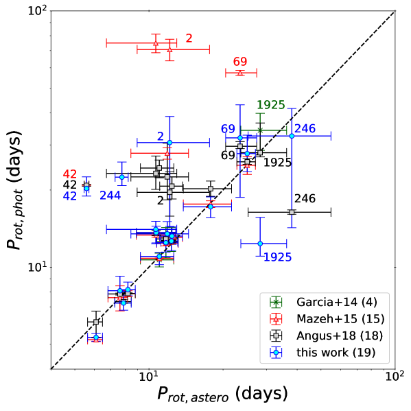
Figure 1: Photometric rotation periods $P_{\rm rot,phot}$ of the 19 planet-host stars against their asteroseismic rotation periods $P_{\rm rot,astero}$. The values of $P_{\rm rot,phot}$ are based on four independent papers as indicated in the legend. The number in the parenthesis indicates the number of stars plotted here that are overlapped in the paper and this work. We mark 6 stars, whose $P_{\rm rot,phot}$ derived from the LS periodogram is unreliable (bimodal or uncertain), by their KOI IDs (see Table 1).

Clearly, measured values of $P_{\rm rot,phot}$ published in literature are rather different, indicating that the measurements of $P_{\rm rot,phot}$ are somewhat dependent on the detailed methods of identifying the photometric variation. This is why discrepant values for the same systems are exhibited in some cases. In particular, we note that for $P_{\rm rot,astero}\approx 10-20$ days, the estimates by Angus et al. (2018) are larger by a factor $\approx 2$ (gray squares) relative to ours (blue circles). We individually examine the the LS periodogram of the 19 systems, and find that their estimates do not correspond to the highest peaks for most of the above cases.

As Angus et al. (2018) clearly mentioned, Gaussian Processes (GP) are prone to over-fitting and require a lot of care when setting the hyper-parameters and hyper-priors. Actually, our examination of the low frequency power spectrum suggests that the GP method picks up a time-scale consistent with that of the convective turnover expected for Sun-like stars (see e.g. Landin et al., 2010), rather than the stellar rotation period. Therefore, it is likely that the GP method is difficult to clearly distinguish the granulation noise (in the power spectrum it shows up as a pink noise, often referred to as the Harvey-like profile) from the signal corresponding to the stellar surface rotation.

Both our asteroseismic and photometric estimates are largely consistent with the result of Mazeh et al. (2015) plotted in red triangles, but there are three stars for which their auto-correlation method gives rotational periods of more than $\sim 60$ days. This could be due to our box-car smoothing of 50 days (see §2.2), but is statistically unexpected for a Sun-like star in the main sequence phase (see McQuillan et al., 2014, and our Fig 2 below). Therefore we suspect that they correspond to harmonics of the true rotation period, perhaps more visible in the auto-correlation function adopted by Mazeh et al. (2015) rather than in the LS periodogram.

Figure 2 shows $P_{\rm rot,astero}$ (red circles) estimated by asteroseismology and $P_{\rm rot,phot}$ (blue circles) estimated by LS periodogram for those 19 planet-host stars against the stellar effective temperature $T_{\rm eff}$. For comparison, the mean and 1$\sigma$ region of $P_{\rm rot}$ – $T_{\rm eff}$ from photometric variation analysis of $\simeq 34,000$ Kepler stars (McQuillan et al., 2014) are plotted as the thick black line and gray area, respectively.

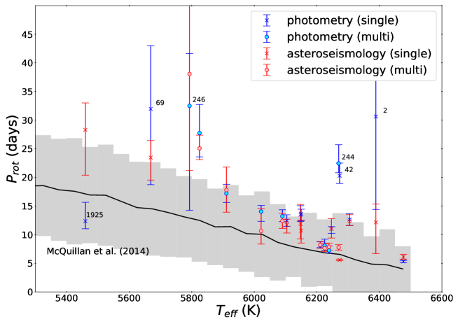
Figure 2: Rotation periods of the 19 stars against their effective temperature. Blue and red symbols correspond to $P_{\rm rot,phot}$ and $P_{\rm rot,astero}$ with crosses and circles indicating single and multiple planet systems, respectively. The mean and its 1$\sigma$ uncertainty regions for the photometrically derived rotation period (McQuillan et al., 2014) are plotted as the thick black line and the gray area. We mark 6 stars, whose $P_{\rm rot,phot}$ derived from the LS periodogram is unreliable by their KOI IDs.

Clearly both $P_{\rm rot,astero}$ and $P_{\rm rot,phot}$ measured by us for the 19 stars are systematically longer than the average of Kepler stars by McQuillan et al. (2014). As indicated by Figure 1, this tendency becomes even stronger if we plot $P_{\rm rot,phot}$ by Mazeh et al. (2015) and Angus et al. (2018). We also made sure that 48 planet-less stars with secure rotational period measurements from Kamiaka et al. (2018) exhibit the same trend, implying that the systematic tendency is not related to the effect of the accompanying planet.

The reason for this difference is unclear, but we suspect that this results from (unknown) factors affecting the detectability of solar-like pulsations. For example, magnetic activity is known to damp solar pulsations so that they show reduced amplitudes (e.g. Benomar et al., 2012). The statistical distribution derived by McQuillan et al. (2014), however, is still consistent at $2\sigma$ with our estimates, and thus the apparent discrepancy may be simply due to the limited size of our sample.

2.4 Validation of reliability of the stellar rotation periods

Figure 3: Examples of the LS periodogram for our sample. The thick black line indicates the boxcar-smoothed result (over 0.1 $\mu$Hz) of the original LS periodogram (thin gray curves). The original periodogram is normalized so that the maximum power of each system is unity. The period corresponding to the maximum power of the smoothed LS curve is marked by the vertical blue line, and the associated range of its full-width-at-half-maximum is plotted as blue-shaded areas. We also show the mean and its $1\sigma$ confidence interval of the asteroseismic rotation period by the horizontal red bar. Panel a. Example of reliable systems with a clear signature of the photometric rotation. Panels b and c. two bimodal systems (Kepler-25 and 410) that exhibit clear double peaks, neither of which match the asteroseismic rotation period.

Our LS periodogram analysis returns unusually large uncertainties for four KOIs (KOI 2, 69, 246, and 1925), and discrepant results compared to seismology for two KOIs (KOI 42 and 244), which are labeled in Figures 1 and 2. We carefully examine their LS periodogram, and consider the origin of these discrepancies as described in what follows.

Figure 3a shows the LS periodogram for KOI-1612 (Kepler-408) whose highest peak (blue area) is consistent with the period estimated from asteroseismology (red bars); 13 out of the 19 systems belong to this case, and will be referred to as reliable. We note also that Kepler-408b is the smallest planet ever discovered to be in a significantly misaligned orbit (Kamiaka et al., 2019).

Figure 3b and c plots the LS periodogram for the two stars classified as bimodal, , KOI-244 (Kepler-25) and KOI-42 (Kepler-410), which exhibit a discrepancy between seismology and the LS periodogram analysis. We note that they have two clear peaks in the LS periodogram, neither of which agrees with the seismic rotation period.

We do not yet understand the origin of this bimodality nor discrepancy. It may indicate that the transit signal is not completely removed during the lightcurve preparation, and that the residual contaminates the periodogram. It seems more likely, however, that the peaks are related to some harmonics of the true rotation period, while the true period itself is obscured for some unknown reason. Indeed $P_{\rm rot,phot}$ corresponding to the highest peak in the periodogram are $\approx 3P_{\rm rot,astero}$ and $\approx 4P_{\rm rot,astero}$ for KOI-244 and KOI-42, respectively.

The remaining four systems, referred to as uncertain, KOI-2, 246, 69 and 1925, do not show any clear peak in the LS periodogram. We cannot estimate the rotation period of those stars due to the large uncertainty. This may be partly because the star is significantly inclined with respect to the line-of-sight, or partly because the star has a weak magnetic activity level. For cool stars that are supposed to exhibit detectable star-spot activity, therefore, such transiting planetary systems with no clear peak in the periodogram may be good candidates for oblique systems. This will be discussed further in subsection 3.1 below.

3 Implications

3.1 Constraints on stellar inclination and frequency splitting from asteroseismology

In order to see if the four uncertain stars indeed correspond to oblique (low inclination) systems, we compute constraints on their stellar inclination and the rotational splitting $\delta\nu_{\star}$ from asteroseismic analysis. Further details of the analysis are described in Kamiaka et al. (2018, 2019).

The top-right panels in Figures 4 to 7 show the posterior probability density (PPD) on $i_{\star}$ – $\delta\nu_{\star}$ plane, marginalized over the other model parameters. The corresponding one-dimensional marginalized densities of $\delta\nu_{\star}$ and $i_{\star}$ are plotted to the left and below the axes, respectively. Finally the bottom–left panel is the marginalized PPD of $\delta\nu_{\star}\sin{i_{\star}}$, which may be estimated independently from the spectroscopic analysis of the line profiles. The solid and dashed lines in the one-dimensional marginalized PPD indicate the median and the associated 68% credible ranges, respectively.

If neither latitudinal nor radial differential rotation is present, the stellar rotation period is simply related to the rotational splitting $\delta\nu_{\star}$ estimated from asteroseismology as

$$P_{\rm rot}\approx 11.6\left(\frac{\mu{\rm Hz}}{\delta\nu_{\star}}\right){\rm days}.$$ (8)

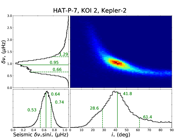
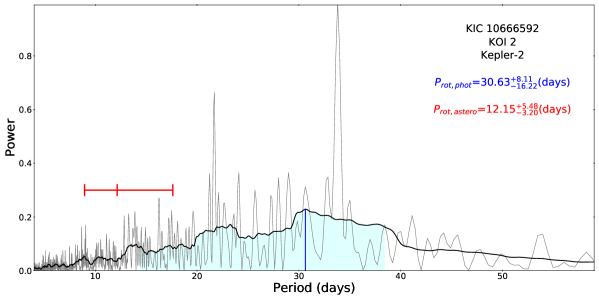
Figure 4: Constraints on the stellar inclination $i_{\star}$ and frequency splitting $\delta\nu_{\star}$ of KOI-2 (Kepler-2, HAT-P-7) from asteroseismic analysis. We plot the posterior probability density (PPD) on $i_{\star}$ – $\delta\nu_{\star}$ plane, marginalized over the other parameters. The one-dimensional marginalized densities are also shown to the left and below the axes. The bottom–left panel is the PPD of $\delta\nu_{\star}\sin{i_{\star}}$.

As Figures 4 to 7 indicate, $i_{\star}$ and $\delta\nu_{\star}$ ($=1/P_{\rm rot,astero}$) are strongly correlated in general. On the other hand, the asteroseismic analysis is known to be able to identify the value of $\delta\nu_{\star}\sin i_{\star}$ in a robust manner. Kamiaka et al. (2019) have presented the most comprehensive discussion on the joint analysis of asteroseismology and photometric variation for Kepler-408, one of the reliable stars in the present sample.

Unfortunately $P_{\rm rot,phot}$ for the uncertain stars are not reliable, and we cannot break the degeneracy precisely. Nevertheless, it is clear that they have systematically lower inclinations around $40^{\circ}$ than the reliable stars from asteroseismology alone, except Kepler-408 (see Table 1). This supports, at least qualitatively, our interpretation why they do not show any detectable periodicity in their photometric lightcurves.

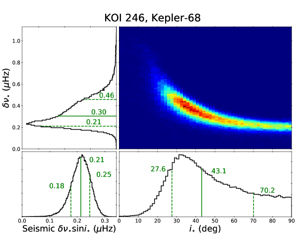
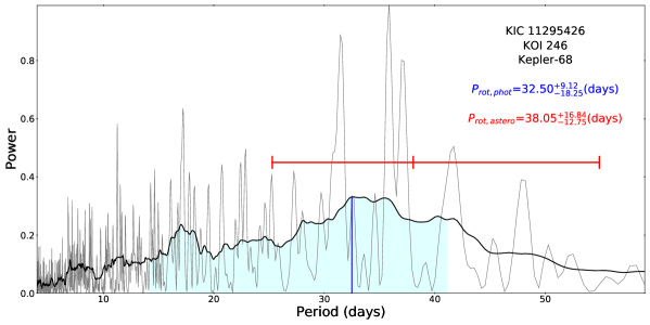
Figure 5: Same as Figure 4 but for KOI-246 (Kepler-68).

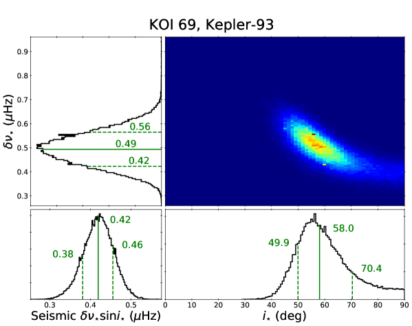
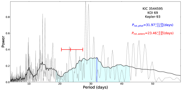
Figure 6: Same as Figure 4 but for KOI-69 (Kepler-93).

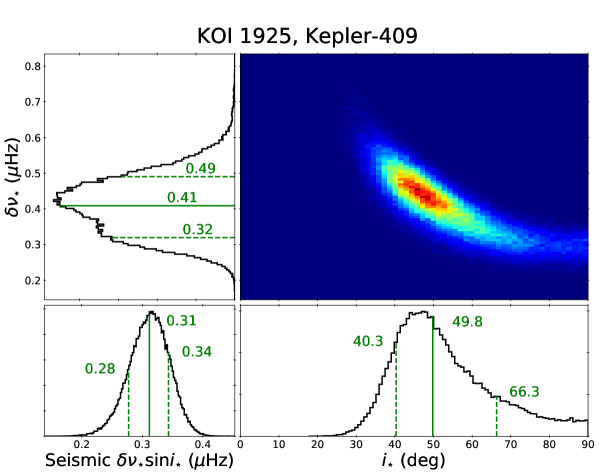
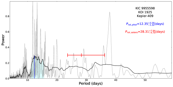
Figure 7: Same as Figure 4 but for KOI-1925 (Kepler-409).

In this context, we emphasize that a large projected spin-orbit misalignment of Kepler-2 (HAT-P-7) has already been discovered by Winn et al. (2009). Moreover, Benomar et al. (2014b) attempted for the first time to recover the full spin-orbit angle, instead of its projected value $\lambda$, through the joint analysis of the RM effect and asteroseismology. They considered two systems, HAT-P-7 (Kepler-2, Figure 4) and Kepler-25 (Figure 3b), which are classified here as uncertain and bimodal, respectively.

As in the case of Kepler-56 (Huber et al., 2013), the determination of the stellar inclination angles of Kepler-68 and Kepler-25 are of great value because they host more than one transiting planets. Kepler-68 has three planets, including two inner rocky planets ($R_{\rm p}=2.4R_{\oplus},1.0R_{\oplus}$) in compact, and possibly eccentric, orbits ($P_{\rm orb}=5.4$ days, $9.6$ days); see Table 3. Our analysis indicates that $i_{\star}=43.1^{+27.1}_{-15.1}$ and $80.6^{+6.6}_{-9.2}$ degrees for Kepler-68 and Kepler-25, respectively. While Kepler-68 could be another case for the strongly inclined multi-planetary system like Kepler-56, it is still consistent with $i_{\star}=90$ degrees as shown in Figure 5.

Kepler-93 has a close-in rocky planet ($R_{\rm p}=1.6R_{\oplus}$, $P_{\rm orb}=4.7$ days) and a massive planet in a distant orbit ($P_{\rm orb}>1460$ days). Kepler-409 has an Earth-sized planet ($R_{\rm p}=1.2R_{\oplus}$) in a 69-day orbit.

Because the measurement of the projected spin-orbit angle $\lambda$ for such small planets is practically impossible at this point, the above three systems may be new interesting candidates for obliquity studies based on asteroseismology, in particular Kepler-68 among others(Kamiaka et al., 2019).

It is also possible to constrain the value of $\delta\nu_{\star}\sin{i_{\star}}$ combining the stellar radius from the Kepler photometry and the sky-projected rotation velocity from the observed spectral line broadening. Adopting the spectroscopic measurement by Petigura et al. (2017) and Johnson et al. (2017), we find $\delta\nu_{\star}\sin{i_{\star}}=0.60{\pm}0.12$ $\mu$Hz for HAT-P-7 (Kepler-2), which is in good agreement with our asteroseismic result (Figure 4). HAT-P-7 is a well-known system with a large projected spin-orbit angle $\lambda$, and it is reasonable that the stellar spin is also significantly inclined towards us (Benomar et al., 2014b). On the contrary, the spectroscopic estimate of $\delta\nu_{\star}\sin{i_{\star}}=0.62{\pm}0.26$ $\mu$Hz for Kepler-409 is larger than our asteroseismic estimate, although barely consistent within 1-2 $\sigma$ (Figure 7). Thus Kepler-409 may be a well-aligned system. For the other two stars, Kepler-93 and 68, their line broadening widths are consistent with zero within an error of 1km/s (Petigura et al., 2017; Johnson et al., 2017), supporting our interpretation that they are significantly misaligned systems. Therefore those uncertain planet-host stars that exhibit no clear photometric variation deserve further detailed studies as good candidates of misaligned systems, in particular if their line broadening widths are unusually small.

3.2 Possible signature of (quasi-)spin-orbit resonance

Given the comparison of the different estimates of $P_{\rm rot,phot}$ described above, we decided to use our own results (blue circles in Figure 1) and $P_{\rm rot,astero}$ (Kamiaka et al., 2018) as the two independent proxies for the true rotation period in this subsection. Because we inspected the LS periodogram of the 19 systems individually and homogeneously, our estimate of $P_{\rm rot,phot}$ is more robust and reliable than those presented in the previous literature (Figure 1).

Before proceeding, we would like to stress here that strictly speaking, neither $P_{\rm rot,astero}$ nor $P_{\rm rot,phot}$ may represent the true rotation period of the star $P_{\rm rot,true}$. The surface differential rotation would lead to $P_{\rm rot,phot}>P_{\rm rot,true}$ for most stars in which the high-latitude surface rotates more slowly than the equator. Multiple formation/dissipation of star-spots may result in $P_{\rm rot,phot}/P_{\rm rot,true}$ significantly different from unity. It may be also the case for $P_{\rm rot,astero}$, which mainly probes the stellar internal rotation using its effect on stellar surface oscillations.

Taking account of a possibility that neither $P_{\rm rot,phot}$ nor $P_{\rm rot,astero}$ does not necessarily represent $P_{\rm rot,true}$, we select 13 stars (out the 19 stars excluding the two bimodal and four uncertain systems) satisfying $0.7<P_{\rm rot,phot}/P_{\rm rot,astero}<1.3$; see Tables 2 and 3. Thus their $P_{\rm rot,astero}$ and $P_{\rm rot,photo}$ may be regarded as a reasonably good proxy for $P_{\rm rot,true}$, while their quantitative difference needs to be kept in mind in understanding the result presented below.

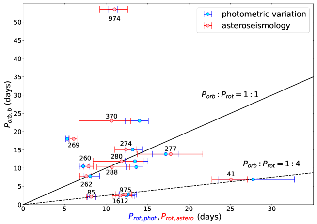
Figure 8: Orbital periods of the innermost planets $P_{\rm orb,b}$ plotted against the photometric and seismic stellar rotation periods, $P_{\rm rot,phot}$ (blue) and $P_{\rm rot,astero}$ (red). The number labeling the symbols indicates the KOI ID. Just for reference, $P_{\rm orb,b}/P_{\rm rot}$=1, and 1/4 are plotted in solid and dashed lines.

Figure 8 plots $P_{\rm orb,b}$ against $P_{\rm rot,phot}$ (blue) and $P_{\rm rot,astero}$ (red) for the 13 reliable systems. We identify a weak clustering around $P_{\rm orb,b}/P_{\rm rot}=1$ and $1/4$, especially for $P_{\rm rot,astero}$ that we assume to be more accurate and robust than $P_{\rm rot,phot}$.

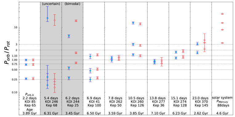
Figure 9: $P_{\rm orb}/P_{\rm rot,phot}$ (blue symbols) and $P_{\rm orb}/P_{\rm rot,astero}$ (red symbols) for multi-planetary systems. Systems without reliable $P_{\rm rot,phot}$ measurement are gray-shaded. Just for comparison, we plot the Solar system as well.

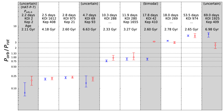
Figure 10: Same as Figure 9, but for for single-planet systems.

Figure 9 shows the trend more specifically and clearly perhaps, in which the overall spin-orbit architecture for multi-planetary systems is plotted separately. Interestingly and intriguingly, $P_{\rm orb}/P_{\rm rot}$ for seven multi-planetary systems (except bimodal or uncertain systems shaded as gray) does not seem to distribute in a homogeneous fashion, but rather preferentially takes discrete values approximated by simple integer ratios, including $P_{\rm orb}/P_{\rm rot}=1$. The most straightforward and bold interpretation is that those systems are in quasi-spin-orbit resonant states that have $P_{\rm orb}/P_{\rm rot}\approx n/m$ with $n$ and $m$ being simple integers.

Figure 10 is the same as Figure 9 but for single-planetary systems (six reliable systems together with three uncertain and one bimodal systems shaded as gray). Apart from the four stars classified as uncertain or bimodal, a possible (quasi-)spin-orbit resonance is still visible, even though to a lesser extent than exhibited in Figure 9. This may be simply a statistical fluctuation, but may also suggest that the apparent spin-orbit resonance is somehow related to, or even enhanced by the orbital resonance in the overall architecture of the multi-planetary systems.

A strong argument against the interpretation would come from the fact that the time-scale $\tau_{\rm sync}$ of the spin-orbit synchronization ($P_{\rm orb,b}/P_{\rm rot}\approx 1$) is unrealistically long at least in a conventional equilibrium tide model for a near-circular planetary orbit. Nevertheless we may speculate that there are a few dynamically stable local minima corresponding to $P_{\rm orb,b}/P_{\rm rot}\approx n/m$. In the course of the slow-down of the stellar rotation and/or the planetary migration that are not directly triggered by the tidal interaction, the star-planet system may be trapped in one of such quasi-resonant states temporarily. If this really happens, the corresponding time-scale could be significantly smaller than $\tau_{\rm sync}$ based on the mere tidal interaction. Otherwise the current result would challenge the existing tidal theories if it is not just a statistical fluke.

Figure 11: Posterior probability density (PPD) for $P_{\rm orb}/P_{\rm rot,astero}$ in logarithmic scale. Red and blue lines represent marginalized PPDs based on the inner-most planets alone ($N_{\rm planet}=13$) and on all the planets ($N_{\rm planet}=23$).

Because of the limited number of the planetary systems that allow a reliable asteroseismic estimate of the stellar rotation period, it is not easy to provide the statistical significance of the presence of the possible spin-orbit resonance. Nevertheless we attempt to evaluate it using the posterior probability density (PPD) for $P_{\rm rot,astero}$ obtained by Kamiaka et al. (2018). The result is plotted in Figure 11, which corresponds to the PPD of $x\equiv P_{\rm orb}/P_{\rm rot,astero}$ in the logarithmic scale normalized as

$$\int_{0}^{\infty}{\rm Prob}(x){\rm d}\log_{10}x=1.$$ (9)

The red and blue curves indicate the PPD for the inner-most and all planets, $N_{\rm planet}=13$ and 23, respectively, for the reliable systems alone. The vertical dotted lines indicate ratios of simple integers, which may be rather subjective but useful for reference.

We note here that even if the spin-orbit resonance interpretation is correct, $P_{\rm orb}/P_{\rm rot,astero}$ does not have to coincide with a ratio of simple integers exactly as already noted in the above. A possible radial differential rotation would make $P_{\rm rot,astero}$ slightly different from $P_{\rm rot,true}$. Furthermore, if the planetary orbit is eccentric, the stellar rotation velocity would be more likely synchronized towards the planetary orbital velocity at the pericenter. Thus $P_{\rm rot,true}$ may well differ from $P_{\rm orb}$ to some extent.

3.3 Discussion

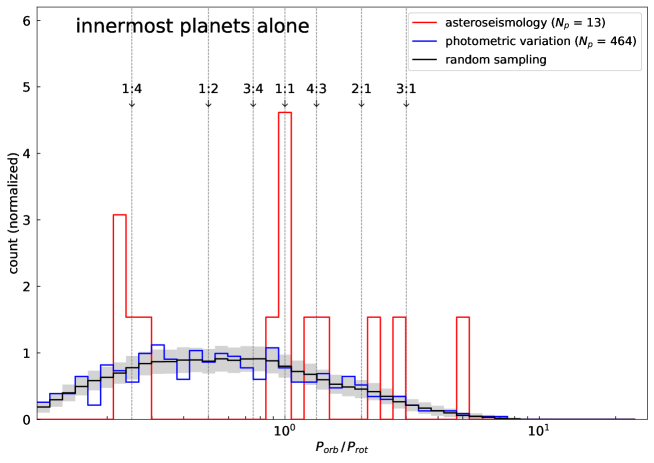
Figure 12: Histograms of $P_{\rm orb,b}/P_{\rm rot,astero}$ for our 13 reliable samples with $P_{\rm rot,astero}\approx P_{\rm rot,photo}$. The ratio is computed from the mean value of $P_{\rm rot,astero}$ with the logarithmically equal bin of 0.05.

We also attempt to compute the chance probability that 3 out of 13 stars have $0.96<P_{\rm orb,b}=P_{\rm rot}<1.02$; see KOI-262 (Kepler-50), KOI-280 (Kepler-1655) and KOI-288 in Tables 2 and 3. For that purpose, we adopt the data-set of the photometric stellar rotation period for 464 Kepler transiting planetary systems compiled by Mazeh et al. (2015). Figure 12 shows the corresponding normalized histogram of the ratio of central values of $P_{\rm orb,b}$ and $P_{\rm rot,phot}$ in blue. Then we randomly shuffle those values of $P_{\rm orb,b}$ and $P_{\rm rot,phot}$ in the systems. The average and $1\sigma$ region of 1000 sets of random sampling are plotted in black line and gray shaded area in Figure 12. We find that the fraction of a system having $0.96<P_{\rm orb,b}/P_{\rm rot,phot}<1.02$ is $p_{1}=2.12\%$. Thus the chance probability that 3 out of 13 stars have $0.96<P_{\rm orb,b}/P_{\rm rot,phot}<1.02$ is $p_{3}={}_{3}C_{13}p^{3}(1-p)^{10}\approx 0.22\%$. If we consider a broader range of $0.9<P_{\rm orb,b}/P_{\rm rot,phot}<1.1$ to take account of the associated errors, we find that $p_{1}=6.96\%$ and $p_{3}=4.68\%$. While these estimates should be still regarded as qualitative, instead of quantitative, they are helpful in interpreting the statistical significance of the current result.

Figure 13 plots the stellar parameters for the 13 reliable systems against $P_{\rm orb,b}/P_{\rm rot,astero}$. Due to the limited number of those systems, it is not easy to identify any statistical trend, but the three systems with $P_{\rm orb,b}/P_{\rm rot,astero}\approx 1$ may have similar effective temperature $T_{\rm eff}\approx 6200$K if at all.

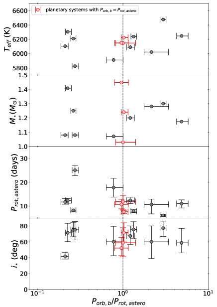
Figure 13: $T_{\rm eff}$, $M_{\star}$, $P_{\rm rot,astero}$ and $i_{\star}$ of the 13 planetary host stars against $P_{\rm orb,b}/P_{\rm rot,astero}$. All the quoted error-bars represent the 68% confidence level.

Finally we plot the spin-orbit angles $\lambda$ and $90^{\circ}-i_{\star}$ against $\tau_{\rm sync}$ in Figure 14 (see also Figure 12 of Kamiaka et al., 2019). The black symbols refer to $\lambda$ from the RM database (Southworth, 2011), while the red symbols are based on our asteroseismic analysis (Kamiaka et al., 2018). As discussed in Introduction, the bimodal distribution of $\lambda$ in Figure 14 may suggest the presence of both primordial and realignment channels for the spin-orbit angle. If those systems around $\lambda\approx 0^{\circ}$ result from the realignment channel, at least partially, it also points to stronger tidal interaction because $\tau_{\rm sync}$ of the conventional equilibrium tide is too long. This may be the same puzzle that we encounter here in our interpretation of the possible spin-orbit resonance.

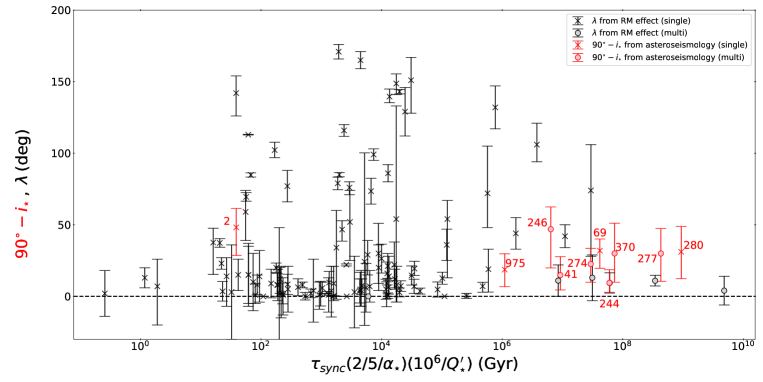
Figure 14: Spin-orbit angles $\lambda$ and $90^{\circ}-i_{\star}$ against $\tau_{\rm sync}$. The data for $\lambda$ for 124 transiting systems on the basis of the Rossiter-McLaughlin effect in black are taken from the compilation by Southworth (2011). Red symbols correspond to 10 systems from our own asteroseismic analysis (Kamiaka et al., 2018) with a planetary mass estimate. Crosses and circles indicate the single- and multi-planetary systems, respectively. The quoted error-bars represent the 68% credible interval.

4 Summary and Conclusion

We have performed asteroseismic analysis of 19 host stars in Kepler transiting planetary systems, and measured their rotation period $P_{\rm rot,astero}$. We systematically compared our measurement against the photometric rotation period $P_{\rm rot,phot}$ estimated in previous literature (García et al., 2014; Mazeh et al., 2015; Angus et al., 2018) and also from our own Lomb-Scargle periodogram method.

In order to select a robust sample of stars with a reliable rotation period, we focused on stars that show consistent results between asteroseismic analysis and the LS periodogram. This turned out to be particularly important because we found a relatively low-level of agreement among different published values of $P_{\rm rot,phot}$; asteroseismology has played a key role in providing an entirely independent measurement of the stellar rotation. It is worth noting that a careful case-by-case examination is necessary if we use photometric variations (such as the LS periodogram) to derive $P_{\rm rot,phot}$. Indeed, the latitudinal differential rotation, the size of the star-spots and their typical formation/dissipation timescales would introduce significant differences between $P_{\rm rot,phot}$ and $P_{\rm rot,true}$.

Furthermore, the planet itself induces a photometric modulation that, if not entirely removed, could be incorrectly identified as the stellar rotation period. These issues can only be circumvented by checking results independently with different methods, such as presented in this study. Unfortunately, however, measuring the rotation with seismology requires high quality photometric data, so that it is difficult to increase the number of reliable stars significantly.

We found that 13 stars have a strong single peak in the periodogram and satisfy $0.7<P_{\rm rot,phot}/P_{\rm rot,astero}<1.3$, implying their rotation period is reliable because $P_{\rm rot,phot}$ and $P_{\rm rot,astero}$ do not have to be exactly the same due to the longitudinal and radial differential rotation. The photometric lightcurves for the remaining six systems exhibit either multiple peaks (two systems) or no clear peak (four systems) in the periodogram, and the resulting estimate of $P_{\rm rot,phot}$ is not reliable. This suggests that the photometrically determined stellar rotation period needs to be examined carefully on an individual basis.

While the fraction of stars with measured $P_{\rm rot,astero}$ is relatively small, detailed comparison of their $P_{\rm rot,phot}$ and $P_{\rm rot,astero}$ is useful in calibrating the reliability of $P_{\rm rot,phot}$, and also exploring the spin-orbit architecture of planetary systems in a robust fashion.

One straightforward application is the determination of the stellar inclination $i_{\star}$. The asteroseismic estimate of $i_{\star}$ for the 13 reliable stars can be more accurate and/or precise with the joint analysis with $P_{\rm rot,phot}$. A notable example includes Kepler-408b, the smallest planet known to have a significantly misaligned orbit with $i_{\star}=42^{+5}_{-4}$ degrees (Kamiaka et al., 2019). The four uncertain systems, Kepler-2, 68, 93 and 409, may also be good candidates that host mis-aligned planets.

Another interesting possibility that we discussed in this paper is the correlation between the stellar rotation period and the orbital periods of accompanying planets. Among the 13 reliable systems, we found that three inner-most planets, KOI-262b, 280b, 288b, have $0.96<P_{\rm orb,b}/P_{\rm rot,astero}<1.02$. On the basis of 464 systems with photometric stellar periods, we estimate that the corresponding chance probability is ($0.2$ – $5$) % depending on the assumption.

Since the statistical significance for the spin-orbit resonance is admittedly not so strong, a larger sample of stars would be required to confirm/refute our current result. Nevertheless, if confirmed, the (quasi-)spin-orbit resonance points towards a strong tidal interaction between stars and planets. This cannot be explained in a conventional equilibrium tide model. Due to the limited number of planetary systems with a reliable stellar rotation period, the interpretation of the current data is not conclusive yet. Further investigation on the basis of the carefully examined photometric variation analysis is of great importance, which we plan to pursue and report in due course.

Table 1: Basic stellar properties of 19 planetary systems; $T_{\rm eff}$ and $P_{\rm rot,phot}$ denote the effective temperature and photometrically-derived rotation period. The seismically derived rotation period, $P_{\rm rot,astero}$, and inclination, $i_{\star,\rm astero}$, are estimated using uniform priors, while $i_{\star,\rm joint}$ is derived using the photometric rotation period as a prior in the seismic analysis. The quoted errors correspond to the 68% credible intervals around the median value. The three systems in bold fonts correspond to those with $P_{\rm orb,b}\approx P_{\rm rot,astero}$.

KOI	Kepler ID	$T_{\rm eff}$	$P_{\rm rot,phot}$	$P_{\rm rot,astero}$	$i_{\star,\rm astero}$	$i_{\star,\rm joint}$
		(K)	(days)	(days)	(deg)	(deg)
Stars with reliable period measurement
41	100	5825	$27.7_{-4.2}^{+5.0}$	$25.1_{-2.3}^{+2.0}$	$75.2_{-12.9}^{+10.4}$	$77.6_{-11.1}^{+8.6}$
85	65	6211	$8.2_{-0.4}^{+0.6}$	$8.2_{-0.6}^{+0.6}$	$75.0_{-8.7}^{+9.5}$	$75.4_{-7.7}^{+9.0}$
260	126	6239	$7.2_{-0.5}^{+0.8}$	$7.9_{-0.6}^{+0.6}$	$75.6_{-11.2}^{+9.7}$	$73.8_{-10.2}^{+10.4}$
262	50	6225	$8.1_{-0.8}^{+1.1}$	$7.6_{-0.8}^{+0.6}$	$71.6_{-11.7}^{+12.3}$	$75.1_{-10.6}^{+9.9}$
269	…	6477	$5.3_{-0.2}^{+0.2}$	$6.1_{-0.5}^{+0.4}$	$77.3_{-10.5}^{+8.7}$	$66.0_{-5.5}^{+7.5}$
274	128	6090	$13.2_{-0.9}^{+1.1}$	$12.4_{-1.3}^{+1.3}$	$67.4_{-10.9}^{+12.7}$	$71.5_{-8.4}^{+10.7}$
277	36	5911	$17.2_{-1.6}^{+1.6}$	$17.8_{-4.0}^{+3.9}$	$60.0_{-17.5}^{+19.4}$	$62.4_{-12.7}^{+16.2}$
280	1655	6148	$13.5_{-1.2}^{+1.6}$	$11.9_{-3.4}^{+2.6}$	$58.9_{-17.7}^{+18.8}$	$68.3_{-11.9}^{+13.3}$
288	…	6150	$13.6_{-1.2}^{+0.8}$	$10.7_{-1.8}^{+2.2}$	$52.2_{-9.5}^{+13.1}$	$67.1_{-9.6}^{+13.0}$
370	145	6022	$14.0_{-1.7}^{+1.1}$	$10.7_{-3.9}^{+2.3}$	$60.0_{-21.1}^{+20.1}$	$78.1_{-11.6}^{+8.2}$
974	…	6247	$11.0_{-0.8}^{+0.4}$	$11.0_{-1.8}^{+1.6}$	$58.7_{-12.6}^{+18.2}$	$62.1_{-8.3}^{+12.4}$
975	21	6305	$12.6_{-1.0}^{+1.0}$	$12.3_{-1.2}^{+0.8}$	$71.3_{-11.0}^{+12.0}$	$75.1_{-8.8}^{+9.8}$
1612	408	6104	$12.5_{-1.0}^{+1.0}$	$11.7_{-1.0}^{+1.4}$	$41.7_{-3.5}^{+5.1}$	$43.1_{-2.9}^{+3.5}$
Stars with no clear signal in periodogram
2	2	6389	$30.6_{-16.2}^{+8.1}$	$12.1_{-3.2}^{+5.5}$	$41.8_{-13.2}^{+19.6}$	…
69	93	5669	$32.0_{-13.2}^{+11.0}$	$23.5_{-3.0}^{+3.9}$	$58.0_{-8.1}^{+12.3}$	…
246	68	5793	$32.5_{-18.2}^{+9.1}$	$38.0_{-12.8}^{+16.8}$	$43.1_{-15.5}^{+27.1}$	…
1925	409	5460	$12.4_{-1.3}^{+3.3}$	$28.3_{-4.7}^{+7.9}$	$49.8_{-9.5}^{+16.5}$	…
Stars with bimodal peaks in periodogram
42	410	6273	$20.3_{-1.3}^{+2.2}$	$5.6_{-0.1}^{+0.1}$	$83.6_{-5.2}^{+4.4}$	…
244	25	6270	$22.4_{-1.6}^{+3.3}$	$7.8_{-0.5}^{+0.5}$	$80.6_{-9.2}^{+6.6}$	…

References: $T_{\rm eff}$ is from NASA Exoplanet Archive (https://exoplanetarchive.ipac.caltech.edu).

Table 2: Properties of single-planetary systems.

KOI	Kepler ID	$R_{\rm p}$	$M_{\rm p}$	$e$	$a$	$P_{\rm orb}$	$P_{\rm orb}/P_{\rm rot,phot}$	$P_{\rm orb}/P_{\rm rot,astero}$
		($R_{\oplus}$)	($M_{\oplus}$)		(au)	(days)
Stars with reliable period measurement
269	…	1.83	…	…	0.15	18.01	$3.38_{-0.11}^{+0.12}$	$2.95_{-0.17}^{+0.24}$
280	1655	2.21	5.0	…	0.10	11.87	$0.88_{-0.09}^{+0.08}$	$1.00_{-0.18}^{+0.41}$
288	…	3.04	…	…	0.10	10.28	$0.75_{-0.04}^{+0.07}$	$0.96_{-0.16}^{+0.20}$
974	…	2.52	…	…	0.29	53.51	$4.86_{-0.17}^{+0.37}$	$4.86_{-0.62}^{+0.94}$
975	21	1.64	5.08	0.02	0.04	2.79	$0.22_{-0.02}^{+0.02}$	$0.23_{-0.01}^{+0.02}$
1612	408	0.82	…	…	…	2.47	$0.20_{-0.01}^{+0.02}$	$0.21_{-0.02}^{+0.02}$
Stars with no clear signal in periodogram
2	2	16.9	585	…	0.04	2.20	$0.07_{-0.02}^{+0.08}$	$0.18_{-0.06}^{+0.06}$
69	93	1.6	3.2	…	0.05	4.73	$0.15_{-0.04}^{+0.10}$	$0.20_{-0.03}^{+0.03}$
1925	409	1.19	…	…	…	68.96	$5.58_{-1.18}^{+0.67}$	$2.44_{-0.53}^{+0.48}$
Stars with bimodal peaks in periodogram
42	410	2.84	…	0.17	0.12	17.83	$0.88_{-0.09}^{+0.06}$	$3.20_{-0.07}^{+0.07}$

References: $R_{\rm p}$, $M_{\rm p}$, $e$, $a$, and $P_{\rm orb}$ are from NASA Exoplanet Archive (https://exoplanetarchive.ipac.caltech.edu).

Table 3: Properties of multi-planetary systems.

KOI	Kepler ID	$R_{\rm p}$	$M_{\rm p}$	$e$	$a$	$P_{\rm orb}$	$P_{\rm orb}/P_{\rm rot,phot}$	$P_{\rm orb}/P_{\rm rot,astero}$
		($R_{\oplus}$)	($M_{\oplus}$)		(au)	(days)
Stars with reliable period measurement
41	100	1.32	7.34	0.13	…	6.89	$0.25_{-0.04}^{+0.04}$	$0.27_{-0.02}^{+0.03}$
		2.20	…	0.02	…	12.82	$0.46_{-0.07}^{+0.08}$	$0.51_{-0.04}^{+0.05}$
		1.61	…	0.02	…	35.33	$1.27_{-0.19}^{+0.22}$	$1.41_{-0.10}^{+0.14}$
85	65	1.42	…	0.02	0.04	2.15	$0.26_{-0.02}^{+0.01}$	$0.26_{-0.02}^{+0.02}$
		2.58	26.6	0.08	0.07	5.86	$0.72_{-0.05}^{+0.04}$	$0.71_{-0.05}^{+0.06}$
		1.52	…	0.10	0.08	8.13	$1.00_{-0.07}^{+0.06}$	$0.99_{-0.07}^{+0.08}$
260	126	1.52	…	0.07	0.10	10.50	$1.45_{-0.14}^{+0.10}$	$1.33_{-0.09}^{+0.11}$
		1.58	…	0.19	0.16	21.87	$3.02_{-0.30}^{+0.20}$	$2.77_{-0.19}^{+0.24}$
		2.50	…	0.02	0.45	100.28	$13.84_{-1.37}^{+0.92}$	$12.72_{-0.89}^{+1.09}$
262	50	1.71	…	…	0.08	7.81	$0.97_{-0.12}^{+0.11}$	$1.02_{-0.07}^{+0.12}$
		2.17	…	…	0.09	9.38	$1.16_{-0.14}^{+0.14}$	$1.23_{-0.08}^{+0.15}$
274	128	1.13	30.7	…	0.13	15.09	$1.14_{-0.09}^{+0.09}$	$1.22_{-0.12}^{+0.15}$
		1.13	33.3	…	0.17	22.80	$1.73_{-0.14}^{+0.13}$	$1.84_{-0.18}^{+0.22}$
277	36	1.49	4.45	0.04	0.12	13.84	$0.80_{-0.07}^{+0.08}$	$0.78_{-0.14}^{+0.23}$
		3.68	8.08	…	0.13	16.24	$0.94_{-0.08}^{+0.10}$	$0.91_{-0.16}^{+0.27}$
370	145	2.65	37.1	0.43	…	22.95	$1.63_{-0.12}^{+0.23}$	$2.15_{-0.38}^{+1.26}$
		4.32	79.4	0.11	…	42.88	$3.05_{-0.22}^{+0.42}$	$4.02_{-0.71}^{+2.36}$
Stars with no clear signal in periodogram
246	68	2.40	6.00	…	0.06	5.40	$0.17_{-0.04}^{+0.21}$	$0.14_{-0.04}^{+0.07}$
		1.00	4.80	0.42	0.09	9.61	$0.30_{-0.06}^{+0.38}$	$0.25_{-0.08}^{+0.13}$
		…	267	0.18	1.40	625	$19.23_{-4.22}^{+24.63}$	$16.43_{-5.04}^{+8.28}$
Stars with bimodal peaks in periodogram
244	25	2.71	9.60	…	0.07	6.24	$0.28_{-0.04}^{+0.02}$	$0.80_{-0.05}^{+0.05}$
		5.20	24.60	0.01	0.11	12.72	$0.57_{-0.07}^{+0.04}$	$1.64_{-0.09}^{+0.11}$
		…	89.90	…	…	123	$5.48_{-0.70}^{+0.43}$	$15.83_{-0.90}^{+1.04}$

References: $R_{\rm p}$, $M_{\rm p}$, $e$, $a$, and $P_{\rm orb}$ are from NASA Exoplanet Archive (https://exoplanetarchive.ipac.caltech.edu).

References

- Albrecht et al. (2012) Albrecht, S., Winn, J. N., Johnson, J. A., et al. 2012, ApJ, 757, 18
- Angus et al. (2018) Angus, R., Morton, T., Aigrain, S., Foreman-Mackey, D., & Rajpaul, V. 2018, MNRAS, 474, 2094
- Benomar et al. (2012) Benomar, O., Baudin, F., Chaplin, W. J., Elsworth, Y., & Appourchaux, T. 2012, MNRAS, 420, 2178
- Benomar et al. (2014a) Benomar, O., Masuda, K., Shibahashi, H., & Suto, Y. 2014a, PASJ, 66, 94
- Benomar et al. (2014b) Benomar, O., Belkacem, K., Bedding, T. R., et al. 2014b, ApJ, 781, L29
- Benomar et al. (2018) Benomar, O., Bazot, M., Nielsen, M. B., et al. 2018, Science, 361, 1231
- Campante et al. (2016) Campante, T. L., Lund, M. N., Kuszlewicz, J. S., et al. 2016, ApJ, 819, 85
- Chaplin et al. (2013) Chaplin, W. J., Sanchis-Ojeda, R., Campante, T. L., et al. 2013, ApJ, 766, 101
- García et al. (2014) García, R. A., Ceillier, T., Salabert, D., et al. 2014, A&A, 572, A34
- Gizon & Solanki (2003) Gizon, L., & Solanki, S. K. 2003, ApJ, 589, 1009
- Gratia & Fabrycky (2017) Gratia, P., & Fabrycky, D. 2017, MNRAS, 464, 1709
- Huber et al. (2013) Huber, D., Carter, J. A., Barbieri, M., et al. 2013, Science, 342, 331
- Johnson et al. (2017) Johnson, J. A., Petigura, E. A., Fulton, B. J., et al. 2017, AJ, 154, 108
- Kamiaka et al. (2018) Kamiaka, S., Benomar, O., & Suto, Y. 2018, MNRAS, 479, 391
- Kamiaka et al. (2019) Kamiaka, S., Benomar, O., Suto, Y., et al. 2019, arXiv e-prints, arXiv:1902.02057
- Lai (2012) Lai, D. 2012, MNRAS, 423, 486
- Landin et al. (2010) Landin, N. R., Mendes, L. T. S., & Vaz, L. P. R. 2010, A&A, 510, A46
- Lurie et al. (2017) Lurie, J. C., Vyhmeister, K., Hawley, S. L., et al. 2017, AJ, 154, 250
- Mazeh et al. (2015) Mazeh, T., Perets, H. B., McQuillan, A., & Goldstein, E. S. 2015, ApJ, 801, 3
- McLaughlin (1924) McLaughlin, D. B. 1924, ApJ, 60, 22
- McQuillan et al. (2014) McQuillan, A., Mazeh, T., & Aigrain, S. 2014, ApJS, 211, 24
- Murray & Dermott (2000) Murray, C. D., & Dermott, S. F. 2000
- Nagasawa et al. (2008) Nagasawa, M., Ida, S., & Bessho, T. 2008, ApJ, 678, 498
- Ohta et al. (2005) Ohta, Y., Taruya, A., & Suto, Y. 2005, ApJ, 622, 1118
- Petigura et al. (2017) Petigura, E. A., Howard, A. W., Marcy, G. W., et al. 2017, AJ, 154, 107
- Queloz et al. (2000) Queloz, D., Eggenberger, A., Mayor, M., et al. 2000, A&A, 359, L13
- Rogers & Lin (2013) Rogers, T. M., & Lin, D. N. C. 2013, ApJ, 769, L10
- Rossiter (1924) Rossiter, R. A. 1924, ApJ, 60, 15
- Southworth (2011) Southworth, J. 2011, ArXiv e-prints, arXiv:1108.2976
- Toutain & Gouttebroze (1993) Toutain, T., & Gouttebroze, P. 1993, A&A, 268, 309
- Winn et al. (2009) Winn, J. N., Johnson, J. A., Albrecht, S., et al. 2009, ApJ, 703, L99 (W09)
- Winn et al. (2005) Winn, J. N., Noyes, R. W., Holman, M. J., et al. 2005, ApJ, 631, 1215
- Winn et al. (2017) Winn, J. N., Petigura, E. A., Morton, T. D., et al. 2017, AJ, 154, 270
- Xue et al. (2014) Xue, Y., Suto, Y., Taruya, A., et al. 2014, ApJ, 784, 66