Optimal (Randomized) Parallel Algorithms
in the Binary-Forking Model

Abstract

In this paper we develop optimal algorithms in the binary-forking model for a variety of fundamental problems, including sorting, semisorting, list ranking, tree contraction, range minima, and ordered set union, intersection and difference. In the binary-forking model, tasks can only fork into two child tasks, but can do so recursively and asynchronously. The tasks share memory, supporting reads, writes and test-and-sets. Costs are measured in terms of work (total number of instructions), and span (longest dependence chain).

The binary-forking model is meant to capture both algorithm performance and algorithm-design considerations on many existing multithreaded languages, which are also asynchronous and rely on binary forks either explicitly or under the covers. In contrast to the widely studied PRAM model, it does not assume arbitrary-way forks nor synchronous operations, both of which are hard to implement in modern hardware. While optimal PRAM algorithms are known for the problems studied herein, it turns out that arbitrary-way forking and strict synchronization are powerful, if unrealistic, capabilities. Natural simulations of these PRAM algorithms in the binary-forking model (i.e., implementations in existing parallel languages) incur an $\Omega(\log n)$ overhead in span. This paper explores techniques for designing optimal algorithms when limited to binary forking and assuming asynchrony. All algorithms described in this paper are the first algorithms with optimal work and span in the binary-forking model. Most of the algorithms are simple. Many are randomized.

1 Introduction

In this paper we present several results on the binary-forking model. The model assumes a collection of threads that can be created dynamically and can run asynchronously in parallel. Each thread acts like a standard random-access machine (RAM), with a constant number of shared registers and sharing a common main memory. The model includes a fork instruction that forks an asynchronous child thread. A computation starts with a single thread and finishes when all threads end. In addition to reads and writes to the shared memory, the model includes a test-and-set (TS) instruction. Costs are measured in terms of the work (total number of instructions executed among all threads) and the span (the longest sequence of dependent instructions).

The binary-forking model is meant to capture the performance of algorithms on modern multicore shared-memory machines. Variants of the model have been widely studied [50, 3, 1, 26, 20, 33, 34, 24, 30, 31, 23, 32, 45, 42, 89, 54, 41]. They are also widely used in practice, and supported by programming systems such as Cilk [60], the Java fork-join framework [74], X10 [40], Habanero [38], Intel Threading Building Blocks (TBB) [71], and the Microsoft Task Parallel Library [91].

The binary forking model and variants are practical on multicore shared-memory machines in part because they are mostly asynchronous, and in part due to the dynamic binary forking. Asynchrony is important because the processors (cores) on modern machines are themselves highly asynchronous, due to varying delays from cache misses, processor pipelines, branch prediction, hyper-threading, changing clock speeds, interrupts, the operating system scheduler, and several other factors. Binary forking is important since it allows for efficient scheduling in both theory and practice, especially in the asynchronous setting [34, 25, 11, 2]. Efficient scheduling can be achieved even when the number of available processors changes over time [11], which often happens in practice due to shared resources, background jobs, or failed processors.

Due to these considerations, it would seem that these models are more practical for designing parallel algorithms than the more traditional PRAM model [86], which assumes strict synchronization on each step, and a fixed number of processors. One can also argue that they are a more convenient model for designing parallel algorithms, allowing, for example, the easy design of parallel divide-and-conquer algorithms, and avoiding the need to schedule by hand [19]. The PRAM can be simulated on the binary-forking model by forking $P$ threads in a tree for each step of the PRAM. However, this has a $O(\log n)$ overhead in span. This means that algorithms that are optimal on the PRAM are not necessarily optimal when mapped to the binary-forking model. For example, Cole’s ingenious pipelined merge sort on $n$ keys and processors takes optimal $O(\log n)$ parallel time (span) on the PRAM [43], but requires $O(\log^{2}n)$ span in the binary-forking model due to the cost of synchronization. On the other hand a $O(n\log n)$ work and $O(\log n\log\log n)$ span algorithms in the binary-forking model is know [45]. Therefore finding more efficient direct algorithms for the binary-forking model is an interesting problem. Known results are outlined in Section 1.1.

The variants of the binary-forking model differ in how they synchronize. The most common variant is binary fork-join model where every fork corresponds to a later join, and the fork and corresponding joins are properly nested [50, 1, 26, 33, 34, 30, 23, 45]. Other models allow more powerful synchronization primitives  [31, 42, 89, 54, 41, 11]. In this paper we allow a test-and-set (TS), which is a memory operation that atomically checks if a memory location is zero, returning the result, and sets it to one. This seems to give some power over the pure fork-join model. We make use of the TS in many of our algorithms. We justify including a TS instruction by noting that all modern multicore hardware includes the instruction. Furthermore all existing theoretical and practical implementations of the fork-join model require the test-and-set, or equivalently powerful operation to implement the join.

In this paper we describe several algorithms for fundamental problems that are optimal in both work and span in the binary-forking model. In particular, we show the following results.

Theorem 1.1 (Main Theorem).

Sorting, semisorting, list/tree contraction, random permutation, ordered-set operations, and range minimum queries can be computed in the binary-forking model with optimal work and 0pt ($O(\log n)$). In many cases the algorithms are randomized, as summarized in Table 1.

Problem		Work	Span
List Contraction	Sec 3	$O(n)$	$O(\log n)^{*}$
Sorting	Sec 4	$O(n\log n)^{\dagger}$	$O(\log n)^{*}$
Semisorting	Sec 4	$O(n)^{\dagger}$	$O(\log n)^{*}$
Random Permutation	Sec 6	$O(n)^{\dagger}$	$O(\log n)^{*}$
Range Minimum Query	Sec 7	$O(n)$	$O(\log n)$
Tree Contraction	Sec 8	$O(n)$	$O(\log n)^{*}$
Ordered-Set Operations	Sec 5	$O(m\log(\frac{n}{m}+1))$	$O(\log n)$
(Union, Intersect, Diff.)

Table 1: The bounds of our new algorithms in the binary-forking model. For ordered-set operations, $n$ and $m\leq n$ are sizes of two sets. $*$: with high probability (whp).  $\dagger$: in expectation. Bounds without superscripts are worst-case bounds. The ordered-set algorithms can work in binary-forking model only with join supported (either by using TS or just as a default primitive), and the rest make use of TS.

To achieve these bounds, we develop interesting algorithmic approaches. For some of them, we are inspired by recent results on identifying dependences in sequential iterative algorithms [22, 27, 87]. This paper discusses a non-trivial approach to convert the dependence DAG into an algorithm in the binary-forking model while maintaining the span of the algorithm to be the same as the longest chain in the DAG. This leads to particularly simple algorithms, even compared to previous PRAM algorithms whose span is suboptimal when translated to the binary-forking model. For some other algorithms, we use the $n^{\epsilon}$-way divide-and-conquer scheme. By splitting the problem into $n^{\epsilon}$ sub-problems and solving them in parallel in logarithmic time, we are able to achieve $O(\log n)$ span for the original problem. Our results on ordered sets are the best known (optimal work in the comparison model and $O(\log n)$ span) even when translated to other models such as the PRAM.

We note that for many of the problems we describe, it remains open whether the same bounds can be achieved deterministically, and also whether they can be achieved in the binary fork-join model without a TS. One could argue that avoiding a TS is more elegant.

1.1 Related Work

There have been many existing parallel algorithms designed based on variants of the binary-forking model (e.g., [3, 1, 26, 20, 24, 30, 31, 23, 32, 45, 42, 13, 89, 54, 41, 28, 53, 14, 52, 29]). Many of the results are in the setting of cache-efficient algorithms. This is because binary forking in conjunction with work-stealing or space-bounded schedulers leads to strong bounds on the number of cache misses on multiprocessors with various cache configurations [1, 42, 45, 23].

In the binary fork-join model, Blelloch et al. [26] give work-efficient $O(\log n)$ span algorithms for prefix sums and merging, and a work-efficient randomized sorting algorithm with $O(\log^{3/2}n)$ span whp. Cole and Ramachandran [45] improved this and gave a deterministic algorithm with span $O(\log n\log\log n)$. This is currently the best known result for sorting in the binary fork-join model, without a test-and-set, and also for deterministic sorting even with a test-and-set.

Allowing for more powerful synchronization, Blelloch et al. [30, 31] discussed how to implement futures using the TS instruction, which leads to some low-span binary-forking algorithms Tang et al. [89, 54, 41] described some dynamic programming algorithms, in the setting of cache efficiency. They also use a TS for synchronization. With this they can reduce the span of a variety of algorithms over fork-join computations without the atomic synchronizations. Without considering the additional support for cache efficiency, we believe their model is equivalent to the binary-forking model.

2 Models and Simulations

Here we describe the binary-forking model and its relationship to more traditional models of parallel computing, including the PRAM and circuit models. The binary-forking model falls into the class of multithreaded models [34, 25, 11, 44, 33]. Multithreaded computational models assume a collection of threads (sometimes called processes or tasks) that can be dynamically created, and generally run asynchronously. Cost is determined in terms of the total work and the computational span (also called depth or critical path length). There are several variants on multithreaded models depending on how many threads can be forked, how they synchronize, and assumptions about how the memory can be accessed. To be concrete, we define a specific model in this paper.

The binary-forking model.

The binary-forking model consists of threads that share a common memory. Each thread acts like a sequential RAM—it works on a program stored in the shared memory, has a constant number of registers (including a program counter), and has standard RAM instructions (including an end instruction to finish the computation). The binary-forking model extends the RAM with a fork instruction, which forks a child thread. We also employ a special end instruction named endall to indicate the completion of the whole computation. The fork instruction sets the first register to zero in the parent (forking) thread and to one in the child (forked) thread, to distinguish them. Otherwise the states of the threads are identical, including the program counter to the next instruction. As is standard with the sequential RAM [90], we assume that for input size $n$, all memory locations and registers can hold $O(\log n)$ bits.

In addition to reads and writes, we include a test-and-set (TS) instruction in the binary-forking model for accessing memory. The TS is an atomic instruction that reads a memory location and if the memory location is zero, sets it to one, returning zero. Otherwise it leaves the value unchanged returning one. We note that all currently produced processors support the TS instruction in hardware.

In a binary-forking model, a computation starts with a single initial thread and finishes when endall is called. The invocation to an endall can be determined by the algorithm, for example, through using TS instructions (e.g., to implement join instructions, see below). A computation in the binary-forking model can therefore be viewed as a tree where each node is an instruction with the next instruction as a child, and where the fork instruction has two children corresponding to the next instruction of the original forking thread and the first instruction of the forked thread. The root of the tree is the first instruction of the initial thread. We define the work of a computation as the size of the tree (total number of instructions) and the span as the depth of the tree (longest path of instructions). We assume the results of memory operations are consistent with some total order (linearization) of the instructions that preserves the partial order defined by the tree. For example, a read will return the value of the previous write or TS to the same location in the total order. The choice of total order can affect the results of a program since threads can communicate through the shared memory. In general, therefore, computations are nondeterministic.

To simplify issues of parallel memory allocation we assume there is an allocate instruction that takes a positive integer $n$ and allocates a contiguous block of $n$ memory locations, returning a pointer to the block, and a free instruction that given a pointer to an allocated block, frees it.

We use $\mathcal{BF}(W(n),S(n))$ to denote the class of algorithms that require $O(W(n))$ work and $O(S(n))$ span for inputs of size $n$ in the binary-forking model. We use $\mathcal{BF}^{k}$ when $S(n)=O(\log^{k}(n))$ and $W(n)$ is polynomial in $n$, and $\mathcal{BF}^{*}$ when the span is polylogarithmic and the work is polynomial.

The binary-forking model can be extended to support arbitrary-way forking instead of binary. In particular, the fork instruction can take an integer specifying the number of threads to fork, and each forked thread then gets a unique integer identifier in a register. The focus of this paper, however, is on binary forking since there are no known optimal scheduling results for arbitrary-way forking (see below). The model can also be augmented with more powerful atomic memory operation. For instance, some algorithms [3, 13, 53, 14, 52] use compare-and-swap (CAS) in addition to the above-mentioned model. We refer to this model as the binary-forking model with CAS. A TS is sufficient for our algorithms.

Joining

It can be useful to join threads after forking them, and many models support such joining [34, 25, 11, 44]. This can be implemented by adding a join instruction to the binary-forking model. When reaching a join instruction in thread $t$ the forking thread $t$ must “wait” until its most recently forked child thread $t_{c}$ ends. Specifically, in the partial order of the tree mentioned above, it means the partial order is augmented with a dependence from the end instruction of $t_{c}$ to the join instruction of $t$. This partial order is now a series-parallel DAG instead of a tree, and the total order has to be consistent with it. As before, the work is the total number of instructions, but now the span is the longest path of instructions in the DAG instead of tree. We call this the binary fork-join model.

Joining can easily be implemented in the binary-forking model without a built-in join instruction, but by using the TS instruction. To implement a join, before each fork we initialize a “synchronization” location to zero. For the forking and the forked threads, whichever finishes later is responsible for processing the rest of the computation after the join. This is determined by reaching consensus through the synchronization location. When the forking thread $T$ reaches a join it saves its registers and then performs a TS on the corresponding synchronization location. If the TS returns one, this means that the other thread has already finished and set it to one first, and $T$ can continue to the next instruction in the program. Otherwise, it means that the other thread has not finished yet, and thus $T$ ends because the other thread will take over the rest of the computation later. When the forked thread reaches its end, it also performs a TS on the synchronization location. Similarly, if the TS returns zero it ends, otherwise it loads the registers saved by the forking thread, and jumps to the stored program counter. This implementation preserves work and span within a constant factor. By using fork and join one can also simulate a regular parallel for-loop of size $n$ using divide-and-conquer, which takes $\Theta(\log n)$ span to fork and synchronize.

The simulation implies that the binary-forking model is as least as powerful as the binary fork-join model (with or without TS). We note that unlike binary fork-join model, by using a general TS instead of just a join, the parallelism supported by binary-forking model is not necessary nested. We point out that to implement a constant-time join seems to require an operation at least as powerful as TS. In particular reads and writes by themselves are not powerful enough to get consensus among even just two processes in a wait-free manner, and TS is the seems to be the least powerful memory operation that can achieve two process consensus [69]. This suggests a primitive as powerful as TS is necessary to efficiently implement a join on an asynchronous machine since the two joining threads need to agree (reach consensus) on who will run the continuation.

PRAM

For background, we give a brief description of the PRAM model [86]. A PRAM consists of $p$ processors, each a sequential random access machine (RAM), connected to a common shared memory of unbounded size. Processors run synchronously in lockstep. Although processors have their own instruction pointer, in typical algorithms they all run the same program. There are several variants of the model depending on how concurrent accesses to shared memory are handled—e.g., CRCW allows concurrent reads and writes, and EREW requires exclusive reads and writes. For concurrent writes, in this paper we assume an arbitrary element is written (the most standard assumption). A more detailed description of the model and its variants can be found in JáJá’s book on parallel algorithms [73]. As with the binary-forking model, we assume that for an input of size $n$, memory locations and registers contain at most $O(\log n)$ bits. We use $\mathcal{PRAM}(W(n),S(n))$ to indicate PRAM algorithms that run in $O(W(n))$ work (processor-time product) and $S(n)$ time, $\mathcal{PRAM}^{k}$ when the time is $O(\log^{k}n)$, and $\mathcal{PRAM}^{*}$ when it is polylogarithmic (both with polynomial work).

Relationship to the PRAM

There have been many scheduling results showing how to schedule binary and multiway forking on various machine models [34, 25, 11]. For example, the following theorem can bound the runtime for programs in the binary-forking model on a PRAM.

Theorem 2.1 ([33, 11]).

Any computation in the binary-forking model that does $W$ work and has $S$ span can be simulated on $P$ processors of a loosely synchronous parallel machine or the CRCW PRAM in

$$O\mathopen{}\mathclose{{}\left(\frac{W}{P}+S}\right)$$

time whp in $W$.

This is asymptotically optimal (modulo randomization) since the simulation must require the maximum of $W/P$ (assuming perfect balance of work) and $S$ (assuming perfect progress along the critical path). The result is based on a work-stealing scheduler. A slight variant of the theorem applies in a more general setting where individual processors can stop and start [11] and $P$ is the average number of processors available.

Importantly, in the other direction, simulating a $p$-processor PRAM, even the weakest EREW PRAMg requires a $\Theta(\log p)$ factor loss in span on the binary-forking model. This is a lower bound for any simulation that is faithful to the synchronous steps since just forking $p$ parallel instructions (one step on a PRAM) requires at least $\log p$ steps on the binary-forking model.

Relationship to Circuit Models

Beyond the PRAM we can ask about the relationship to circuit models and to bounded space. Here we use $\mathcal{NC}$ for Nick’s class, $\mathcal{AC}$ when allowing unbounded in-degree, and $\mathcal{L}$ for logspace [35, 75]. We first note that $\mathcal{NC}=\mathcal{BF}^{*}$. This follows directly from the PRAM simulations since $\mathcal{NC}=\mathcal{PRAM}^{*}$ [75]. We also have the following more fine-grained results. We show the proof in Appendix C.

Theorem 2.2.

$$\mathcal{NC}^{1}\subseteq\mathcal{L}\subseteq\mathcal{BF}^{1}\subseteq\mathcal{AC}^{1}=\mathcal{PRAM}_{CRCW}^{1}\subseteq\mathcal{NC}^{2}$$

3 List Contraction

List ranking [95, 93, 46, 9, 75, 73, 12, 94, 84, 83, 72] is one of the canonical problems in the study of parallel algorithms. The problem is: given a set of linked lists, compute for each element its position in the list to which it belongs. The problem can be solved by list contraction, which contracts a list by following the pointers in the list. After contraction one can rank the list by a second phase that expands it back out. The problem has received considerable attention because of: (1) its fundamental nature as a pointer-based algorithm that seems on the surface to be sequential; and (2) it has many applications as a subroutine in other algorithms. Wyllie [95] first gave an $O(n\log n)$ work and $O(\log n)$ time algorithm for the problem on the PRAM over 40 years ago. This was later improved to a linear work algorithm [47]. Although this problem has been extensively studied, to the best of our knowledge, all existing linear-work algorithms have ${\Omega}(\log^{2}n)$ span in the binary-forking model because they are all round-based algorithms and run in ${\Omega}(\log n)$ rounds. The main result of this section is a randomized, linear work, logarithmic span algorithm in the binary-forking model. Then we also describe how to adapt Wyllie’s algorithm to the binary-forking model to achieve $O(n\log n)$ work and $O(\log n)$ span; while not work optimal, this latter algorithm is deterministic. Both algorithms are the first in the binary-forking model to achieve $O(\log n)$ span.

We now present a simple randomized algorithm (Algorithm 1) for list contraction that is theoretically optimal (linear work, and $O(\log n)$ span whp) in the binary-forking model. This algorithm is inspired by the list contraction algorithm in [87], but it improves the span by $\Theta(\log n)$, and is quite simple.

The main challenge in designing a work-efficient parallel list contraction algorithm is to avoid simultaneously trying to splice-out two consecutive elements. One solution is via assigning each element a priority from a random permutation. An element can be spliced out only when it has a smaller priority than its previous and next elements, so the neighbor elements cannot be spliced out simultaneously. If the splicing is executed in rounds (namely, splicing out all possible elements in a round-based manner), Shun et al. [87] show that the entire algorithm requires $\Theta(\log n)$ rounds whp, leading to $\Theta(\log^{2}n)$ span whp in the binary-forking model. The dependence structure of the computation is equivalent to a randomized binary tree. On each round we can remove all leaf nodes so the full tree is processed in a number of rounds proportional to the tree depth. An example is illustrated in Figure 1.

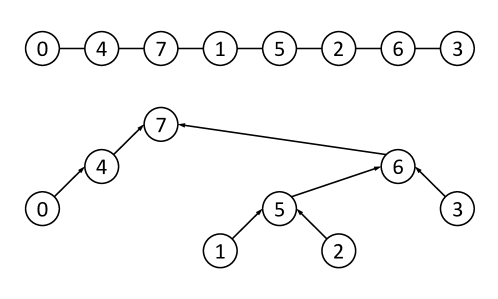
Figure 1: An example of an input list with 8 elements. The number in each element is the priority drawn from a random permutation. The dependences of the contractions are shown as a binary tree structure. In a round-based algorithm [87], the execution is in 4 rounds: $\{0,1,2,3\}$, $\{4,5\}$, then $\{6\}$, and finally $\{7\}$. In Algorithm 1, the execution is asynchronous, and a possible tree-path decomposition is $\{0,4\}$, $\{\varnothing\}$, $\{\varnothing\}$, $\{1\}$, $\{\varnothing\}$, $\{2,5,6,7\}$, $\{\varnothing\}$, and $\{3\}$ for all 8 elements from left to right. The length of a tree-path is bounded by the tree height.

Input: A doubly-linked list $L$ of size $n$. Each element $l_{i}$ has a random priority ($l_{i}.p$), next pointer ($l_{i}.{\mbox{\emph{next}}}$), previous pointer ($l_{i}.{\mbox{\emph{prev}}}$) and flag ($l_{i}.{\mbox{\emph{flag}}}$).

1 parallel foreach element $l_{i}$ in $L$ do

       // set flag if zero or one child

2       $l_{i}.{\mbox{\emph{flag}}}\leftarrow({{\mbox{\emph{pri}}}}(l_{i})<{{\mbox{\emph{pri}}}}(l_{i}.{\mbox{\emph{prev}}}))$ or $({{\mbox{\emph{pri}}}}(l_{i})<{{\mbox{\emph{pri}}}}(l_{i}.{\mbox{\emph{next}}}))$

3parallel foreach element $l_{i}$ in $L$ do

4       $c\leftarrow l_{i}$

       // Execute only if $c$ is a leaf node

5       if ($({{\mbox{\emph{pri}}}}(c)<{{\mbox{\emph{pri}}}}(c.{\mbox{\emph{prev}}}))$ and $({{\mbox{\emph{pri}}}}(c)<{{\mbox{\emph{pri}}}}(c.{\mbox{\emph{next}}}))$)  then

             // Stop when list is contracted into one node

6             while not ($c.{\mbox{\emph{prev}}}$ = null and $c.{\mbox{\emph{next}}}$ = null) do

7                   Splice $c$ out  

8                   Let ${c^{\prime}}$ be $c.{\mbox{\emph{prev}}}$ or $c.{\mbox{\emph{next}}}$ with a smaller priority 

                   // If $c$ is not the last child of $c^{\prime}$, quit

9                   if ${\mbox{\sc{Test-and-Set}}}(c^{\prime}.{\mbox{\emph{flag}}})$ then  break

10                   $c\leftarrow c^{\prime}$ 

11 Function ${{\mbox{\emph{pri}}}}(v)$

12       if $v$ = null then return $\infty$ else return $v.p$

13      

Algorithm 1 ${\mbox{\sc{List-Contraction}}}(L)$

After a more careful investigation, we note that the splicing can proceed asynchronously, and not necessarily based on rounds. For example, the last spliced node with priority 7 separates the list into two disjoint sublists, and the contractions on the two sides are independent and can run asynchronously. Conceptually we can do this recursively, and the recursion depth is $\Theta(\log n)$ whp [87]. Unfortunately, we cannot directly apply the divide-and-conquer approach since $L$ is stored as a linked list and deciding the elements within sublists is as hard as the list contraction algorithm itself.

We present our algorithm in Algorithm 1. Starting from the leaves, Algorithm 1 performs equivalent steps to the algorithm in [87], but its span is $\Theta(\log n)$ in the binary-forking model; this improvement is achieved by allowing the splicing in each round to run asynchronously. The key idea is that, instead of checking all element for readiness in each round, as long as two children of a node $c$ finished contracting, we trigger $c$ to start contracting immediately. The child of $c$ that finished later is responsible for take over $c$, and thus can start immediately. In particular, in the algorithm, a parallel-for loop (Line 1) generates $n$ tasks (threads) each for a node in the list. The loop can be implemented by binary forking for $\log_{2}n$ levels. Only leaf nodes start the execution, and non-leaf nodes quit immediately (Line 1. These leaves will splice themselves out (Line 1), and then try to move upward and splice its parent (Line 1). We note that a node $c$ cannot be contracted until both of its children have been spliced out. Thus we make the child of $c$ that finishes its splicing later to take over $c$. This is achieved by letting the two children compete through Test-and-Set the flag field in $c$ (Line 1). Whichever arrives later takes over and contracts the parent $c^{\prime}$ (Line 1), and the first one simply terminates its computation (Line 1) and let the second one to take continuation. As an example in Figure 1, the threads for nodes 1 and 2 will both try to work on node 5 after they finish their first splicings. They will both attempt to Test-and-Set the flag of node 5. The one coming first succeeds and terminates, and the later one will fail and continue splicing node 5. We initialize the flag for each node to be 0, except for those with 0 or 1 child (Line 1), for which we set flag directly to 1 (they do not need to wait for two children).

Theorem 3.1.

Algorithm 1 for list contraction does $O(n)$ work (worst case) and has $O(\log n)$ span whp in $n$ in the binary-forking model.

Proof.

The correctness of this algorithm can be shown as it applies the same operations as the list contraction algorithm in [87], although Algorithm 1 runs in a much less synchronous manner. The execution of each thread corresponds to a tree-path in the dependence structure starting from a leaf node and ending on either the root or when winning a Test-and-Set. A possible decomposition of the example is shown in the caption of Figure 1. This observation also indicates that the number of iterations of the while-loop on line 1 for any task is $O(\log n)$ whp, bounded by the tree height. The span is therefore $O(\log n)$ whp. The work is linear because every time Line 1–1 is executed, one element will be spliced out. ∎

It is worth noting that, even disregarding the improved 0pt for the binary-forking model, we believe this algorithm is conceptually simpler and easier to implement compared to existing linear-work, logarithmic-time PRAM algorithms [48, 9]. Our algorithm requires starting with a random permutation (discussed further in Section 6). We note that it is straightforward to extend the analysis to using integer priorities instead of random permutations, where the integer priorities are chosen independently and uniformly from the range $[1,n^{k}]$, for $k\geq 2$, with ties broken arbitrarily.

Binary Forking Wyllie.

Here we outline a binary forking version of Wyllie’s algorithm with $O(n\log n)$ work and $O(\log n)$ span, both in the worst case. It is useful for our simulation of logspace in $\mathcal{BF}^{1}$. The idea is to allocate an array of $\log_{2}n$ cells per node of the list, each containing two pointers and a boolean value used for TS. At the end of the algorithm the two pointers in the $i$-th cell (level) will point to the element $2^{i}$ links forward and $2^{i}$ backward in the list (or a null pointer if fewer than $2^{i}$ before or after). The algorithm initially forks off a thread for each node at level 1 in the list. A thread is responsible for splicing out its link at the current level. It does this by writing a pointer to the other neighbor to the corresponding pointer cells of its two neighbors (i.e., splicing itself out), then doing a TS on the boolean flag of each neighbor. For each flag on which it gets a 1 (i.e., it is the second thread to write the pointer at this level), it forks a thread to splice out that neighbor at the next level. Since this fork at the next level only occurs on the second update to the node, both links at the next level must already be available. In general, each splicing step may create 0, 1, or 2 child threads, depending on the timing of arrivals at the neighbors. The first and last element in each list must start with its flag set and writes a null pointer to its one neighbor. As in Wyllie’s original algorithm, it is easy to keep counts to generate the ranks of each node in a list. The total work is proportional to the number of cells, $O(n\log n)$ since each cell gets processed once. Since each fork corresponds to performing a splice at a strictly higher level, the span is proportional to the number of levels, i.e., $O(\log n)$.

4 Sorting

In this section we discuss optimal parallel algorithms to comparison sort and semisort [92] $n$ elements using $O(n\log n)$ and $O(n)$ expected work respectively, and $O(\log n)$ 0pt whp. For comparison sort, the best previous work-efficient result in the binary-forking model requires $O(\log n\log\log n)$ 0pt [45]. In this paper, we discuss a relatively simple algorithm (Algorithm 2) that sorts $n$ elements in $O(n\log n)$ expected work and $O(\log n)$ 0pt whp.

Our algorithm, given in Algorithm 2, is based on sample sorting [59]. It runs recursively. In the base case when the subproblem size falls below a constant threshold, it sorts sequentially. Otherwise, for a subproblem of size $n$, the algorithm selects ${n}^{1/3}\log_{2}n$ samples uniformly at random, and uses the quadratic-work sorting algorithms to sort these samples (i.e., by making all pairwise comparisons). These two steps can be done in $o(n)$ work and $O(\log n)$ 0pt in the binary-forking model. Then the algorithm subselects every $\log_{2}n$-th sample to be a pivot, and use these ${n}^{1/3}$ pivots to partition all elements into ${n}^{1/3}+1$ buckets.

Lemma 4.1.

In the distribution step on Line 2 in Algorithm 2, the number of elements falling into one bucket is no more than $c_{1}rn^{2/3}$ with probability at least $1-n^{-c_{1}}$ for certain constant $r$ and any constant $c_{1}>1$.

This follows from Chernoff bound. The algorithm then allocates ${n}^{1/3}+1$ arrays, one per bucket, each with size $2c_{1}rn^{2/3}$. Then in parallel, each element uses binary search to decide its corresponding bucket. It then tries to add itself to a random position in the bucket by using a TS on a flag to reserve it. If the TS fails, it tries again since the slot is already taken. We limit the number of retries for each element to be no more than $c_{2}\log_{2}n$. If any element cannot find an available slot in this number of retries, the algorithm restarts the process from the random-sampling step (Line 2). Otherwise, after all elements are inserted, the algorithm packs the buckets into contiguous elements for input to the next recursive calls.

1 Let $n=|A|$

2 if $n$ is a constant then  Sort the base case and return

3 Randomly select ${n}^{1/3}\log_{2}n$ samples

4 Use quadratic sorting algorithm to sort the samples

5 Subsample ${n}^{1/3}$ pivots from the samples 

6 Distribute all elements in $A$ to $n^{1/3}+1$ buckets based on the samples (to form a partition of $A$ to $A_{0},A_{1},\ldots,A_{n^{1/3}}$). If failed, restart from Line 2

7 parallel foreach $i\leftarrow 0$ to $n^{1/3}$ do  ${\mbox{\sc{Comparison-Sort}}}(A_{i})$

Algorithm 2 ${\mbox{\sc{Comparison-Sort}}}(A)$

Theorem 4.2.

Algorithm 2 sorts $n$ elements in $O(n\log n)$ expected work and $O(\log n)$ 0pt whp in the binary-forking model.

To bound span, we need to consider the number of retries and the cost of each retry along any path to a leaf in the recursion tree. The number of retries is upper bounded by a geometric distribution since each retry is independent, but the probability of that distribution depends on the level of recursion since problem sizes get smaller. Furthermore the span of a try also depends on the level of recursion (it is bounded by $O(\log n_{i})$, where $n_{i}$ is the input size of level $i$). To help analyze the span, we will use the following Lemma.

Lemma 4.3.

Let $X_{1}\,\cdots,X_{m}$ be independent geometric random variables, and $X_{i}$ has success probability $p_{i}=1-2^{-k^{i}}$ where $k>1$ is a constant. Then $\sum_{i=1}^{m}{k^{i}\cdot X_{i}}\leq O(ck^{m})$ holds with probability at least $1-2^{-ck^{m}}$ for any given constant $c\geq 1$.

Proof.

We view the contribution from each term $k^{i}\cdot X_{i}$ to the sum based on a series of independent unbiased coin flips. The term $k^{i}\cdot X_{i}$ can be considered as the event that we toss $k^{i}$ coins simultaneously, and if all $k^{i}$ coins are heads we charge $k^{i}$ to the sum and this process repeats (corresponding to the geometric random variable with probability $p_{i}=1-2^{-k^{i}}$). However, in this analysis, we toss one coin at a time until we get a tail, and we charge 1 to the sum for each head before the tail. In this way we can only overestimate the sum. Hence, $\sum_{i=1}^{m}{k^{i}\cdot X_{i}}$ can be upper bounded by the number of heads when tossing an unbiased coin until we see $m$ tails. We use Chernoff bound $\Pr(X\leq(1-\delta)\mu)\leq e^{-\delta^{2}\mu/2}$, where $X$ is the sum of indicator random variables, and $\mu=\operatorname{\mathbb{E}}[X]$. Now let’s consider the probability that we see more than $qk^{m}$ heads before $m$ tails. Since $m<k^{m}$, we analyze the probability to see no more than $k^{m}$ tails, which only increases the probability. In this case, we make $(q+1)k^{m}$ tosses, so $\mu=(q+1)k^{m}/2$ and $\delta=(q-1)/(q+1)$. The probability is therefore no more than:

$$\exp\mathopen{}\mathclose{{}\left[-{\mathopen{}\mathclose{{}\left(\frac{q-1}{q+1}}\right)^{2}\cdot\frac{(q+1)k^{m}}{4}}}\right]=\exp\mathopen{}\mathclose{{}\left[-\frac{\mathopen{}\mathclose{{}\left(q-1}\right)^{2}k^{m}}{4(q+1)}}\right]$$

$$= \exp\mathopen{}\mathclose{{}\left[{-\frac{(q^{2}-2q+1)k^{m}}{4(q+1)}}}\right]<\exp\mathopen{}\mathclose{{}\left[{-\frac{(q^{2}-3q-4)k^{m}}{4(q+1)}}}\right]$$

$$= \exp\mathopen{}\mathclose{{}\left[-\frac{(q+1)(q-4)k^{m}}{4(q+1)}}\right]=e^{-\mathopen{}\mathclose{{}\left(\frac{q}{4}-1}\right)k^{m}}<2^{-\mathopen{}\mathclose{{}\left(\frac{q}{4}-1}\right)k^{m}}$$

This proves the lemma by setting $q=4(c+1)$. ∎

Proof of Theorem 4.2.

The main challenge is to analyze the work and 0pt for the distribution cost (Line 2), especially to bound the cost of restarting the distribution step. There are two reasons that the call return to Line 2: badly chosen pivots such that some buckets contain too many elements and become overfull (defined later), or unlucky random number sequences such that the positions tried by a particular element are all occupied (for more than $c_{2}\log n$ consecutive slots). We say a bucket is overfull if it has more than $c_{1}rn^{2/3}$ elements (more than half of the allocated space). From Lemma 4.1, the probability of this event is no more than $n^{-c_{1}}$. We pessimistically assume that the distribution step restarts once a bucket is overfull. Therefore, for the latter case with a bad random number sequence, the allocated array is always no more than half-full, which is useful in analyzing this case.

We now analyze the additional costs for the restarts. For the latter case, with probability at most $n^{1-c_{2}}$, at least one element retries more than $c_{2}\log_{2}n$ times. For the first case, the probability that any bucket is oversize is $n^{1-c_{1}}$. By setting $c_{1}$ and $c_{2}$ to be at least 2, the expected work including restarts is asymptotically bounded by the first round of selecting pivots and distributing the elements. The work of the first round is bounded by $O(n\log n)$ since there are $n$ elements, each doing a binary search and then each trying at most $O(\log n)$ locations. Therefore the expected work for each distribution is $O(n_{i}\log n_{i})$, where $n_{i}$ is the size of the input.

The total number of elements across any level of recursion is at most $n$ since every element goes to at most one bucket. Also the size of each input reduces to at most $kn^{2/3}$ from level to level, for some constant $k$. The total expected work across each level of recursion therefore decreases geometrically from level to level. Hence the total work is asymptotically bounded by the work at the root of the recursion, which is $O(n\log n)$ in expectation.

We now focus on the 0pt, and first analyze the case for the chain of subproblems for one element. The number of recursive levels is $O(\log\log n)$. For each level with subproblem size $n^{\prime}$, let $c=c_{1}=c_{2}\geq 2$. The probability for a restart is less than $2(n^{\prime})^{1-c}$, and the 0pt cost for a restart is $c\log_{2}n$. Treating the number of restarts in each level as a random variable, we can plug in Lemma 4.3 with $k=1.5$ and $m=\log_{1.5}\log_{2}n$, and show that the 0pt of this chain is $O(ck^{m})=O(c\log n)$ with probability at least $1-2^{-c\log n}=1-n^{-c}$. Then by taking a union bound for the $n$ chains to all leaves of the recursion, the probability is at least $1-n^{1-c}$. Combining the analyses of the work and the 0pt proves the theorem. ∎

Semisorting. Semisorting reorders an input array of $n$ keys such that equal keys are contiguous but different keys are not necessarily in sorted order. It can be used to implement integer sort with a small key range. Semisorting is a widely-used primitive in parallel algorithms (e.g., the random permutation algorithm in Section 6).

We note that with the new comparison sorting algorithm with optimal work and 0pt, we can plug it in the semisorting algorithm by Gu et al. [65] (Step 3 in Algorithm 1). The rest of the algorithm is similar to the distribution step but just run for one round, so it naturally fits in the binary-forking model with no additional cost. Hence, this randomized algorithm is optimal in the binary-forking model—$O(n)$ expected work and $O(\log n)$ 0pt whp.

5 Ordered Set-set Operations

In this section, we show deterministic algorithms for ordered set-set operations (Union, Intersection and Difference) based on weight-balanced binary search trees. In particular we prove the following theorem.

Theorem 5.1.

Union, Intersection and Difference of two ordered sets of size $n$ and $m<n$ can be solved in $O\mathopen{}\mathclose{{}\left(m\log\mathopen{}\mathclose{{}\left(\frac{n}{m}+1}\right)}\right)$ work and $O(\log n)$ span in the binary-forking model. This is optimal for comparison-based algorithms.

Our approach is based on a (roughly $\sqrt{n}$-way) divide-and-conquer algorithm with lazy reconstruction-based rebalancing. At a high-level, for two sets of size $n$ and $m\,(\leq n)$, we will split both trees with $d-1$ pivots equally distributed among the $m+n$ elements, where $d=\Theta(\sqrt{m+n})$ is a power of 2. The algorithm runs recursively until the base case when $m^{\prime}\leq\sqrt{m^{\prime}+n^{\prime}}$, where $m^{\prime}$ and $n^{\prime}$ are the sizes of the two input trees in the current recursive call, respectively. For the base cases, we apply a weaker (work-inefficient) algorithm discussed in Appendix A. The work-inefficient approach will not affect the overall asymptotic bound because of the criterion at which the base cases are reached. After that, the $d$ pieces are connected using the pivots. At this time, rebalancing may occur, but we do not handle it immediately. Instead, we apply a final step at the end of the algorithm to recursively rebalance the output tree based on a reconstruction-based algorithm discussed in Section 5.4. The high-level idea is that, whenever a subtree has two children imbalanced by more than some constant factor (i.e., one subtree is much larger than the other one), the whole subtree gets flattened and reconstructed. Otherwise, the subtree can be rebalanced using a constant number of rotations. An illustration of our algorithm is shown in Figure 2. Due to page limitation, we put the algorithm description of base case algorithms (Appendix A), and the cost analysis of the algorithm (Appendix B) in the appendix, and only briefly show some intuition in Section 5.5.

5.1 Background and Related Work

Ordered set-set operations Union, Intersection and Difference are fundamental algorithmic primitives, and there is a rich literature of efficient algorithms to implement them. For two ordered sets of size $n$ and $m\leq n$, the lower bound on the number of comparisons (and hence work or sequential time) is $\Omega\mathopen{}\mathclose{{}\left(m\log\mathopen{}\mathclose{{}\left(\frac{n}{m}+1}\right)}\right)$ [70]. The lower bound on span in the binary-forking model is $\Omega(\log n)$. Many sequential and parallel algorithms match the work bound [30, 21, 5, 37]. In the parallel setting, some algorithms achieve $O(\log n)$ span on the PRAM [81, 80]. However, they are not work-efficient, requiring $O(m\log n)$ work. There is also previous work focusing on I/O efficiency [15] and concurrent operations [57, 36] for parallel trees, and parallel data structures supporting batches [64, 4, 78].

Some previous algorithms achieve optimal work and polylogarithmic span. Blelloch and Reid-Miller proposed algorithms on treaps with optimal expected work and $O(\log n)$ span whp on an EREW PRAM with scan operations, which translates to $O(\log^{2}n)$ span in the binary-forking model. Akhremtsev and Sanders [5] described an algorithm for array-tree Union based on $(a,b)$-trees with optimal work and $O(\log n)$ span on a CRCW PRAM. Blelloch et al. [30] proposed ordered set algorithms for a variety of balancing schemes [21] with optimal work. All the above-mentioned algorithms have $O(\log m\log n)$ span in the binary-forking model. There have also been parallel bulk operations for self-adjusting data structures [4]. As far as we know, there is no parallel algorithm for ordered set functions (Union, Intersection and Difference) with optimal work and $O(\log n)$ span in the binary-forking model.

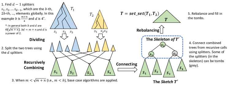
Figure 2: An illustration of the set-set algorithms. We first split both trees into chunks by the glaobally $b$-th, $2b$-th, …, elements. Here $b=\frac{m+n}{4}$, but in general $b=(n+m)/d$ should be $\Theta(\sqrt{m+n})$ where $d=\Theta(\sqrt{m+n})$ is a power of 2. We then recursively sketch each pair of chunks, until we reach the base case and call the base case algorithms. We then connect the results with pivots, and get the sketch of the result tree. Finally we rebalance the tree structure and fill in all tombs.

5.2 Preliminaries

Given a totally ordered universe $U$, the problem is to take the union, intersection, and difference of two subsets of $U$. We assume the comparison model over the elements of $U$, and require that the inputs and outputs can be enumerated in-order with no additional comparison (i.e., no cheating by being lazy).

We assume the two inputs have sizes $m$ and $n\geq m$ stored in weight-balanced binary trees [79] with balancing parameter $\alpha$ (WBB[$\alpha$] tree). The weight of a subtree is defined as its size plus one, such that the weight of a tree node is always the sum of the weights of its two children. WBB[$\alpha$] trees maintain the invariant that for any two subtrees of a node, the weights are within a factor of $\alpha$ ($0<\alpha\leq 1-1/\sqrt{2}$) of each other. For the two input trees, we refer to the tree of size $n$ as the large tree, denoted as $T_{L}$, and the tree of size $m$ as the smaller tree, denoted as $T_{S}$. We present two definitions as follows. Note that these two definitions are more general than the definitions of ancestors and descendants, since $k$ may or may not appear in $T$.

Definition 1.

In a tree $T$, the upper nodes of an element $k\in U$, are all the nodes in $T$ on the search path to $k$ (inclusive).

Definition 2.

In a tree $T$, an element $k\in U$ falls into a subtree $T_{x}\in T$, if the search path to $k$ in $T$ overlaps the subtree $T_{x}$.

Persistent Data Structures.

In this section, we use underlying persistent [55] (and actually purely functional) tree structure, which uses path-copying to update the weight-balanced trees. This means that when a change is made to a node $v$ in the tree, a copy of the path to $v$ is made, leaving the old path and old value of $v$ intact. Figure 3 shows an example of inserting a new element into the tree. Such a persistent insertion algorithm also copies nodes that are involved in rotations since their child pointers change.

In particular, our algorithm will use a persistent Split$(T,k)$ function on WBB$[\alpha]$ trees as discussed in [21, 88]. This function splits tree $T$ by key $k$ into two trees and a bit, such that all keys smaller than $k$ and larger than $k$ will be stored the two output trees, respectively, and the bit indicates if $k\in T$. Because of path-copying, the persistent Split returns two output trees and leaves the input tree intact. This algorithm costs $O(\log n)$ work on a tree of size $n$.

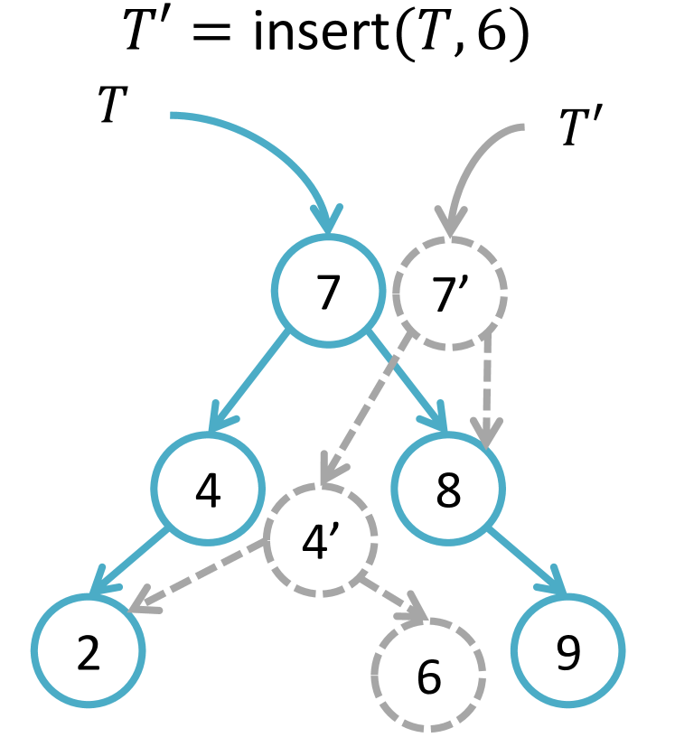
Figure 3: A persistent insertion on a tree. The algorithm basically copies all tree nodes on the insertion path, such that the new (copied) root represents the output tree, and the input tree is intact represented by the old root pointer. This algorithm costs $O(\log n)$ time for an input tree of size $n$.

Input: Two weight-balanced trees storing two ordered sets.

Output: A weight-balanced tree $T$ storing the union/intersection/difference of the two input sets.

1 if $|T_{1}|<|T_{2}|$ then return Set_Set$(T_{2},T_{1})$

2 $T^{\prime}\leftarrow{\mbox{\sc{Sketch}}}(T_{1},T_{2})$ // Algorithm 4

3 $T\leftarrow{\mbox{\sc{Rebalance}}}(T^{\prime},{\mbox{\sc{false}}})$ // Algorithm 5

return $T$

Algorithm 3 $T\leftarrow{\mbox{\sc{Set\_Set}}}(T_{1},T_{2})$, the main algorithm for ordered set-set operations

Input: Two WBB$[\alpha]$ trees. $T_{1}$ is from the original larger tree $T_{L}$ and $T_{2}$ is from the original smaller tree $T_{S}$.

Output: A binary tree sketch $T^{\prime}$ representing the union/intersection/difference of the two input sets.

1 Let $n^{\prime}\leftarrow|T_{1}|$ and $m^{\prime}\leftarrow|T_{2}|$

2 if $n^{\prime}$ is $0$ then  return $T_{2}$

3 if $m^{\prime}$ is $0$ then  return $T_{1}$

4 if $m^{\prime}<\sqrt{n^{\prime}+m^{\prime}}$ then  return ${\mbox{\sc{Base\_Case}}}(T_{1},T_{2})$

5 $d\leftarrow 2^{\lceil\log_{2}\sqrt{m^{\prime}+n^{\prime}}\rceil}$

6 $b\leftarrow(m^{\prime}+n^{\prime})/d$

7 Let ${\mbox{\emph{splitter}}}_{0}\leftarrow-\infty$ and ${\mbox{\emph{splitter}}}_{d}\leftarrow+\infty$

8 parallel for $i\leftarrow 1$ to $d-1$ do

9       Find ${\mbox{\emph{splitter}}}_{i}$, which is the $(i\cdot b)$-th element in $T_{1}$ and $T_{2}$ (duplicate value counts twice) by dual-binary search

10       Let $f_{i}$ indicate if ${\mbox{\emph{splitter}}}_{i}$ is a tomb

11      

12parallel for $i\leftarrow 1$ to $d$ do

13       Split $T_{1}$ using ${\mbox{\emph{splitter}}}_{i-1}$ and ${\mbox{\emph{splitter}}}_{i}$, output tree $T_{1,i}$

14       Split $T_{2}$ using ${\mbox{\emph{splitter}}}_{i-1}$ and ${\mbox{\emph{splitter}}}_{i}$, output tree $T_{2,i}$

15       $T^{\prime}_{i}\leftarrow{\mbox{\sc{Sketch}}}(T_{1,i},T_{2,i})$

16Connect $T^{\prime}_{1},\ldots,T^{\prime}_{d}$ using ${\mbox{\emph{splitter}}}_{1},\ldots,{\mbox{\emph{splitter}}}_{d-1}$

17 return the result tree

Algorithm 4 $T^{\prime}\leftarrow{\mbox{\sc{Sketch}}}(T_{1},T_{2})$

Input: A tree sketch $T^{\prime}$, and a boolean flag last indicating if the last element should be extracted.

Output: A valid weight-balanced tree $T$ with no tombs. If last is true, $e$ is the last element extracted from $T^{\prime}$.

Note : ${\mbox{\sc{EffectiveSize}}}(T)$ returns the number of non-tombs in $T$.

1 if ${\mbox{\sc{EffectiveSize}}}(T^{\prime})$ is $0$ then return $\langle\varnothing,\varnothing\rangle$

2 if $T^{\prime}$ is obtained by base cases (Line 4 in Algorithm 4 then

3       if last then return $\langle{\mbox{\sc{RemoveLast}}}(T^{\prime}),{\mbox{\sc{Last}}}(T^{\prime})\rangle$

4       else return $\langle T^{\prime},\varnothing\rangle$

5      

6if no nodes in $T_{S}$ fall into $T^{\prime}$ (by checking small$(T^{\prime})$) then

7       if last then return $\langle{\mbox{\sc{RemoveLast}}}(T^{\prime}),{\mbox{\sc{Last}}}(T^{\prime})\rangle$

8       else return $\langle T^{\prime},\varnothing\rangle$

9      

10if last then $b\leftarrow 1$ else $b\leftarrow 0$

11 if ${\mbox{\sc{EffectiveSize}}}({\mbox{\sc{LeftTree}}}(T^{\prime}))+1$ and ${\mbox{\sc{EffectiveSize}}}({\mbox{\sc{RightTree}}}(T^{\prime}))-b+1$ differs by more than a factor of $2/\alpha$ then

12       Flatten $T^{\prime}$ and reconstruct it (if last then extract the last element in $T^{\prime}$) 

13       return the new tree

14if the root of $T^{\prime}$ is a tomb then $t\leftarrow\texttt{true}$ else $t\leftarrow\texttt{false}$

15 In parallel: 

16       $\langle T_{l},e_{l}\rangle={\mbox{\sc{Rebalance}}}({\mbox{\sc{LeftTree}}}(T^{\prime}),t)$

17       $\langle T_{r},e_{r}\rangle={\mbox{\sc{Rebalance}}}({\mbox{\sc{RightTree}}}(T^{\prime}),{\mbox{\emph{last}}})$

18      

19if ${\mbox{\sc{EffectiveSize}}}({\mbox{\sc{RightTree}}}(T^{\prime}))$ is 0 and last then

20       $T\leftarrow T_{l}$

21       if the root of $T^{\prime}$ is a tomb then $e\leftarrow e_{l}$

22       else $e\leftarrow T^{\prime}.{\mbox{\emph{root}}}$

23      

24else

25       $e\leftarrow e_{r}$

26       if the root of $T^{\prime}$ is a tomb then $T\leftarrow{\mbox{\sc{Connect}}}(T_{l},e_{l},T_{r})$

27       else $T\leftarrow{\mbox{\sc{Connect}}}(T_{l},T^{\prime}.{\mbox{\emph{root}}},T_{r})$

28      

return $\langle{\mbox{\sc{RebalanceByRoatation}}}(T),e\rangle$

Algorithm 5 $\langle T,e\rangle\leftarrow{\mbox{\sc{Rebalance}}}(T^{\prime},{\mbox{\emph{last}}})$

5.3 The Main Algorithms

We first give a high-level description of our algorithms for the three set-set functions. As mentioned, we denote the larger input tree as $T_{L}$, and the smaller input tree as $T_{S}$. We use two steps, sketching and rebalancing. The sketching step aims at combining the elements in the two input trees in-order into one tree, which is not necessarily balanced. The rebalancing step will apply a top-down algorithm to rebalance the whole tree by the WBB[$\alpha$] criteria.

Our sketching algorithm is based on a $d$-way divide-and-conquer scheme, where $d=\Theta(\sqrt{n+m})$ is a power of 2. It is a recursive algorithm, for which the two input trees are denoted as $T_{1}$ and $T_{2}$. In particular, $T_{1}$ contains a subset of $T_{L}$ and $T_{2}$ contains a subset of $T_{S}$. The algorithm will combine the two subsets and return one result tree. Note that even though $T_{1}\subseteq T_{L}$ and $T_{2}\subseteq T_{S}$, the sizes of $T_{1}$ is not necessarily larger than $T_{2}$. Throughout the recursive process, we track the following quantities for each tree node $v$:

1. The size of the subtree, noted as $\text{size}(v)$.

2. The number of elements originally from $T_{L}$, noted as $\text{large}(v)$.

3. The number of elements originally from $T_{S}$, noted as $\text{small}(v)$.

4. The number of elements appearing both in $T_{L}$ and $T_{S}$, noted as $\text{common}(v)$.

The tree size $\text{size}(v)$ is required by the WBB[$\alpha$] invariant. The other three are used for $T_{L}-T_{S}$, $T_{S}-T_{L}$, and $T_{S}\cap T_{L}$ respectively. The generic algorithm for all three operations is given in Algorithms 3, 4, and 5. An illustration is shown in Figure 2. The difference between the three set-set functions is only in the base cases.

We now present the two steps of the algorithm in details:

1. Sketching (Algorithm 4). This step generates an output tree $T^{\prime}$ with all elements in the result, although not rebalanced. There are three subcomponents in this step. Denote $n^{\prime}=|T_{1}|$ and $m^{\prime}=|T_{2}|$, which means the number of tree nodes handled by this recursive call that are originally from the larger and smaller tree, respectively. As mentioned, $m^{\prime}$ can be even larger than $n^{\prime}$ in some of the recursive calls.

   1. Base Case. When $m^{\prime}<\sqrt{n^{\prime}+m^{\prime}}$, the algorithm reaches the base case. It calls the work-inefficient algorithm to generate a balanced output tree in $O(m^{\prime}\log n^{\prime})$ work and $O(\log n^{\prime})$ span, which are presented in Appendix A.

   2. Dividing. We then use $d-1$ pivots to split both input trees into $d$ chunks, and denote the partitioning of $T_{1}$ as $T_{1,\{1,\ldots,d\}}$, and $T_{2}$ as $T_{2,\{1,\ldots,d\}}$. The $d-1$ pivots are the global $b$-th, $2b$-th, …elements in the two trees, where $b=(n+m)/d$, so that $|T_{1,i}|+|T_{2,i}|$ for all $i$ have the same value (or differ by at most 1). All the splits (Line 4) can be done in parallel using a persistent split algorithm on weight-balanced trees [21]. We then apply the algorithm recursively on each pair of chunks.

      Note that not all the pivots should appear in the output tree of the entire algorithm, depending on the set function. For example, for Intersection, those pivots that only appear in one tree will not show up at the end. In this case, in the Sketch step, we will mark such pivot nodes as tombs, and filter them out later in the rebalancing step.

   3. Connecting. After the dividing substep and recursive calls, we have $d-1$ pivots (including tombs), and $d$ combined chunks returned by the recursive calls. In the connecting substep, we directly connect them regardless of balance. Since $d$ is a power of 2, the $d-1$ pivots will form a full balanced binary tree structure on the top $\log_{2}d$ levels, and all the chunks output from recursive calls will dangle on the $d$ pivots. This process is shown in Line 4.

   The output $T^{\prime}$ of the Sketch step is a binary tree, which may or may not be balanced. We will call $T^{\prime}$ the sketch of the final output of the algorithm. We also call the top $\log_{2}d$ levels in $T^{\prime}$ consists of pivots the skeleton of $T^{\prime}$. We note that $T^{\prime}$ may contain tombs, and we will filter them out in the next step.

2. Rebalancing. We will use a reconstruction-based rebalancing algorithm to remove the tombs and rebalance the sketch tree $T^{\prime}$ (Algorithm 5, see more details in Section 5.4). This rebalancing algorithm is stand-alone, and is of independent interest.

5.4 The Rebalancing Algorithm

We now present the reconstruction-based rebalancing algorithm. A similar idea was also used in [28]. In this paper, we use this technique to support better parallelism instead of write-efficiency.

We use the effective size of a subtree as the number of elements in this subtree excluding all tombs. The effective size for a tree node $v$ can be computed based on size($v$), large($v$), small($v$) and common($v$), depending on the specific set operation. It is used to determine if two subtrees will be balanced after removing all tombs.

The rebalancing algorithm is given in Algorithm 5. The algorithm recursively settles each level top-down. For a tree node, we check the effective sizes of its two children and decide if they are almost-balanced. Here almost-balanced indicates that sizes of the two subtrees differ by at most a factor of $2/\alpha$. If not, we flatten the subtree and re-build it. Otherwise, we recursively settle its two children, and after that we re-connect the two subtrees back and rebalance using at most a constant number of rotations.

We also need to filter out tombs, since they should not appear in the output tree. We do this recursively. If the current subtree root of $T^{\prime}$ in Algorithm 5 is a tomb, we will need to fill it in using the last element in its left subtree. We note that the effective size of the left subtree cannot be 0 (otherwise the algorithm returns at Line 5). To do this, the algorithm will take an extra boolean argument last denoting if the last element of the result needs to be extracted (returned as $e$ in the output of Algorithm 5). In this case, if the root of $T^{\prime}$ is a tomb, the algorithm simply passes a true value to the left recursive call, getting the last element to replace the tomb.

For computing the last value (denoted as $r$), there are two cases. First, if the subtree needs rebalancing, then after flattening the elements into an array, we simply take out the last element in the array as $r$ and return. Extracting the last element is inlined in the process of reconstruction (Line 5). Otherwise, we recursively deal with the two subtrees. If last is true, we also extract the last element in its right subtree.

Multiple base cases apply to this rebalancing algorithm. If the effective size of $T^{\prime}$ is 0, the algorithm directly returns an empty tree and an empty element. The second case is when no element in $T_{S}$ falls into $T^{\prime}$. This can be determined by looking at ${\mbox{\emph{small}}}(T^{\prime})$. Note that all the chunks in the sketching algorithm is designed to be the same size. Therefore, in this case, the whole subtree should be (almost) perfectly balanced, so we directly return it. These base cases are essential in bounding the work of rebalancing, since we do not need to traverse the whole subtree for these special cases.

5.5 Base Case Algorithms and Cost Proof Outline

Due to page limitation, we put the algorithm description of base case algorithms and the cost analysis of the algorithm in the appendix. Here we show a very brief description about the intuition.

Base case algorithms. The base case algorithms ${\mbox{\sc{Base\_Case}}}(T_{1},T_{2})$ in Algorithm 4 use an work-inefficient version ($O(m^{\prime}\log n^{\prime})$ work and $O(\log(n^{\prime}+m^{\prime}))$ span) of the set-set algorithms. These algorithms are applied when $m^{\prime}<\sqrt{n^{\prime}+m^{\prime}}$, which guarantees the total base case cost is $O\mathopen{}\mathclose{{}\left(m\log\mathopen{}\mathclose{{}\left(\frac{n}{m}+1}\right)}\right)$. The intuition of the base case algorithms is to search all $m^{\prime}$ elements from $T_{1}$ in $T_{2}$, and based on the set operation being performed, add (remove) the $m^{\prime}$ elements into (from) $T_{2}$. The same rebalancing algorithm as in Section 5.4 is applied to guarantee a balanced output tree. Detailed description is in Appendix A.

Span. We will show that all base cases, Sketch, and Rebalance algorithms have span $O(\log(n+m))$. We first prove that the height of the sketch $T^{\prime}$ is $O(\log(n+m))$ (Lemma B.5). The span of the base cases is straight-forward. For Sketch, this bound holds because of the $\sqrt{m+n}$-way divide-and-conquer. For Rebalance, the span holds because the algorithm settles each node top-down, and settling each level in the skeleton only costs a constant span. For the skeleton of the returned tree, if a node is nearly-balanced, then a constant number of rotations settles it. Otherwise, flattening and reconstructing a tree of height $h$ takes $O(h)$ span, which is also equivalent to a constant per level. In all, the span is $O(\log(n+m))$. We formally prove the span of the algorithm in Lemma B.6.

Work bound. For work, we will prove that all base cases, Sketch, and Rebalance algorithms cost work $O\mathopen{}\mathclose{{}\left(m\log\mathopen{}\mathclose{{}\left(\frac{n}{m}+1}\right)}\right)$. We first show that the number of pivots is $O(m)$ (Lemma B.4). Most interestingly, for Rebalance, the optimality in work lies in the reconstruction-based algorithm. For all pivots in the skeleton, if it is nearly balanced, the rebalancing cost is a constant. Therefore the total work is proportional to the size of the skeleton, which is no more than $O\mathopen{}\mathclose{{}\left(m\log\mathopen{}\mathclose{{}\left(\frac{n}{m}+1}\right)}\right)$.

To show the total reconstruction work, in the sketch $T^{\prime}$, we mark all upper nodes of the elements in $T_{S}$ as red. There are at most $O\mathopen{}\mathclose{{}\left(m\log\mathopen{}\mathclose{{}\left(\frac{n}{m}+1}\right)}\right)$ red nodes in $T^{\prime}$ (Lemma B.1). We will show that the reconstruction work averaged to each red node is a constant. The key observation is that, rebalancing for a subtree $T_{x}\in T^{\prime}$ happens only when there are $m_{x}\geq c|T_{x}|$ red nodes in $T_{x}$, where $c$ is a constant. This is because the two subtrees of $T_{x}$ are supposed to have the same size ($\sqrt{n^{\prime}+m^{\prime}}$) due to the selection of pivots. However there can be duplicates in Union; also Intersection and Difference do not keep all input elements in the output. Therefore there can be imbalanced in size. We will show that the size of either subtree changes by no more than $m_{x}$. Therefore, to make them unbalanced, $m_{x}$ has to be at least $c|T_{x}|$ for some constant $c$. This makes the average cost per red node to be $O(1)$. Adding the cost of all red nodes gives the stated optimal work bound. We will formally prove the work of the algorithm in Lemma B.10.

6 Random Permutation

Generating random permutation in parallel is useful in parallel algorithms, and is used in the list and tree contraction algorithms in this paper. Hence it has been well-studied both theoretically [6, 8, 51, 61, 62, 63, 66, 68, 77, 82, 87] and experimentally [49, 67, 87]. To the best of our knowledge, none of these algorithms can be implemented in the binary-forking model using linear work and $O(\log n)$ 0pt. We now consider the simple sequential algorithm of Knuth [76] (Durstenfeld’s [56]) shuffle that iteratively decides each element:

1 Function KnuthShuffle(A, H)

2       $A[i]\leftarrow i$ for all $i=0,\ldots,n-1$

3       for $i\leftarrow n-1$ to $0$ do

4             swap($A[i]$, $A[H[i]]$)

where $H[i]$ is an integer uniformly drawn between 0 and $i-1$, and $A[\cdot]$ is the output random permutation.

A recent paper [87] shows that this sequential iterative algorithm is readily parallel. The key idea is to apply multiple swaps in parallel as long as the sets of source and destination locations of the swaps are disjoint. Figure 4 shows an example, and we can swap location 5 and 2, 7 and 1, 6 and 3 simultaneously in the first round, and the three swaps do not interfere each other. If the nodes pointing to the same node are chained together and the self-loops are removed, we get the dependences of the computation. An example is given in Figure 4(b). Similar to list contraction, we can execute the swaps for all leaf nodes and remove them from the tree in a round-based manner. It can be shown that the modified dependences by chaining all the roots in the dependence forest (as shown in Figure 4(c)) correspond to a random binary search tree, and the tree depth is again bounded by $O(\log n)$ whp. The 0pt of this algorithm is therefore $O(\log^{2}n)$ whp in the binary-forking model.

Similar to the new list contraction algorithm discussed in Section 3, the computation can be executed asynchronously. Namely, the swaps in different leaves or subtrees are independent. Therefore, once the dependence structure is generated, we can apply a similar approach as in Algorithm 1, but instead of splicing out each node, we swap the values for the pair of nodes.

The remaining question is how to generate the dependence structure. We do this in two steps. We first semisort all nodes based on the destination locations (grouping the nodes on all the horizontal chains in Figure 4(b) or right chains in Figure 4(c)). Then we use an algorithm that takes quadratic work to sort the nodes within each group, and connect the nodes as discussed.

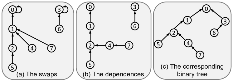
Figure 4: An example when $H=[0,0,1,3,1,2,3,1]$. Figure (a) indicates the destinations of the swaps shown by $H$. The dependences of the swaps are shown by Figure (b), indicating the order of the swaps. Figure (c) links the roots of the forest to make it a binary tree.

Theorem 6.1.

The above algorithm generates a random permutation of size $n$ using $O(n)$ expected work and $O(\log n)$ span whp in the binary-forking model.

Proof.

Similar to the list contraction algorithm in Section 3, this algorithm applies the same operations as the random permutation algorithm in [87], and the swaps obey the same ordering for any pair of nodes with dependency. The improvement for 0pt is due to allowing asynchrony for disjoint subtrees.

The cost after the construction of dependence tree is the same as the list contraction algorithm (Algorithm 1), which is $O(n)$ work and $O(\log n)$ span whp. For constructing the dependence tree, the semisort step takes $O(n)$ expected work and $O(\log n)$ 0pt whp using the algorithm in Section 4. The quadratic work sorting can easily be implemented in $O(\log n)$ 0pt whp, as in Section 4. We now analyze the work to sort the chains.

Let a 0/1 random variable $A_{i,j}$ is 1 if $H[i]=j$ for $j<i$, and the probability $\Pr[A_{i,j}=1]$ is $1/i$. $\Pr[A_{i,j}A_{k,j}=1]$ is then $1/(ik)$ for $j<i<k$ since they are independent. The expected overall work for sorting is (omitting constant in front of $A_{i,j}$).

$$\operatorname{\mathbb{E}}[W_{{\scriptsize\mbox{\emph{RandPerm}}}}(n)]=\operatorname{\mathbb{E}}\mathopen{}\mathclose{{}\left[\sum_{j=1}^{n}\mathopen{}\mathclose{{}\left(\sum_{i=j}^{n}{A_{i,j}}}\right)^{2}}\right]$$

$$= \operatorname{\mathbb{E}}\mathopen{}\mathclose{{}\left[\sum_{j=1}^{n}\sum_{i=j}^{n}{A_{i,j}^{2}}}\right]+2\cdot\operatorname{\mathbb{E}}\mathopen{}\mathclose{{}\left[\sum_{j=1}^{n}\sum_{i=j+1}^{n}\sum_{k=i+1}^{n}{A_{i,j}A_{k,j}}}\right]$$

$$= \sum_{i=1}^{n}\sum_{j=1}^{i-1}{1/i}+\sum_{k=1}^{n}\sum_{i=1}^{k-1}\sum_{j=1}^{i-1}{1/ik}~{}=~{}O(n)$$

Combining all results gives the stated theorem. ∎

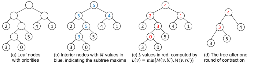
Figure 5: An example of the tree contraction algorithm. It first generates the priority of the leaf node from a random permutation, as shown in Figure (a). Then every interior node computes the highest priority label in the subtree, and the computed values are shown as the blue numbers in Figure (b). Then each interior node $v$ is paired with the leaf node that has the priority which is stored in the child node different from the priority of $v$. Taking the root node as an example, the priority 5 is different from the right node which has priority 4, so the root node is paired with the leaf node with priority 4. The pairing results are shown as the red numbers in Figure (c). In this example, leaf nodes 0, 1, and 2 can be contracted simultaneously, and the contracted tree is shown in Figure (d).

7 Range Minimum Queries

Given an array $A$ of size $n$, the range minimum query (RMQ) takes two input indices $i$ and $j$, and reports the minimal value within this range. RMQ is a fundamental algorithmic building block that is used to solve other problems such as the lowest common ancestor (LCA) problem on rooted trees, the longest common prefix (LCP) problem, and lots of other problems on trees, strings and graphs.

An optimal RMQ algorithm requires linear preprocessing work and space, and constant query time. It can be achieved by a variety of algorithms (e.g., [17, 16, 7, 58, 10]). These algorithms are based on the data structure referred to as the sparse table that can be precomputed in $O(n\log n)$ work where $n$ is the input size, and constant RMQ cost. To further improve the work, the high-level idea in these algorithms is to chunk the array into $O(n/\log n)$ groups each with size $O(\log n)$, find the minima of the groups, and only preprocess the sparse table for the minima. Within each group, these algorithms use different techniques to preprocess in $O(\log n)$ work per group, and support constant query cost within each group. Then for a range minimum query $(i,j)$, the minimum can be answered by combining by the query for the sparse table for the whole groups in this range, and the query for the boundary groups that contain elements indexed at $i$ and $j$. These algorithms can be trivially parallelized in the PRAM model using $O(\log n)$ span (time), but when translating to the binary-forking model, the span becomes $O(\log^{2}n)$ in preprocessing the sparse table, and needs to be improved.

For simplicity, we first assume the number of groups $n^{\prime}$ is a power of 2. In the classic sparse table, we denote $T_{i,k}$ as the minimal value between group range $i$ and $i+2^{k}-1$. It can be computed as $\min\mathopen{}\mathclose{{}\left\{T_{i,k-1},T_{i+2^{k-1},k-1}}\right\}$. Let $k=\lfloor\log_{2}{(j-i)}\rfloor$. Then for query from group $i$ to $j(>i)$, we have ${\mbox{\emph{RMQ}}}(i,j)=\min\mathopen{}\mathclose{{}\left\{T_{i,k},T_{j-2^{k}+1,k}}\right\}$. Directly parallelizing the construction for the sparse table uses $O(\log^{2}n)$ 0pt—$O(\log n)$ levels in total and $O(\log n)$ 0pt within each level. We now consider a variant of the sparse table which is easier to be generated in the binary-forking model and equivalently effective.

In the modified version, we similarly have $\log_{2}n^{\prime}$ levels, and in $k$-th level we partition the array into $n^{\prime}/2^{k}$ subarrays each with size $2^{k}$. For each subarray, we further partition it to two parts with equal size, and compute the suffix minima for the left side, and prefix minima for the right side. We denote $T^{\prime}_{i,k}$ as such value with index $i$ in the $k$-th level. For each query $(i,j)$, we find the highest significant bit that is different for $i$ and $j\geq i$. If this bit is the $k$-th bit from the right, then we have ${\mbox{\emph{RMQ}}}(i,j)=\min\mathopen{}\mathclose{{}\left\{T^{\prime}_{i,k},T^{\prime}_{j,k}}\right\}$. An illustration is shown in Figure 6.

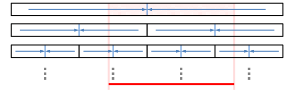
Figure 6: An illustration of the modified sparse table in Section 7. The range is hierarchically partitioned into logarithmic number of levels, and the prefix and suffix minima are computed as the arrows indicate. For each query range shown as the red segment, we can locate a unique level such that the minimum of the range can be answered by the suffix and the prefix minima (the shaded range).

We now describe how to compute $T^{\prime}_{i,k}$. We note that the computation for each subarray is independent, and each takes linear work and logarithmic 0pt proportional to the subarray size [18]. Since each element corresponds to $\log_{2}n^{\prime}$ computed values, the overall cost is therefore $O(n^{\prime}\cdot\log_{2}n^{\prime})=O(n)$ work and $O(\log n)$ 0pt.

Theorem 7.1.

The range minimum queries for an array of size $n$ can be preprocessed in $O(n)$ work and $O(\log n)$ 0pt in the binary-forking model, and each query requires constant cost.

8 Tree Contraction

Parallel algorithms for tree contraction have received considerable interest because of its ample applications for many tree and graph applications [73, 77, 85, 87, 13]. There are many variants of parallel tree contraction. Here we will assume we are contracting rooted binary trees in which every internal node has exactly two children. Any rooted tree can be reformatted to this shape in linear work and logarithmic span. We assume the tree $T$ has $n$ leaf nodes (and $n-1$ interior nodes). We use $v.lC$ and $v.rC$ to denote the left and the right child of a node $v$, respectively.

List contraction can be considered as a degenerated case of tree contraction when all interior nodes are chained up. As a result, we do not know an optimal parallel algorithm for tree contraction with $O(n)$ work and $O(\log n)$ span. Similarly, the difficulty in designing such an algorithm remains in using no synchronization.

Here we consider parallelizing the sequential iterative algorithm that “rakes” one leaf node at a time. A rake operation removes a leaf node and its parent node $v$, and if $v$ is not the root, it sets the other child of $v$ to replace $v$ as the child of $v$’s parent. We assign each leaf node a priority drawn from a random permutation, so the priority defines a global ordering of the nodes to be removed, and eventually only one node with the lowest priority remains. By maintaining some additional information on the tree nodes, we can apply a variety of tree operations such as expression evaluation, roofix or leafix, which are useful in many applications [85].

Similar to list contraction, we want to avoid applying two rake operations simultaneously such that one of the interior nodes is the parent of the other. Beyond that, we can rake a set of leaf nodes in parallel. For instance, in Figure 5(a), we can contract leaf nodes 0, 1, 2, and their parents together, as shown in Figure 5(d).

To decide the nodes that can be processed together, we define $M(v)$ of each interior node $v$ as the lowest priority (maximum value) of any of the leaves in its subtree (blue numbers in Figure 5(b)). Based on $M(\cdot)$, we further define $L(v)=\min\{M(v.{\mbox{\emph{lC}}},v.{\mbox{\emph{rC}}})\}$ (red numbers in Figure 5(c)) if $v$ is an interior node, or its own priority if $v$ is a leaf node. $L(v)$ defines a one-to-one mapping between the interior nodes and the leaf nodes (except for one leaf node that stays at the end), and $L(v)=u$ indicates that $v$ will be raked by the leaf node $u$. Based on the labeling, the parallel algorithm in [87] checks every node $v$, and it can be raked immediately if $v$’ parent has an $L$ value smaller than those of $v$’s sibling and $v$’s grandparent (if it exists). Otherwise the node waits for the next round. If we rake all possible leaf nodes in a round-based manner, the number of rounds is $O(\log n)$ whp, leading to an $O(\log^{2}n)$ span whp in the binary-forking model.

Assuming $L(\cdot)$ has already been computed, we can change the round-based algorithm to an asynchronous divide-and-conquer algorithm similar to the list contraction algorithm (Algorithm 1) in Section 3. The only difference is when setting the flags, since now there can be 1, 2, or 3 directions that may activate a postponed node (in list contraction it is either 1 or 2, depending on the initialization of the flag array). This however, can be easily decided by checking the number of neighbor interior nodes. Similarly, the last thread corresponding to the contraction of a neighbor node that reaches a postponed node activates it and apply the rake operation. Since the longest possible path has length $O(\log n)$, the algorithm for the contraction phase uses $O(n)$ work, and $O(\log n)$ span whp.

The last challenge is computing $L(\cdot)$. As shown in Figure 5(b), computing $M(\cdot)$ is a leafix operation on the tree (analogy to prefix minima but from the leaves to the root), which can be solved by the standard range minimum queries as discussed in Section 7, based on Euler-tour of the input tree. In Section 3, we discussed the list ranking algorithm to generate the Euler tour. As a result, computing $M(\cdot)$ and $L(\cdot)$ uses $O(n)$ work and $O(\log n)$ span whp. In summary, we have the following theorem.

Theorem 8.1.

Tree contraction uses $O(n)$ work and $O(\log n)$ span whp in the binary-forking model.

Appendix A Base Case Algorithms for Set-set Operations

Figure 7: Illustrations for the base case algorithms for Union, Intersection and Difference. Objects in $T_{L}$ are marked in blue, and objects in $T_{S}$ are marked in yellow.

We now present algorithms for base cases on two input trees $T_{1}$ and $T_{2}$. These algorithms solve the set functions in $O(\log n^{\prime})$ span and $O(m^{\prime}\log n^{\prime})$ work, for $|T_{1}|=n^{\prime}$ and $|T_{2}|=m^{\prime}$. In our algorithms, $T_{1}$ is from the original larger tree, and $T_{2}$ is from the original smaller tree. As mentioned, the algorithm is called only when $m^{\prime}<\sqrt{n^{\prime}+m^{\prime}}$. We give a brief illustration of the algorithms in Figure 7.

Intersection.  As shown in Figure 7(b), we will only need to search in $T_{1}$ for each element in $T_{2}$, and for those appearing in both sets, we build a new tree structure. This requires $O(m^{\prime}\log n^{\prime})$ work and $O(\log n^{\prime})$ span.

Union.  As shown in Figure 7(a), our approach consists of two parts: a scatter phase, which locates all nodes in $T_{1}$ in one of the external nodes in $T_{2}$, and a rebalancing phase, which rebalances the tree via our reconstruction-based algorithm (of course we skip line 5 in Algorithm 5). Later in Corollary B.11 we show that the work of rebalancing is $O\mathopen{}\mathclose{{}\left(m^{\prime}\log\mathopen{}\mathclose{{}\left(\frac{n^{\prime}}{m^{\prime}}+1}\right)}\right)$, and the span of rebalancing is $O(\log n^{\prime})$.

We now focus on the scatter algorithm. The scatter phase first flattens $T_{2}$ into an array, and applies $m^{\prime}$ searches for each element from $T_{2}$ in $T_{1}$. For all the tree nodes falling in the same external node in $T_{1}$, we build a balanced tree from the array, and directly attach the root to the external node. The work of scattering is $O(m^{\prime}\log n^{\prime})$, and the span is $O(\log m^{\prime}+\log n^{\prime})=O(\log n^{\prime})$ (given $m^{\prime}<\sqrt{n^{\prime}+m^{\prime}}$). In total, this algorithm has work $O(m^{\prime}\log n^{\prime})$ and span $O(\log n^{\prime})$.

Difference ($T_{1}-T_{2}$). As shown in Figure 7(c), we will only need to search in $T_{1}$ for each element in $T_{2}$, and for those appearing in both sets, we mark them as a tomb in $T_{1}$. Then we call Algorithm 5 to filter out the tombs and rebalance the tree. Similarly as the Union algorithm, applying Corollary B.11 we can show that this algorithm has work $O(m^{\prime}\log n^{\prime})$ and span $O(\log n^{\prime})$.

Difference ($T_{2}-T_{1}$). Similarly, as shown in Figure 7(d), we search in $T_{1}$ for each element in $T_{2}$, and for those appearing in both sets, we mark them as a tomb in $T_{2}$. Then we use Algorithm 5 to rebalance the tree. The total cost is also $O(m^{\prime}\log n^{\prime})$ work and $O(\log n^{\prime})$ span.

Appendix B Cost Analysis for Set-set Operations

We now prove the work and span of Algorithm 3, which proves Theorem 5.1.

B.1 Preliminary and Useful Lemmas

We start with presenting some useful definitions and Lemmas. We first recall the following two definitions we gave in Section 5.2.

Definition 3.

In a tree $T$, the upper nodes of an element $k\in U$, not necessarily in $T$, are all the nodes in $T$ on the search path to $k$ (inclusive).

Definition 4.

In a tree $T$, an element $k\in U$ falls into a subtree $T_{x}\in T$, if the search path to $k$ in $T$ overlaps the subtree $T_{x}$.

We now present some useful lemmas and their proofs.

Lemma B.1.

Suppose a tree $T$ of size $n$ satisfies that for any subtree $T_{x}\in T$, the height of $T_{x}$ is $O(\log|T_{x}|)$. Let $S$ be the set of all the upper node of $m\leq n$ elements in $T$, then $|S|\in O\mathopen{}\mathclose{{}\left(m\log\mathopen{}\mathclose{{}\left(\frac{n}{m}+1}\right)}\right)$.

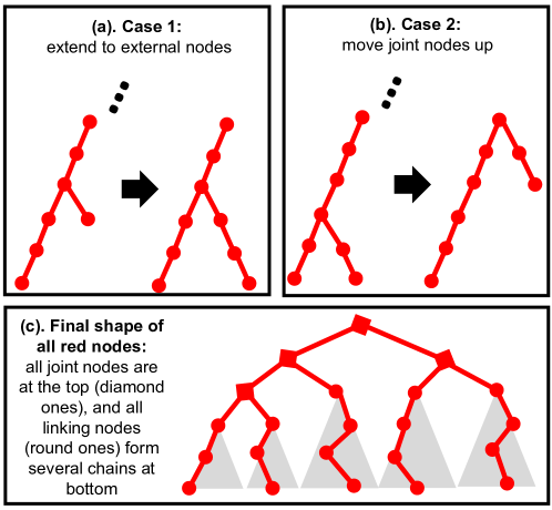
Figure 8: An illustration about adjusting red nodes in Proof B.1. (a) Extend all inner joint nodes to some external node. (b) Move all joint nodes to upper levels as far as possible. (c) The final shape after adjusting the red nodes. All joint nodes are at the top, and all linking nodes form chains at bottom.

Proof.

First of all, we find all the searching paths to all the $m$ elements, and mark all related nodes on the path as red. All the red nodes form a tree structure, which is a connected component of $T$. We then adjust the red nodes, such that the number of red nodes does not decrease. We define a red node with two red children as a joint node, and a red node with one red child as a linking node.

1. First, as shown in Figure 8 (a), any of the red nodes are internal nodes in $T$, we arbitrarily extend it to some external node in the tree.

2. Second, as shown in Figure 8 (b), if there is any linking node $v$ with some joint nodes as its descendent, then we move the first joint node of its descendants up to replace the non-red child of $v$.

We repeat the two steps until there is no such situations. These adjustments only make the total number of red nodes larger. Finally we will have all joint nodes on the top levels of the tree, forming a connected component. All the linking nodes form several (at most $m$) chains at the bottom levels. The total number of joint nodes is $O(m)$ because the number of chains is at most $m$. For all the linking nodes, they form several chains. These chains starts from a linking node $u_{i}$ whose parent is a joint node $p(u_{i})$. All such $p(u_{i})$ nodes have disjoint subtrees. We assume the size of $p(u_{i})$ is $n_{i}$, then we have $\sum_{i=1}^{m}n_{i}\leq n$. The total length of all chains is:

$$\sum_{i=1}^{m}\log(n_{i}+1)\leq m\log\mathopen{}\mathclose{{}\left(\frac{\sum_{i=1}^{m}n_{i}+1}{m}}\right)\leq m\log\mathopen{}\mathclose{{}\left(\frac{n}{m}+1}\right)$$

The above inequality can be shown by the Jensen’s inequality. ∎

Lemma B.2.

Let $\sum_{i=1}^{k}m_{i}=m$, $\sum_{i=1}^{k}n_{i}=n$ and $\forall i,m_{i},n_{i}\in\mathbb{Z^{+}},m_{i}<\sqrt{n_{i}+m_{i}}$, then we have $\sum_{i=1}^{k}m_{i}\log n_{i}\in O\mathopen{}\mathclose{{}\left(m\log\mathopen{}\mathclose{{}\left(\frac{n}{m}+1}\right)}\right)$.

Proof of Lemma B.2.

We will show that given the conditions above, the maximum value of $\sum_{i=1}^{k}m_{i}\log n_{i}$ is no more than $cm\log\mathopen{}\mathclose{{}\left(\frac{n}{m}+1}\right)$ for some constant $c$. This follows the observation that $m_{i}\log n_{i}+m_{j}\log n_{j}$ gets the maximum value when $\frac{n_{i}}{n_{j}}=\frac{m_{i}}{m_{j}}$, given $n_{i}+n_{j}$ is fixed. Then for any two terms $n_{i}$ and $n_{j}$ on the left-hand side of the equation, if $n_{i}$ and $n_{j}$ are not distributed as the ratio of $m_{i}/m_{j}$, we re-distribute them as so, and the objective will never decrease. Thus the maximum value of the objective is when $n_{i}=\frac{m_{i}}{m}n$. This might invalidate the condition that $m_{i}<\sqrt{n_{i}+m_{i}}$, but will only make the bound looser. In this case, $m_{i}<\sqrt{n_{i}+m_{i}}<\sqrt{2n_{i}}=\sqrt{\frac{2m_{i}}{m}n}$, leading to $m_{i}<{2n\over m}$. Then we have:

$$\sum_{i=1}^{k}m_{i}\log n_{i} \leq\sum_{i=1}^{k}m_{i}\log\frac{m_{i}}{m}n$$

$$=\sum_{i=1}^{k}m_{i}\log\frac{n}{m}+\sum_{i=1}^{k}m_{i}\log{m_{i}}$$

$$<m\log\frac{n}{m}+\sum_{i=1}^{k}m_{i}\log{\frac{2n}{m}}$$

$$\in O\mathopen{}\mathclose{{}\left(m\log\mathopen{}\mathclose{{}\left(\frac{n}{m}+1}\right)}\right)$$

∎

Lemma B.3.

For a binary tree $T$, if its left and right subtrees are both valid WBB[$\alpha$] trees, and their weights differ by no more than $2/\alpha$, then we can rebalance $T$ as a WBB[$\alpha$] tree by a constant number of rotations, given $0<\alpha\leq 1-1/\sqrt{2}$.

Lemma B.3 is a special case of Lemma 3 in [21] and can be proved in a similar way as shown in [21].

B.2 The Proof for Theorem 5.1

We now prove the cost bound of Algorithm 3. Although Algorithm 3 is not very complicated, the analysis is reasonably involved, especially when we need to analyze all three different ordered set operations. We first analyze the span in Lemma B.6, and the work bounds for the sketch step (Algorithm 4) in Lemma B.8, and the rebalance step (Algorithm 5) in Lemma B.9. Combining these three lemmas proves the theorem.

Recall in the divide-and-conquer algorithm, we use pivots (or splitters) to split the input trees to subproblems, and connect them back regardless of balance. We do so until reaching the base cases. As a result, all pivots in the algorithm form the upper levels of the sketch $T^{\prime}$. We refer to these upper levels containing all the pivots throughout the algorithm as the skeleton of $T^{\prime}$. The skeleton consists of a connected collection of full binary trees of different sizes. We first show two useful lemmas, revealing some useful information about the sketch tree $T^{\prime}$. We first bound the size of the skeleton of $T^{\prime}$.

Lemma B.4.

For two input trees of sizes $m$ and $n\geq m$, there are in total $O(m)$ pivots in Algorithm 4.

Proof.

We look at the tree skeleton consisting of all pivots in the algorithm. We will show that there at most $O(m)$ leaves in this skeleton. Each leaf corresponds to a function call of the base case. For any two sibling leafs, at least one of the elements in $T_{S}$ must fall into one of the two base cases, otherwise the algorithm should come to the base case on the upper level. This means that there can be at most $2m$ base cases. ∎

Intuitively, this is because when there are more than $m$ pivots, some of them must have an empty $T_{2}$ as input, which goes to the base case (Line 4 in Algorithm 4) immediately.

We then bound the height of all subtrees in the sketch tree $T^{\prime}$.

Lemma B.5.

(Subtree height in sketch tree $T^{\prime}$) For any subtree in $T^{\prime}$ obtained by the sketching step in Algorithm 3, the height is no more than $O(\log n^{\prime})$ for a subtree of size $n^{\prime}$.

Proof.

For any subtree $T_{x}\in T^{\prime}$, there are two parts. The first several upper levels are in the skeleton, and the bottom several levels are those obtained by base cases. For the base case subtrees, they are balanced, and thus the height is at most $O(\log n^{\prime})$. For the skeleton, it consists of several full binary trees of size $d$, for different $d$ values of recursion calls. Assume on the topmost (complete) level it is $d_{0}$-way dividing, so the first several levels should be a full binary tree of height $O(\log_{2}d_{0})$. Then for the next levels, it is at most $\sqrt{d_{0}}$-way, so the height is at most $\log_{2}\sqrt{d_{0}}$. So on so forth. There also can be an incomplete full binary tree above $d_{0}$, and the height can be at most $\log_{2}d_{0}$. Therefore the height of the skeleton is at most $2\log_{2}d_{0}+\log_{2}\sqrt{d_{0}}+\dots=O(\log d_{0})=O(\log n)$. ∎

This is guaranteed by the base case algorithms and the connecting substep of the Sketching step.

We now prove the span of the algorithm. Intuitively, the sketching step is a $\sqrt{n+m}$-way recursion, and thus requires logarithmic span. For the rebalancing step, either reconstruction or rebalance by rotations costs a constant amortized time per level. We formally show the following lemma.

Lemma B.6.

Algorithm 3 has span $O(\log n)$ in the binary-forking model.

Proof.

We first look at the Sketching step working on two trees of size $n^{\prime}$ (from the original large tree) and $m^{\prime}$ (from the original small tree). The span for finding $d-1$ pivots, checking tombs, splitting, and the connecting functions are all $O(\log(n^{\prime}+m^{\prime}))$. For the next level of recursive call, the size of the problem shrink to $\sqrt{m^{\prime}+n^{\prime}}$. The span of a base case is also $O(\log(m^{\prime}+n^{\prime}))$. The recursion is therefore:

$$T(m+n)=c_{1}\log(m+n)+T(\sqrt{m+n})$$

The solution is $T(m+n)\in O(\log(m+n))$.

For the Rebalancing step. We show this by induction that the span to rebalance a tree $T$ obtained by the sketching step is $O(\log|T|)$. The base case is straightforward. Other than the base case, there are two cases.

If a subtree has its left and right children unbalanced, we need to reconstruct the tree structure. This requires to flatten all elements in an array and then build a complete binary tree on top of the array. The span of this step is no more than the height of the tree, which, according to Lemma B.5, is $O(\log|T|)$.

Otherwise, each of the left and right subtrees has no more than $c|T|$ elements for some constant $c<1$. Rebalancing each of them, according to the inductive hypothesis, only need span $O(\log c|T|)$. There is an extra cost in rebalancing at the root of $T$ by rotation, which is constant time.

For both cases, settling the subtree $T$ cost span $O(\log|T|)$. For our algorithm, it is $O(\log(m+n))=O(\log n)$. ∎

Next we prove the work of the algorithm, we start with showing that the total work of all bases cases is $O\mathopen{}\mathclose{{}\left(m\log\mathopen{}\mathclose{{}\left(\frac{n}{m}+1}\right)}\right)$.

Lemma B.7.

For two input trees of sizes $m$ and $n\geq m$, all base cases in Algorithm 3 require $O\mathopen{}\mathclose{{}\left(m\log\mathopen{}\mathclose{{}\left(\frac{n}{m}+1}\right)}\right)$ work.

Outline.

All the non-trivial base cases are when $m^{\prime}<\sqrt{n^{\prime}}$ in the recursive calls, which will directly invoke the base case algorithms shown in Section A. All such base case algorithms have $O(m^{\prime}\log n^{\prime})$ work. Suppose there are $k$ such base case calls, each with input size $m_{i}$ and $n_{i}$ for $1\leq i\leq k$, where $\sum n_{i}=n,\sum m_{i}=m$ and $m_{i}<\sqrt{n_{i}+m_{i}}$. Then the total work is asymptotically $\sum_{i=1}^{k}m_{i}\log n_{i}$, which is $O(O\mathopen{}\mathclose{{}\left(m\log\mathopen{}\mathclose{{}\left(\frac{n}{m}+1}\right)}\right))$ based on Lemma B.2. ∎

Next, we prove that the sketching step (Algorithm 4) uses work $O\mathopen{}\mathclose{{}\left(m\log\mathopen{}\mathclose{{}\left(\frac{n}{m}+1}\right)}\right)$. This process is a leaf-dominated recursion and thus the total work is bounded by all bases cases.

Lemma B.8.

The sketching step (Algorithm 4) has $O\mathopen{}\mathclose{{}\left(m\log\mathopen{}\mathclose{{}\left(\frac{n}{m}+1}\right)}\right)$ work.

Proof.

First of all, for all base cases, the total cost is $O\mathopen{}\mathclose{{}\left(m\log\mathopen{}\mathclose{{}\left(\frac{n}{m}+1}\right)}\right)$ based on Lemma B.7.

Excluding the base cases, we now look at the work caused by the sketching step on two trees of size $n^{\prime}$ (from the original large tree) and $m^{\prime}$ (from the original small tree).

In the parallel-for loops, the main work are for 1) finding the splitters, 2) splitting each tree into $d$ pieces and checking if each splitter is a tomb. All these cost work $O(\sqrt{n^{\prime}+m^{\prime}}\log(n^{\prime}+m^{\prime}))$. Then there will be $d\approx\sqrt{n^{\prime}+m^{\prime}}$ recursive calls, each with size about $\sqrt{n^{\prime}+m^{\prime}}$.

For all connecting steps, since there are at most $O(m)$ base cases, there are at most $O(m)$ connecting pivots. Each connection costs a constant time, which means that this part only costs work $O(m)$.

We then prove that the total work in parallel for loops is also $O\mathopen{}\mathclose{{}\left(m^{\prime}\log\frac{n^{\prime}}{m^{\prime}}}\right)$. Consider the recurrence tree of this algorithm, which has $\sqrt{m^{\prime}+n^{\prime}}$-way fan-out for a recursion with sizes $n^{\prime}$ and $m^{\prime}$, and the cost of the current node is $\sqrt{n^{\prime}+m^{\prime}}\log(n^{\prime}+m^{\prime})$. In our algorithm, we stop recursing when $m^{\prime}\geq\sqrt{m^{\prime}+n^{\prime}}$ and call the base case algorithm instead of waiting until $m^{\prime}$ or $n^{\prime}$ reaches zero. As a result, the tree is not perfectly balanced. Some branches can be shallow (reaching base cases earlier) and some can be deep (reaching base cases later). The cost at each node, however, is exactly the same in the same level, but decreases as the tree goes deeper. Therefore, given the number of leaves fixed, the worst case occurs when all nodes are at the topmost several levels. Let $t=m^{\prime}+n^{\prime}$, the total work for these operations is:

$$t^{1/2}\log t+t^{1/2}\cdot t^{1/4}\log t^{1/2}+t^{1/2}\cdot t^{1/4}\cdot t^{1/8}\log t^{1/4}+\dots$$

$$= \sum\frac{\log t}{2^{i}}t^{1-1/2^{i+1}}$$

This recurrence is leaf-dominated. The recurrence suggested that in the $i$-th term, there are $t^{1-1/2^{i+1}}$ subtasks each costing $\frac{\log t}{2^{i}}$ work. We then want to know, when the recurrence stops, how much work we pay. From Lemma B.4, we know the total number of pivots is no more than $m^{\prime}$, and thus $t^{1-1/2^{i+1}}\leq m^{\prime}$. Let $x=t^{1/2^{i+1}}$, the total leaf cost is asymptotically

$$t^{1-1/2^{i+1}}\log t^{1/2^{i+1}}=\frac{t}{x}\log x$$

Given $t$ fixed, this function is decreasing when $x\rightarrow+\infty$. Considering $t^{1-1/2^{i+1}}\leq m^{\prime}$, we know that $x\geq t/m^{\prime}$. Plug in $x=t/m^{\prime}$ we know that the total work is at most

$$O\mathopen{}\mathclose{{}\left(\frac{t}{x}\log x}\right)=O\mathopen{}\mathclose{{}\left(m^{\prime}\log\frac{t}{m^{\prime}}}\right)=O\mathopen{}\mathclose{{}\left(m^{\prime}\log\frac{n^{\prime}+m^{\prime}}{m^{\prime}}}\right)=O\mathopen{}\mathclose{{}\left(m^{\prime}\log\frac{n^{\prime}}{m^{\prime}}}\right)$$

Therefore, the work of the sketching step is $O\mathopen{}\mathclose{{}\left(m\log\mathopen{}\mathclose{{}\left(\frac{n}{m}+1}\right)}\right)$. ∎

Finally, we show the total work of rebalancing is $O\mathopen{}\mathclose{{}\left(m\log\mathopen{}\mathclose{{}\left(\frac{n}{m}+1}\right)}\right)$. Intuitively, this is because the amortized time to settle a tree node is a constant for either rotation or rebalancing. In addition, for filling in all tombs, the total work is $O\mathopen{}\mathclose{{}\left(m\log\mathopen{}\mathclose{{}\left(\frac{n}{m}+1}\right)}\right)$. We formally prove it as follows.

Lemma B.9.

The rebalancing step (Algorithm 5) has $O\mathopen{}\mathclose{{}\left(m\log\mathopen{}\mathclose{{}\left(\frac{n}{m}+1}\right)}\right)$ work.

Proof.

We first show that for Union we do not need to rebalance. If there are no duplicates in the two input sets, all the chunks are of the same size. Considering the duplicates, the size of each chunk can shrink by at most a half. In this case, and since the pivots perfectly balance not considering duplicates, the tree is still balanced under the weight-balanced invariant.

We then consider Intersection and Difference. In Algorithm 5, the total work consists of three parts: filling up the tombs (Line 5 and 5), reconstruction (Line 5), and rotation (Line 5). We note them as $W_{1}$, $W_{2}$ and $W_{3}$, respectively.

We first prove that $W_{2}+W_{3}$ is $O\mathopen{}\mathclose{{}\left(m\log\mathopen{}\mathclose{{}\left(\frac{n}{m}+1}\right)}\right)$. We ignore the cost of RemoveLast for now. Note that all subtrees obtained by base cases are balanced, so the rebalancing process will not touch those parts in $T^{\prime}$ (Line 5 in Algorithm 5), and will only visit the pivots in the skeleton.

For all elements $k\in T_{S}$, we mark all their upper nodes in $T^{\prime}$ as red. If there is no element $k\in T_{S}$ falling into a subtree in $T^{\prime}$, this subtree will be skipped over directly (Line 5). Therefore the red nodes are the only nodes visited by the algorithm for reconstruction and rotation.

Based on Lemma B.1 and Lemma B.5, there are at most $O\mathopen{}\mathclose{{}\left(m\log\mathopen{}\mathclose{{}\left(\frac{n}{m}+1}\right)}\right)$ such red nodes in the skeleton. We denote the number of red nodes in a subtree $T$ (or a subtree rooted at $v$) as $R(T)$ (or $R(v)$). We first show that if we do not consider the cost of filling the tombs, the rebalancing cost for any subtree $T_{x}\in T^{\prime}$ is asymptotically no more than $R(T_{x})$. We show this by induction.

First, only those red nodes will be reached in the rebalancing step. Therefore the base case holds (e.g., when the tree is just one red node). For each red node $v$ in $T^{\prime}$, there are two cases.

1. $v$’s left and right subtrees are almost balanced. In this case $v$ will be settled by a constant number of rotations. Considering the inductive hypothesis, the total work is asymptotically no more than the number of red nodes in the whole subtree.

2. The sizes of $v$’s left and right subtrees differ by more than a constant factor $c$. Then we need to reconstruct the subtree, and the work is linear to the size of $v$’s subtree. We use $M$ to represent the number of elements in $T_{S}$ that fall into $v$’s subtree.

   We first show $M\leq R(v)$. This is because the red nodes are always ancestors (inclusive) of those tree nodes from $T_{S}$. Therefore, $M\leq R(v)$ holds for all tree nodes $v$.

   Recall that all the chunks are designed to be of the same size. For Union (i.e., no tombs in the tree), the size of two chunks can differ by at most a factor of two (due to duplicates), which will not cause imbalance. For Difference and Intersection, the only reason for the imbalance is that there are tombs being removed. There are two cases. We next show that in either case, the difference between the left subtree and right subtree of $v$ is no more than $M$.

   1. In Difference ($T_{L}-T_{S}$). All tombs are elements in $T_{S}$. In these case, the difference of the left subtree and right subtree of $v$ is no more than $M$.

   2. In Difference ($T_{S}-T_{L}$) and Intersection. In these two cases all elements in $v$’s subtree must appear in $T_{S}$. Thus the size of the whole subtree (excluding tombs) rooted at $v$ is no more than $M$, and therefore the difference of the left subtree and right subtree of $v$ is no more than $M$.

   Recall that we use $l(v)$ and $r(v)$ to denote the left and right subtrees of a node $v$, respectively. Therefore the above statements proves that $c\cdot\text{size}(v)\leq|\text{size}(r(v))-\text{size}(l(v))|\leq M\leq R(v)$, for some constant $c$. Therefore, the total work $O(\text{size}(v))$ is also $O(R(v))$.

Therefore we proved that in any of the subtree $T_{x}\in T^{\prime}$ the work is asymptotically no more than $R(T_{x})$. This will also be true for $T^{\prime}$ itself, and $W_{2}+W_{3}$ for whole $T^{\prime}$ is $O\mathopen{}\mathclose{{}\left(m\log\mathopen{}\mathclose{{}\left(\frac{n}{m}+1}\right)}\right)$.

Next we show that $W_{1}$ is $O\mathopen{}\mathclose{{}\left(m\log\mathopen{}\mathclose{{}\left(\frac{n}{m}+1}\right)}\right)$. For $W_{3}$, the algorithm will pop up at most $m$ elements to fill in the tombs. Each such operation follows the right spine in the corresponding subtree of size $n^{\prime}$ in $O(\log n^{\prime})$ time. All such subtrees are disjoint. Therefore, based on Lemma B.2, the total cost is $O\mathopen{}\mathclose{{}\left(m\log\mathopen{}\mathclose{{}\left(\frac{n}{m}+1}\right)}\right)$. ∎

Combining Lemmas B.7, B.8 and B.9 gives the following Lemma about the work of Algorithm 3.

Lemma B.10.

The total work of Algorithm 3 is $O\mathopen{}\mathclose{{}\left(m\log\mathopen{}\mathclose{{}\left(\frac{n}{m}+1}\right)}\right)$.

Lemma B.9 also indicates the following corollary:

Corollary B.11.

Rebalance$(T,\texttt{false})$ as shown in Algorithm 5 on a weight-balanced tree $T$ of size $n$ with $m$ tombs in it cost work $O\mathopen{}\mathclose{{}\left(m\log\mathopen{}\mathclose{{}\left(\frac{n}{m}+1}\right)}\right)$. For this case we ignore the part of if-condition about base case at line 5.

This corollary is weaker than the condition considered in Lemma B.9, and thus can be shown using a similar proof. This corollary can be used to bound the work of the base case and the work for Union and Difference (see Section A). Combining Lemmas B.6–B.9 gives Theorem 5.1.

Appendix C Proof of Theorem 2.2

Proof.

(Outline). The first inclusion is well known [35]. To simulate $L$ in $\mathcal{BF}^{1}$ we can construct a graph representing the state transition diagram of the logspace computation. Each state looks at one bit of the input tape and has two edges out, one for 0 and one for 1. The construction is logspace uniform. For a particular input of length $n$ we select the appropriate edges, which forms a forest with the accept states appearing as some of the roots. An Euler Tour can be built on the trees in the forest—not hard to do in logarithmic span. Using deterministic list-contraction, as described at the end of the next section, the simulation can identify if the start state has an accept state as its root. The full computation has $O(\log n)$ span and does polynomial work (there are polynomially many states).

To simulate $\mathcal{BF}^{1}$ in $\mathcal{AC}^{1}$ we could use know results for simulating the CRCW PRAM in circuit depth proportional to time [39], but this would require randomization since our simulation of the binary-forking model on the PRAM uses randomization. However, it is not difficult to extend the ideas for a deterministic simulation. The idea is that the shared memory can be simulated in constant depth per step [75], as can the processor. The processor simulation can take advantage of the fact that our registers only have $O(\log n)$ bits and instructions only take a constant number of registers. This allows instructions to be simulated in constant depth and polynomial size, effectively by table lookup (just index the correct solution based on the $O(\log n)$ input bits). The forking can be simulated by assuming that every instruction might be a fork, so create circuits for two copies of the processor as the children of each instruction. Since the computation has $O(\log n)$ span, at most a polynomial number of processors simulators are required in the circuit.

∎

References

- [1] Umut A. Acar, Guy E. Blelloch, and Robert D. Blumofe. The data locality of work stealing. Theoretical Computer Science (TCS), 35(3), 2002.
- [2] Umut A. Acar, Arthur Charguéraud, Adrien Guatto, Mike Rainey, and Filip Sieczkowski. Heartbeat scheduling: Provable efficiency for nested parallelism. In ACM Conference on Programming Language Design and Implementation (PLDI), pages 769–782, 2018.
- [3] Kunal Agrawal, Jeremy T. Fineman, Kefu Lu, Brendan Sheridan, Jim Sukha, and Robert Utterback. Provably good scheduling for parallel programs that use data structures through implicit batching. In ACM Symposium on Parallelism in Algorithms and Architectures (SPAA), 2014.
- [4] Kunal Agrawal, Seth Gilbert, and Wei Quan Lim. Parallel working-set search structures. In ACM Symposium on Parallelism in Algorithms and Architectures (SPAA), 2018.
- [5] Yaroslav Akhremtsev and Peter Sanders. Fast parallel operations on search trees. In IEEE International Conference on High Performance Computing (HiPC), 2016.
- [6] Laurent Alonso and Ren Schott. A parallel algorithm for the generation of a permutation and applications. Theoretical Computer Science (TCS), 159(1), 1996.
- [7] Stephen Alstrup, Cyril Gavoille, Haim Kaplan, and Theis Rauhe. Nearest common ancestors: A survey and a new algorithm for a distributed environment. Theory of Computing Systems (TOCS), 37(3):441–456, 2004.
- [8] Richard J. Anderson. Parallel algorithms for generating random permutations on a shared memory machine. In ACM Symposium on Parallelism in Algorithms and Architectures (SPAA), 1990.
- [9] Richard J Anderson and Gary L Miller. A simple randomized parallel algorithm for list-ranking. Information Processing Letters, 33(5):269–273, 1990.
- [10] Lars Arge, Johannes Fischer, Peter Sanders, and Nodari Sitchinava. On (dynamic) range minimum queries in external memory. In Workshop on Algorithms and Data Structures, pages 37–48. Springer, 2013.
- [11] N. S. Arora, R. D. Blumofe, and C. G. Plaxton. Thread scheduling for multiprogrammed multiprocessors. Theory of Computing Systems (TOCS), 34(2), Apr 2001.
- [12] Sara Baase. Introduction to parallel connectivity, list ranking, and Euler tour techniques. In John Reif, editor, Synthesis of Parallel Algorithms, pages 61–114. Morgan Kaufmann, 1993.
- [13] Naama Ben-David, Guy E. Blelloch, Jeremy T. Fineman, Phillip B. Gibbons, Yan Gu, Charles McGuffey, and Julian Shun. Parallel algorithms for asymmetric read-write costs. In ACM Symposium on Parallelism in Algorithms and Architectures (SPAA), 2016.
- [14] Naama Ben-David, Guy E. Blelloch, Jeremy T Fineman, Phillip B Gibbons, Yan Gu, Charles McGuffey, and Julian Shun. Implicit decomposition for write-efficient connectivity algorithms. In IEEE International Parallel and Distributed Processing Symposium (IPDPS), 2018.
- [15] Michael A. Bender, Alex Conway, Martín Farach-Colton, William Jannen, Yizheng Jiao, Rob Johnson, Eric Knorr, Sara McAllister, Nirjhar Mukherjee, Prashant Pandey, et al. Small refinements to the DAM can have big consequences for data-structure design. In ACM Symposium on Parallelism in Algorithms and Architectures (SPAA), pages 265–274, 2019.
- [16] Michael A. Bender and Martin Farach-Colton. The lca problem revisited. In Latin American Symposium on Theoretical Informatics (LATIN), pages 88–94. Springer, 2000.
- [17] Omer Berkman and Uzi Vishkin. Recursive star-tree parallel data structure. SIAM J. Scientific Computing, 22(2):221–242, 1993.
- [18] Guy E. Blelloch. Prefix sums and their applications. In John Reif, editor, Synthesis of Parallel Algorithms. Morgan Kaufmann, 1993.
- [19] Guy E. Blelloch. Programming parallel algorithms. Commun. ACM, 39(3), March 1996.
- [20] Guy E. Blelloch, Rezaul Alam Chowdhury, Phillip B. Gibbons, Vijaya Ramachandran, Shimin Chen, and Michael Kozuch. Provably good multicore cache performance for divide-and-conquer algorithms. In ACM-SIAM Symposium on Discrete Algorithms (SODA), 2008.
- [21] Guy E. Blelloch, Daniel Ferizovic, and Yihan Sun. Just join for parallel ordered sets. In ACM Symposium on Parallelism in Algorithms and Architectures (SPAA), 2016.
- [22] Guy E. Blelloch, Jeremy T. Fineman, Phillip B. Gibbons, and Julian Shun. Internally deterministic parallel algorithms can be fast. In ACM Symposium on Principles and Practice of Parallel Programming (PPOPP), 2012.
- [23] Guy E. Blelloch, Jeremy T. Fineman, Phillip B. Gibbons, and Harsha Vardhan Simhadri. Scheduling irregular parallel computations on hierarchical caches. In ACM Symposium on Parallelism in Algorithms and Architectures (SPAA), 2011.
- [24] Guy E. Blelloch and Phillip B. Gibbons. Effectively sharing a cache among threads. In ACM Symposium on Parallelism in Algorithms and Architectures (SPAA), 2004.
- [25] Guy E. Blelloch, Phillip B. Gibbons, and Yossi Matias. Provably efficient scheduling for languages with fine-grained parallelism. J. ACM, 46(2), March 1999.
- [26] Guy E. Blelloch, Phillip B. Gibbons, and Harsha Vardhan Simhadri. Low depth cache-oblivious algorithms. In ACM Symposium on Parallelism in Algorithms and Architectures (SPAA), 2010.
- [27] Guy E. Blelloch, Yan Gu, Julian Shun, and Yihan Sun. Parallelism in randomized incremental algorithms. In ACM Symposium on Parallelism in Algorithms and Architectures (SPAA), 2016.
- [28] Guy E. Blelloch, Yan Gu, Julian Shun, and Yihan Sun. Parallel write-efficient algorithms and data structures for computational geometry. In ACM Symposium on Parallelism in Algorithms and Architectures (SPAA), 2018.
- [29] Guy E. Blelloch, Yan Gu, Julian Shun, and Yihan Sun. Randomized incremental convex hull is highly parallel. In ACM Symposium on Parallelism in Algorithms and Architectures (SPAA), 2020.
- [30] Guy E. Blelloch and Margaret Reid-Miller. Fast set operations using treaps. In ACM Symposium on Parallelism in Algorithms and Architectures (SPAA), 1998.
- [31] Guy E. Blelloch and Margaret Reid-Miller. Pipelining with futures. Theory of Computing Systems (TOCS), 32(3), 1999.
- [32] Guy E. Blelloch, Harsha Vardhan Simhadri, and Kanat Tangwongsan. Parallel and I/O efficient set covering algorithms. In ACM Symposium on Parallelism in Algorithms and Architectures (SPAA), 2012.
- [33] Robert D. Blumofe and Charles E. Leiserson. Space-efficient scheduling of multithreaded computations. SIAM J. Scientific Computing, 27(1), 1998.
- [34] Robert D. Blumofe and Charles E. Leiserson. Scheduling multithreaded computations by work stealing. J. ACM, 46(5):720–748, 1999.
- [35] Allan Borodin. On relating time and space to size and depth. SIAM J. Scientific Computing, 6(4):733–744, 1977.
- [36] Anastasia Braginsky and Erez Petrank. A lock-free b+ tree. In ACM Symposium on Parallelism in Algorithms and Architectures (SPAA), pages 58–67, 2012.
- [37] Mark R. Brown and Robert Endre Tarjan. Design and analysis of a data structure for representing sorted lists. SIAM J. Scientific Computing, 9(3):594–614, 1980.
- [38] Zoran Budimlić, Vincent Cavé, Raghavan Raman, Jun Shirako, Sağnak Taşırlar, Jisheng Zhao, and Vivek Sarkar. The design and implementation of the habanero-java parallel programming language. In Symposium on Object-oriented Programming, Systems, Languages and Applications (OOPSLA), pages 185–186, 2011.
- [39] Ashok K. Chandra, Larry J. Stockmeyer, and Uzi Vishkin. Constant depth reducibility. SIAM J. Comput., 13(2):423–439, 1984.
- [40] Philippe Charles, Christian Grothoff, Vijay Saraswat, Christopher Donawa, Allan Kielstra, Kemal Ebcioglu, Christoph Von Praun, and Vivek Sarkar. X10: an object-oriented approach to non-uniform cluster computing. In ACM SIGPLAN Conference on Object-oriented Programming, Systems, Languages, and Applications (OOPSLA), pages 519–538, 2005.
- [41] Rezaul Chowdhury, Pramod Ganapathi, Yuan Tang, and Jesmin Jahan Tithi. Provably efficient scheduling of cache-oblivious wavefront algorithms. In ACM Symposium on Parallelism in Algorithms and Architectures (SPAA), pages 339–350, 2017.
- [42] Rezaul A. Chowdhury, Vijaya Ramachandran, Francesco Silvestri, and Brandon Blakeley. Oblivious algorithms for multicores and networks of processors. Journal of Parallel and Distributed Computing, 73(7):911–925, 2013.
- [43] Richard Cole. Parallel merge sort. SIAM J. Scientific Computing, 17(4), 1988.
- [44] Richard Cole and Vijaya Ramachandran. Bounding cache miss costs of multithreaded computations under general schedulers: Extended abstract. In ACM Symposium on Parallelism in Algorithms and Architectures (SPAA), 2017.
- [45] Richard Cole and Vijaya Ramachandran. Resource oblivious sorting on multicores. ACM Transactions on Parallel Computing (TOPC), 3(4), 2017.
- [46] Richard Cole and Uzi Vishkin. Deterministic coin tossing and accelerating cascades: Micro and macro techniques for designing parallel algorithms. In ACM Symposium on Theory of Computing (STOC), pages 206–219, 1986.
- [47] Richard Cole and Uzi Vishkin. Approximate parallel scheduling. part i: The basic technique with applications to optimal parallel list ranking in logarithmic time. SIAM J. Scientific Computing, 17:128–142, 1988.
- [48] Richard Cole and Uzi Vishkin. Faster optimal parallel prefix sums and list ranking. Information and computation, 81(3):334–352, 1989.
- [49] Guojing Cong and David A. Bader. An empirical analysis of parallel random permutation algorithms on SMPs. In Parallel and Distributed Computing and Systems (PDCS), 2005.
- [50] Thomas H. Cormen, Charles E. Leiserson, Ronald L. Rivest, and Clifford Stein. Introduction to Algorithms (3rd edition). MIT Press, 2009.
- [51] Artur Czumaj, Przemyslawa Kanarek, Miroslaw Kutylowski, and Krzysztof Lorys. Fast generation of random permutations via networks simulation. Algorithmica, 1998.
- [52] Laxman Dhulipala, Guy E. Blelloch, and Julian Shun. Theoretically efficient parallel graph algorithms can be fast and scalable. In ACM Symposium on Parallelism in Algorithms and Architectures (SPAA), 2018.
- [53] Laxman Dhulipala, Charlie McGuffey, Hongbo Kang, Yan Gu, Guy E Blelloch, Phillip B Gibbons, and Julian Shun. Semi-asymmetric parallel graph algorithms for nvrams. Proceedings of the VLDB Endowment (PVLDB), 13(9), 2020.
- [54] David Dinh, Harsha Vardhan Simhadri, and Yuan Tang. Extending the nested parallel model to the nested dataflow model with provably efficient schedulers. In ACM Symposium on Parallelism in Algorithms and Architectures (SPAA), 2016.
- [55] James R. Driscoll, Neil Sarnak, Daniel D. Sleator, and Robert E. Tarjan. Making data structures persistent. J. Computer and System Sciences, 38(1):86–124, 1989.
- [56] Richard Durstenfeld. Algorithm 235: Random permutation. Commun. ACM, 7(7):420, 1964.
- [57] Panagiota Fatourou, Elias Papavasileiou, and Eric Ruppert. Persistent non-blocking binary search trees supporting wait-free range queries. In ACM Symposium on Parallelism in Algorithms and Architectures (SPAA), pages 275–286, 2019.
- [58] Johannes Fischer and Volker Heun. Theoretical and practical improvements on the RMQ-problem, with applications to LCA and LCE. In Symposium on Combinatorial Pattern Matching (CPM), pages 36–48. Springer, 2006.
- [59] W Donald Frazer and Archie C McKellar. Samplesort: A sampling approach to minimal storage tree sorting. J. ACM, 17(3):496–507, 1970.
- [60] Matteo Frigo, Charles E. Leiserson, and Keith H. Randall. The implementation of the cilk-5 multithreaded language. ACM SIGPLAN Conference on Programming Language Design and Implementation (PLDI), 33(5):212–223, 1998.
- [61] Phillip B. Gibbons, Yossi Matias, and Vijaya Ramachandran. Efficient low-contention parallel algorithms. J. Computer and System Sciences, 53(3), 1996.
- [62] Joseph Gil. Fast load balancing on a PRAM. In IEEE International Parallel and Distributed Processing Symposium (IPDPS), 1991.
- [63] Joseph Gil, Yossi Matias, and Uzi Vishkin. Towards a theory of nearly constant time parallel algorithms. In IEEE Symposium on Foundations of Computer Science (FOCS), 1991.
- [64] Seth Gilbert and Wei Quan Lim. Parallel finger search structures. arXiv preprint arXiv:1908.02741, 2019.
- [65] Yan Gu, Julian Shun, Yihan Sun, and Guy E Blelloch. A top-down parallel semisort. In ACM Symposium on Parallelism in Algorithms and Architectures (SPAA), 2015.
- [66] Jens Gustedt. Randomized permutations in a coarse grained parallel environment. In ACM Symposium on Parallelism in Algorithms and Architectures (SPAA), 2003.
- [67] Jens Gustedt. Engineering parallel in-place random generation of integer permutations. In Workshop on Experimental Algorithmics, 2008.
- [68] Torben Hagerup. Fast parallel generation of random permutations. In Intl. Colloq. on Automata, Languages and Programming (ICALP). Springer, 1991.
- [69] Maurice Herlihy. Wait-free synchronization. ACM Transactions on Programming Languages and Systems (TOPLAS), 13(1):124–149, 1991.
- [70] Frank K. Hwang and Shen Lin. A simple algorithm for merging two disjoint linearly ordered sets. SIAM J. Scientific Computing, 1(1):31–39, 1972.
- [71] https://www.threadingbuildingblocks.org.
- [72] Riko Jacob, Tobias Lieber, and Nodari Sitchinava. On the complexity of list ranking in the parallel external memory model. In International Symposium on Mathematical Foundations of Computer Science, pages 384–395. Springer, 2014.
- [73] J. JaJa. Introduction to Parallel Algorithms. Addison-Wesley Professional, 1992.
- [74] http://docs.oracle.com/javase/tutorial/essential/concurrency/forkjoin.html.
- [75] Richard M. Karp and Vijaya Ramachandran. Parallel algorithms for shared-memory machines. In Handbook of Theoretical Computer Science, Volume A: Algorithms and Complexity (A). MIT Press, 1990.
- [76] Donald E. Knuth. The Art of Computer Programming, Volume II: Seminumerical Algorithms. Addison-Wesley, 1969.
- [77] Gary L. Miller and John H. Reif. Parallel tree contraction and its application. In IEEE Symposium on Foundations of Computer Science (FOCS), pages 478–489, 1985.
- [78] Gal Milman, Alex Kogan, Yossi Lev, Victor Luchangco, and Erez Petrank. Bq: A lock-free queue with batching. In ACM Symposium on Parallelism in Algorithms and Architectures (SPAA), pages 99–109, 2018.
- [79] Jürg Nievergelt and Edward M Reingold. Binary search trees of bounded balance. SIAM J. Scientific Computing, 2(1), 1973.
- [80] Heejin Park and Kunsoo Park. Parallel algorithms for red-black trees. Theoretical Computer Science (TCS), 262(1–2):415–435, 2001.
- [81] Wolfgang J. Paul, Uzi Vishkin, and Hubert Wagener. Parallel dictionaries in 2-3 trees. In Intl. Colloq. on Automata, Languages and Programming (ICALP), pages 597–609, 1983.
- [82] Sanguthevar Rajasekaran and John H. Reif. Optimal and sublogarithmic time randomized parallel sorting algorithms. SIAM J. Scientific Computing, 18(3), 1989.
- [83] Abhiram Ranade. A simple optimal list ranking algorithm. In IEEE International Conference on High Performance Computing (HiPC), 1998.
- [84] Margaret Reid-Miller, Gary L. Miller, and Francesmary Modugno. List ranking and parallel tree contraction. In John Reif, editor, Synthesis of Parallel Algorithms, pages 115–194. Morgan Kaufmann, 1993.
- [85] John H. Reif. Synthesis of Paralell Algorithms. Morgan Kaufmann, 1993.
- [86] Yossi Shiloach and Uzi Vishkin. Finding the maximum, merging, and sorting in a parallel computation model. J. Algorithms, 2(1), 1981.
- [87] Julian Shun, Yan Gu, Guy E. Blelloch, Jeremy T Fineman, and Phillip B Gibbons. Sequential random permutation, list contraction and tree contraction are highly parallel. In ACM-SIAM Symposium on Discrete Algorithms (SODA), pages 431–448, 2015.
- [88] Yihan Sun, Daniel Ferizovic, and Guy E Blelloch. Pam: Parallel augmented maps. In ACM Symposium on Principles and Practice of Parallel Programming (PPOPP), 2018.
- [89] Yuan Tang, Ronghui You, Haibin Kan, Jesmin Jahan Tithi, Pramod Ganapathi, and Rezaul A Chowdhury. Cache-oblivious wavefront: improving parallelism of recursive dynamic programming algorithms without losing cache-efficiency. In ACM Symposium on Principles and Practice of Parallel Programming (PPOPP), 2015.
- [90] Robert Endre Tarjan. Data Structures and Network Algorithms. Society for Industrial and Applied Mathematics, Philadelphia, PA, USA, 1983.
- [91] https://msdn.microsoft.com/en-us/library/dd460717%28v=vs.110%29.aspx.
- [92] Leslie G. Valiant. General purpose parallel architectures. In Jan van Leeuwen, editor, Handbook of Theoretical Computer Science (Vol. A), pages 943–973. MIT Press, 1990.
- [93] Uzi Vishkin. Randomized speed-ups in parallel computation. In ACM Symposium on Theory of Computing (STOC), pages 230–239, 1984.
- [94] Uzi Vishkin. Advanced parallel prefix-sums, list ranking and connectivity. In John Reif, editor, Synthesis of Parallel Algorithms, pages 215–257. Morgan Kaufmann, 1993.
- [95] James C. Wyllie. The complexity of parallel computations. Technical Report TR-79-387, Department of Computer Science, Cornell University, Ithaca, NY, August 1979.