Evolution and Spectral Response of a Steam Atmosphere for Early Earth with a coupled climate-interior model

Abstract

The evolution of Earth’s early atmosphere and the emergence of habitable conditions on our planet are intricately coupled with the development and duration of the magma ocean phase during the early Hadean period (4 to 4.5 Ga). In this paper, we deal with the evolution of the steam atmosphere during the magma ocean period. We obtain the outgoing longwave radiation using a line-by-line radiative transfer code GARLIC. Our study suggests that an atmosphere consisting of pure H₂O, built as a result of outgassing extends the magma ocean lifetime to several million years. The thermal emission as a function of solidification timescale of magma ocean is shown. We study the effect of thermal dissociation of H₂O at higher temperatures by applying atmospheric chemical equilibrium which results in the formation of H₂ and O₂ during the early phase of the magma ocean. A 1-6% reduction in the OLR is seen. We also obtain the effective height of the atmosphere by calculating the transmission spectra for the whole duration of the magma ocean. An atmosphere of depth  100 km is seen for pure water atmospheres. The effect of thermal dissociation on the effective height of the atmosphere is also shown. Due to the difference in the absorption behavior at different altitudes, the spectral features of H₂ and O₂ are seen at different altitudes of the atmosphere. Therefore, these species along with H₂O have a significant contribution to the transmission spectra and could be useful for placing observational constraints upon magma ocean exoplanets.

1 Introduction

The early atmospheric evolution of Earth and other terrestrial planets is likely to be characterized by the presence of one or several Magma Oceans (MOs) with a hot and largely molten mantle lying above the core (Elkins-Tanton, 2012). A magma ocean consists of molten silicates undergoing turbulent convection and is a natural outcome of core formation and giant energetic impacts during planetary accretion (Bonati et al., 2019) or via comets and meteorites (Abe & Matsui, 1985; Canup, 2004).

During the accretion of planetesimals and following giant impacts, a transient atmosphere due to impact devolatilization was present above the magma ocean, but the planet did not acquire its initial water content through ingassing from such an atmosphere. Recent models of ingassing of nebular hydrogen into the magma ocean show that only 1% of water entered the planet in this way (Wu et al., 2018). The current general consensus is that the Earth acquired its water inventory largely via accretion of chondritic materials (Russell et al., 2017). Also, experiments of metal-silicate partitioning require the presence of a hydrous magma ocean to account for the characteristics of certain trace-elements of the Earth (e.g. Righter & Drake, 1999). At any rate, when the Earth’s magma ocean started to solidify, it already had a significant amount of water to be outgassed, no matter how it was acquired.

The chemical composition of the atmosphere built as a result of outgassing from the interior depends upon the compositions of different meteoritic classes materials e.g., carbonaceous, ordinary, or enstatite chondrites as discussed by Schaefer & Fegley (2007, 2010). Furthermore, it has been argued that a mantle rich in hydrogen would give rise to a reduced atmosphere mainly consisting of CO, CH₄, NH₃ and H₂, whereas a mantle more abundant in oxygen would give rise to an oxidized atmosphere mainly consisting of CO₂ and H₂O (Zahnle et al., 2010; Gaillard & Scaillet, 2014). Recently, the oxygen fugacities for the different meteoritic materials (both reduced and oxidized) have been explored in greater details by Schaefer et al. (2017). In the present paper, we investigate the atmospheric evolution by assuming an oxidized mantle whereby the important factor remains the planetary outgassing.

Atmospheric 1D-column models focusing on the “greenhouse effect” with surface temperatures exceeding the critical temperature of water (647 K) have been employed by Kasting (1988) and Nakajima et al. (1992) that obtained an Outgoing Longwave Radiation (OLR) limit of 280-300 W m^-2. Therefore, water photolysis and H escape are both significant processes that impact the atmospheric composition and mass as shown by Schaefer et al. (2016). H escape may lead to the build up of O₂. The planet GJ1132b studied by Schaefer et al. (2016) could be trapped in a long term MO, so water photolysis followed by H-escape could be important processes. Goldblatt et al. (2013) studied the transition to runaway greenhouse and obtained a radiation limit of 282 W m^-2 for modern Earth. This limit, however, is obtained for $T_{\rm s}<1800$ K and breaks down when the surface becomes hot enough to radiate in the visible wavelength regime and then the OLR is seen to rise.

Usually in these models, the atmosphere is assumed to be in global energy balance, i.e. OLR or the emitted radiation by the planet is equal to the absorbed shortwave incoming radiation from the host star. This condition, however, might not be satisfied for cases with a deep MO lying below a massive steam atmosphere formed as a result of an additional heat flux from the interior. Such scenarios require more detailed investigations (e.g. Hamano et al., 2013).

In the case of coupled atmospheric-interior models, the evolution of the atmosphere and thermal cooling of the MO are invariably linked to each other and are influenced by several assumptions in the numerical modeling. First of all, the assumption of a grey or non-grey radiative transfer approach in the atmospheric models. For example, various studies linking the atmosphere-interior model have used a grey radiative transfer approach (Matsui & Abe, 1986; Elkins-Tanton, 2008; Lebrun et al., 2013). While, Hamano et al. (2015); Schaefer et al. (2016) have used a non-grey approach. Secondly, the composition of the atmosphere. A radiative-convective 1D-atmospheric model assuming pure water composition, and based on the grey approach of Nakajima et al. (1992) has been coupled with an interior model by Hamano et al. (2013). On the other hand, both H₂O and CO₂ have been assumed as the main radiative species by Matsui & Abe (1986); Elkins-Tanton (2008); Lebrun et al. (2013). It has been shown by Elkins-Tanton (2011) that a MO with as low as 0.1 wt % (1000 ppm) of water can potentially outgas hundreds of bars of water. Moreover, the formation of water oceans on rocky planets (e.g., due to the collapse of a steam atmosphere) suggests that steam (H₂O) is the major volatile reservoir for most planetary surfaces and their mantles. Therefore, in this paper, we use only water as the constituent of the atmosphere.

Finally, various parameterizations in the interior model also affect the thermal cooling of the MO. For example, the cooling of the MO might also get influenced by factors such as the initial volatile content in the molten mantle (Salvador et al., 2017). The influence of initial volatile water content (varied from 0.1 to up to 1000 mass of Earth ocean $M_{\text{EO}}$) upon the solidification timescale of MO has been explored by Schaefer et al. (2016), with a focus on the atmospheric escape of H and O. Other factors affecting the delay of the MO are the viscosity of the fluid and the depth of the magma ocean (Solomatov, 2007; Lebrun et al., 2013), as well as assumptions in the melting and solubility curves which are explored with more details in Nikolaou et al. (2019).

During the MO solidification phase, the growth and evolution of an atmosphere also affects the planet’s thermal spectra significantly. In order to study the spectral evolution of hot molten planets with up to 50 Earth Oceans ($M_{\text{EO}}$) of water, a non-grey radiative transfer model was developed by Hamano et al. (2015). A planet with bulk initial water content exceeding 1 wt % would outgas large volumes of volatile into the atmosphere. Their work describes the growth of a massive steam atmosphere during the MO solidification phase. And their calculations have indicated that the blanketing effect of a“water-dominated” atmosphere prevents the thermal radiation from escaping the planet, and prolongs the MO solidification timescale to $\sim$ 4 Myr for type I planets and 100 Myr for type II planets (Hamano et al., 2013). The planets, designated as type I and type II by are located at a critical distance of 1 AU and 0.7 AU from the host star, respectively.

Very recently, Bonati et al. (2019) have discussed the possible direct detection of magma ocean planets in nearby young stellar associations with future facilities for example, E-ELT and LIFE. As shown by them, the young and close stellar objects (Table 1 of Bonati et al. (2019)) with highest frequencies of giant impacts (e.g. $\beta$ Pictoris having an age of 23 Myr) leading to the formation of MOs have a higher probability for detection of magma oceans. For a steam atmosphere, only a few planets with a flux density of the order $10^{-2}-10^{-3}(\mu\rm\,Jy)$ would be detectable in the $\beta$ Pictoris stellar association with an observation time of 50 hrs with E-ELT through direct imaging (Bonati et al., 2019). The PLATO mission, on the other hand will provide accurate ages to a precision of 10% and radii to a precision of 2% for a large sample of planetary systems (Rauer et al., 2014) which will lead to better characterization of young magma ocean planets. Additionally, accurate estimation of brightness temperature of a planet and the contrast ratio between planet and star can determine whether the atmospheric signatures are detectable or not (Lupu et al., 2014; Hamano et al., 2015; Marcq et al., 2017). Such studies motivate the investigation of exoplanetary atmospheres through the emission and transmission spectra which can provide information on the planet’s subsequent evolution to habitable conditions.

During the Hadean period, effects such as photolysis of water molecules and the atmospheric escape of H due to the high stellar irradiation, and thermal dissociation of H₂O due to the high surface temperatures will lead to the formation of additional species. In the latter case, the atmosphere in the lower layers close to the surface would mainly consist of other H and O bearing species e.g., H₂ and O₂. The build-up of abiotic O₂ under such conditions has also been discussed in detail by Kasting (1995) and Schaefer et al. (2016). In this paper, we investigate the possible abiotic build-up of O₂ and other O bearing species due to thermal dissociation of water. We also show the contribution of these newly formed species to the transmission spectra as a function of wavelength.

Table 1: A comparison table for the recent atmospheric model studies with coupling to an interior model.

Reference	Composition	Atm. Type	Atm. Pressure	Rad. Transfer	OLR limit	Rayleigh	Clouds	Addition
			(bar)	method	(Wm-2)	scattering
Marcq (2012)	H2O-CO2	Non-grey	270	correlated-$k$	164	Yes	Yes	None
Lebrun et al. (2013)	H2O- CO2	grey	-	correlated-$k$	No	-	-	None
Hamano et al. (2013)	H2O	Grey	10-1250	correlated-$k$	280	Yes	No	None
Hamano et al. (2015)	H2O	Non-grey	5 $\times$ 10-4-5000	correlated-$k$	280	Yes	No	Atm. escape
Schaefer et al. (2016)	H2O	Non-grey	270	line-by-line	–	–	No	Atm. escape
				(SMART)
Marcq et al. (2017)	H2O-CO2	Non-grey	270	correlated-$k$	280	Yes	Yes	None
This study (2018)	H2O	Non-grey	4-300	line-by-line	282	No	No	Thermal
				(GARLIC)				dissociation
								& effective
								atm. height

Table 1 provides a comparison of different coupled interior-atmospheric models from the literature along with the methods used for radiative transfer calculations in each of them.

With the growing need for high resolution infrared (IR) and microwave spectra to compare with the observations of the planets, Line-by-Line (lbl) modeling of atmospheric radiative transfer is essential. Therefore, in this paper, we utilize the lbl radiative transfer model (discussed in detail in Sect. 2.3) to calculate the emission from a steam atmosphere, which is formed as a result of outgassing from the Earth’s interior. The main motivation of our study is to investigate the impact of a time-dependent outgassing of volatiles on the thermal and chemical evolution of a steam atmosphere during the magma ocean phase of the early Earth. Our calculation of the atmospheric radiative flux for H₂O without the radiative effects of H₂O speciation into H₂ and O₂ is used by the companion paper to assess the changes in the surface temperature and to obtain the solidification timescale of the magma ocean. Also, the companion paper discusses the effects of several parameters that affect the MO cooling process. The evolution of surface temperature as a function of time is presented in the companion paper and this paper as well. Finally, we study the effects of thermal dissociation of water on the OLR and the transmission spectra.

A brief outline of the paper is as follows. Section 2 describes the numerical models and the framework. Section 3 shows results of the outgoing longwave radiation (OLR) as a function of a prescribed [$T$,$p$] grid, which are an input to the interior model. The results of both models are combined together and presented in Section 4. In Section 5.1, the results of the wavelength-dependent effective height of the atmosphere for the whole duration of magma ocean are presented. Section 6 discusses the effects of thermal dissociation of water on the outgoing longwave radiation and the effective height of the atmosphere. Finally, we provide a discussion in Section 7 followed by summary and conclusions in Section 8.

2 Numerical Models and Framework

2.1 Interior Model

Thermal cooling of the planetary interior and the outgassing of volatile species (H₂O here) is obtained with the use of a 1-D parameterized interior model. The model consists of a spherically symmetric mantle divided into layers of 1 km thickness assumed for a global MO stage for an Earth-sized planet. To ensure global mantle melting, we assume an initial mantle potential temperature of 4000 K. However, this can vary with different mantle melting curves. For the melting curves we use, the mantle is molten by assuming a potential temperature ($T_{p}$) of 3000 K and above. We start our calculations at $T_{\text{p}}=4000$ K to be consistent with former studies (Lebrun et al., 2013; Schaefer et al., 2016) that calculate solidification timescales of the magma ocean. The vaporization of minerals at such high temperatures leading to the formation of “silicate clouds” is not included since the phase during which they were present was relatively very short $\sim 1000$ yrs (Zahnle, 2005). However, the vaporization of silicate minerals is important for estimating the atmospheric type in terms of e.g. temperature and the relative amounts of vapourised metal and mineral species as shown by Miguel et al. (2011), for example, via cloud formation. However, more extensive laboratory data for the equilibrium composition of volatilised silicate minerals in hot steam atmospheres would be desirable.

The hot magma ocean emits a heat flux, $F_{\text{MAG}}$ from the interior via the planetary surface due to turbulent convection. The temperature profile, i.e. the variation of surface temperature ($T_{\text{s}}$) with pressure ($p$) in the mantle is assumed to be adiabatic. The melt fraction $\phi(r)$ in the interior is calculated using the equation (Solomatov, 2007):

$$\phi(r)=\frac{T_{\text{s}}(r)-T_{\text{sol}}(r)}{T_{\text{liq}}(r)-T_{\text{sol}}(r)},$$ (1)

where $T_{\text{sol}}$ and $T_{\text{liq}}$ are the solidus and liquidus temperatures, respectively. The critical melt fraction is taken to be $\phi_{c}=0.4$ (Lebrun et al., 2013; Schaefer et al., 2016) and divides the mantle into two zones. If $\phi>\phi_{c}$, the melt has a liquid-like behavior and if $\phi<\phi_{c}$, melt exhibits a solid-like behavior indicating the end of the MO phase and the simultaneous volatile outgassing from it. The critical value of the melt fraction separates the liquid-like magma from the solid-like mantle phase and the limit between the two zones is known as the rheology front (RF). The mantle temperature corresponding to the rheology front at the surface denoted as $T_{\text{RF,0}}$ is a function of specific melting curves, explained in more details in the companion paper.

The outgassing of water as a function of temperature is calculated using the 1D interior model assuming phase equilibrium with the melt and using the solubility curve of vapor for a given water concentration in the silicate melt (Caroll et al., 1994). Comparing the interior temperature profile with the melting curves of the mantle, adopted by assuming a non-evolving KLB-1 peridotitic composition (Zhang & Herzberg, 1994; Herzberg et al., 2000; Hirschmann, 2000; Fiquet et al., 2010), yields the volume fraction of the mantle in the solid and the liquid phases (e.g. Nikolaou et al., 2019). The fractionation of the water vapour into the two respective reservoirs is then calculated, and the amount of water that is super-saturated in the melt is released into the atmosphere. Thus, the pressure of outgassed water vapour at each stage of the simulation is obtained. The magma ocean stage comes to an end when the potential temperature reaches $T_{\text{RF,0}}$ at the surface, i.e. 40 % melt at the surface. For the melting curves employed in this study, this happens at $T_{\text{RF,0}}\sim 1650$ K.

By the use of the same 1D interior model, the convective heat flux out of the magma ocean is calculated.

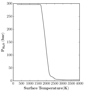
Figure 1: Variation of surface temperature with the outgassed water pressure obtained from Nikolaou et al. (2019) using an interior model coupled with a grey atmospheric model. The thermal emission is obtained for a reasonable range of surface temperature-pressure combinations [$T$,$p$] from this data set using the LBL model.

The initial water inventory chosen by us is slightly more than 1 Earth Ocean (EO$=1.39\times 10^{21}$kg). It is equivalent to 550 ppm or 400 bar. The motivation for this was to investigate the extent by which these starting conditions could reproduce Earth’s ocean reservoir of 300 bar. Using this water inventory, Nikolaou et al. (2019) have obtained the outgassing of water from the mantle using an interior model coupled with a grey atmospheric model, and calculated the variation of surface temperature with the outgassed pressure, denoted as [$T$,$p$] henceforth and shown in Fig. 1. As an assumption, we prescribe their model output as the surface temperature and pressure for our atmosphere model. The range of outgassed pressure during the MO solidification corresponds to $P_{\rm H_{2}O}$ $\sim$ [4, 300] bar (see Fig. 1) which is also the range of the input chosen for the calculation of atmospheric structure and flux of the outgoing longwave radiation, $F_{\rm OLR}$ as explained below.

2.2 Atmospheric structure

In this section, we derive the atmospheric structure for the prescribed surface temperature and pressure as shown in Fig. 1. The atmosphere is assumed to be consisting of only H₂O and is divided into $N=66$ atmospheric layers equally spaced on a logarithmic scale of pressure and calculated by fixing the pressure at the top of the atmosphere to be 1 Pa. The temperature structure of the atmosphere is obtained by assuming a dry adiabatic lapse rate for the atmospheric layers whose temperature is above the critical temperature of water (647 K). Since our calculations begin with a low pressure (4 bar) of water at higher temperatures, therefore, an assumption of the ideal gas equation for the calculation of dry adiabatic lapse is reasonable for our purpose. However, we additionally consider the T-dependence of $C_{p}$ over the whole range of temperatures and pressures. The dry adiabatic lapse rate is calculated from the surface to the top by integrating the equation: $d\ln(T)/d\ln(P)=R/C_{p}(T)$, where $R$ is the gas constant and $C_{p}(T)$ is the specific heat capacity of water with a temperature dependence, which is obtained using the following equation taken from Wagner & Pruß (2002) (and also mentioned by Hamano et al. (2013)):

$$\frac{C_{p}(T)}{R}=1+n_{3}+\sum_{i=4}^{8}n_{i}\frac{(\gamma_{i}\tau)^{2}\exp(-\gamma_{i}\tau)}{[1-\exp(-\gamma_{i}\tau)]^{2}},$$ (2)

where $\tau=T_{\text{c}}/T$ and $T_{\text{c}}$ is the critical temperature (647 K). The value of coefficients $n_{i}$ and $\gamma_{i}$ are taken from Table 6.1 of Wagner & Pruß (2002).

The remaining procedure for calculating the atmospheric structure is the same as the Goldblatt et al. (2013). The tropopause temperature $T_{\rm 0}$ for high surface temperature runs results from the moist adiabatic lapse rate when the pressure at the top of the atmosphere reaches 1 Pa. $T_{\rm 0}$ for our runs ranges from 352 K to 204 K (for decreasing surface temperatures) and it reaches 204 K at $T_{\text{s}}=2900\rm\,K$. For departures from ideal gas behavior, a self-consistent derivation of moist adiabat requires the use of a non-ideal gas equation at high densities (Wordsworth & Pierrehumbert, 2013).

The temperature profiles for the three [$T$,$p$] pairs are shown in Fig. 2. Here, the upper panel illustrates that for a high temperature ($T_{\text{s}}=4000$ K), a dry troposphere is present with no moist layer. However, as the surface temperature decreases ($T_{\text{s}}=1800$ K and $T_{\text{s}}=800$ K; middle panel and lower panel), moist layers of thickness 100 km and 200 km are seen, respectively. The moist upper layers are cooler than the lower layers, hence they act as a cold trap and any exchange of heat from the top of the atmosphere to space becomes less efficient.

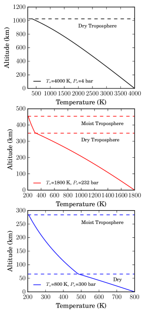
Figure 2: Temperature profiles showing the variation of altitude ($z$) (in km) vs. the temperature of the atmosphere layers for three assumed surface temperatures $T_{\text{s}}$ and associated surface pressure $P_{\text{s}}$ shown in the figure panels and are obtained as an output from the interior outgassing model assuming a grey approach.

2.3 Atmospheric Radiative Transfer

For a gaseous, non-scattering atmospheric assuming local thermodynamic equilibrium, the intensity (radiance) at the Top of the Atmosphere (TOA) is given by the integral of the Schwarzschild equation

$$I(\nu)~{}=~{}I_{\text{b}}(\nu)\,\mathrm{e}^{-\tau_{\mathrm{b}}(\nu)}\;+\;\int\limits_{0}^{\tau_{\mathrm{b}}(\nu)}B(\nu,T(\tau^{\prime}))\;\mathrm{e}^{-\tau^{\prime}}\>\mathrm{d}\tau^{\prime}~{},$$ (3)

where $I_{\text{b}}$ is the background radiation and $B$ is Planck’s function for a black-body with temperature $T$.

The monochromatic transmission $\mathcal{T}$ and optical depth $\tau$ (at position $s=0$, equivalent to $\tau=0$) is a function of wavenumber $\nu$ and path length $s$ and is described by Beer’s law as follows

$$\mathcal{T}\left(\nu,s\right)~{} =~{}\mathrm{e}^{-\tau(\nu,s)}.$$ (4)

In order to solve for the transmission of radiation (Eq. 4), it is important to obtain the optical depth $\tau$ which is written as:

$$\tau(\nu,s)~{}=~{}\int_{0}^{s}\alpha(\nu,s^{\prime})\,\mathrm{d}s^{\prime},$$ (5)

where, $\alpha$ is the absorption coefficient. It is usually written as the sum of the absorption cross sections $\kappa_{m}$ of the molecule, scaled by its number density $n_{m}$ as follows

$$\alpha(\nu,s)~{}=~{}\sum_{m}\kappa_{m}\bigl{(}\nu,p(s),T(s)\bigr{)}\,n_{m}(s).$$ (6)

For high resolution lbl models, the absorption cross section of molecule $m$ is given by the superposition of many absorption lines $l$, each described by the product of a temperature-dependent line strength $S_{l}$ and a normalized shape function $g$ describing the broadening mechanism. The calculation for the absorption coefficient and the absorption cross section for the molecules is described in the next section.

Assuming the net energy balance of the incoming and outgoing radiation at TOA, along with the cooling flux from the magma ocean, one can write

$$F_{\rm OLR}-F_{\rm SUN}=F_{\rm MAG}.$$ (7)

Here, $F_{\rm OLR}$ is the flux of the outgoing longwave radiation calculated using GARLIC at a viewing angle of 38^∘ from zenith (See Sect. 3 and Appendix A) and $F_{\rm SUN}=(1-\alpha)S_{0}/4$, where $S_{0}$ is the solar constant with 100% luminosity and a fixed surface albedo of $a=0.3$ is used. For simplicity, we do not include the effect of clouds and Rayleigh scattering.

2.4 GARLIC

The “Generic Atmospheric Radiation Line-By-line (lbl) Infrared Code” or finds its applications in several fields such as exoplanet studies (Rauer et al., 2011; Hedelt et al., 2013; Vasquez et al., 2013a, b) and for Venus type atmospheres (Hedelt et al., 2011; Vasquez et al., 2013c). GARLIC has been recently used to study Earth’s atmosphere (Hochstaffl et al., 2018; Xu et al., 2018) for retrieval purposes in the field of remote sensing. Moreover GARLIC has been validated using the transmission spectroscopic studies involving ACE-FTS infrared observations of the Earth (Schreier et al., 2018a). Furthermore, an inter-comparison of radiance obtained from the three lbl models: GARLIC, KOPRA and ARTS in 18 channels throughout the mid-IR is presented in Schreier et al. (2018b).

In this work, the line absorption coefficients for molecule H₂O and other species are calculated by GARLIC using the 2010 HITEMP line list, i.e., the high temperature molecular spectroscopic database by Rothman et al. (2010) and a “CKD continuum” model (Clough et al., 1989) for H₂O. The latest spectral database HITRAN 2016 (Gordon et al., 2017) is also used towards the end for comparison. A Voigt profile (Schreier et al., 2014), representing the combined effect of pressure broadening together with Doppler broadening is used.

The high resolution spectra in GARLIC are obtained by construction, i.e., the wavenumber grid spacing is adjusted to the line widths $\delta\nu=\gamma/n$, where $n$ is by default 4 and $\gamma$ is the half width half maximum (HWHM) dependent on the pressure, temperature, and molecular mass. Since the Lorentz width is proportional to the pressure, lines become narrower in the upper atmosphere. In GARLIC, the final grid (i.e. for all layers and molecules combined) is defined by the smallest $\delta\nu$.

We have verified the GARLIC code for a pure steam atmosphere at small temperature of $T=300$ K with a background surface pressure of 1 bar with the published results of Goldblatt et al. (2013) and Schaefer et al. (2016).

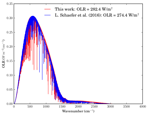
Figure 3: Comparison of emitted radiance as a function of frequency (0-3500 cm^-1) for a pure H₂O atmosphere at $T_{\text{s}}=300$ K and $P_{\text{s}}=1$ bar using the LBL code GARLIC.

A spectrally averaged OLR of 282.4 W/m² is obtained which is close to the result of Schaefer et al. (2016), i.e., 274.4 W/m² as seen in Fig. 3. Also it is in a good agreement with Goldblatt et al. (2013) who obtained 282 W/m² for modern Earth using the LBL code SMART (Meadows et al., 1996).

At high surface temperatures and pressures and for a fixed tropopause temperature of 344 K, we compared the OLR values with the former studies using lbl codes. The comparison is presented in Table 2. The values are comparable for $T_{\text{s}}=1000$ K but for higher temperature $T_{\text{s}}=2000$ K, there seems to be a large deviation. The difference at high surface temperatures is attributed to the choice of the water continuum and due to the fact that the continuum is poorly understood at high temperatures.

Table 2: Comparison of OLR for high temperature runs calculated using GARLIC with the former lbl studies.

$T_{0}$	$T_{s}$	$P_{s}$	OLR
(K)	(K)	(bar)	(W/m2)
344	1000	100		795.9b	801.4c
344	1000	250	789a		784.54c
344	2000	250	969a		1400c

• Goldblatt et al. (2013)

• Schaefer et al. (2016)

• This study

2.5 Effective height

The effective height of the atmosphere, which is a function of the wavenumber describes the extent of the atmosphere and is directly measured from the transit observations. For calculating the effective height from the transmission spectra, we use the following equation

$$h(\nu)=\int_{0}^{\infty}\left(1-\mathcal{T}(\nu,z_{i})\right)dz_{i},$$ (8)

where the integral is calculated over all the limb transmission spectra with tangent altitude $z_{i}$ for every incident ray $i$ passing through the atmosphere terminating at the TOA. For more details, see Schreier et al. (2018a).

2.6 Chemical equilibrium with applications (CEA)

At $T_{\text{s}}>2000$ K, water is expected to undergo thermal dissociation leading to a somewhat different composition of the atmosphere that may influence the OLR and thereby the MO lifetime. Therefore, we employ the NASA CEA (Chemical Equilibrium with Applications) model to calculate the chemical equilibrium compositions and properties of various species formed as a result of the thermal dissociation of water at such high temperatures. The CEA calculates the chemical equilibrium concentrations of species from any set of initial composition(s) for a given [$T$,$p$]. Some of the built-in applications of the program include calculation of theoretical rocket performance, Chapman-Jouguet detonation parameters, shock tube parameters, and combustion properties (B. J. McBride et al., 2002; Snyder, 2016). The CEA program utilizes a Gibbs free energy minimization routine to obtain the equilibrium-state composition for a given [$T$,$p$]. The thermodynamic data for the species are obtained from the NASA CEA database (Snyder, 2016).

The scale height of the atmosphere also depends on the composition as the atmosphere and is calculated using the same procedure as described in Sect. 2.2 but with an updated mean molecular weight $\mu^{*}=f_{\rm H_{2}O}\,\mu_{\rm H_{2}O}+f_{\rm H}\,\mu_{\rm H}+f_{\rm H_{2}}\,\mu_{\rm H_{2}}+f_{\rm O}\,\mu_{\rm O}+f_{\rm O_{2}}\,\mu_{\rm O_{2}}+f_{\rm OH}\,\mu_{\rm OH}$, where the additional species are formed as a result of thermal dissociation of water.

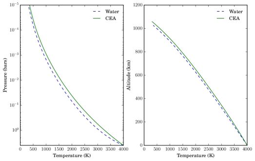
Figure 4: Temperature profiles (a) showing the variation of pressure with temperature of the atmosphere layers consisting of pure water atmosphere vs. CEA for a fixed surface temperature of 4000 K and a pressure of 4 bar (b) altitude (z) (in km) with the temperature for pure water and CEA.

Fig. 4 shows a comparison between the temperature profiles of water and the CEA composition for a surface temperature of 4000 K and a surface pressure of 4 bar. Only a minor difference in the scale height is observed while comparing CEA composition with water. Also, the effect of the CEA composition on the OLR is small and is discussed later in Section 6.

2.7 Framework

The detailed framework of the paper is as follows. First of all, the atmospheric temperature profiles (as illustrated in Fig. 2) are pre-calculated for a range of surface temperatures $T_{\text{s}}$ = 800 to 4000 K, sampled at a resolution of $\Delta T_{\text{s}}=100$ K (from 800 K - 1400 K and 1900 K - 4000 K) and a higher resolution of $\Delta T_{\text{s}}=\rm\,20K$ (1420 - 1800 K). For the surface pressure range between 4 and 300 bar, the values 4, 25, 50, 100, 150, 200 and 300 bar are chosen. In total, we calculate temperature profiles for pairs of [$T$,$p$] lying on a grid of 400 points. Then, using the temperature profiles of these 400 [$T$,$p$] points as input, $F_{\rm OLR}$ is calculated for a 100% H₂O atmosphere using the LBL code GARLIC.

Secondly, the resultant $F_{\rm OLR}$ is used complimentarily to a range of MO thermal evolution experiments performed with the interior model in Nikolaou et al. (2019). The time evolution of surface temperature is a coupled result reported in both the studies. However, in this study, we focus on assessing the spectral evolution of the pure steam atmosphere.

Thirdly, we obtain the outgoing longwave radiation for a special case involving thermal dissociation of H₂O using the CEA model. The influence of equilibrium chemistry upon the radiative spectra is also discussed.

3 Thermal emission

The planetary thermal emission is obtained for 400 [$T$,$p$] points as described in the Sect. 2.7. These are calculated using the LBL code GARLIC for a down-looking observer at a viewing angle of 38^∘ with the zenith angle as also chosen by Segura et al. (2003); Rauer et al. (2011) and Grenfell et al. (2011). This angle is considered to be the “mean angle” or “equivalent latitude” at which the solar insolation incident upon Earth is 341 W/m² which is equal to one quarter of the present solar constant $S_{0}=1361$ W/m². The solar radiation, $F_{\rm SUN}$ in our model is taken to be one quarter of $S_{0}(1-\alpha)$ which justifies the OLR calculation at 38^∘ viewing angle.

Figure 5: Emission spectra as a function of wavelength ranging from the visible to the infrared for four different [$T$,$p$] cases. The corresponding Blackbody (BB) curves for each of these surface temperatures (in blue) and the flux at effective radiating temperature (dotted line) are shown.

The flux (integral of radiance over the solid angle) in the units of $\rm\,W/m^{2}\mu m^{-1}$ at each [$T$,$p$] as a function of wavelength (ranging from mid UV to infrared) is shown in Fig. 5 for a 100% steam atmospheres and for four [$T$,$p$] pairs. The effective radiating temperature defined as, $T_{\rm rad}=\sqrt[4]{F_{\rm OLR}/\sigma}$ is obtained, where $F_{\rm OLR}$ is calculated by integrating the flux over 5000 points of wavenumber. Using Planck’s law, the electromagnetic flux corresponding to $T_{\rm rad}$ at the radiative emitting (top) layer is shown in Fig. 5 (dashed line).

For a [$T$,$p$] pair with high temperature ($T_{\text{s}}=4000$ K) and low pressure ($P_{\text{s}}$ = 4 bar) as in the uppermost panel of Fig. 5, the peak of the maximum emission is at small wavelength (following Wien’s displacement law). Hence the radiation can escape through the window regions at small wavelengths. At lower surface temperatures (lower panels), the amount of water vapour in the atmosphere increases (because of increased outgassing), leading to a decrease in the emitted flux. Also, the peak of the emission moves towards longer wavelength (following Wien’s displacement law), where radiation is effectively absorbed by the atmosphere. Due to this, the spectroscopic window region becomes optically thick, e.g., at 1$\rm\mu m$. As a consequence, the radiation drops by $\sim$ 10 orders of magnitude from the uppermost panel (4000 K, 4 bar) to the lowermost panel (800 K, 300 bar).

A comparison between the effective radiative temperature and the surface temperature of early Earth for variable outgassing and a fixed surface pressure of 300 bar [e.g. Kasting (1988); Marcq (2012); Marcq et al. (2017)] is shown in Fig. 6.

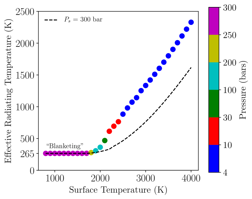
Figure 6: Variation of effective radiating temperature vs. the surface temperature with variable outgassing pressure and a fixed surface pressure. The effective radiating temperature is found to be lower for the latter case. The pressure variation is shown as the color bar. The runaway greenhouse limit is obtained for surface temperatures below 1800 K, as the surface is blanketed by water vapour. A fixed effective radiative temperature of 265 K is obtained.

We notice here that the effective radiating temperature $T_{\rm rad}$ is less than the surface temperature, $T_{\text{s}}$. This is because of the greenhouse effect of water. Since we take into account a variable outgassing ranging between 4- 300 bar of water, the effective radiative temperature in the range $265<T_{\rm rad}<2300$ K are higher as compared to the fixed surface pressure (300 bar) where the range is much smaller, i.e. $265<T_{\rm rad}<\rm\,1600K$. For example, Marcq (2012) obtained an effective temperature of 350-400 K for $T_{\text{s}}=2350$ K for a fixed water pressure of $\sim$ 300 bar, whereas we obtain an effective temperature of 600-700 K by considering variable pressure. In the latter case, an efficient cooling of the planet is expected. A “blanketing effect”, i.e., obscuring of the surface due to steam lying in the atmosphere begins at $\sim 1800$ K. For $T_{\text{s}}<1800$ K, the planet is effectively radiating at $T_{\rm rad}=265$ K and a fixed OLR of $282\rm\,W/m^{2}$. This means that the top of the atmosphere’s thermal spectrum is bounded by the flux from effective radiation temperature of 265 K in this region.

Using the OLR calculated for the 400 grid points of [$T$,$p$], a bilinearly interpolated grid is calculated (Nikolaou et al., 2019) to facilitate an effective coupling of the atmospheric model with the interior model within a continuous range of outgassed pressures [4,300] bar as a function of $T_{\text{s}}$ [800,4000] K, based on the actual [$T$,$p$] output of the interior model.

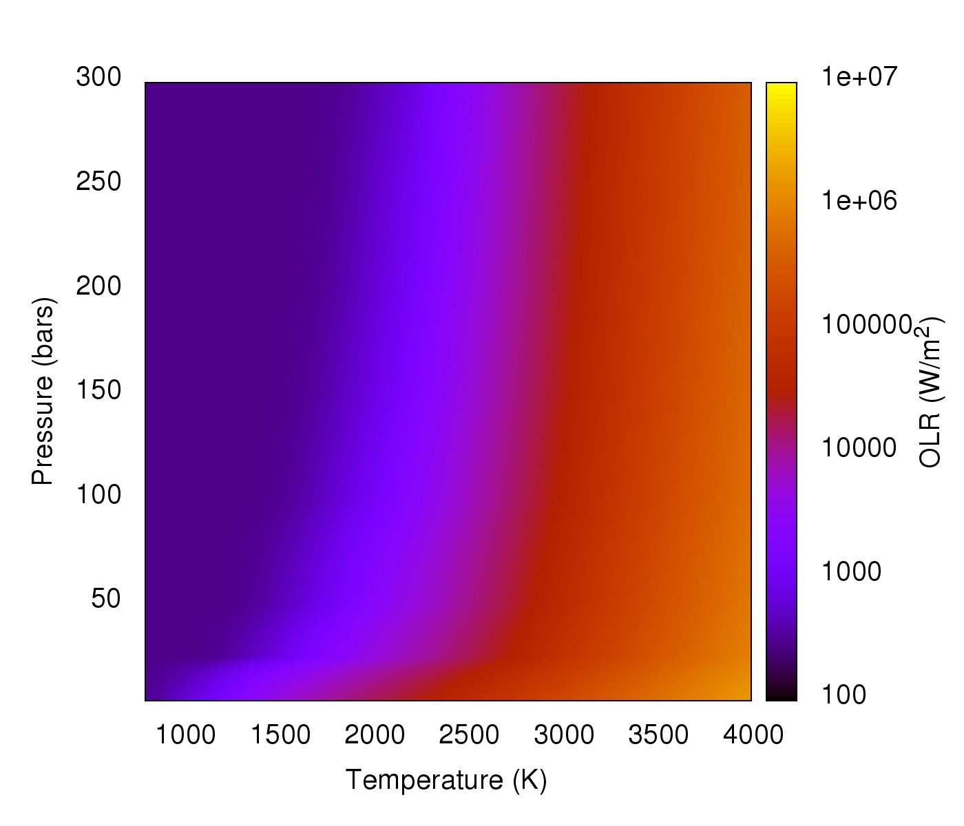
Figure 7: Result of bilinear interpolation from fixed $[T,p]$ grid of 400 points onto a new grid which then serves as an input to the interior model in order to obtain the MO thermal evolution.

The output of the interpolation is shown in Fig. 7. We then investigate the coupled interaction of the interior and atmosphere in the next Section 4.

4 Coupled Atmosphere-Interior model results

The calculation for the MO evolutionary model (described in detail in Nikolaou et al. (2019)) begins at a very high surface temperature of 4000 K, which corresponds to a molten state of the full mantle. The time period of formation of Earth is assumed to be 100 Myrs. Therefore, to account for the calculation of the onset of thermal cooling of the mantle, 100 Myrs is subtracted from the time of evolution in our model.

By assuming a radiation balance at top of the atmosphere, an iterative loop (starting at an initial time step) with a convergence criteria $\epsilon$ is run until the following fluxes are equal, meaning they numerically converge to the same value:

$$|[F_{\rm OLR}(T,p)-F_{\rm SUN}]-F_{\rm MAG}|<\epsilon,$$ (9)

where $\epsilon=0.1$ W/m² is equal to the uncertainty in the OLR values obtained by using GARLIC. Once the iterative loop in Eq. (9) is satisfied at a particular time step, the surface temperature $T_{\text{s}}$ is then obtained and a new potential mantle temperature $T_{\text{p}}$ is calculated at the next time step by using the MO evolutionary model (described in detail in the companion paper). If Eq. (9) is not satisfied, the surface temperature is adjusted by a factor $\Delta T_{\text{s}}$ and the corresponding $F_{\rm OLR}$ is chosen from the interpolated grid (see Fig. 7) and F_MAG is re-calculated. The steps are repeated until the surface temperature reaches approximately 1650 K (i.e., $T_{\rm RF,0}$), as mentioned before. Therefore, the calculations for the MO evolutionary model have been carried out until $T_{\text{s}}\sim 1650$ K. Note that this value is different from the $T_{\rm RF,0}$ of Hamano et al. (2013), i.e., $\sim 1370\rm\,K$ due to different assumptions in their rheology front. We do not perform calculations for the case of a warming planet, i.e., when a negative left hand side in Eq. (9) is obtained. The case for the latter is designated as planet type II by Hamano et al. (2013).

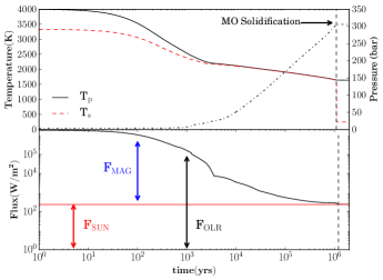
Figure 8: Upper Panel: Variation of the surface temperature $T_{\text{s}}$ and the potential mantle temperature $T_{\text{p}}$ as a function of time as obtained by Nikolaou et al. (2019). MO solidification (vertical dashed line) is obtained at $\sim$ 1 Myr. Evolution of surface pressure (dot-dashed line) as a measure of outgassing is also shown on the right axis. Lower panel: Variation of the energy fluxes: flux from the emitted radiation F_OLR (black), solar incoming flux F_SUN (red) and flux from magma ocean $F_{\rm MAG}$ (blue) are shown.

The time evolution of $T_{\text{s}}$ is shown in Fig. 8. As seen in the upper panel of Fig. 8, initially both potential temperature $T_{\text{p}}$ and the surface temperature $T_{\text{s}}$ start to cool efficiently but at different rates, and reach $T_{\text{s}}$ $\sim 2150$ K after 0.25 $\times$ 10⁴ yrs. Thereafter, cooling slows down because the atmosphere starts to limit the escape of heat flux from the interior. This is evident from the rise of outgassed steam pressure as seen towards the right of the upper panel of the figure. It can be clearly seen that the outgassed steam pressure rises from 4 bar to about 300 bar during the evolutionary phase of the MO. Finally, the MO solidification is achieved at $\sim 1\rm\,Myr$. This is similar to the time obtained by Hamano et al. (2013) when they set the surface solidification temperature of $T_{\text{R}F,0}\sim 1700\rm\,K$, close to our value of 1650 K.

Furthermore, in the lower panel of Fig. 8, it is seen that $F_{\rm OLR}$ approaches the radiation limit of $\sim 282\rm\,Wm^{-2}$ only by the end of the MO phase. A reduction in the $F_{\rm MAG}$ (=$F_{\rm OLR}$-$F_{\rm SUN}$) with time indicates thermal cooling of the magma ocean.

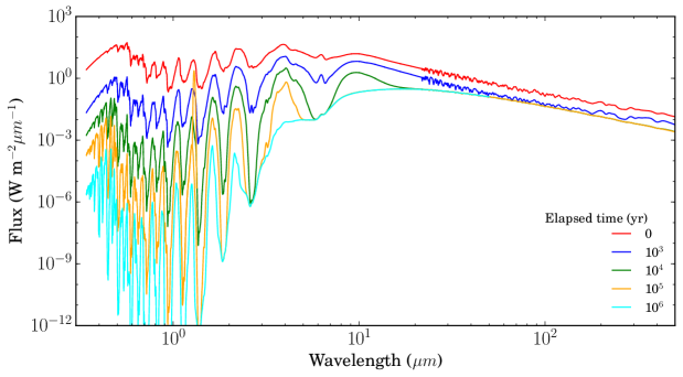
Figure 9: Evolution of the thermal spectra in the visible and IR during the solidification of the magma ocean which outgasses $\sim$ 300 bars of water into the atmosphere. The spectra are shown for the entire wavelength regime 0.34-200 $\rm\mu m$ considered for the study. The color of the emission spectra indicates the elapsed time after the MO solidification starts. The thermal emission is seen to be constant for later times at IR wavelengths indicating that the emission has reached a radiation limit.

Fig. 9 shows the spectral response of the thermal emission for different times elapsed during MO evolution. For smaller timescales in early evolutionary stages (i.e., red solid line), due to high surface temperature and less surface pressure of water vapour in the atmosphere, the thermal radiation is quite high and escapes to space efficiently. However, these thermal fluxes rapidly decrease with time due to the decrease in the surface temperature and an increasing surface pressure at later times $\sim 10^{3}-10^{4}$ yr. This leads to an increased optical thickness of the atmosphere (due to water outgassing) and a ‘closing’ of the associated IR absorption window.

As illustrated in this figure, thermal fluxes at later times $\sim 10^{4}-10^{6}\rm\,yr$ tend to become constant for $\lambda>10\rm\,\mu m$ which implies that the steam atmosphere is lying in the radiation limit. This is also evident from the lower panel of Fig. 8, where $F_{\rm OLR}$ is seen to become constant at a value of $282\rm\,Wm^{-2}$ (OLR limit).

The largest contribution to the emission spectra of the hottest scenarios is from the shorter wavelengths (U band) because of the absence of strong water absorption lines. In this case, a detailed diagnostic measure of a planet’s atmosphere can be obtained from its thermal emission as seen in the visible and near-IR wavelengths, i.e. M, L, Ks band (e.g. water absorption bands in the $1-8\rm\mu m$ region). With the decrease in $T_{\text{s}}$ and growth of the steam atmosphere, U band’s contribution to the OLR decreases with time whereas the bands M, L, Ks initially decrease and then become constant with time indicating that the OLR limit has been reached.

Notably, the spectral band feature at $\sim 6.3\rm\,\mu m$ in Fig. 9, related to the absorption by water vapour in the atmosphere is seen to broaden (because of pressure broadening) with the increase of the amount of outgassed steam suggesting that the atmosphere is saturated with water.

5 Observables

5.1 Transmission spectra

Transmission spectroscopy is a widely-used tool to constrain the composition of planetary atmospheres. For exo-planetary studies, it has been recently used in this way to provide the first hints on bulk atmospheric composition and clouds of Earth-size planets, for example Trappist-1b and c (Wit et al., 2016), water bands in Neptune-sized exo-planets HAT-P11b (Fraine et al., 2014) and HAT-P-26b (Wakeford et al., 2017) and H₂ rich atmosphere of planet GJ3470b (Ehrenreich et al., 2014).

Using our 1D atmospheres and the radiative transfer code, we calculated the transmission spectrum ranging from 0.34-30$\rm\mu m$. It is shown as the wavelength dependent effective height in Fig. 10 for the whole duration of the magma ocean. The spectra are computed at a very high resolution as explained in Sect. 2.4 using the HITEMP2010 database, and then binned to a resolution of $\lambda/\Delta\lambda=1000$. As the magma ocean solidifies over time with the decrease in the surface temperature (see Fig. 8), the effective height of the atmosphere is reduced. Note that the abundance of water molecules for different elapsed time of the magma ocean is the same. The depth of the atmosphere where the absorption by the water vapor takes place is found to be $\sim$ 100 km, in contrast to 10-20 km for modern Earth (Wunderlich et al., 2018).

As a comparison, the results of the effective height using the latest database HITRAN2016 (Gordon et al., 2017) are presented in Fig. 11. The variation in the absorption features in the two cases is due to the fact that HITEMP2010 consists of many more molecular bands and line transitions at high temperatures. HITRAN2016 (Gordon et al., 2017), on the other hand, has an expanded database of water vapor as compared to the previous HITRAN versions. The difference in the two databases is appreciable at high temperatures and low pressures and looks same $T_{s}<2100$ K as illustrated in the Appendix B.

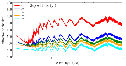
Figure 10: The effective height of the atmosphere as a function of wavelength for the whole duration of magma ocean using HITEMP10 database. The effective height of the atmosphere is seen to reduce as the magma ocean solidifies.

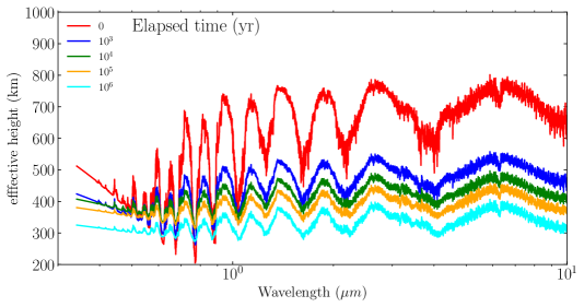
Figure 11: Same as above figure but with the latest HITRAN16 database.

6 Chemical equilibrium Analysis

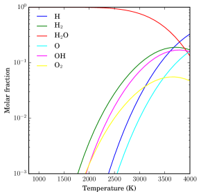
Figure 12: Mole fraction as a function of temperature at pressure of 4 bar for various species formed as a result of water dissociation calculated using the NASA CEA program.

For the early stages of the MO, it can be expected that due to thermal dissociation of H₂O at $T_{\text{s}}>\rm\,2000K$, additional species such as H, O, O₂, O, and OH are formed. The molar fraction of these species as a function of temperature is shown in Fig. 12. For this example, we set $P_{\text{s}}=4$ bar (corresponding to $T_{\text{s}}=4000\rm\,K$ as per the interior outgassing model). It can be seen that at $T_{\text{s}}=4000$ K, only 13% H₂O is present and the rest is dissociated into H (32.9%), H₂ (17%), O (16%), OH (15%), O₂ (4.7%), and other trace elements. Moving to lower temperatures, the molar fraction of the other species reduces and water constitutes 100 % at $T_{\text{s}}\sim 2000\rm\,K$. Note there is a peak in H₂ and O₂ fractions at temperatures around $3500-4000\rm\,K$. This is potentially relevant for assessing O₂ false positives in atmospheric biosignature science.

The molar fraction as a function of temperature obtained using the NASA CEA program are verified with another equilibrium chemistry codes, e.g. (personal communication, L. Schaefer) which is also used in Schaefer et al. (2004) and recently in Schaefer et al. (2017).

The higher the atmosphere, there are more chances to detect it through the pioneering transit observations. Hence, a planet in early stages of magma ocean would have perhaps more chances of detection through charaterization of its composition.

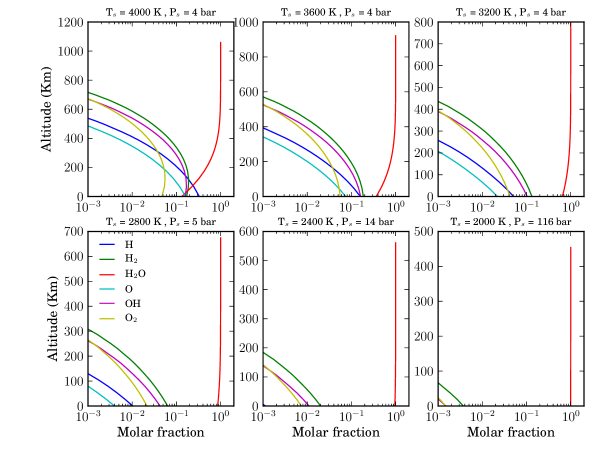
Figure 13: Altitude vs. molar fraction for various species for various surface temperatures and surface pressures as indicated on top of each panel (following interior outgassing rates). This plot shows height profile of various species in the atmosphere as a result of thermal dissociation of water.

Atmospheric concentration profiles (altitude vs. molar fraction) for various species and temperature-pressure combinations are shown in Fig. 13. The surface temperature and pressure are according to the outgassing rates of the interior, as mentioned on the top of each panel in this figure. It is to be noted that the initial concentration of H₂O is set by the outgassing and is therefore dependent on the surface temperature.

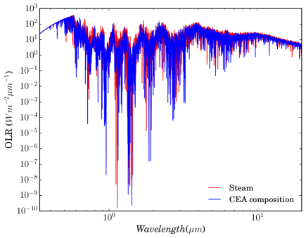
Figure 14: Comparison of OLR for 100% steam atmosphere vs. CEA composition atmosphere where the effect of thermal dissociation of H₂O is included (see text) for a case with $T_{\text{s}}=4000$ K and $P_{\text{s}}=4$ bar.

Figure 14 shows a comparison between the emission thermal spectra or OLR as a function of wavelength for a 100 % steam vs. the equilibrium chemistry composition (obtained using CEA) for $T_{\text{s}}=4000$ K and $P_{\text{s}}=4$ bar. The OLR for the CEA composition is found to be lower by 5-6% than the pure steam case. The species which dominate the CEA composition namely, H₂ and H might be responsible for lowering the OLR. However, the O bearing species, namely O₂, OH and O did not result in any change in the OLR value. The impact of CEA on the MO solidifcation time is hence expected to be negligible. More discussion related to absorption by H₂ is presented in Sect. 7.3.

We also compare the effective height of an atmosphere constituting pure water vs. the individual species of the CEA profile at $T_{\text{s}}=4000\rm\,K$ and $P_{\text{s}}=4$ bar using HITRAN16 spectral database as shown in Fig. 15. The lowered fraction of H₂O in CEA case results in a slightly higher effective height (cyan line) as compared with 100% abundance of H₂O (orange line) according to the equation $H=kT/\mu g$. Due to the thermal dissociation of water at higher temperatures, O and H bearing species contribute a significant amount to the effective height of the atmosphere. Different absorption behavior with altitude leads to spectral features arising at different altitudes as seen in Fig. 15. One can see strong absorption features for the species, namely for H₂O, H₂, O₂ but the contribution of each species towards the transmission as a whole is not linearly additive. Due to this property, the effective height of the atmosphere for the CEA profile with all the species (red line) is seen to be overlapping with the CEA profile when considering only water as absorber in the lbl calculations in cyan. The difference in the spectra of H₂O of CEA profile (cyan line) and spectra of pure H₂O atmospheres (orange line) is mainly due to the increase in the scale height of the atmosphere, so the overall effective height increases.

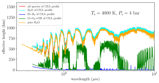
Figure 15: Comparison of effective height of the atmosphere for pure water vs. individual speciation for the CEA profile using spectral database HITRAN16.

7 Discussion

One of the key objectives of the paper was to study the thermal spectral evolution of the early Earth, i.e. during the MO phase using a line-by-line atmospheric model. We have performed a systematic study of the spectral evolution for a steam based atmosphere by including the time-dependent outgassing rates obtained from Nikolaou et al. (2019). We briefly summarize and discuss our results below.

7.1 Model Comparison

The model employed in this study has some strengths and simplifications over others. For the calculation of the thermal emission using GARLIC, we solve the radiative transfer in the spectral range 20-29,995 cm^-1 ($\sim$ 0.333- 500 $\rm\mu m$), while Goldblatt et al. (2013) have evaluated in the range of 50-100,000 cm^-1 (0.1-200 $\rm\mu m$) for a combined thermal and solar radiation calculation. For the latter, the absorption in the 0.2-0.33 $\rm\mu m$ regime is derived by using Rayleigh scattering as no LBL cross sections are available. For our purpose, we calculate only the thermal part using GARLIC with HITEMP2010 as the spectral database. The appendix provides a comparison between HITEMP2010 and HITRAN2012 (Rothman et al., 2013). The far-wing absorption by water vapour is a strong function of the continuum. We use a CKD approach (Clough et al., 1989) as compared to MTCKD2.5 used by Goldblatt et al. (2013), Hamano et al. (2013, 2015). It is to be noted that Schreier et al. (2018a) found the results with CKD to be almost comparable to the one obtained using MTCKD2.5.

The specific heat capacity of water vapour has a temperature dependence. We use empirically formulated $C_{p}(T)$ provided by Wagner & Pruß (2002) instead of using steam tables as done by Kasting (1988); Goldblatt et al. (2013); Marcq et al. (2017) and Schaefer et al. (2016). The latter have used the steam tables by Lide (2000).

Most of the magma ocean models (Elkins-Tanton, 2008; Lebrun et al., 2013; Marcq et al., 2017) have considered the effect of CO₂ along with H₂O as an important greenhouse atmospheric component. We have included only H₂O and do not include CO₂ in order to simplify the calculations for the atmospheric structure. Also, at high temperatures, there is a possibility of CO₂ getting dissociated to C and O₂, and both of them being sequested back to the mantle (Hirshmann, 2012; Schaefer et al., 2016) causing the oxygen fugacity to increase. Such scenarios are hence important for outgassing by secondary volcanism during a post-magma ocean state (e.g. Tosi et al., 2017).

A major strength of our atmospheric model is that it treats different amounts of H₂O outgassed from the interior as a function of surface temperature as compared to Marcq et al. (2017) who assumed a fixed outgassing steam pressure of 270 bar. Hence, our atmospheric model is physically more consistent with input from the interior, i.e outgassing rates as a function of varying surface temperature.

On the other hand, our model predicts a higher OLR as a function of surface temperature as compared to the OLR values of Hamano et al. (2015) at fixed surface pressure. A difference of two orders of magnitude between our OLR values with the one presented in Figure 5 of Ikoma et al. (2018) are partly due to the non-inclusion of Rayleigh scattering process and the choice of water vapor continuum (i.e. CKD). When we included the Rayleigh scattering, this led to comparable results for fixed surface pressures as Fig. 5 of Ikoma et al. (2018) and Goldblatt et al. (2013) for a pure water vapour atmosphere. An illustration of differences in the OLR values using several different radiative transfer codes for steam-based atmospheres is presented in Yang et al. (2016).

Furthermore, since Marcq et al. (2017) have included spectral wavelength longward of 1 $\rm\mu m$ only for the calculation, they might be underestimating the OLR values for $T_{\text{s}}>2400\rm\,K$, wherein most of the absorption happens at wavelength shortward of 1 $\rm\mu m$. Therefore, in our study, we have extended the shortwave calculations up to $0.34\rm\,\mu m$ (29,445 cm^-1). As a result, we find that the component of OLR shortward of $1\rm\,\mu m$ has an important contribution, i.e. it contributes $\sim$ 1.2% of the total OLR for $T_{\text{s}}=1800\rm\,K$; 38% for $T_{\text{s}}=2500$ K and $\sim 90$% for $T_{\text{s}}=4000\rm\,K$. This suggests it is important to include a radiation contribution shortward of $1\rm\,\mu m$ to account for the absorption of thermal radiation and outgoing longwave radiation at high surface temperatures (e.g., $T_{\text{s}}>2400$ K).

In this paper, we have not included atmospheric escape of hydrogen and oxygen as illustrated by e.g., Schaefer et al. (2016, 2017) but we included the thermal dissociation of water at higher temperatures leading to the formation of additional species such as H, H₂, O, O₂, and OH in chemical equilibrium with each other. Out of these, H₂ could act as a greenhouse gas which is lying in the lower parts of the atmosphere. This results in lowering of the OLR by causing more absorption of radiation in the infrared spectral regime. In addition, H₂O may get photolysed, which may lead to a further change in composition of the atmosphere.

Hamano et al. (2013) have found a significant water loss of type II planet during the magma-ocean period which lasted around about 100 million years (long-term MO). They have also suggested a strong escape of H-atoms to space while O₂ would be dissolved in the MO. The latter is believed to increase the oxygen fugacity of the mantle by up to about 0.07 wt%. Therefore, the photolysis and H escape, both are significant processes that impact the atmospheric composition and mass, for e.g. it is also shown by Schaefer et al. (2016) that H escape leads to the build up of O₂. The planet GJ1132b studied by Schaefer et al. (2016) is in a long term MO, so H escape is a significant process in order to loose more water quickly. In contrast, for a short duration MO planet studied by us, we only studied the process of thermal dissociation of water which leads to a H₂-dominated lower atmosphere along with some abiotic production of O₂ during the onset of the MO. This corroborates with the findings for the case of exoplanet GJ1132b by Schaefer et al. (2016) and recently for the two innermost TRAPPIST planets- TRAPPIST-1b,1c (Schaefer et al., 2017), that employed chemistry calculations along with diffusion.

7.2 MO solidification times

The initial content of H₂O inside the mantle is assumed to be low, i.e., 5.5 $\times$ 10^-2 wt % in this study. Using this, we find that the melt fraction at the surface reaches the critical value of 0.4 at a temperature $T_{\text{s}}=1650$ K, marking the end of the magma ocean where the entire mantle exhibits a solid-like behavior (e.g. Nikolaou et al., 2019). Hence, the mantle cools down via solid-state convection much more slowly than via liquid-like convection, which characterizes the magma ocean phase. We estimate the solidification time of the MO at this surface temperature to be $\sim 1\rm\,Myr$. Hamano et al. (2013) have obtained the duration of magma ocean to be $\sim 4\rm\,Myrs$ for a surface solidus temperature of $T_{\rm s}=1370\rm\,K$ (using a different rheology front) and for an increased initial water inventory (5 $M_{\rm EO}$). However, their estimate becomes quite close to our findings upon setting their solidification temperature to $T_{\text{s}}=1700\rm\,K$ (close to our value of 1650 K) in which case the lifetime of magma ocean reduces to $1\rm\,Myr$ (see also discussion in Nikolaou et al. (2019)).

Furthermore, upon using the original setup of the Marcq (2012) atmospheric model, the duration of MO solidification is reported to be $\sim$ $1\rm\,Myr$ in Lebrun et al. (2013). However, the updated model version of Marcq et al. (2017) obtained a 2.5 times reduction in this value, i.e.to $8.0\times 10^{5}\rm\,yrs$ for a H₂O-CO₂ dominated atmosphere, and for a slightly smaller initial water inventory, i.e. $4.3\times 10^{-2}\rm\,wt\%$. On the other hand, a higher initial H₂O inventory of 100 Earth oceans used by Schaefer et al. (2016) is able to extend the MO lifetime to $\sim 8\rm\,Myr$ due to enhanced outgassing. Hence, the solidification timescales are very sensitive to the initial water inventory used. These along with the other factors affecting the MO solidification times are discussed in detail by Nikolaou et al. (2019).

Our results of MO solidification timescale compare well with the existing 1D radiative-convective model studies presented by Hamano et al. (2013, 2015) and Marcq et al. (2017) for similar parameters. In Table 3, we provide a list of various coupled atmospheric-interior models in the literature and present a comparison of their results with our study.

Table 3: A comparison table for the MO cooling timescales for various coupled atmospheric-interior models. The MO cooling timescales are mentioned in the last column with the type of planet I or II and the water inventory in the parentheses.

Reference	Rad. transfer	Initial water inventory	Solidification	MO cooling timescale
	method	MEO & (wt %)	temperature (K)	(Myr)
Lebrun et al. (2013)	correlated-$k$	1	1,400	1 (Planet Earth)
	(grey)	(4.3$\times$ 10-2)
Hamano et al. (2013)	correlated-$k$	0.01-10	1,370	4 (Type I; 5 MEO)
	(grey)	31,370	100 (Type II)
Hamano et al. (2015)	correlated-$k$	0.01-50	1,370	3.9 (Type I; 5 MEO)
	(non-grey)	(2.3$\times$ 10-4-1.2)	1,370	100 (Type II; 5 MEO)
			1,700	1 (Type I)
Schaefer et al. (2016)	LBL	0.1-1000	1,420	8 (100 MEO)
	(non-grey)	(up to 20)
Marcq et al. (2017)	correlated-$k$	1	1400-1,650	0.8
		(4.3 $\times$ 10-2)
This study (2018)	LBL GARLIC	1	1,650	1
	(non-grey)	(5.5 $\times$ 10-2)

7.3 H₂ as greenhouse gas

H₂ has been discussed as an important infrared absorber and radiative gas by e.g., Pierrehumbert & Gaidos (2011) and Wordsworth (2012) who suggested warming of the Martian surface due to an enhanced H₂ greenhouse effect for at least a few tens of Myr. Using a 1-D climate model for early Mars with a surface temperature of 273 K and pressure of 2 bar, Ramirez et al. (2014) have obtained a reduction in the OLR by 6 and $22\rm\,Wm^{-2}$ due to the increase in the H₂ abundance by 5 and 20%, respectively.

Diatomic H₂ interacts with the radiation via collision-induced absorption (CIA), absorbing strongly in the middle and lower portions of the atmosphere and causing it to be a potential contributor to greenhouse warming during the early Earth (Wordsworth & Pierrehumbert, 2013). Moreover, CIA by H₂-H₂ is known to dominate the radiative transfer of heat in the atmosphere of early Earth and other major planets. For example, a study by McKay et al. (1991) shows H₂ as one of the key absorber of radiation in the Titan’s infrared spectrum and hence responsible for its greenhouse effect.

Our results on the thermal dissociation of steam using chemical equilibrium runs suggest a small build-up of O bearing species: O₂, OH, and O. On the other hand, a significant fraction of H (32.9%) and H₂ (17%) is found for the case with surface temperature of $T_{\text{s}}=4000$ K (i.e. at the onset of MO solidification). The concentration of these newly formed species, however, decreases as the temperature decreases. Looking at the atmospheric concentration profiles (Fig. 13), we see that the newly formed species with a molar fraction $>10^{-2}$ are lying at altitude less than 600 km in the atmosphere, and a lesser fraction of molecules ($<10^{-3}$) is lying above 600 km. Hence, the radiation is absorbed by H₂ in mostly the lower and middle layers of the atmosphere, i.e. the infrared part of the spectra. To corroborate the above fact, the results on the contribution of effective height of the atmosphere due to individual species show H₂ as an absorber in the lower part of the atmosphere. As a result, a higher H₂ and H concentration in the lower and intermediate atmospheric layers could possibly enhance the warming due to greenhouse effect. Moreover, we obtain a lower OLR by 5.8% (for $T_{\text{s}}=4000$ K) and 1-5% (for $3500>T_{\text{s}}>4000\rm\,K$) in the case of CEA as compared with steam, because of the absorption caused by H₂. Note that we did not estimate the changes in the OLR due to hydrogen escape. Clearly, a consistent model of atmospheric escape is required to investigate this issue further.

8 Summary and Conclusions

In this paper, we have investigated the evolution of the steam atmosphere during the magma ocean period of the early Earth using the atmospheric lbl code GARLIC based on a non-grey approach. The evolution of the atmosphere is invariably linked to the thermal cooling of the magma ocean. We assumed a time-dependent outgassing of water vapour, leading to a variable outgassed pressure ranging between 4 and 300 bar and surface temperatures between 800-4000 K. Using variable outgassed pressure instead of choosing a constant value, i.e. 270 bar, we determine higher estimates for the effective radiating temperature, as compared to the previous studies. In this paper, we have studied the atmospheric spectral evolution by calculating the outgoing longwave radiation and the effective height of the atmosphere as a function of MO cooling timescales. The thermal dissociation of water at high temperatures and its effect on the OLR and effective height of the atmosphere is also presented. The main conclusions of our study are listed below.

(1) For relatively hot surfaces ($T_{\text{s}}>2500\rm\,K$), a larger flux of radiation leaves the planet due to a smaller pressure of water on the surface. This leads to a significant and rapid cooling of the magma ocean. We find out that such atmospheres usually have high effective radiating temperatures ($\rm\,1000-2300\rm\,K$) and hence are easier to characterize observationally.

(2) For relatively cool surface temperatures ($T_{\text{s}}<2500\rm\,K$), a limited flux is able to escape to space, with moderate effective radiating temperatures ($\rm\,265-800\rm\,K$) and a strong blanketing of the surface is seen. Such atmospheres are difficult to observe probably due to the thick overlying layer of clouds.

(3) Due to the blanketing effect of water, only a limited amount of radiation can escape to space in order to cool the planet. This limiting value of the outgoing longwave radiation, known as the OLR limit is estimated to be $282\pm 2\rm\,Wm^{-2}$ using the lbl code GARLIC. This value is consistent with previous studies that reported a range between 280 to $310\rm\,Wm^{-2}$ (Kasting, 1988; Abe & Matsui, 1988; Koparappu et al., 2013; Goldblatt et al., 2013; Hamano et al., 2013; Marcq et al., 2017). At this stage, the planet is in a runaway greenhouse regime, radiating at an effective temperature of 265 K. Moreover, we conclude that the difference between the surface temperature and the effective radiating temperature for a planet is a strong function of its surface pressure and is important for estimating the radiative heating due to the greenhouse gases present in the atmosphere.

(4) By coupling the climate model (this work) and the interior model (companion paper), the solidification timescale for the MO is found out to be $1\rm\,Myr$ at a solidification temperature of $1650\rm\,K$, assuming a pure steam atmosphere derived from initial water reservoir equivalent to one Earth’s ocean. One of the main application of our work would be to compare the results of the lbl model “GARLIC” (non-grey) used in this study with the grey approach (Lebrun et al., 2013). This has been done by Nikolaou et al. (2019), who have found a delay in the MO cooling timescale by few hundred thousand years by using results of our lbl (non-grey) atmospheric model as compared to a grey model. Furthermore, they have also discussed several other factors responsible for the delaying of the MO timescale.

(5) The transmission spectra for the whole time duration of the magma ocean for pure water atmospheres is presented as wavelength-dependent effective height yielding $\sim$ 100 km depth of the atmosphere, where the absorption by water molecule takes place. The effective height of the atmosphere decreases as the magma ocean solidifies or the surface temperature reduces.

(6) Finally, we have included the thermal dissociation of H₂O at T${}_{\text{s}}>2000\rm\,K$ calculated using chemical equilibrium analysis (CEA) and studied its effect on the OLR. We suggest a H₂ rich early Earth’s atmosphere with about $\sim 10-30$% volume fraction for surface temperature ranging between $3500-4000\rm\,K$, respectively, i.e. during the initial evolutionary phase of the MO. It is responsible for lowering the OLR by 1-6% as compared to the pure water case. The thermal dissociation also resulted in an abiotic formation of O₂. H₂ formed in the atmosphere may slowly diffuse through the atmosphere and hence be transported to the higher layers and escape. Photo-dissociation of H₂O, which is yet another important process for H₂ formation and escape in these atmospheres, has not been included in this study. For the CEA profile, we also studied the transmission spectra. In this spectra (Fig. 15), the thermal dissociation of water into H and O bearing species led to an increase in the effective height of the atmosphere and can be clearly seen in the beginning of the MO ($T_{\text{s}}=4000$ K and $P_{\text{s}}$ = 4 bar), which decreases as the surface temperature cools down.

Our results provide important implications for observing hot molten and young planets having short MO phases, especially for planets with a low initial volatile inventory and with an evolving atmosphere. The presence of H₂O, H₂, and perhaps O₂ in early thermal spectra of the planet could suggest about its evolutionary phase and also act as biomarkers for characterizing its atmosphere.

Moreover, by including CO₂ as an another constituent of the atmosphere, and studying its thermal dissociation, this work invokes further investigation related to chemistry in the upper atmosphere leading to the possible formation of organics in the early Earth’s atmosphere.

9 Acknowledgements

We thank the referee for useful comments that led to the improvement of the manuscript. NK acknowledges funding from the German Transregio Collaborative Research Centre “Late Accretion onto terrestrial Planets (LATP)” [TRR170, sub-project C5]. MG acknowledges funding from DFG project (GO 2610/1-1). AN and NT acknowledges funding from the Helmholtz association (Project VH-NG-1017). FS acknowledge DFG project SCHR 1125/3-1. NT also acknowledges support from the German Research Foundation (DFG) through the SPP 1833 “Building a habitable Earth” (project TO 704/2-1). NK thanks R. Wordsworth and L. Schaefer for providing OLR data for comparison in Fig. 3 and Table 2. NK thanks S. Städt for discussions on observer’s geometry setup for GARLIC.

Appendix A Comparison of OLR obtained using database HITRAN12 vs HITEMP10.

In this section, we compare the OLR obtained using spectral databases HITRAN12 (Rothman et al., 2013) and HITEMP10 (Rothman et al., 2010). We also choose two different viewing angles: 0^∘ and 38^∘ and show the comparison of OLR vs. temperature in Fig. 16. As it can be seen, OLR is the same for the two databases up to $T_{\text{s}}=1800\rm\,K$ (Fig. 16a) and different for higher temperatures (Fig. 13b). We note that a lower OLR is obtained with HITEMP 2010 database as it includes more water lines at higher temperatures. The magnitude of the difference is shown in Fig. 16(c), i.e., we find that the OLR difference between the two databases rises monotonically after $T_{\text{s}}=1800\rm\,K$ and the OLR for the HITRAN12 database is almost twice higher that HITEMP10 database around $T_{\text{s}}=3000\rm\,K$.

Figure 16: (a) Comparison of OLR with different database HITRAN 2012 and HITEMP 2010; with different viewing angles for low temperature range $800<T_{\text{s}}<\rm\,1800K$. (b) Same as (a) but for high temperature range $1800<T_{\text{s}}<\rm\,\rm\,4000K$ and y-axis in log scale. (c) This panel shows the ratio of OLR calculated using HITEMP10 and HITRAN12 databases.

Appendix B Comparison of effective height obtained using database HITRAN16 vs HITEMP10.

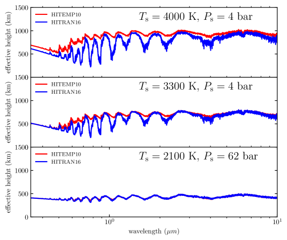
Figure 17: Comparison of effective height of the atmosphere for pure water using two different databases.

References

- Abe & Matsui (1985) Abe, Y. & Matsui, T. 1985. J. Geophys. Res. 90, C545
- Abe & Matsui (1988) Abe, Y. & Matsui, T. 1988, J. of the Atm. Sciences, 45, 21
- B. J. McBride et al. (2002) McBride, B.J., M. J. Zehe, Dr. & Gordon, S. 2002, NASA Glenn Coefficients for Calculating Thermodynamic Properties of Individual Species NASA TP-2002-211556
- Bonati et al. (2019) Bonati, I., Lichtenberg, T., Bower, D.J., Timpe, M.L., Quanz, S.P. 2019, A&A, 621, A125
- Canup (2004) Canup, R. M. 2004, Icarus, 168, 2
- Caroll et al. (1994) Caroll, M.R. & Holloway, J.R., editors, 1994, Volatiles in magmas: Mineralogical society of America, vol. 30, 517 p.
- Clough et al. (1989) Clough, S., Kneizys, F., & Davies, R. 1989, Atmospheric Research, 23, 229
- Ehrenreich et al. (2014) Ehrenreich, D. et al. 2014, A&A, 570, A89
- Elkins-Tanton (2008) Elkins-Tanton, L. 2008, Earth Planet. Sci. Lett. 271(1), 181
- Elkins-Tanton (2011) Elkins-Tanton L. 2011, Astrophys. Space Sci. 332, 359
- Elkins-Tanton (2012) Elkins-Tanton, L. 2012, Annu. Rev. Earth Planet. Sci., 40, 113
- Fiquet et al. (2010) Fiquet, G., Auzende, A.L., Siebert, J., Corgne, A., Bureau, H., Ozawa, H., & Garbarino, G. 2010, Science, 329, 1516
- Fraine et al. (2014) Fraine, J., Deming, D., Benneke, B., Knutson, H., Jordan, A., Espinoza, N., Madhusudhan, N., Wilkins, A. & Todorov, K. 2014, Nature, 513, 526
- Gaillard & Scaillet (2014) Gaillard, F. & Scaillet, B. 2014, Planetary Sci. Lett. 403, 307
- Goldblatt et al. (2013) Goldblatt, C., Robinson, T.D., Zahnle, K. J., & Crisp, D. 2013, Nature Geosci., 6, 661
- Gordon et al. (2017) Gordon, I.E. et al. 2017, J. Quant. Spectrosc. & Radiat. Transfer, 203, 3
- Grenfell et al. (2011) Grenfell, J. L., Gebauer, S., von Paris, P., et al. 2011, Icarus, 211, 81
- Hamano et al. (2013) Hamano, K., Abe, Y., & Genda, H. 2013, Nature, 497(7451), 607
- Hamano et al. (2015) Hamano, K., Kawahara, H., Abe, Y., Onishi, M., & Hashimoto, G. 2015, Astrophys. J. 806(2), 216
- Hedelt et al. (2011) Hedelt, P., Alonso, R., Brown, T., Collados Vera, M., Rauer, H., Schleicher, H., Schmidt, W., ,Schreier, F., and Titz, R. 2011, A&A, 533, A136
- Hedelt et al. (2013) Hedelt, P., von Paris, P., Godolt, M, Gebauer, S., Grenfell, J.L., Rauer, H., Schreier,F., Selsis, F., and Trautmann, T. 2013, A&A, 553, A9
- Herzberg et al. (2000) Herzberg, C., Raterron, P., and Zhang, J. 2000, Geochemistry Geophysics Geosystems, Vol. 1, Issue 11
- Hirschmann (2000) Hirschmann, M. 2000, Geochemistry Geophysics Geosystems, Vol. 1, Issue 10
- Hirshmann (2012) Hirschmann, M. 2012, Earth Planet. Sci. Lett. 341-344, 48
- Hochstaffl et al. (2018) Hochstaffl, P., Schreier, F., Lichtenberg, G., and Gimeno García, S. 2018, Remote Sensing, 10, 2
- Ikoma et al. (2018) Ikoma, M., Elkins-Tanton, L., Hamano, K., Suckale, J. 2018, Space Sci. Rev., 214, 76
- Ingersoll (1969) Ingersoll, A. P. 1969, J. Atmos. Sci. 26, 1191
- Kaltenegger & Traub (2009) Kaltenegger, L., and Traub, W. A. 2009, ApJ, 698, 519
- Kasting (1988) Kasting, J. F. 1988, Icarus, 74, 472
- Kasting (1995) Kasting, J.F. 1995, Planet. Space Sci. 43, 1
- Koparappu et al. (2013) Kopparapu, R. K., Ramirez, R., Kasting, J. F., et al. 2013, Astrophys. Journal, 765
- Lebrun et al. (2013) Lebrun, T., Massol, H., Chassefiere, E., Davaille, A., Marcq, E., Sarda, P., Leblanc, F., & Brandeis, G. 2013, J. Geophys. Res., Planets, 118(6), 1155
- Lide (2000) Lide, D. P., ed. 2000, CRC Handbook of Chemistry and Physics
- Lupu et al. (2014) Lupu, R. E., Zahnle, K., Marley, M., et al. 2014, ApJ, 784, 27
- Marcq (2012) Marcq, E. 2012, J. Geophys. Res. Planets, 117, 1001
- Marcq et al. (2017) Marcq, E., Salvador, A., Massol, H., & Davaille, A. 2017, J. Geophys. Res. Planets, 122, 1539
- Matsui & Abe (1986) Matsui, T., & Abe, Y. 1986a, Nature, 319, 30
- McKay et al. (1991) McKay C.P., Pollack, J.B., & Courtin. R. 1991, Science, 253, 1118
- Meadows et al. (1996) Meadows, V.S. and Crisp, D. 1996, J. Geophys. Res., 101, E2
- Miguel et al. (2011) Miguel, Y., Kaltenegger, L., Fegley, B. & Schaefer, L. 2011, J. Geophys. Res., 101, E2
- Morley et al. (2017) Morley C.V., Kreidberg, L., Rustamkulov, Z., Robinson, T. and Fortney J.J. 2017, Astrophys. J, 850, 2
- Nakajima et al. (1992) Nakajima, S., Hayashi, Y. Y., Abe, Y. 1992, J. Atm. Sciences, 49, 2256
- Nikolaou et al. (2019) Nikolaou, A., Katyal, N., Tosi, N., Godolt, M.,Grenfell, J.L, and Rauer, H. 2019 (to appear in ApJ)
- Pierrehumbert & Gaidos (2011) Pierrehumbert, R. & Gaidos, E. 2011, ApJ, 734, L13
- Ramirez et al. (2014) Ramirez, R.M., Kopparapu, R., Zugger, M.E., Robinson, T.D., Richard F., & Kasting, J.F. 2014, Nature GeoSci. 7, 59
- Rauer et al. (2011) Rauer, H., Gebauer, S., von Paris, P., et al. 2011, A&A, 529, A8
- Rauer et al. (2014) Rauer, H., Catala, C., Aerts, C., et al. 2014, Experimental Astronomy, 38, 249
- Righter & Drake (1999) Righter & Drake, 1999, EPSL, 171, 383
- Rothman et al. (2010) Rothman, L., Gordon, I., Barber, R., Dothe, H., Gamache, R., Goldman, A., Perevalov, V., Tashkun, S., and Tennyson, J. 2010, J. Quant. Spectrosc. & Radiat. Transfer, 111, 2139
- Rothman et al. (2013) Rothman, L., et al. 2013, J. Quant. Spectrosc. & Radiat. Transfer, 130, 4
- Russell et al. (2017) Russell S.S., Ballentine C.J., Grady M.M. The origin, history and role of water in the evolution of the inner Solar System. Philos Trans A Math Phys Eng Sci. 2017;375(2094):20170108
- Salvador et al. (2017) Salvador, V., Massol, H., Davaille, A., Marcq, E., Sarda, P., and Chassefiere, E. 2017, J. Geophys. Res. Planets, 122, doi:10.1002/2017/JE005286
- Segura et al. (2003) Segura, A., Krelove, K., Kasting, J. F., et al. 2003, Astrobiology, 3, 689
- Schaefer et al. (2004) Schaefer, L. & Fegley, B., Jr. 2004, Icarus, 168, 215
- Schaefer & Fegley (2010) Schaefer, L. & Fegley, B., Jr. 2010, Icarus, 208, 438
- Schaefer & Fegley (2007) Schaefer, L., & Fegley, B. 2007, Icarus, 186, 462
- Schaefer et al. (2016) Schaefer, L., Wordsworth, R. D., Berta-Thompson, Z., & Sasselov, D. 2016, ApJ, 829, 63
- Schaefer et al. (2017) Schaefer, L. & Fegley, B., Jr. 2017, Astrophys. J, 843, 120
- Schreier et al. (2014) Schreier, F., Gimeno García, S., Hedelt, P., Hess, M., Mendrok, J., Vasquez, M., & Xu, J. 2014, J. Quant. Spectrosc. & Radiat. Transfer, 137, 29
- Schreier et al. (2018a) Schreier, F., Städt, S., Hedelt, P. and Godolt, M. 2018a, Mol. Astrophys. 11, 1
- Schreier et al. (2018b) Schreier, F., Milz, M., Buehler, S.A., and Clarmann, T. von. 2018b, J. Quant. Spectrosc. & Radiat. Transfer, 211, 64
- Snyder (2016) Snyder, C.A., Glen research center, Feb 2016, URL https://www.grc.nasa.gov/WWW/CEAWeb/
- Solomatov (2007) Solomatov, V. 2007, Treatise on Geophysics, 9, 91
- Tosi et al. (2017) Tosi, N., Godolt, M., Stracke, B., Ruedas, T., Grenfell, J. L., H’́oning, D., Nikolaou, A., Plesa, A.-C., Breuer, D., and Spohn, T. 2017, A&A, 605, A71
- Vasquez et al. (2013a) Vasquez, M., Schreier, F., Gimeno García, S., Kitzmann, D., Patzer, B., Rauer, H. and Trautmann, T. 2013a, A&A, 549, A26
- Vasquez et al. (2013b) Vasquez, M., Schreier, F., Gimeno García, S., Kitzmann, D., Patzer, B., Rauer, H. and Trautmann, T. 2013b, A&A, 557, A46
- Vasquez et al. (2013c) Vasquez, M., Gottwald, M., Gimeno García, S., Krieg, E., Lichtenberg, G., Slijkhuis, S., Schreier, F., R. Snel, R., and Trautmann., T. 2013c, ASR, 51, 835
- Wakeford et al. (2017) Wakeford, H.R., et al. 2017, Science, 356, 628
- Wagner & Pruß (2002) Wagner, W., & Pruß, A. 2002, J. Phys. Chem. Ref. Data, 31, 2
- Wit et al. (2016) Wit et al., Nature, 537, 69
- Wordsworth (2012) Wordsworth, R. 2012, Icarus, 219, 267
- Wordsworth & Pierrehumbert (2013) Wordsworth, R.D. and Pierrehumbert, R.T. 2013, ApJ, 778, 154
- Wordsworth & Pierrehumbert (2013) Wordsworth, R.D. & Pierrehumbert, R., 2013, Science, 339, Issue 6115, pp 64-67
- Wu et al. (2018) Wu et al., JGR Planets, 2018, doi:10.1029/2018JE005698
- Wunderlich et al. (2018) Wunderlich, F., Godolt, M., Grenfell, J.L., Städt, S., Smith, A.M.S., Gebauer, S., Schreier, F., Hedelt, P., Rauer, H. 2018, accepted in A&A
- Xu et al. (2018) Xu, J., Schreier, F., Wetzel, G., de Lange, A., Birk, M., Trautmann, T., Doicu, A. and Wagner, G. 2018, Remote Sensing, 10, 2
- Yang et al. (2016) Yang, J., Leconte, J., Wolf, E.T., Goldblatt, C., Feldl, N., Merlis, T., Wang, Y., Koll, D., Ding, F., Forget, F., and Abbot, D.S. 2016, Astrophys. J, 826, 222
- Zahnle (2005) Zahnle. K, Schaefer. L, and Fegley B. 2010, Cold Spring Harb Perspect Biol. 2, 10.
- Zahnle et al. (2010) Zahnle,, K., Schaefer, L., & Fegley, B. 2010, Cold Spring Harb Perspect Biol., v.2(10)
- Zhang & Herzberg (1994) Zhang, J., and Herzberg, C. 1994, J. Geophys. Res., 99(B9), 17, 729–17, 742