Generating superpixels using deep image representations

Abstract

Superpixel algorithms are a common pre-processing step for computer vision algorithms such as segmentation, object tracking and localization. Many superpixel methods only rely on colors features for segmentation, limiting performance in low-contrast regions and applicability to infrared or medical images where object boundaries have wide appearance variability. We study the inclusion of deep image features in the SLIC superpixel algorithm to exploit higher-level image representations. In addition, we devise a trainable superpixel algorithm, yielding an intermediate domain-specific image representation that can be applied to different tasks. A clustering-based superpixel algorithm is transformed into a pixel-wise classification task and superpixel training data is derived from semantic segmentation datasets. Our results demonstrate that this approach is able to improve superpixel quality consistently.

I Introduction

Many deep learning based applications in computer vision operate on a grid of pixels and use convolutions trained end-to-end. However, popular algorithms have successfully leveraged image segmentation to group pixels into superpixels, reducing the input dimensionality while preserving the semantic content needed to address the task at hand [1]. Superpixels are efficient image priors that tend to transfer across tasks and reduce the data needed to train models, which can be very beneficial for domain adaptation and weakly supervised settings, e.g. weakly supervised image segmentation [2]. Graph-based convolutional networks [3] also allow applications of deep learning beyond grid-like inputs. Some works [4] explored the inclusion of superpixels in deep learning pipelines.

The hand-crafted design of superpixels algorithms limits our ability to tune image segmentations to a specific image domains, such as infrared, medical, of spatio-temporal data. Given the focus on efficiency, superpixels have often been designed to operate on color features only; image segmentations could however incorporate higher-level image representations. We consider extensions to a standard superpixel algorithms incorporating higher-level unsupervised or supervised image features. We also study paths to fine-tune a superpixel segmentation algorithm to a specific modality. There has been few research on trainable superpixels. In parallel to our work, Wei-Chih Tu et al. [5] have developed a trainable variant of graph-based superpixel algorithms using trainable superpixel affinities. Our approach is based on a clustering algorithm, which tends to be faster and more suited for real-time applications due to their iterative nature [6].

II SLIC algorithm

Several comparisons indicate that the Simple Linear Iterative Clustering (SLIC) [7] image segmentation algorithm offers both good speed and performance [6][8]. It uses a clustering approach similar to $k$-means, and usually operates on images in the CIELAB color space. After initialization of the cluster centers along a grid, a two-step iterative process refines clusters until convergence. First, the pixels are assigned to the closest cluster center in a joint $5$-dimensional space of colors ($L$, $a$ and $b$) and spatial ($x$ and $y$) components. The weighted $L2$ distance includes a compactness parameter $\sigma$ to balance between colors and space. Second, the cluster centers are updated based on the pixel assignments. Finally, after convergence, a simple connected components algorithm enforces connectedness of the image segments.

III Augmenting SLIC with deep representations

III-A Deep representations

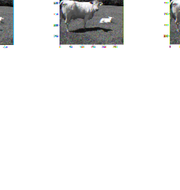
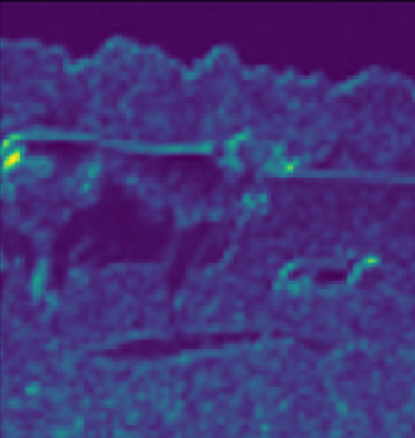
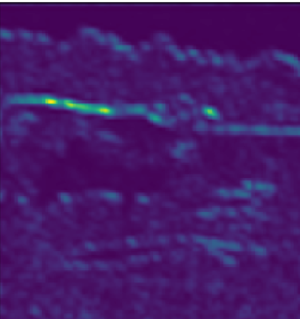
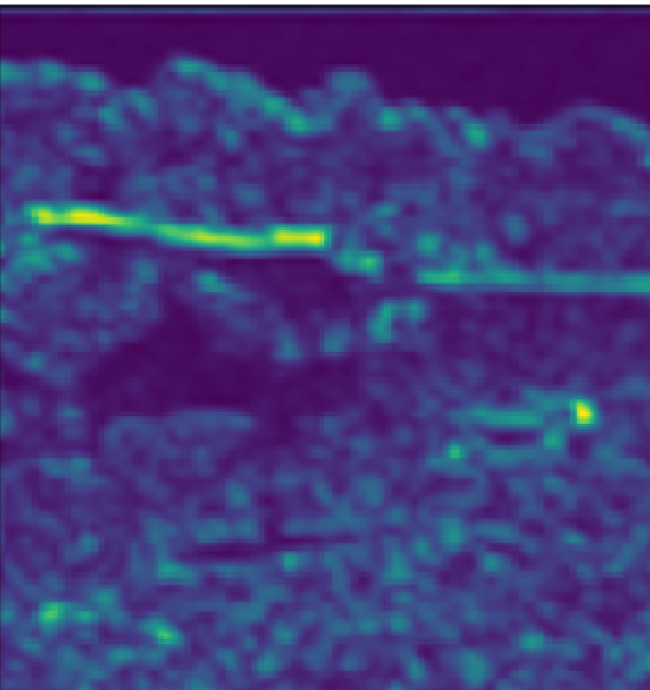
We experiment with SLIC beyond the original $Lab$ features. Deep representations capturing textures, gradients and edges in the image can be extracted from convolutional neural networks. Their structure is similar to multi-channel images, often having a lower resolution than the original image. Each channel represents an image feature. These features can be unsupervised, as in the case of scattering features [9] (Fig. 1), or trained for a particular vision task. Segmentation networks such as ENet [10] have convolutional layers behaving like feature extractors. As we aim to integrate superpixels in a deep architecture, the features can be provided at no extra computational cost. Unsupervised scattering networks are similar to convolutional neural networks whose filters are fixed as wavelets. We use scattering networks with a receptive field of $4\times 4$ for our experiments on $256\times 256$ images, generating $M=81$ features maps of size $64\times 64$ per image channel.

Figure 1: Input image and some scattering features

III-B Inclusion in SLIC

For a particular pixel, we have image features $f_{1},f_{2},\ldots f_{M}$. To incorporate the image features into SLIC, we augment the number of image channels. The scattering features are upscaled and concatenated with the input image (Fig. 2). The final image of size $W\times H\times(M+3)$ can be used in the SLIC algorithm, where the $Labxy$ clustering space now becomes a larger $L,a,b,f_{1},\ldots,f_{M},x,y$ space. The SLIC color distance is extended and individual feature maps are weighted with coefficients $\beta_{1}...\beta_{M}$. The distance in the color space between pixel $i$ and cluster $k$ is then defined as

$$d_{c}^{2}= \alpha_{1}(L_{k}-L_{i})^{2}+\alpha_{2}(a_{k}-a_{i})^{2}+\alpha_{3}(b_{k}-b_{i})^{2}$$ (1)

$$+\sum_{m=1}^{M}\beta_{m}(f_{m,k}-f_{m,i})^{2}\ .$$

Figure 2: The feature maps are upscaled and concatenated with the original image. A SLIC algorithm with extended color distance measure is applied on the multi-channel image.

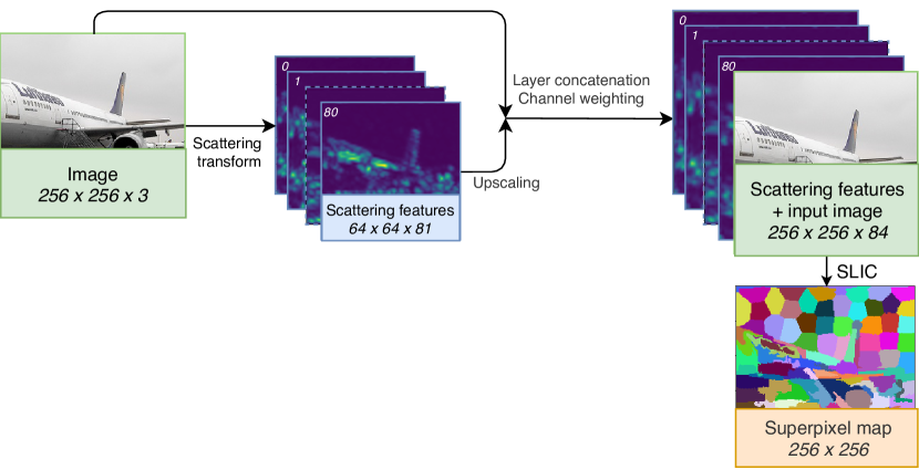
Our first experiments investigate the impact of scattering features by manually tuning the inclusion of scattering features on the lightness component $L$ only. We define binary weights $\beta_{m}$ based on the visual appearance of the features. Layers originating from strong edge detectors are left out since they are of no use in clustering. We also varied the relative importance of the extra features compared to the color components and selected the best-scoring approach (out of 10 different ones) for evaluation (Section VII-B).

IV Trainable superpixel algorithm

Manual selection and weighting of features in the distance measure is a tedious process, requiring visual examination of features and an exhaustive search for optimal weights. In addition, the distance measure (1) might not have enough flexibility to integrate those features properly. We research a trainable superpixel algorithm incorporating a neural network that can tune superpixels to a certain image set.

IV-A Clustering as a classification problem

The SLIC superpixel algorithm uses a top-down approach: the algorithm iterates over all cluster centers and calculates a distance measure to all pixels in the $2S\times 2S$ neighborhood around the cluster center. An equivalent bottom-up approach would be to iterate over all pixels and calculate a distance measure between the pixel and all the clusters in the $2S\times 2S$ region around the pixel. The pixel is then assigned to the cluster being the closest in the $5D$ clustering space of SLIC with $Labxy$ components.

This is in fact a classification problem: assign each pixel to one of the clusters in the spatial neighborhood. While SLIC solves this classification problem using a distance measure, we rather avoid to train a regression because distances improving superpixel performance are hard to define. We propose to use a neural classifier for the assignment task: it considers a fixed amount of spatially closest clusters in the neighborhood and assigns the pixel to one those depending on their features.

IV-B Bottom-up trainable superpixel algorithm

The algorithm (Algorithm 1) works in a similar way to SLIC. Clusters are first initialized on a grid. Then, clusters are formed using a two-step iterative procedure: the first step assigns each pixel to one of the $Q$ spatially closest clusters, using classification based on the features of these clusters and the pixel of interest. $Q$ is a parameter: higher means more flexibility at the cost of more computations. Afterwards, the features and position of the newly formed clusters are calculated by averaging the features and positions of the pixels assigned to those clusters. This iterative procedure is done for a fixed amount of iterations. Finally, a connected components algorithm is used to transform clusters into proper superpixels.

A sequential implementation as described here would be slow: the large amount of individual network evaluations limits the performance. We implemented a version that generates large batches and evaluates these on a GPU. The algorithm can also easily be parallelized because every pixel is processed independently.

# Initialization

Initialize cluster centers $C_{k}=[l_{k},a_{k},b_{k},x_{k},u_{k}]^{T}$ by sampling pixels at regular grid steps $S$.

label $l(i)\leftarrow-1$ for each pixel $i$

repeat

    # Clustering iteration

    for all pixels $p_{i}$ do

         closest_idx $\in\mathbb{R}^{1\times Q}\leftarrow$ Q cluster centers nearest to $p_{i}$

         input $\leftarrow$ features of pixel $p_{i}$ and Q nearest clusters

         output $\in\mathbb{R}^{1\times Q}\ \leftarrow$ network(input)

         best_cluster_id $\leftarrow$ closest_idx[argmax(output)]

         $l(i)\leftarrow$ best_cluster_id

    end for

    Compute new cluster centers and features based on $l$

until number of iterations reached

Algorithm 1 Bottom-up trainable superpixel algorithm

IV-C Neural network architecture

The input vector for the classification of a single pixel consists of several parts:

• $M$ pixel features, for example the pixel color and other features extracted using deep representations.

• $Q$ spatial distances to the $Q$ closest clusters. In order to have a single neural network for multiple superpixel sizes and compactness parameters, the distance is normalized: $D_{q}={\sigma*distance_{q}}/{step\_size}$, with $distance_{q}$ the pixel distance between pixel and cluster center $k$.

• $Q\times M$ feature differences between the input pixels and cluster centers.

The network outputs a vector of size $Q$, where each element $q=1...Q$ denotes the probability of the pixel belonging to cluster with index $q$. We aim for a small network and look at the problem as a typical classification problem. A fully connected network would not exploit the similarity between different parts of the input vector. An efficient architecture is made up of three parts: normalization, dimensionality reduction and classification (Fig. 3). The Dimensionality Reducer for Pixels (DRP) modules transforms the pixel features to a smaller space, while the Dimensionality Reducer for Clusters (DRC) is applied on the pixel-cluster differences. Weights are shared between similarly-named modules to reduce the number of trainable parameters. The final fully connected network (FC) does the actual classification.

Figure 3: Classifier with dimensionality reduction modules. The weights of the Dimensionality Reducer for Clusters (DRC) modules are shared to reduce the amount of trainable weights.

Figure 4: Diagram of the training and evaluation procedure. Training data for the classifier is derived from a semantic segmentation dataset. The input vectors and labels are used to train the classifier. Afterwards, the trained classifier is integrated in the trainable superpixel algorithm and results are evaluated on the test dataset.

V Generating training labels

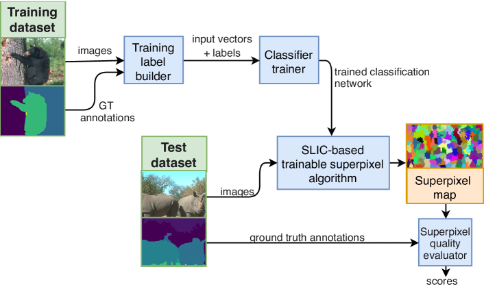
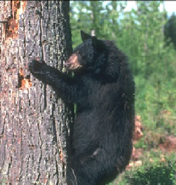
The classifier requires training labels, indicating which cluster the pixel should be assigned to according to ground truth. Since no database with superpixel annotations exist, we derive a label set from semantic segmentation databases such as Cityscapes [11] and BSDS [12] (Fig. 4).

V-A SLIC-based labels

We use the SLIC distance measure as a starting point to produce labels. SLIC replication requires to calculate the SLIC distance measure to the $Q$ closest clusters of the classifier and pick the closest cluster according to this measure. The pixel label is then set to this cluster. Replicating SLIC would not force the classifier to include the features extracted from deep representations in its decision process. To improve superpixels beyond SLIC, we use ground truth annotations for semantic segmentation to correct wrong labels, where the pixel would be assigned to a cluster in a different ground truth segment. SLIC makes these mistakes when regions have approximately the same colors, but the classifier can use deep representations to discriminate between the two regions. When generating a label for a cluster, we only consider assignment to clusters lying mainly in the same ground truth segment as the pixel being classified.

Ground truth segmentations are typically much larger than superpixels and the amount of pixels being corrected by the ground truth segmentation is small. The classifier thus primarily replicates SLIC and ignores the corrected labels. A multi-label loss could take into account that multiple clusters are good candidates, but we couldn’t achieve satisfactory results using this approach. We solve the problem by using principles of hard-example mining: the set of labels is carefully chosen to improve the training process.

Hard-example mining on SLIC mistakes

We try to train the classifier by only retaining labels that were corrected by the ground truth annotations. Our experiments indicate that this is too strict and degrades superpixel performance.

Hard-example mining at segmentation edges

A less strict method would be to only consider pixels near ground truth edges. Labels in the middle of the ground truth segments have a lot of ambiguity: we cannot be sure whether the assigned cluster is really in the same part of the object. Labels at the edges have more discriminative power. We call these unambiguous labels. Our implementation does not exactly select pixels near the edge; it is easier to count the amount of different ground truth segments of the $Q$ closest clusters. Thus, we restrict the training set to pixels that have candidate clusters in at least a chosen amount of different ground truth segments.

V-B Weakly supervised labeling

Using the SLIC distance measure to generate pixel labels offers a good starting point but might also restrict the adaptability of the classification network. One could label a pixel to a random cluster in the same segment. This obviously generates very noisy superpixels. Picking the closest cluster in the same segment has the opposite problem: the spatial component is emphasized too much. Again, we leverage the principles of hard-example mining to build a better training set. We limit the training set to pixels having candidate clusters in at least $X$ segments, with an optimal $X$ to be determined experimentally (Fig. 5). Interestingly, our experiments indicate that a higher value for $X$ produces more compact clusters (Fig. 6). The reduced amount of ambiguity increases the importance of the spatial component: the network learns that two pixels next to each other might have very different features, while having very similar spatial distances to the spatially closest clusters.

(a) At least 2 different distances

(b) At least 4 different distances

(c) At least 6 different distances

Figure 5: Hard-example mining: only labels produced by clusters in minimum $X$ different ground truth segments are used for training.

(a) At least 2 different distances

(b) At least 4 different distances

(c) At least 6 different distances

Figure 6: Superpixel output for hard-example mining. Restricting the the label set by removing ambiguous labels produces more compact superpixels.

(a) Input image

(b) Single GT edge map

(c) Combined edge map

Figure 7: BSDS500: multiple ground truth annotations are combined in a single edge map. Stronger borders in the image have stronger appearance in the edge map.

V-C BSDS ground truth edges

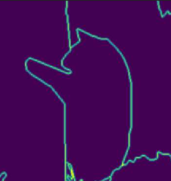
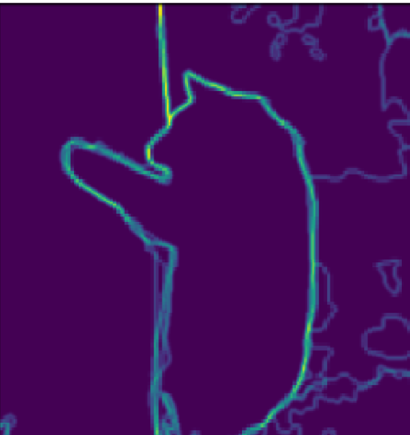
More refined semantic segmentations provide more accurate labels. We considered several semantic segmentation datasets: PASCAL VOC [13], Cityscapes [11] and BSDS500 [12]. Cityscapes and BSDS both have high-quality ground truth annotations, but BSDS has multiple of them for a single image. Typically, object borders in natural images are not clearly delineated and multiple independent ground truth segmentations help to handle these cases. We combine the 5 individual ground truth annotations in a single ground truth edge map (Fig. 7). This also defines a new distance measure: more edges between a pixel and cluster indicate a greater distance and less likelihood to be assigned to that cluster.

VI Training a distance measure

The proposed network interprets the classification task as a typical deep learning problem. We were not able to replicate the SLIC distance measure exactly, although superpixel output was similar. We note that the SLIC distance measure could be perfectly replicated by squaring each element of the input vector and removing the batchnorm layer: the elements of the input vector then become the individual terms of the SLIC distance measure. By making the different parts of the network independent, the trained modules can be seen as distance functions (Fig. 8). The network then learns a regression by training a classification. We verified that the network can almost perfectly replicate the SLIC distance measure (Table II). When using a single linear layer, the network in fact learns the weights of Equation 1. These weights can then be integrated in the top-down approach of SLIC, resulting in a very efficient trainable superpixel algorithm running on CPU.

Figure 8: Classifier with distance function modules. The amount of clusters considered during classification can be changed easily. The network learns a distance function between clusters and pixels using classification labels.

Table I: Performance comparison of superpixel methods in this work

500 BSDS color images, superpixel size 16, compactness 10 Method IoU Rec MDE UE CO SLIC (reference) 0.907 0.809 0.911 0.101 0.324 Manual tuning: inclusion of features using an extended distance measure 0.913 0.819 0.870 0.095 0.328 Deep learning classification network: SLIC with GT-corrected and hard-example labels ($X=3$) 0.910 0.800 0.942 0.097 0.328 Deep learning classification network: Weakly supervised hard-example labels ($X=6$) 0.913 0.796 0.954 0.094 0.307 1-layer regression network 0.912 0.819 0.874 0.095 0.325 3-layer regression network 0.912 0.824 0.855 0.094 0.320

VII Evaluation and results

VII-A Metrics

Superpixel performance is evaluated on 500 BSDS500 [12] color images. Superpixels are evaluated with size $16$, compactness $10$ (determined optimal for the standard SLIC) and 5 clustering iterations. We use several metrics common in superpixel evaluation: Boundary recall (Rec) represents the adherence to ground truth boundaries (higher is better). Mean distance to edge (MDE) [14] measures the average distance between the ground truth border and closest superpixel edge (lower is better). Superpixel leakage into different ground truth segments is quantified by the undersegmentation error (UE) (lower is better). Multiple variants exist, we use the definition of Neubert and Protzel [8]. The regularity and compactness of superpixels is measured by the compactness (CO) metric [15]. More regular superpixels are generally preferred. For a fair comparison, the compactness parameters of different methods are chosen so their resulting output compactness is similar. We define an additional intersection-over-union (IoU) metric similar to the one often used in segmentation benchmarks. This metric measures the maximum achievable performance when using superpixels in a segmentation pipeline.

VII-B Extended distance measure with manual tuning

As a first experiment, we evaluate the inclusion of scattering features in the extended distance measure for SLIC (Section III). The scattering transformation is applied on the lightness channel $L$ of the image (converted to the $CIELAB$ color space) and we manually select the most important representations. We refer to this method as ‘Manual tuning’ and Table I shows that all metrics are improved. Mainly the mean distance to edge and undersegmentation metrics are impacted: the low-resolution features do not help at a pixel-scale level, but avoid superpixel leakage. The difference is larger at lower compactness values (Fig. 10). Evaluating the methods for their own optimal compactness, improvement of MDE is 9.4% compared the 4.3% improvement for $\sigma=10$. The approach with scattering features benefits from the increased flexibility, while SLIC performance decreases. Superpixels incorporating deep representations also consistently perform better (Fig. 9): most images are slightly improved. In addition, we experimented with greyscale images and the effect of scattering features is even stronger.

Figure 9: Consistency of results: scores per image for the mean distance to edge (lower is better) and undersegmentation error (lower is better) metric. The SLIC implementation with scattering features and manually tuned weights scores consistently better.

Figure 10: Influence of compactness parameter $\sigma$ on MDE and UE metrics for the manually tuned method.

VII-C Trainable superpixels

Trainable superpixels should be able to improve superpixel quality without having to manually tune the distance measure weights. Quality assessment of the trainable superpixels is a three-stage process: a label set is generated, a classifier is trained on these labels and the superpixel algorithm using the trained classifier is evaluated. We selected the most promising label methods for evaluation on $256\times 256$ BSDS500 images and tested scattering and ENet features. The 243 scattering features have a receptive field of $4\times 4$ and spatial dimensions of $64\times 64$. The ENet features are extracted from the first convolutional layer, designed to be feature extractor and consisting of filters having a receptive field of $3\times 3$. They have a better spatial resolution of size $128\times 128$, but there are only 16 features.

We selected a simple network with an architecture as in Fig. 3, where the dimensionality reducers DRP/DRC are 2-layer networks (hidden layers of 100 and 15 neurons) and the classification network FC is a 4-layer network (hidden layers of size 120, 105 and 15, output layer of 7 neurons). All activation functions are rectified linear units (ReLU). We call this network the ‘Deep learning classification network’. We also test regression architectures as in Fig. 8 with a single linear layer for the distance measure module: this is in fact just a weighted addition of the squared pixel-cluster differences. This approach is called ‘1-layer network’. In addition, we evaluate a network where the single layer is expanded to 3 layers (‘3-layer’).

We trained on several label methods and experimented with different variations of hard-example mining for both SLIC-based labels and weakly supervised labels. Our experiments found that more engineered methods performed better. The best SLIC-based method corrects labeling mistakes with the segmentation ground truth and applies hard-example mining, with parameter $X=3$, in order to remove ambiguous labels. The best weakly supervised label method also removes ambiguous labels, but with parameter $X=6$, retaining clusters lying in at least 6 different ground truth segments.

VII-D Validation loss

Table II: Validation loss for different training methods, features and networks

Label method Scat F ENet F Deep learning classification-based network SLIC replication 0.184 0.210 SLIC with GT-corrected hard-example labels ($X=3$) 0.786 0.746 Weakly supervised hard-example labels ($X=6$) 1.413 1.400 1-layer regression-based network SLIC replication 0.016 0.035 SLIC with GT-corrected hard-example labels ($X=3$) 0.970 2.885 3-layer regression-based network SLIC with GT-corrected hard-example labels ($X=3$) 0.731 0.960

As different labeling methods employ different loss functions, we cannot directly compare the values of these loss functions on the validation set. For a single label method, a comparison between network architectures and features is possible and serves as an indication for resulting superpixel quality. Table II shows that scattering features and ENet features achieve similar validation losses in most cases. Unsurprisingly, the 3-layer regression network performs better than the 1-layer one, and it also performs slightly better than the classification-based network that used batch normalization and dimensionality reduction modules.

VII-E Superpixel quality

The superpixel quality for each of these methods is compared in Table I. The 3-layer regression-based network, having the lowest validation loss, also achieves the best metric scores. Superpixel quality is improved over standard SLIC and also over the manually tuned method of Section III. Comparing methods visually (Fig. 12) shows that the manually tuned method tends to concentrate superpixels around object borders. This effect is not seen in the trained superpixels. During evaluation of manually tuned superpixels, we already discovered that the extra features mainly influence the mean distance to edge and undersegmentation metrics and the same effect can be seen here. The weakly supervised method has surprisingly similar scores to SLIC and during our tests we noticed that the variation in compactness was much lower (Fig 11).

Figure 11: Scatter plot of the scores per image for undersegmentation (lower is better) and compactness metrics. The trainable approach using weakly supervised labels improves the undersegmentation error quite consistently and the produced superpixels have a low variation in compactness compared to SLIC.

VIII Conclusion

Superpixels are image priors that tend to transfer across tasks. This works elaborates on a trainable approach for superpixels incorporating deep image representations. We introduce several new ideas not yet addressed in research: we include deep representations in a superpixel algorithm, build a set of superpixel training labels from segmentation annotations and devise a trainable superpixel algorithm. We demonstrate that a simple inclusion of deep representations by extending the SLIC distance measure improves superpixel quality in a consistent way. The trainable approach can surpass the scores of the simple inclusion, but requires appropriate training labels. The performance increase could be limited by the dataset and features used in our experiments. We used natural images, which have a high variability in features. We believe larger performance increases can be achieved by targeting specific modality, such as medical imaging. More specialized features can be incorporated, possibly having a less restricted receptive field than the scattering features. We hope that our analysis paves the way to the inclusion of trainable superpixels in deep learning pipelines.

(a) SLIC

(b) Manual tuning

(c) Trainable (3-layer)

Figure 12: Outputs of different superpixel methods. The manual tuning method tends to concentrate superpixels around object edges, for example at the bear’s paw.

References

- [1] Brian Fulkerson, Andrea Vedaldi and Stefano Soatto “Class segmentation and object localization with superpixel neighborhoods” In 12th Int. Conf. on Computer Vision, 2009, pp. 670–677 IEEE
- [2] Suha Kwak, Seunghoon Hong and Bohyung Han “Weakly Supervised Semantic Segmentation Using Superpixel Pooling Network” In AAAI, 2017, pp. 4111–4117
- [3] Thomas N Kipf and Max Welling “Semi-Supervised Classification with Graph Convolutional Networks” In arXiv:1609.02907, 2016
- [4] Mathijs Schuurmans, Maxim Berman and Matthew B Blaschko “Efficient semantic image segmentation with superpixel pooling” In arXiv preprint arXiv:1806.02705, 2018
- [5] Wei-Chih Tu1 Ming-Yu Liu, Varun Jampani2 Deqing Sun Shao-Yi, Chien1 Ming-Hsuan Yang and Jan Kautz “Learning Superpixels with Segmentation-Aware Affinity Loss”
- [6] David Stutz, Alexander Hermans and Bastian Leibe “Superpixels: an evaluation of the state-of-the-art” In Computer Vision and Image Understanding 166 Elsevier, 2018, pp. 1–27
- [7] Radhakrishna Achanta et al. “SLIC Superpixels Compared to State-of-the-Art Superpixel Methods” In IEEE Trans. on Pattern Analysis and Machine Intelligence 34.11 IEEE, 2012, pp. 2274–2282
- [8] Peer Neubert and Peter Protzel “Superpixel benchmark and comparison” In Proc. Forum Bildverarbeitung, 2012, pp. 1–12
- [9] Edouard Oyallon, Eugene Belilovsky and Sergey Zagoruyko “Scaling the Scattering Transform: Deep Hybrid Networks” In Proc of the IEEE Conf. on Computer Vision and Pattern Recognition (CVPR), 2017, pp. 5618–5627
- [10] Adam Paszke, Abhishek Chaurasia, Sangpil Kim and Eugenio Culurciello “ENet: A Deep Neural Network Architecture for Real-Time Semantic Segmentation” In arXiv preprint arXiv:1606.02147, 2016
- [11] Marius Cordts et al. “The Cityscapes Dataset for Semantic Urban Scene Understanding” In Proc. of the IEEE Conf. on Computer Vision and Pattern Recognition (CVPR), 2016
- [12] Pablo Arbelaez, Michael Maire, Charless Fowlkes and Jitendra Malik “Contour Detection and Hierarchical Image Segmentation” In IEEE Trans. Pattern Anal. Mach. Intell. 33.5 Washington, DC, USA: IEEE Computer Society, 2011, pp. 898–916 DOI: 10.1109/TPAMI.2010.161
- [13] M. Everingham, L. Van Gool, C… Williams, J. Winn and A. Zisserman “The PASCAL Visual Object Classes Challenge 2012 (VOC2012) Results”, http://www.pascal-network.org/challenges/VOC/voc2012/workshop/index.html
- [14] Wanda Benesova and Michal Kottman “Fast superpixel segmentation using morphological processing” In Proc. of the Int. Conf. on Machine Vision and Machine Learning (MVML), 2014
- [15] Alexander Schick, Mika Fischer and Rainer Stiefelhagen “Measuring and evaluating the compactness of superpixels” In 21st International Conference on Pattern Recognition (ICPR), 2012, pp. 930–934 IEEE