Emergence of Brain Rhythms: Model Interpretation of EEG Data

Abstract

Electroencephalography (EEG) monitors —by either intrusive or noninvasive electrodes— time and frequency variations and spectral content of voltage fluctuations or waves, known as brain rhythms, which in some way uncover activity during both rest periods and specific events in which the subject is under stimulus. This is a useful tool to explore brain behavior, as it complements imaging techniques that have a poorer temporal resolution. We here approach the understanding of EEG data from first principles by studying a networked model of excitatory and inhibitory neurons which generates a variety of comparable waves. In fact, we thus reproduce $\alpha$, $\beta,$ $\gamma$ and other rhythms as observed by EEG, and identify the details of the respectively involved complex phenomena, including a precise relationship between an input and the collective response to it. It ensues the potentiality of our model to better understand actual mind mechanisms and its possible disorders, and we also describe kind of stochastic resonance phenomena which locate main qualitative changes of mental behavior in (e.g.) humans. We also discuss the plausible use of these findings to design deep learning algorithms to detect the occurence of phase transitions in the brain and to analyse its consequences.

Introduction

There has been a growing interest in investigating the occurrence of phenomena associated with thermodynamic-like phase transitions and criticality during the functioning of neural media by means of novel experimental techniques, analysis of available connectome data, and biological-inspired theoretical approaches; see, e.g., [1, 2, 3, 4, 5], and references therein. In particular, a sort of brain critical behavior —mimicking essential features of phase transition phenomena such as condensation and ferromagnetism— is now believed to be at the origin of the observed good processing throughout the brain of signals coming from different areas and the senses [6, 7, 5]. That is, there has recently emerged definite evidence that weak signals are optimally transferred and even enhanced in a noisy environment when the system is in a well-defined region with great susceptibility which happens to separate neuron dynamic “phases”, i.e., areas in parameter space in which the brain shows qualitatively different kinds of behavior [3, 4]. Ref. [3] also presents a feasible procedure to experimentally detect phase transitions and their details during the performance of actual brains. Following this promising path, in the present paper we investigate the possibility of visualizing phase transitions during brain operation by using easily-extracted brain-activity data obtained from EEG (by the same token, magnetoencephalograph) recordings. It ensues what we hope is a convenient tool to monitor in vivo changes between different dynamic behaviors of the cerebral activity. It may also follow how to design specific stimuli to control these dynamic phases and eventually modify some of their properties, e.g., in cases of dysfunction.

More specifically, we here present and discuss an EEG neural-activity model which generalizes and formalizes a previous one [8]. We link this to a familiar mathematical framework, improve the temporal precision of the original setting, include an appropriate tuning of the noise, and consider the possibility of an input signal that makes the model useful to reveal and analyze new intriguing phenomena. The new setting allows us to deep on how oscillation patterns, e.g., as observed by electroencephalography, emerge reflecting different dynamic activity, and we thus infer the precise role of the intrinsic noise in causing familiar rhythms in the human brain. It ensues that not only $\alpha$ rhythms but also $\beta$, $\gamma$ and ultrafast oscillations are all just a form (at different levels) of the same “noise” as it is filtered (in a way that our model clarifies) by the neural network itself. That is, one may conclude that the cause for brain waves is universal within this context, which allows us to consider a unique mechanism for any of the mentioned voltage fluctuations with only a relevant parameter. This, we show, is the intensity of the sum of all the inputs, either noisy or constant, reaching the network from the outside, and we succeed in parametrizing it. Consequently, we are able to rigorously relate the occurrence of phase transitions —actually, having a non-equilibrium nature [9, 4]— in the brain with different possible dynamic behaviors which are revealed by the easily-observed EEG rhythms mentioned. It is with this aim that we here use a network, which involves both excitatory and inhibitory units, where a random input is sufficient to generate different brainwaves, some of them respectively corresponding to $\alpha$, $\beta$, $\gamma$ and ultrafast oscillations. We also precisely relate the intensity of the input and the frequency of the resulting dynamic response and —following a method first reported in [3]—we show how to use an external signal in a simple experiment to identify the undergoing phase changes and other details during brain operation using the mechanism of stochastic resonance (SR) [10].

We believe there are two extra, side results from the present model. One is that it may be useful to design appropriate deep or machine learning neural networks to learn about possible phase transitions in the brain and their features – including critical exponents and universality classes – from raw data in actual EEG recordings [11]. Also our results here can be used to built similar algorithmic tools based instead on the SR phenomenon [12] to optimally learn feature representation in the presence of noise from EEG time series [13].

Model and method

Consider, for simplicity and ease of representation, a regular two-dimensional network on a torus —in which periodic boundary conditions avoid surface effects and simulate a larger system— with $N$ nodes each holding either an excitatory (E) or an inhibitory (I) neuron as depicted in Fig.1. They interact with each other such that any E excites one or more Is as long as the membrane voltage of the former exceeds a given threshold potential, and when any I exceeds its own threshold it will inhibit a group of Es (negative feedback). No delays are considered, which might exclude very extensive networks, and we also neglect both positive feedback of Es (any E stimulating another E) and negative feedback of Is (any I inhibiting other I). Furthermore, according to histological data —showing that, in portions of the cortex, there are about four times more excitatory than inhibitory neurons [14, 15, 16, 17]— the E/I ratio is assumed here to be 4, so that any I neuron receives effective excitatory inputs from 32 surrounding Es and any I neuron projects upon 12 surrounding Es, as illustrated in Fig.1A.

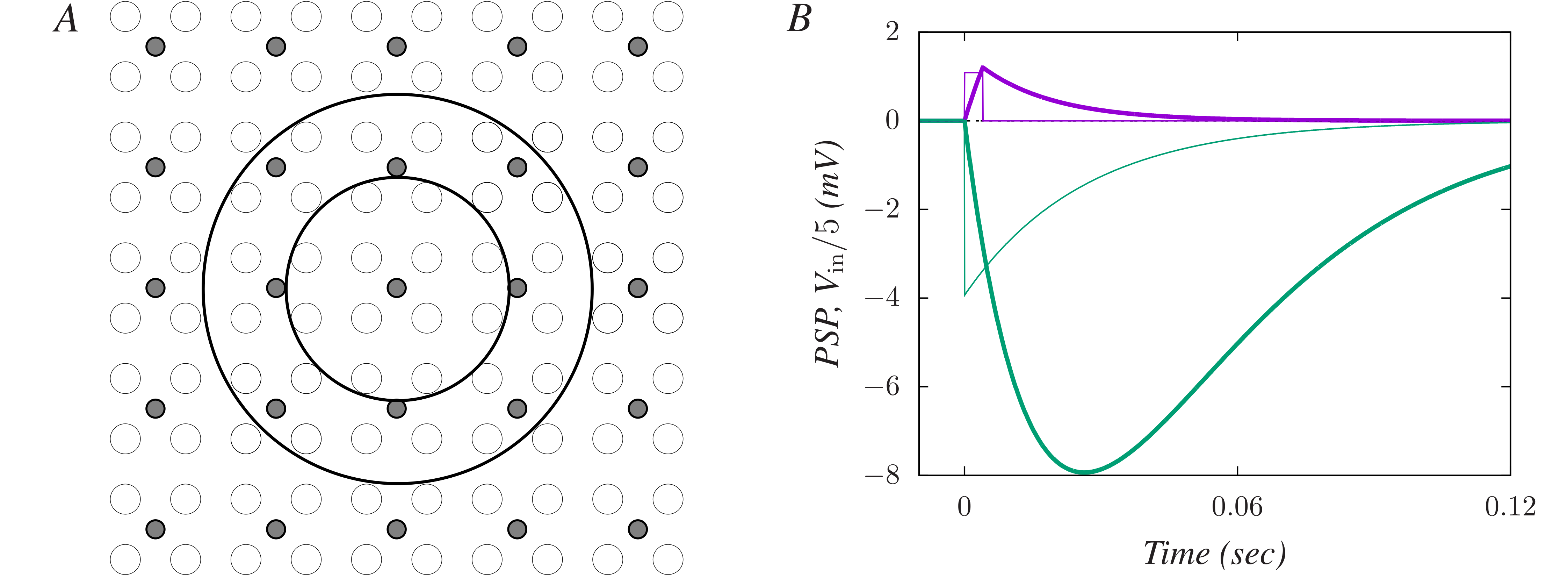
Figure 1: Model features. Left panel: a portion of the actual network topology (we here in practice considered $N=180$ nodes), where filled circles stand for inhibitory (I) neurons and open circles represent excitatory (E) neurons. In order to mimic biological conditions (and following [8]), the largest of the two concentric circles drawn includes 32 Es which influence the I at its center, and the smallest concentric circle includes 12 Es under the influence of that I. Right panel: an excitatory postsynaptic potential (EPSP; topmost, purple curve) and an inhibitory one (IPSP; lowermost, green curve) as modeled using the time-dependent voltage functions $V^{E}(t)$ and $V^{I}(t)$ (see main text) for parameter values in [8], namely, $t_{\text{max}}=4\,ms,$ $\epsilon=0.3425\,V/s,$ $\eta=-820\,V/s,$ $\tau_{1}=16\,ms$ and $\tau_{2}=26.3\,ms.$ For illustrative purposses, we also show here (with thinner lines) the two functions in Eq.(2).

Dynamics

Each neuron is fully characterized by a potential or “voltage membrane” $V$ which evolves in time —below a given threshold for firing, $V_{\text{th}}$— according to a type of integrate-and-fire dynamics [18] under various contributions, namely,

$$\tau\frac{dV(t)}{dt}=-V(t)+V_{\text{in}}(t)+V_{\text{ext}}\left(t\right)+V_{\text{noise}}(t)+V_{0},$$ (1)

where $V_{0}=RI_{0}$ is a constant voltage term induced by a constant current $I_{0}$ (so that $R$ characterizes the neuron membrane resistance), and $V_{\text{ext}}$ stands for an external well-defined signal that we in practice implement as a sinus (in order to trace it easily). These compete with a noise $V_{\text{noise}},$ which corresponds to uncorrelated depolarizing signals from other areas of the brain, and we assume here that such excitatory inputs occur at times that are Poisson distributed with mean $\mu.$ This, which also characterizes the noise distribution broadness, will be used as a principal parameter in our study. Furthermore, a main contribution in (1) is the total signal $V_{\text{in}}$ arriving to the given neuron from its presynaptic (neighbor) neurons. In order to take phenomenological account of the observed dynamic behavior of synaptic connections [3], we assume this may be written as (cf. thin lines in Fig.1B)

$$V_{\text{in}}(t)=\left\{\begin{array}[]{ll}\!\!\left[\Theta\left(t-t_{\text{in}}\right)-\Theta\left(t-t_{\text{in}}-t_{\text{max}}\right)\right]\epsilon\tau\!&\!\text{depolarizing inputs}\\ \eta\tau\Theta\left(t-t_{\text{in}}\right)\exp\left[-\left(t-t_{\text{in}}\right)/\tau\right]&\text{hyperpolarizing inputs.}\end{array}\right.$$ (2)

Here, $t_{\text{in}}$ is the time at which the presynaptic input occurs, the first line is for the excitatory input of amplitude $\epsilon\tau$ and duration $t_{\max}$ arriving to the neuron, and the second line stands for the exponentially-decaying inhibitory input (decreasing $\eta$ per unit time). $\Theta(X)$ is the Heaviside step function.

For $V_{0}=V_{\text{ext}}=V_{\text{noise}}=0,$ one may prove by exact integration of (1) with (2) that the induced depolarizing and hyperpolarizing waves generated by a single input from an excitatory neuron and an inhibitory presynaptic one are, respectively,

$$V^{E}(t)=\left\{\begin{array}[]{ll}0&\text{ }t\leq t_{\text{in}}\\ \epsilon\tau_{1}\left\{1-\exp\left[-(t-t_{\text{in}})/\tau_{\text{1}}\right]\right\}&\text{ }t_{\text{in}}<t\leq t_{\text{in}}+t_{\text{max}}\\ \lambda\exp\left[-(t-t_{\text{in}}-t_{\text{max}})/\tau_{\text{1}}\right]&\text{ }t>t_{\text{in}}+t_{\text{max}}\end{array}\right.$$ (3)

and

$$V^{I}(t)=\eta(t-t_{\text{in}})\,\exp\left[-(t-t_{\text{in}})/\tau_{\text{2}}\right],\quad\text{for }t>t_{\text{in}},$$ (4)

where $\lambda\equiv V^{E}\left(t_{\text{in}}+t_{\text{max}}\right)=\epsilon\tau_{\text{1}}\left[1-\exp\left(-t_{\text{max}}/\tau_{\text{1}}\right)\right]$ and $\tau_{\text{1}}\left(\tau_{\text{2}}\right)$ is $\tau$ in (2) for excitatory (inhibitory) inputs. That is, the absolute values of $V^{E}(t)$ and $V^{I}(t)$ decay exponentially towards a membrane rest value after a time $t=t_{e}$ — being $t_{e}=t_{\text{in}}+t_{\text{max}}$ for $V^{E}(t)$ and $t_{e}\approx t_{\text{in}}+0.06$ for $V^{I}(t)$ — with respective characteristic times $\tau_{\text{1}}$ and $\tau_{\text{2}}$. These functions are illustrated in panel B of Fig.1.

In order to reproduce the antecedent in [8] from this formalization, one needs to discretize the above continuous dynamics by defining instants $t_{i}=i\Delta t,\,i=1,\ldots,n,$ with $\Delta t$ a time interval, which we assume to be $\Delta t=40\,\mu sec$ in practice. We then obtain from (1), for $V_{0}=V_{\text{ext}}=V_{\text{noise}}=0$ and denoting $V_{i}=V(t_{i}),$ that this discretely evolves under the action of a the depolarizing and hyperpolarizing inputs, respectively, as

$$V_{i+1}=\left\{\begin{array}[]{l}a_{E}V_{i}+\epsilon\Delta t\,\left[\Theta\left(i-i_{\text{in}}\right)-\Theta\left(i-i_{\text{in}}-i_{\text{max}}\right)\right]\\ \\ a_{I}V_{i}+\eta\Delta t\,\Theta\left(i-i_{\text{in}}\right)\exp\left[-\left(i-i_{\text{in}}\right)\left(1-a_{I}\right)\right]\end{array}\right.$$ (5)

where $a_{E}=1-\Delta t/\tau_{\text{1}},$ $a_{I}=1-\Delta t/\tau_{\text{2}}$ and $i_{\text{in}}$ is the time step at which the presynaptic hyperpolarizing pulse occurs, that is, $t_{\text{in}}=i_{\text{in}}\Delta t$ and $i_{\text{max}}=t_{\text{max}}/\Delta t=100$. One may generalize this expression to the cases of a train of $m$ depolarizing or hyperpolarizing pulses at temporal points $i_{1},\ldots,i_{m}$ by writing, respectively:

$$V_{i+1}=a_{E}V_{i}+\epsilon\Delta t\,\sum_{{}_{k=1}}^{m}\left[\Theta\left(i-i_{k}\right)-\Theta\left(i-i_{k}-i_{\text{max}}\right)\right],$$ (6)

$$V_{i+1}=a_{I}V_{i}+\eta\Delta t\sum_{k=1}^{m}\Theta\left(i-i_{k}\right)\exp\left[-\left(i-i_{k}\right)\left(1-a_{I}\right)\right].$$ (7)

It should be noted here that several, either depolarizing or hyperpolarizing, waves can occur at the same time step. Also noticeable is that the first terms in these two equations correspond to the final exponential decreases in absolute value toward the resting value of $V$ after the last depolarizing or hyperpolarizing pulses with characteristic time constants $a_{E}$ and $a_{I}$, respectively. Following [8] to prevent that the sum of depolarizing pulses in the second term of (6) makes the voltage $V_{i}$ to overpass its maximum value $V_{\text{sat}},$ we introduced a factor $\left(V_{\text{sat}}-V_{i}\right)/V_{\text{sat}}$ multiplying this term. Likewise, to prevent that the sum of hyperpolarizing pulses in the second term of (7) makes $V_{i}$ to go below its minimum $V_{\text{min}},$we introduced a factor $\left(V_{\text{min}}-V_{i}\right)/V_{\text{min}}$. Therefore, the final dynamics for a given neuron that receives $m$ depolarizing pulses and $l$ hyperpolarizing pulses from the presynaptic neurons becomes

$$V_{i+1} =aV_{i}+\frac{V_{\text{sat}}-V_{i}}{V_{\text{sat}}}\,\sum_{{}_{k=1}}^{m}\epsilon\Delta t\,\left[\Theta\left(i-i_{k}\right)-\Theta\left(i-i_{k}-i_{\text{max}}\right)\right]$$

$$+\frac{V_{\text{min}}-V_{i}}{V_{\text{min}}}\,\sum_{k=1}^{l}\eta\Delta t\,\Theta\left(i-i_{k}\right)\allowbreak\exp\left[-\left(i-i_{k}\right)\left(1-a_{I}\right)\right]$$ (8)

where $a=a_{E}$ or $a_{I}$ depending on whether the potential $V_{i}$ after the last received pulse is either above or below $V_{\text{rest}}$.

This time evolution is conditioned by the fact that the neurons membrane potential in the resting state is set $V_{\text{rest}}=0\,mV,$ and not allowed either to decrease in the course of hyperpolarization below $V_{\text{min}}=-20\,mV$ nor exceed the saturation level $V_{\text{sat}}=+90\,mV,$ both limits within the known physiological range. In fact, (1) involves the usual re-scaling $V(t)\rightarrow V(t)+60\,mV$ of the membrane potential in actual neurons [22]. Concerning the model dynamics (8), note also that, for E neurons, the first sum of its right-hand side is such that the times $t_{k}=i_{k}\Delta t\,$($k=1,...,m^{\prime}$) at which the depolarizing (excitatory) inputs arrive to these neurons from outside the network are Poisson distributed; such term corresponds to $V_{\text{noise}}$ (see below). Likewise, the second sum in (8) corresponds in this case to inputs from I neurons that fire at times $t_{k}=i_{k}\Delta t$ ($k=1,\ldots,l$) since E neurons only receive inputs from inhibitory neurons in our network. On the other hand, in the case of I neurons, the first sum in (8) corresponds to contributions from Es in the network that fire at times $t_{k}=i_{k}\Delta t$ ($k=1,\ldots,m$), and the second term is not occur in this case since I neurons only receive inputs from Es in the network and are isolated from the outside.

Inputs

The inputs $V_{\text{ext}}$, $V_{\text{noise}}$ and $V_{0}$ arrive only to the E cells since the Is play the role in the model of communication bridges among Es. In particular, we consider only non-relay interneurons, i.e., local or short-axon ones that connect with other neurons but never with distant parts of the brain [19]. Therefore, the Is are isolated from external influences.

Also, trying to reflect better reality, it is assumed that $V_{\text{noise}}$ is a randomly distributed series of EPSPs corresponding to depolarization waves, and E cells receive only uncorrelated inputs. Our choice for this noise is based on reports showing that often these series of action potentials are Poisson distributed [20, 21]. The noise level parameter $\mu$ represents the mean value of action potentials per one hundred time steps and per cell, i.e., each excitatory cell has a probability $p_{\text{noise}}=\mu/100$ per unit time of receiving a depolarization wave from outside. Then, to simulate a Poisson distribution of inputs with mean $\mu$, we assume that each E receives random inputs from $n$ external neurons with probability $p_{\text{noise}}/n$ of firing per time step with $n$ $(=100)$ large enough so that such binomial distribution becomes a Poissonian one.

On the other hand, the stimulus $V_{\text{ext}}$ does not in general refer to a sensory stimulus, given that our system can be interpreted as a small brain module with just a few hundred neurons, and $V_{\text{ext}}$ may have electrochemical contributions from neurons outside that module.

Firing threshold

The main physiological properties of E and I neurons are here assumed to be the same. In particular, following known facts [22], the firing threshold of both are set at $V_{\text{th}}$ ($=6\,mV$ in practice) above the resting membrane potential and, after firing, the threshold is changed to $V_{\text{sat}}$ in order to simulate the absolute refractory period during one hundred time units ($t_{a}=4\,msec$). Also, to simulate the relative refractory period once the absolute refractory period lasts, we consider that the threshold value decreases exponentially. That is, after firing an action potential at $t_{f}$ we have

$$V_{\text{th}}(t)=\left\{\begin{array}[]{ll}V_{\text{sat}}&\text{ }t_{f}<t<t_{f}+t_{a}\\ 6+\left(V_{\text{sat}}-6\right)\exp\left[-\kappa\left(t-t_{f}-t_{a}\right)\right]&\text{ }t_{f}+t_{a}<t.\end{array}\right.$$

Here, a good fit to the typical threshold stimulus strength required to elicit an action potential during the relative refractory period is achieved, for example, with $\kappa=2\,msec^{-1}$. This assumption in our model differs from the standard integrate-and-fire models [18] which assume a constant $V_{\text{th}}$, reset the membrane voltage at $V_{\text{rest}}$ during the absolute refractory period, and assume lack of a relative refractory period.

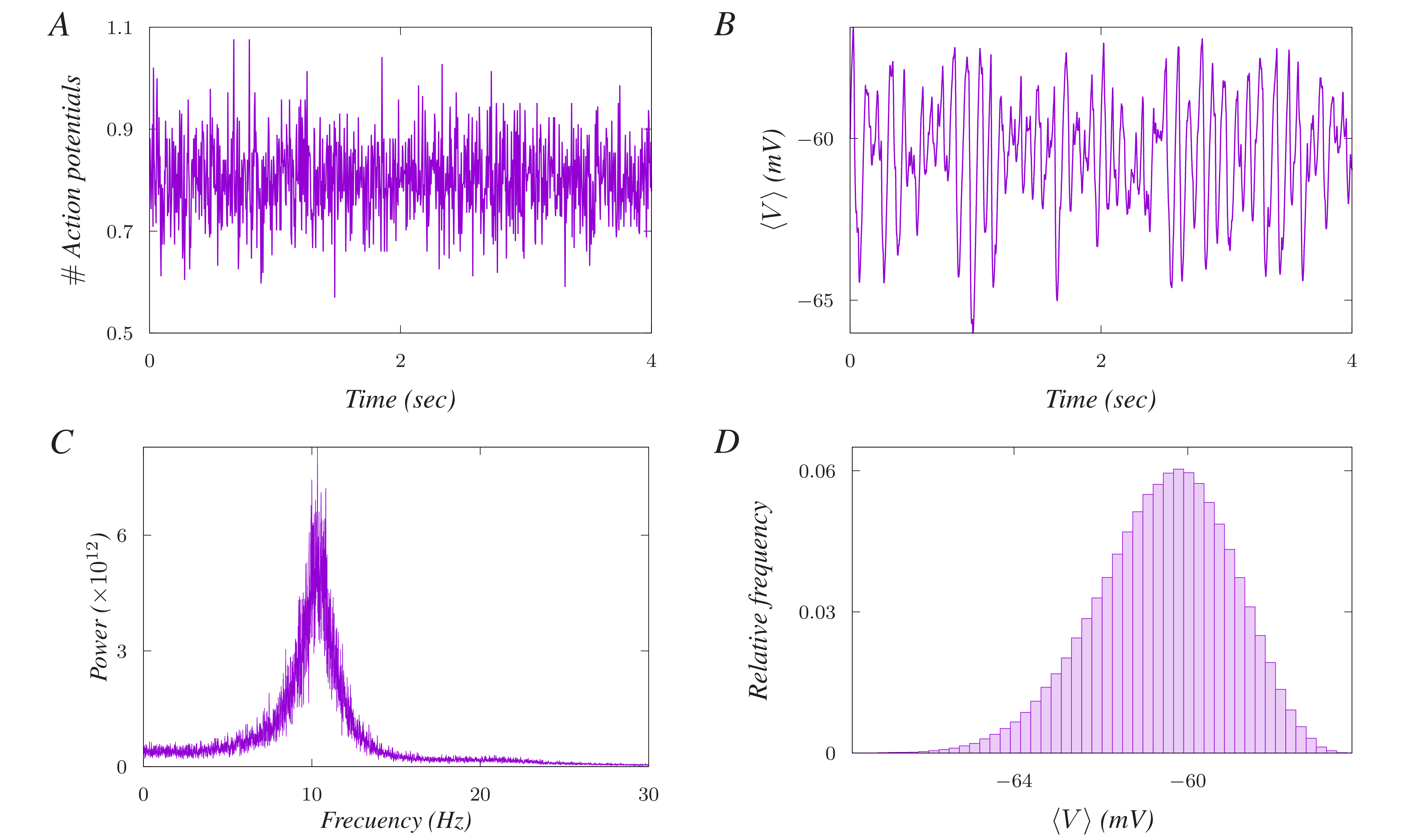
Figure 2: (A) Example of the noisy time series that each E neuron receives on the average from $n=100$ external E neurons from outside the network. This has a Poisson distribution of mean $\mu=0.8$. In practice, we compute the number of external action potentials each E neuron receives each time step $t_{i}=i\Delta t$ from such distribution, and add this number to the number of depolarization waves in the sum appearing in (8). (B) Emergent output as measured by the average membrane potential of all the E neurons. Its statistical features are shown in panels (C), depicting the sharp power spectral density, and (D), the corresponding probability distribution.

Results

We monitored several dynamic variables during the network evolution with time, including: (a) the sum of membrane potentials of E neurons; (b) the same for I neurons; and (c) the action potentials density leaving the network via axons, i.e., the mean firing rate associated to the Es, i.e, $\nu(t)=(1/N_{E})\sum_{i=1}^{N_{E}}s_{i}^{E}(t)$ where $s_{i}^{E}(t)=1,0$ if the $E$ neuron is firing or not at time $t.$ Since the number of Es is dominant, we identify (a) with the EEG signal which, therefore, is assumed to be the extracellular replica of the membrane time variation. This is a sensible assumption since EEG experiments are expected to record at a site on the scalp the summed electrical field potentials from all cortical neurons in a certain volume of tissue under the electrode. The fact is that a control of these quantities shows that the model steady state is quickly attained —typically in around 100$\Delta t$ steps during our studies— from any initial condition.

Consider first the case in which $V_{\text{ext}}=V_{0}=0$ so that the only input in Eq.(1) besides $V_{\text{in}}$ is $V_{\text{noise}}.$ When this is implemented as a Poisson distribution, our system responds, as illustrated in Fig. 2, with a well-defined rhythm wave, in spite of the wide range of frequencies in the input, in agreement with experiments. That is, for a sufficiently large input mean ($\mu=0.8$ in the example of Fig. 2) the two populations (E and I) of neurons show coupled oscillations producing collective coherent resonance, and the familiar $\alpha$-rhythm emerges. This is revealed, for instance, by the power spectral density of the time series for the average membrane potential over all E neurons, which shows a well-defined peak around $10.5$ Hz in Fig. 2.

There are indications that the same simple model may generate other types of rhythms as one varies the parameter $\mu.$ Would this be the case, it would generalize our last observation, already reported in [8], along an important path as it would indicate that all the familiar brain-rhythms may be considered as noise filtered by the networked system. As a matter of fact, decreasing $\mu$ we observe that the coupling between the two populations of neurons which induces the coherent rhythm tends to get worse. For instance, the time series of the mean membrane potential for $\mu=0.6$ do not have the well defined periodicity nor, therefore, the acute peak in the power spectral density in Fig. 2C. We shall demonstrate below that such lack of periodicity for $\mu\sim 0.6$ corresponds to a phase transition between an asynchronous condition and a synchronous one. This fact does not show up in [8] where a (one hundred times) larger time discretization artificially increases synchronicity —the same also obscures other important facts concerning larger values of $\mu,$ as we shall illustrate below.

Figure 3: Some characteristics of the different dynamical phases that emerge as $\mu$ is varied. Panel A shows the (linear) adiabatic temporal variation of $\mu$ during the experiment, from $\mu=0.1$ increasing by a factor $1.00002$ every time unit $\Delta t$. The resulting dynamic behaviour is illustrated in panel B showing $V\left(t\right),$ and this is detailed in panel C (right) for constant $\mu$ (=0.2, 0.9, 10 and 17, respectively) within the four regions of different behavior. Note how oscillations are too weak for $\mu\lesssim 0.5$ (phase I) to speak about actual coherence resonance, while they are clear for $\mu\gtrsim 0.6,$ and coupling is observed best arround $\mu=1.5$. Thereafter, coherence begins to decrease and the the synchronization between the E and I populations decreases. Between $\mu\approx 5$ and $\mu\approx 15$ there is an asynchronous phase (III) in which frecuency cannot be defined. However, coherence and synchrony are restored and the frecuency is well-defined again for $\mu\gtrsim 15$ (phase IV).

The new circumstance uncovered here suggested us using $\mu$ as a control parameter, and thus explore further the emergence of brain rhythms, which then happen to surface as characteristics of dynamic phases. Fig.3 partially illustrates the varied collective behavior that shows up as $\mu$ is increased adiabatically in time. This reveals that, following a rather disordered phase (I) for $\mu\lesssim 0.5,$ oscillations become well defined (phase II) after $\mu\approx 0.6.$ As $\mu$ is increased further, coherence is observed to decrease, as well as the synchrony among E and I populations —in particular, we observe that E neurons are first triggered simultaneously, which induces firing of Is at the same frequency but after a certain time lag. Asynchrony then sets in from $\mu\approx 5$ to $\mu\approx 15$ (phase III), with no collective well-defined frequency. However, coherence and synchrony with a clear frequency are restored for $\mu\gtrsim 15$ (phase IV) until $\mu>25,$ when the noise is so high that it looses any biological meaning.

To confirm these —non-equilibrium but thermodynamic-like [9]— phases, instead of slowly varying $\mu$ we also maintained the noise constant during each simulation. Repeating this operation for different noise values of $\mu,$ we obtained the graphs in Fig.3 which happen to illustrate different types of behavior. In summary, we may define:

Phase I,

$\mu\lesssim 0.5:$ asynchrony with low activity. The two subpopulations of neurons act almost uncoupled. No well-defined oscillation frequency.

Phase II,

$0.6\lesssim\mu\lesssim 5:$ synchrony with broad collective oscillations of the two subpopulations, which then oscillate coupled at a well-defined frequency.

Phase III,

$5\lesssim\mu\lesssim 15:$ high activity with lost of the overall coherence. Ups and downs in the average membrane potentials of the two subpopulations are such that the excitation does not “wait” for the end of the inhibition in every period and vice-versa, so that the periodicity and rhythm that characterize phase II is now lost.

Phase IV,

$\mu\gtrsim 15:$ synchrony, namely, the Es are triggered almost simultaneously, and the same with the Is. This is because the threshold is exceeded again in a short time (after each firing event and its subsequent refractory period) which facilitates synchronicity (and reduces the possibility of other type of behavior). This synchrony goes with oscillations of the average membrane potential with an amplitude lower than in phase II but is more regular than these and shows a well defined oscillation frequency, as revealed by the power spectrum.

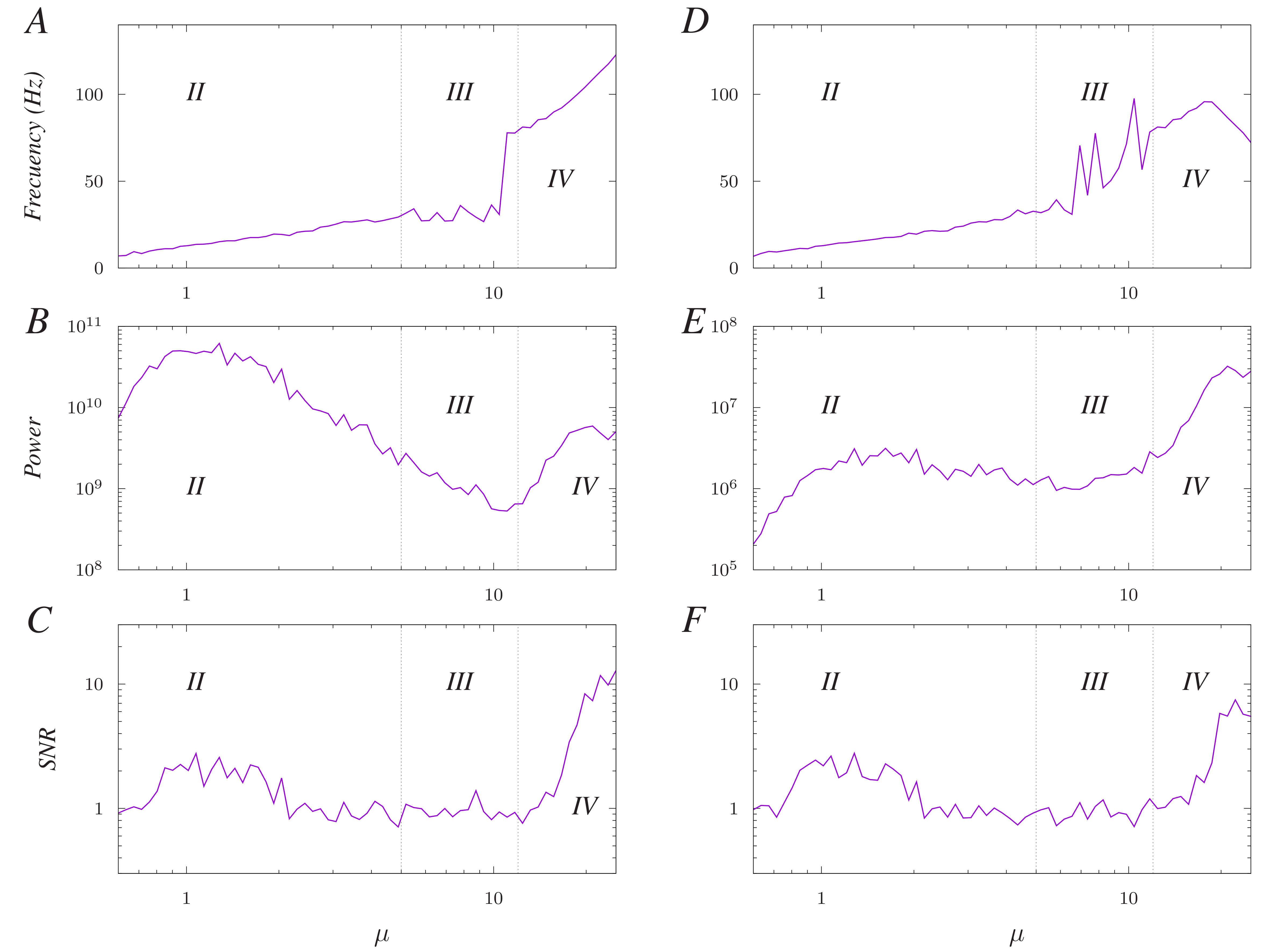
Figure 4: Panel A: Frequency at the power spectra peak of time series for the mean membrane potential as a function of $\mu$ for $I_{0}=0$. There is asynchrony for $5\lesssim\mu\lesssim 15$ (phase III) and regions of coherent resonance before $\mu\approx 5$ (phase II) and after $\mu\approx 15$ (phase IV). Panel B: The height of the peak in A, which is highest for phases (II and IV) due to coherent resonance. Panel C: Signal-to-noise ratio (SNR). The highest values occur again for phases II and IV, and the minimum ones during the asynchronous phases (I and III). Panels D, E and F: Same as in panels A, B and C, respectively, but for the time series of the mean firing rate of the E neurons, which confirm the results on the left.

It ensues that the familiar brain rhythms, namely, $\alpha,$ $\beta,$ $\gamma$ and ultrafast oscillations in EEG recordings from actual awake brains, have a well-defined correspondence with these rhythmic oscillations of the average membrane potential in the model. To clearly uncover this, we performed extra runs lasting $2^{18}$ time steps (equivalent to $10.5$ s) for each of the 66 $\mu$ values in a geometric progression starting at $\mu=0.5.$ From such time series, we collected both the average membrane potential and the mean firing rate of the E population, then computed the power spectra, and searched for a maximum on each of them. Our main results are summarized in Fig.4 where panel A depicts the frequency at which this peak occurs as a function of $\mu.$ There is no evidence of any well defined frequency for $\mu\lesssim 0.5$ (phase I, not shown), nor for $5\lesssim\mu\lesssim 15$ (phase III) which shows abrupt jumps. However, during the intermediate region (phase II), the frequency increases from $6\,Hz$ to $25\,Hz$ —thus describing the spectrum of $\alpha,$ $\beta$ and $\gamma$ waves— and, finally (phase IV), this goes from $80\,Hz$ to $130\,Hz$ —corresponding to high $\gamma$ and ultrafast oscillations. The same is confirmed by time series for the mean firing of E neurons in Fig.4D. This picture becomes even more coherent and interesting when one realizes, as it turns out to be the case, and we develop it below, that the passage from one behavior to a contiguous qualitatively-different one is throughout a non-equilibrium phase transition. The system in this way exhibits varied behavior with quite efficient features and great economy [4].

On the other hand, the peaks in Fig.4B are higher in the presence of coherent resonance, i.e., phases II and IV, than during the asynchronous phases I (not shown since not a clear peak develops in fact here) and III. The behavior is similar for the mean firing rate in Fig.4E. It also interests the $\mu$ variation of the signal-to-noise ratio (SNR) at the power spectra peak, i.e., its height divided by the average in a small range around. Even more clear than the spectra peaks, the SNR shows maxima if coherence occurs (II and IV) and goes to minima in the asynchronous phases (I and III). The same is confirmed by the power spectrum of the time series for both the membrane potential in Fig.4C and the mean firing rate in Fig.4F. Specifically, the maximum coherence value is achieved in both cases around $\mu\simeq 1.3$ (within phase II) and for $\mu\gtrsim 20$ (within phase IV), and it is also noticeable that the SNR maximum, for both the global membrane potential and the mean firing rate, is higher for phase IV than for phase II.

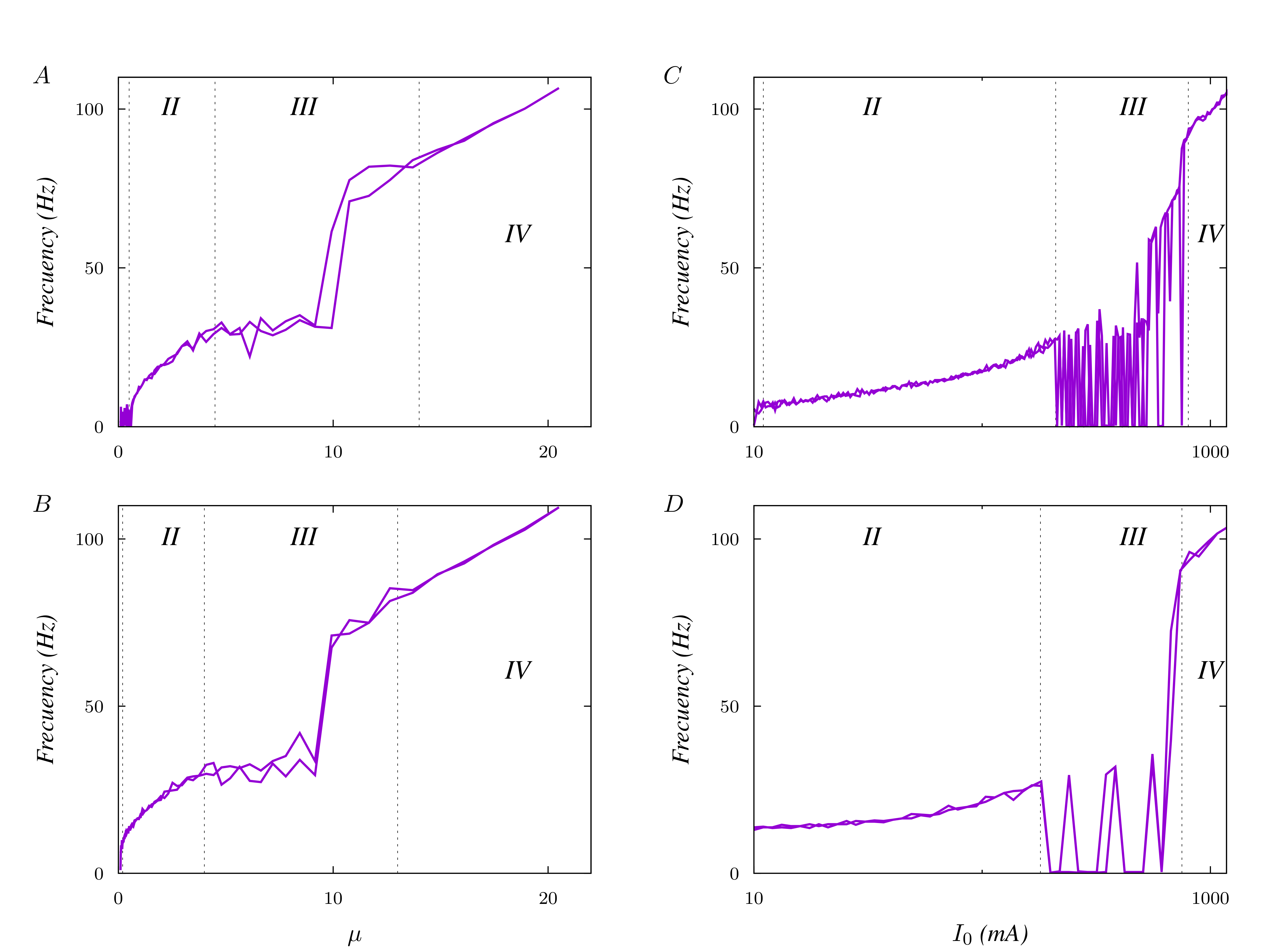
Figure 5: Study of hysteresis as a function of $\mu$ (left) and $I_{0}$ (right). Panel A: Frequency at which the peak of the power spectra for the mean membrane potential occurs (as $\mu$ is increased and decreased adiabatically with $I_{0}=0$). The two curves superimpose where the frequency is well defined. Panel B: The same but for $I_{0}=50,$ confirming the phases in A, but shifted to the left. Panel C: The frequency in A but as a function of the constant input $I_{0}$ for $\mu=0.5,$ which confirms the same phases and shows that $210\leqslant I_{0}\leqslant 750$ is an asynchronous region in which frequency is not well-defined. Panel D: Same as in panel C but for $\mu=1$ showing the same but with changes now shifted to the left relative to panel C because $\mu$ is now higher.

The above suggests a great interest in characterizing the transition regions separating qualitatively different behaviors as one varies $\mu$ and $I_{0}.$ Particularly, there is interest in the transition between phases III and IV. Fig.4A, for instance, reveals that this is sharp, suggesting a thermodynamic-like discontinuous phase transition. To address this, we run our system during 10s for each $\mu$ value, as we varied adiabatically this parameter in geometric progression while keeping $I_{0}=0.$ We retained the final state of all the neurons in each run to serve as the initial state for the run at the next noise value, which only differs in a small percentage from the previous one. Once the maximum $\mu$ is reached, the process is reverted, keeping again each final state as the initial one during this noise reduction process. The resulting hysteresis cycle around transitions III$\leftrightarrow$IV is shown in Fig.5A, which confirms the discontinuous first-order-like nature of the phase transition. Such (even small) hysteresis seems to reflect that the frequency of the global oscillations is not well-defined in phase III; in fact, this shows no clear peak in the power spectra, and the maximum we use to compute hysteresis can depend on the run conditions. However, when the frequency is well-defined, the round-trip curves superimpose. We obtain similar results for $I_{0}=50$ in Fig.5B, but with the phase changes somewhat shifted to the left.

The fact that our model shows the same qualitative behavior or phases within a wide ample range of $I_{0}$ values suggests that its behavior is robust to the type of input, and we confirmed this by moving $I_{0}$ adiabatically for $\mu=0.5$ (Fig.5C) and $\mu=1$ (Fig.5D). Note that phase I is not shown, since for $\mu=1$ the system is at phase II even for $I_{0}=10,$ that phase III occurs for $180\leq I_{0}\leq 700$ and that, as expected, the phase changes are shifted to the left relative to Fig.5C because $\mu$ is now higher. The conclusion is that the system is sensible to the total current arriving to the network but not to the type of input. In other words, increasing the noise and $I_{0}$ tends to increases the excitability of both neuron populations but the emergent behavior is rather due to the complex interplay between the activity of E and I populations.

Stochastic resonance as a detector of phase transitions in EEG activity

We also checked the case of a weak input $V_{\text{ext}}=d\,\sin(2\pi ft)$ with small $d$ to the neural network, instead of $V_{\text{ext}}=0$ as above. In general, even relatively small values of $d$ induce a new maximum at frequency $f$ in the power spectra, as shown in Fig.6 (right column).

Figure 6: Case of $\mu=10$ showing the effect of adding (right column) a small signal $V_{\text{ext}}=d\,\sin 2\pi f\,t$ to each $E$ neuron. The left column is for $d=0$ while the right one is for $d=25$ and $f=40\,Hz$. Top panels show the mean membrane potential of E (violet line) and I (green line) neurons with (panel E) and without (panel A) the external signal. Panels B and F depict the corresponding (membrane potential) power spectra for the I neurons in both situations, and panels C and G show the same for E neurons. At the bottom, panels D and H illustrate the corresponding power spectra of the mean firing rate for E neurons. The signal only slightly modifies dynamics but a clear peak emerges at frequency $f$.

The emergent peak here —which happens to stand out more or less depending on the values for $d$ and $\mu$— reveals the existence of the so-called stochastic resonance (SR) phenomenon [10]. That is, the propagation of a weak signal is enhanced at certain intermediate level of noise while it is generally obscured at lower and higher levels of noise. The SNR in the power spectra consequently increases at those moderate values of the noise. As it was already shown [3], this is just a consequence of the great susceptibility the cooperative system exhibits in a region in which a phase transition occurs, so that it provides a simple method to detect changes of qualitative behavior in these types of systems.

Figure 7: Emergence of stochastic resonance in the system in figure 1, for $I_{0}=0,$ when a weak sinusoidal input $V_{\text{ext}}$ of low frequency ($f\sim 4Hz$) (left graph) and high frequency ($f\sim 40Hz$) (right graph) affects each $E$ neuron. SR peaks appear around the phase transition points (vertical dashed lines at $\mu=0.6,\,6$ and $16$) depicted in the top panels. Note in the left graph that the jump corresponding to the change of behaviour in simulations between phases IV and III (see top panel) appears around $\mu\approx 10$ (see red vertical dashed line) that coincides with the larger resonance peak for large level of noise. Secondary resonance peaks occurs around this maximun for $\mu\approx 6$ and $16.$ In the right panel, however, such maximun does not show. Also, the low noise resonance peaks around $\mu\approx 0.6$ is neither appearing and the only ones are those around $\mu\approx 6$ (poorly seeing) and $16$ (very clearly depicted). Different SNR curves here were obtained after averaging over 100 trials and computing the power spectra over a time series of $2^{18}ms$ for each trial.

A general evidence of SR phenomena in the system is illustrated in Fig.7 for $I_{0}=0,$ showing the signal to noise ratio ($SNR$) as a function of the noise level $\mu$ for both low-frequency ($\sim 4Hz$) and high-frequency ($\sim 40Hz$) inputs signals. In agreement with the interpretation of stochastic resonance in [3], here we observe how SR peaks develop around the phase transitions described above. For low-frequency signals (left graph) there are clear maximum at $\mu\approx 0.6,$ $6$ and $16$ corresponding to the phase transitions I$\leftrightarrow$II, II$\leftrightarrow$III and III$\leftrightarrow$IV, respectively. The $SNR$ also shows a peak for $\mu\approx 10$ which corresponds to the level of noise at which finite-size jumps between III$\leftrightarrow$IV occurs in simulations. The emergence of this peak can be explained assuming that noise makes that these finite-size jumps of activity between both phases can be driven by the weak stimulus, so an amplification of the weak signal occurs at such noise level. Then, we expect that such peak will disappear as the network size is increased which will be an indication that the transition III$\leftrightarrow$IV is of first-order type as simulations seams to indicate (see top graphs in Fig. 7). For high-frequency signals ($\sim 40Hz$), only the transitions II$\leftrightarrow$III and III$\leftrightarrow$IV are clearly marked by stochastic resonance peaks around $\mu\approx 6$ and $16,$ the first hardly distinguishable and the last one very clear. The peak around $\mu\approx 0.6$ is not appearing due to the fact that system oscillations at such level of noise at a natural frequency of alpha range around $10Hz$ or less, which is very small compared with the weak signal stimulation frequency ($40Hz$). This is incompatible with the emergence of the SR where the stimulation frequency must be very low compared with the intrinsic oscillation frequency of the system. Note that this impediment does not occur for the the resonance peak around $\mu=17$ since for this case the intrinsic oscillation frequency of the system is around $75Hz$ or larger which is bigger that the stimulation frequency of $40Hz$, so conditions for the emergence of SR still hold. The transition II$\leftrightarrow$III occur around $\mu\approx 0.6$ with system oscillations of frequency around the stimulation frequency, so this is the reason why the SR peak around $\mu\approx 0.6$ is not so clearly depicted. Also remarkable in this high-frequency stimulation case is the presence of an additional resonance peak around $\mu\approx 2.5$ (marked with “*” in the figure) which corresponds with a range of frequencies$\sim 25-30$$Hz$, and it could indicate the exact limit between $\beta$ (with intrinsic frequency between $12$ to $30Hz$) and $\gamma$ brain waves (with intrinsic frequency larger than $30Hz$) as experimental psychologists and neuroscientists have widely described (see for instance [23, 24, 25]). This overall behaviour should also be discernible in actual EEG experiments.

Discussion

We here present an extension, and formalization according to recent familiar standards, of a model for the generation of brain $\alpha$ rhythms [8] which provides a simple and well-defined scenario also for other types of brain waves. In addition to signals from other neurons $\left(V_{\text{in}}\right),$ and from outside the network —which are globally portrayed here as a Poisson noise $\left(V_{\text{noise}}\right)$ which is characterized by the parameter $\mu$— our model Eq.(1) includes a constant current $I_{0}$ and a small external input signal $V_{\text{ext}}$. Our main findings may be summarized as follows:

• Previous results [8] are confirmed and, using realistic, smaller time steps, we describe lower degrees of coherence and real levels of synchronicity.

• In this way, we identify four different “phases” or qualitative types of dynamic behavior in the model. As $\mu$ is increased, this exhibits oscillations that are too weak in amplitude so that any coherence is precluded (phase I), coherent resonance and synchrony (phase II), asynchrony showing abrupt jumps in the corresponding frequency curves (phase III), and coherence and synchrony with a well-defined frequency again (phase IV).

• In phase II, our system precisely includes the frequency spectrum of $\alpha,$ $\beta$ and low $\gamma$ waves of actual EEG recordings, and phase IV covers the frequencies corresponding to high $\gamma$ and ultrafast oscillations.

• The highest coherent resonance, as revealed by the power spectra peak and the corresponding SNR, is for phases II and IV, while the lowest one occurs in the asynchronous phases I and III.

• The average amount of electrical impulses arriving to the network per unit of time —that we parametrize as $\mu$— is essential to characterize the different phases, more than the nature, either constant or noisy, of the input.

• Stochastic resonance [3, 4] is revealed, e.g., by SNR, locating changes of qualitative behavior when the system receives a signal. We confirm that this fact may provide a powerful tool to investigate phase transitions in mammals’ and other brains using simple techniques such as EEG recordings or simple experiments as devised in [3].

The above picture indicates, on one hand, that a single mechanism is behind the familiar brain rhythms and, on the other, that such waves are related to the general phenomena of non-equilibrium phase transitions, where a system is known to be highly susceptible, efficient and adaptable [9, 4]. This is compatible with specific mechanisms that might act during the generation of brain oscillations while cognitive functions occur. However, a one-to-one correspondence between different type of brain oscillations and cognitive functions cannot be stablished in fact, there are many more different cognitive processes than types of brain waves [26]. It seems sensible to assume that similar brain waves in the same frequency band can contribute to different cognitive functions depending on the particular brain area in which they originated and on their particular temporal features [26]. For example [27], while local synchronization during visual processing evolves in the $\gamma$ range, synchronization between neighboring temporal and parietal cortex during multi-modal semantic processing may evolve in a lower $\beta$ (12-18 Hz) range, and long range fronto-parietal interactions during working memory retention and mental imagery in the $\theta$ (4-8 Hz) and $\alpha$ (8-12 Hz) ranges. That is, a relationship may exist between functional integration and synchronization frequency which could be due to conduction delays in long corticortical axons —up to several tens of ms for conduction distances of $\sim$10 mm— and convert $\gamma$ to $\beta$ oscillations (with cycle times ranging from $30$ to $70$ ms). The same process for more widely-dispersed interactions could produce activity in the active cortex in the $\alpha$ range (cycle time 77–125 ms) or even in the $\theta$ range. To our knowledge, however, these details have yet been poorly demonstrated and the argument requires that all axonal connections of a given network were approximately the same length, which is a too strong assumption for regions of arbitrary extension. In addition, electrical stimulation of V1 induces enhanced $\gamma$-band activity in V4, whereas V4 stimulation induces enhanced $\alpha\mbox{{-}}\beta$-band activity in V1 [28], when it is supossed that the conduction delays are aproximately the same from V1 to V4 than from V4 to V1. Recognizing that the presence of conduction delays may importantly complicate the network dynamics [29], and that brain oscillations could be related to many body oscillations [30] – as heart rate, heart rate variability, breathing frequencies, fluctuations in the BOLD signal, and others – our proposal does not require any hypothesis concerning conduction times or too speculative assumptions concerning the coupling of the brain activity with any type of body oscillations. From a different point of view, given the modular structure of the brain [31], we may imagine small networks with a great internal connectivity, each as ours here and perhaps in some of the dynamic phases we have described subject to an input. Furthermore, it is sensible to assume that, in a large region of interconnected neurons, an input from other modules will not affect all the neurons, since otherwise it might induce an anomalous high physiological level of activity. On the average, one should expect our parameter $\mu$ to be low and only high inputs eventually reaching small local regions. Within this scenario, our model suggests that large synchronized regions receive small inputs, and therefore will oscillate in the $\alpha$ regime, while small local synchronized regions receiving a large input will oscillate synchronously in the $\gamma$ range. Our scenario is thus compatible with the one in [32].

Also, we mention that some authors associate consciousness with coherent $\gamma$ oscillations in different parts of the brain, and thus explain episodes of attention [33]. In the light of our results, we can hypothesize that the transition III$\rightarrow$IV could be related to the emergence of awareness of memories associated with the modules that reach the corresponding input, a hyphothesis that could be tested experimentally. In fact, we could include all the 40-70 Hz frequencies in phase IV choosing adequately model parameter values. In particular, our network model may easily involve a small random delay of small variance in all the connections, a topology different that the one in Fig.1A, and/or vary the parameters of the EPSP and IPSP waves in Fig.1B to achieve this. Other theories of consciousness, as the Integrated Information Theory [34] and its continuous dynamical system version [35] are also consistent with our scenario in which one may have two phases with very different levels of activity, both with a synchronicity that facilitates the communication with other mechanisms, and our phases II and IV would be equivalent to the “off” and “on” states in this theory.

Finally, our findings here can also be useful to design appropriate deep learning algorithms based on SR [12, 13] which might optimally learn feature representation in the presence of noise in actual EEG recordings, or to identify phase transitions in the brain from raw data in EEG time series [11]

References

- [1] V. M. Eguiluz, D. R. Chialvo, G. A. Cecchi, M. Baliki, and A. V. Apkarian. Scale-free brain functional networks. Phys. Rev. Lett., 94:018102, 2005.
- [2] J. Hesse and T. Gross. Self-organized criticality as a fundamental property of neural systems. Frontiers in Systems Neuroscience, 8:166, 2014.
- [3] J. J. Torres and J. Marro. Brain performance versus phase transitions. Scientific Reports, 5:12216 EP –, 2015.
- [4] J. Marro and D. R. Chialvo, La Mente es Crítica — Descubriendo la admirable complejidad del cerebro, EUG (University of Granada Press), Granada 2017 (an English new version of the contents of this book is now in progress).
- [5] M. A . Muñoz, Colloquium: Criticality and dynamical scaling in living systems, Review of Modern Physics. 90(3), 031001, 2018.
- [6] L. Cocchi, L. L. Gollo, A. Zalesky, M. Breakspear. Criticality in the brain: A synthesis of neurobiology, models and cognition. Progress in Neurobiology, 158, 132-152, 2017.
- [7] L. L. Gollo. Coexistence of critical sensitivity and subcritical specificity can yield optimal population coding. Journal of The Royal Society, Interface, 14 (134), 2017.
- [8] F. H. Lopes da Silva, A. Hoeks, H. Smits, and L. H. Zetterberg. Model of brain rhythmic activity. Kybernetik, 15(1):27–37, 1974.
- [9] J. Marro and R. Dickman, Nonequilibrium Phase Transitions in Lattice Models, Cambridge University Press, Cambridge 2005.
- [10] L. Gammaitoni, P. Hänggi, P. Jung, and F. Marchesoni. Stochastic resonance. Review of Modern Physics., 70:223–287, Jan 1998.
- [11] W. Zhang, J. Liu, T.-Ch. Wei Machine learning of phase transitions in the percolation and XY models. arXiv:1804.02709v1, 2018.
- [12] S. Ikemoto ; F. Dalla-Libera ; K. Hosoda, Stochastic resonance induced continuous activation functions in a neural network consisting of threshold elements 2016 International Joint Conference on Neural Networks (IJCNN), IEEE publisher, pp 2603–2608, 2016
- [13] Y. Roy, H. Banville, I. Albuquerque, A. Gramfort, T. H. Falk, J. Faubert. Deep learning-based electroencephalography analysis: a systematic review. arXiv:1901.05498v2, 2019.
- [14] T. Tömböl. Short neurons and their synaptic relations in the specific thalamic nuclei. Brain Research, 3(4):307–26, 1967.
- [15] V. Braitenberg and A. Schüz. Cortex: Statistics and Geometry of Neuronal Connectivity. Springer, 1998.
- [16] H. Markram, M. Toledo-Rodriguez, Y. Wang, A. Gupta, G. Silberberg, and C. Wu. Interneurons of the neocortical inhibitory system. Nature Review of Neuroscience, 5(10):793–807, Dec 2004.
- [17] M. Okun and I. Lampl. Balance of excitation and inhibition. Scholarpedia, 4(8):7467, 2009.
- [18] L. F. Abbott. Lapicque’s introduction of the integrate-and-fire model neuron (1907). Brain Research Bulletin, 50(5-6):303–304, 1999.
- [19] E. R. Kandel, J.H. Schwartz, and T. M. Jessell. Principles of Neural Science. McGraw-Hill, 4th edition, 2000.
- [20] W. R. Levick and W. O. Williams. Maintained activity of lateral geniculate neurones in darkness. J Physiology, 170:582–597, 1964.
- [21] J. M. Fuster, A. Herz, and O. D. Creutzfeldt. Interval analysis of cell discharge in spontaneous and optically modulated activity in the visual system. Archives Italiennes de Biologie, 103(1):159–177, 1965.
- [22] Ch. Koch. Biophysics of Computation: Information Processing in Single Neurons. Oxford University Press, 1999.
- [23] R. E. Dustman, R. S. Boswell, P. B. Porter. Beta Brain Waves as an Index of Alertness. Science 137(3529): 533–534, 1962.
- [24] G. Buzsáki. Rhythms of the Brain. New York: Oxford University Press. p. 4. 2006.
- [25] J. D. Kropotov. Beta Rhythms. In: Quantitative EEG, Event-Related Potentials and Neurotherapy, Academic Press, San Diego, 2009, Pages 59–76 2009.
- [26] C.S. Herrmann, D. Strüber D, R.F. Helfrich, A.K. Engel. EEG oscillations: from correlation to causality. International Journal of Psychophysiology, 103: 12–21, 2016.
- [27] R. Miller. Theory of the normal waking eeg: From single neurones to waveforms in the alpha, beta and gamma frequency ranges. International Journal of Psychophysiology, 64(1):18 – 23, 2007.
- [28] G. Michalareas, J. Vezoli, S. Pelt, J. Schoffelen, H. Kennedy, P. Fries. Alpha-beta and gamma rhythms subserve feedback and feedforward influences among human visual cortical areas. Neuron 89: 384–397, 2016.
- [29] W. S. Lee, E. Ott, and T. M. Antonsen. Large coupled oscillator systems with heterogeneous interaction delays. Physical Review Letters, 103:044101, Jul 2009.
- [30] W. Klimesch The Frequency Architecture of Brain and Brain-Body Oscillations: An Analysis. European Journal of Neuroscience, 48(7): 2431–2453, 2018.
- [31] E. Bullmore and O. Sporns. Complex brain networks: graph theoretical analysis of structural and functional systems. Nature Reviews of Neuroscience, 10(3):186 –198, 2009.
- [32] A. von Stein and J. Sarnthein. Different frequencies for different scales of cortical integration: from local gamma to long range alpha/theta synchronization. International journal of psychophysiology , 38(3):301–13, 2000.
- [33] F, Crick and Ch. Koch. Towards a neurobiological theory of consciousness. Seminars in the neurosciences, 2:263 – 275, 1990.
- [34] M. Oizumi, L. Albantakis, and G. Tononi. From the phenomenology to the mechanisms of consciousness: Integrated information theory 3.0. PLoS Computational Biology, 10(5):1–25, 05, 2014.
- [35] F. J. Esteban, J. A. Galadí, J. A. Langa, J. R. Portillo, and F. Soler-Toscano. Informational structures: A dynamical system approach for integrated information. PLoS Computational Biology, 14(9): , 2018.