Complementary Learning for Overcoming Catastrophic Forgetting Using Experience Replay

Abstract

Despite huge success, deep networks are unable to learn effectively in sequential multitask learning settings as they forget the past learned tasks after learning new tasks. Inspired from complementary learning systems theory, we address this challenge by learning a generative model that couples the current task to the past learned tasks through a discriminative embedding space. We learn an abstract level generative distribution in the embedding which allows generation of data points to represent past experience. We sample from this distribution and utilize experience replay to avoid forgetting and simultaneously accumulate new knowledge to the abstract distribution in order to couple the current task with past experience. We demonstrate theoretically and empirically that our framework learns a distribution in the embedding, which is shared across all task, and as a result tackles catastrophic forgetting.

1 Introduction

Recent breakthrough of deep learning has led to algorithms with human-level performance for many machine learning applications. This may seem natural as these networks are the best accessible tools that mimic human nervous system Morgenstern et al. (2014). However, this success is highly limited to single task learning, and retaining learned knowledge in a continual learning setting remains a major challenge. That is, when a deep network is trained on multiple sequential tasks with diverse distributions, the new obtained knowledge usually interferes with past learned knowledge. As a result, the network often is unable to accumulate the new learned knowledge in a manner consistent with the past experience and forgets past learned tasks by the time the new task is learned. This phenomenon is called “catastrophic forgetting” in the literature French (1999). This phenomenon is in contrast with continual learning ability of humans over their lifetime.

To mitigate catastrophic forgetting, a main approach is to rely on replaying data points from past tasks that are stored selectively in a memory buffer Robins (1995). This is inspired from the Complementary Learning Systems (CLS) theory McClelland et al. (1995). CLS theory hypothesizes that a dual long-term and short-term memory system, involving the neocortex and the hippocampus, is necessary for continual lifelong learning ability of humans. In particular, the hippocampus rapidly encodes recent experiences as a short-term memory that is used to consolidate the knowledge in the slower neocortex as long-term memory through experience replays during sleep/conscious recalls Diekelmann and Born (2010). Similarly, if we selectively store samples from past tasks in a buffer, like in the neocortex, these samples can be replayed to the deep network in parallel with current task samples from recent-memory hippocampal storage to train the deep network jointly on past and current experiences. In other words, the online sequential learning problem is recast as an offline multitask learning problem that guarantees learning all tasks. A major issue with this approach is that the memory size grows as more tasks are learned and storing tasks’ data points and updating the replaying process becomes more complex. Building upon recent successes of generative models Goodfellow et al. (2014), this challenge has been addressed by amending the network structure such that it can generate pseudo-data points for the past learned tasks without storing data points Shin et al. (2017).

In this paper, our goal is to address catastrophic forgetting via coupling sequential tasks in a latent embedding space. We model this space as output space of a deep encoder, which is between the input and the output layers of a deep classifier. Representations in this embedding space can be thought of neocortex representations in the brain, which capture learned knowledge. To consolidate knowledge, we minimize the discrepancy between the distributions of all tasks in the embedding space. In order to mimic the offline memory replay process in the sleeping brain Rasch and Born (2013), we amend the deep encoder with a decoder network to make the classifier network generative. The resulting autoencoding pathways can be thought of neocortical areas, which encodes and remembers past experiences. We fit a parametric distribution in the embedding space into the empirical distribution of data representations. This distribution can be used to generate pseudo-data points through sampling, followed by passing the samples into the decoder network. The pseudo-data points can then be used for experience replay of the previous tasks towards incorporation of new knowledge. This would enforce the embedding to be invariant with respect to the tasks as more tasks are learned, i.e., the network would retain the past learned knowledge as more tasks are learned.

2 Related Work

Past works have addressed catastrophic forgetting using two main approaches: model consolidation Kirkpatrick et al. (2017) and experience replay Robins (1995). Both approaches implement a notion of memory to enable a network to remember the distributions of past learned tasks.

The idea of model consolidation is based upon separating the information pathway for different tasks in the network such that new experiences do not interfere with past learned knowledge. This idea is inspired from the notion of structural plasticity Lamprecht and LeDoux (2004). During learning a task, important weight parameters for that task are identified and are consolidated when future tasks are learned. As a result, the new tasks are learned through free pathways in the network; i.e., the weights that are important to retain knowledge about distributions of past tasks mostly remain unchanged. Several methods exist for identifying important weight parameters. Elastic Weight Consolidation (EWC) models posterior distribution of weights of a given network as a Gaussian distribution which is centered around the weight values from last learned past tasks and a precision matrix, defined as the Fisher information matrix of all network weights. The weights then are consolidated according to their importance, i.e., the value of Fisher coefficient Kirkpatrick et al. (2017). In contrast to EWC, Zenke et al. Zenke et al. (2017) consolidate weights in an online scheme during learning a task. If a network weight contributes considerably to changes in the network loss, it is identified as an important weight. More recently, Aljundi et al. Aljundi et al. (2018) use a semi-Hebbian learning procedure to compute the importance of the weight parameters in a both unsupervised and online scheme. The issue with the methods based on structural plasticity is that the network learning capacity is compromised to avoid catastrophic forgetting. As a result, the learning ability of the network decreases as more tasks are learned.

Methods that use experience replay, use CLS theory to retain the past tasks’ distributions via replaying selected representative samples of past tasks continuously. Prior works mostly have investigated on how to store a subset of past experiences to reduce dependence on memory. These samples can be selected in different ways. Schaul et al. select samples such that the effect of uncommon samples in the experience is maximized Schaul et al. (2016). Isele and Cosgun explore four potential strategies to select more helpful samples in a buffer for replay Isele and Cosgun (2018). The downside is that storing samples requires memory and selection becomes more complex as more tasks are learned. To reduce dependence on a memory buffer similar to humans French (1999), Shin et al. Shin et al. (2017) developed a more efficient alternative by considering a generative model that can produce pseudo-data points of past tasks to avoid storing real data points. They use a generative adversarial structures to learn the tasks distributions to allow for generating pseudo-data points without storing data. However, adversarial learning is known to require deliberate architecture design and selection of hyper-parameters Roth et al. (2017), and can suffer from mode collapse Srivastava et al. (2017). Alternatively, we demonstrate that a simple autoencoder structure can be used as the base generative model. Our contribution is to match the distributions of the tasks in the middle layer of the autoencoder and learn a shared distribution across the tasks to couple them. The shared distribution is then used to generate samples for experience replay to avoid forgetting. We demonstrate effectiveness of our approach theoretically and empirically validate our method on benchmark tasks that has been used in the literature.

3 Generative Continual Learning

We consider a lifelong learning setting Chen and Liu (2016), where a learning agent faces multiple, consecutive tasks $\{\mathcal{Z}^{(t)}\}_{t=1}^{T_{\text{Max}}}$ in a sequence $t=1,\ldots,T_{\text{Max}}$. The agent learns a new task at each time step and proceeds to learn the next task. Each task is learned based upon the experiences, gained from learning past tasks. Additionally, the agent may encounter the learned tasks in future and hence must optimize its performance across all tasks, i.e., not to forget learned tasks when future tasks are learned. The agent also does not know a priori, the total number of tasks, which potentially might not be finite, distributions of the tasks, and the order of tasks.

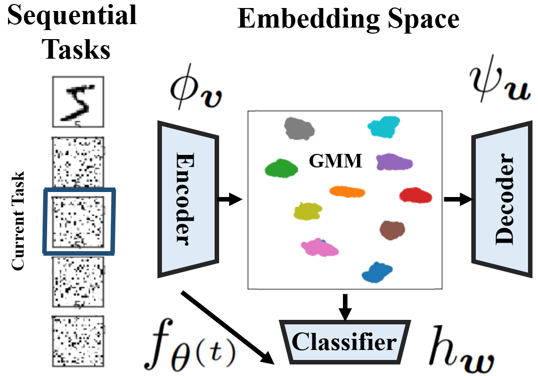
Figure 1: Architecture of the proposed framework.

Let at time $t$, the current task $\mathcal{Z}^{(t)}$ with training dataset $\mathcal{Z}^{(t)}=\langle\bm{X}^{(t)},\bm{Y}^{(t)}\rangle$ arrives. We consider classification tasks where the training data points are drawn i.i.d. in pairs from the joint probability distribution, i.e., $(\bm{x}_{i}^{(t)},\bm{y}_{i}^{(t)})\sim p^{(t)}(\bm{x},\bm{y})$ which has the marginal distribution $q^{(t)}$ over $\bm{x}$. We assume that the lifelong learning agent trains a deep neural network $f_{\theta}:\mathbb{R}^{d}\rightarrow\mathbb{R}^{k}$ with learnable weight parameters $\theta$ to map the data points $\bm{X}^{(t)}=[\bm{x}_{1}^{(t)},\ldots,\bm{x}_{n_{t}}^{(t)}]\in\mathbb{R}^{d\times n_{t}}$ to the corresponding one-hot labels $\bm{Y}^{(t)}=[\bm{y}_{1}^{(t)},\ldots,\bm{y}_{n}^{(t)}]\in\mathbb{R}^{k\times n_{t}}$. Learning a single task in isolation is a standard classical learning problem. The agent can solve for the optimal network weight parameters using standard empirical risk minimization (ERM), $\hat{\theta}^{(t)}=\arg\min_{\theta}\hat{e}_{\theta}=\arg\min_{\theta}\sum_{i}\mathcal{L}_{d}(f_{\theta}(\bm{x}_{i}^{(t)}),\bm{y}_{i}^{(t)})$, where $\mathcal{L}_{d}(\cdot)$ is a proper loss function, e.g., cross entropy. Given large enough number of labeled data points $n_{t}$, the model trained on a single task $\mathcal{Z}^{(t)}$ will generalize well on the task test samples as the empirical risk would be a suitable surrogate for the real risk function (Bayes optimal solution), $e=\mathbb{E}_{(\bm{x},\bm{y})\sim p^{(t)}(\bm{x},\bm{y})}(\mathcal{L}_{d}(f_{\theta^{(t)}}(\bm{x}),\bm{y}))$ Shalev-Shwartz and Ben-David (2014). The agent then can advance to learn the next task, but the challenge is that ERM is unable to tackle catastrophic forgetting as the model parameters are learned using solely the current task data which can potentially have very different distribution. Catastrophic forgetting can be considered as the result of considerable deviations of $\theta^{(T)}$ from past values over $\{\theta^{(t)}\}_{t=1}^{T-1}$ time as a result of drifts in tasks’ distributions $p^{(t)}(\bm{x},\bm{y})$. As a result, the updated $\theta^{(t)}$ can potentially be highly non-optimal for previous tasks. Our idea is to prevent catastrophic forgetting through mapping all tasks’ data into an embedding space, where the tasks share a common distribution. We represent this space by the output space of a deep network mid-layer and we condition updating $\theta^{(t)}$ to what has been learned before in this discriminative embedding space. In other words, we want to train the deep network such the tasks are coupled in the embedding space through updating the parameter $\theta^{(T)}$ conditioned on $\{\theta^{(t)}\}_{t=1}^{T-1}$.

High performance of deep networks stems from learning data-driven and task-dependent high quality features Krizhevsky et al. (2012). In other words, a deep net maps data points into a discriminative embedding space, captured by network layers, where classification can be performed easily, e.g., classes become separable in the embedding. Following this intuition, we consider the deep net $f_{\theta}$ to be combined of of an encoder $\phi_{\bm{v}}(\cdot)$ with learnable parameter $\bm{v}$, i.e., early layers of the network, and a classifier network $h_{\bm{w}}(\cdot)$ with learnable parameters $\bm{w}$, i.e., higher layers of the network. The encoder sub-network $\phi_{\bm{v}}:\mathcal{X}\rightarrow\mathcal{Z}$ maps the data points into the embedding space $\mathcal{Z}\subset\mathbb{R}^{f}$ which describes the input in terms of abstract discriminative features. Note that after training, as a deterministic function, the encoder network changes the input task data distribution.

If the embedding space is discriminative, this distribution can be modeled as a multi-modal distribution for a given task, e.g., Gaussian mixture model (GMM). Catastrophic forgetting occurs because this distribution is not stationery with respect to different tasks. The idea that we want to explore is based on training $\phi_{\bm{v}}$ such that all tasks share a similar distribution in the embedding, i.e., the new tasks are learned such that their distribution in the embedding match the past experience, captured in the shared distribution. Doing so, the embedding space becomes invariant with respect to any learned input task which in turn mitigates catastrophic forgetting.

The key questions is how to adapt the standard supervised learning model $f_{\theta}(\cdot)$ such that the embedding space, captured in the deep network, becomes task-invariant. Following prior discussion, we use experience replay as the main strategy. We expand the base network $f_{\theta}(\cdot)$ into a generative model by amending the model with a decoder $\psi_{\bm{u}}:\mathcal{Z}\rightarrow\mathcal{X}$, with learnable parameters $\bm{u}$. The encoder maps the data representation back to the input space $\mathcal{X}$ and effectively make the pair $(\phi_{\bm{u}},\psi_{\bm{u}})$ an autoencoder. If implemented properly, we would learn a discriminative data distribution in the embedding space which can be approximated by a GMM. This distribution captures our knowledge about past learned tasks. When a new task arrives, pseudo-data points for past tasks can be generated by sampling from this distribution and feeding the samples to the decoder network. These pseudo-data points can be used for experience replay in order to tackle catastrophic forgetting. Additionally, we need to learn the new task such that its distribution matches the past shared distribution. As a result, future pseudo-data points would represent the current task as well. Figure 1 presents a high-level block-diagram visualization of our framework.

4 Optimization Method

Following the above framework, learning the first task ($t=1$) reduces to minimizing discrimination loss term for classification and reconstruction loss for the autoencoder to solve for optimal parameters $\hat{\bm{v}}^{(1)},\hat{\bm{w}^{(1)}}$ and $\hat{\bm{u}^{(1)}}$:

$$\begin{split}\min_{\bm{v},\bm{w},\bm{u}}\sum_{i=1}^{n_{1}}\mathcal{L}_{d}\Big{(}h_{\bm{w}}(\phi_{\bm{v}}\big{(}\bm{x}_{i}^{(1)})\big{)},\bm{y}_{i}^{(1)}\Big{)}+\gamma\mathcal{L}_{r}\Big{(}\psi_{\bm{u}}\big{(}\phi_{\bm{v}}(\bm{x}_{i}^{(1)})\big{)},\bm{x}_{i}^{(1)}\Big{)},\end{split}$$ (1)

where $\mathcal{L}_{r}$ is the reconstruction loss and $\gamma$ is a trade-off parameter between the two loss terms.

Upon learning the first task, as well as subsequent future tasks, we can fit a GMM distribution with $k$ components to the empirical distribution represented by data samples $\{(\phi_{\bm{v}}(\bm{x}_{i}^{(t)}),\bm{y}_{i}^{(t)})_{i=1}^{n_{t}}\}_{t=1}^{T}$ in the embedding space. The intuition behind this possibility is that as the embedding space is discriminative, we expect data points of each class form a cluster in the embedding. Let $\hat{p}_{J}^{(0)}(\bm{z})$ denote this parametric distribution. We update this distribution after learning each task to accumulative what has been learned from the new task to the distribution. As a result, this distribution captures knowledge about past. Upon learning this distribution, experience replay is feasible without saving data points. One can generate pseudo-data points in future through random sampling from $\hat{p}_{J}^{(T-1)}(\bm{z})$ at $t=T$ and then passing the samples through the decoder sub-network. It is also crucial to learn the current task such that its distribution in the embedding matches $\hat{p}_{J}^{(t-1)}(\bm{z})$. Doing so, ensures suitability of GMM to model the empirical distribution. The alternative approach is to use a Variational Auto encoder (VAE), but the discriminator loss helps forming the clusters automatically which in turn makes normal autoencoders a feasible solution.

Let $\mathcal{Z}^{(T)}_{ER}=\langle\bm{X}^{(T)}_{ER},\bm{Y}^{(T)}_{ER}\rangle$ denote the pseudo-dataset, generated at $t=T$. Following our framework, learning subsequent tasks reduces to solving the following problem:

$$\begin{split}&\min_{\bm{v},\bm{w},\bm{u}}\sum_{i=1}^{n_{t}}\mathcal{L}_{d}\Big{(}h_{\bm{w}}\big{(}\phi_{\bm{v}}(\bm{x}_{i}^{(t)})\big{)},\bm{y}_{i}^{(t)}\Big{)}+\gamma\mathcal{L}_{r}\Big{(}\psi_{\bm{u}}\big{(}\phi_{\bm{v}}(\bm{x}_{i}^{(t)})\big{)},\bm{x}_{i}^{(t)}\Big{)}\\ &+\sum_{i=1}^{n_{er}}\mathcal{L}_{d}\Big{(}h_{\bm{w}}\big{(}\phi_{\bm{v}}(\bm{x}_{er,i}^{(T)})\big{)},\bm{y}_{er,i}^{(t)}\Big{)}+\gamma\mathcal{L}_{r}\Big{(}\psi_{\bm{u}}\big{(}\phi_{\bm{v}}(\bm{x}_{er,i}^{(t)})\big{)},\bm{x}_{er,i}^{(t)}\Big{)}\\ &+\lambda\sum_{j=1}^{k}D\Big{(}\phi_{\bm{v}}(q^{(t)}(\bm{X}^{(t)}|C_{j})),\hat{p}_{J}^{(t)}(\bm{Z}_{ER}^{(T)}|C_{j})\Big{)},\end{split}$$ (2)

where $D(\cdot,\cdot)$ is a discrepancy measure, i.e., a metric, between two probability distributions and $\lambda$ is a trade-off parameter. The first four terms in Eq. (2) are empirical classification risk and autoencoder reconstruction loss terms for the current task and the generated pseudo-dataset. The third and the fourth term enforce learning the current task such that the past learned knowledge is not forgotten. The fifth term is added to enforce the learned embedding distribution for the current task to be similar to what has been learned in the past, i.e., task-invariant. Note that we have conditioned the distance between two distribution on classes to avoid class matching challenge, i.e., when wrong classes across two tasks are matched in the embedding, as well as to prevent mode collapse from happening. Class-conditional matching is feasible because we have labels for both distributions. Adding this term guarantees that we can continually use GMM to fit the shared distribution in the embedding space.

The main remaining question is selecting the metric $D(\cdot,\cdot)$ such that it fits our problem. Since we are computing the distance between empirical distributions, through drawn samples, we need a metric that can measure distances between distributions using the drawn samples. Additionally, we must select a metric which has non-vanishing gradients as deep learning optimization techniques are gradient-based methods. For these reasons, common distribution distance measures such as KL divergence and Jensen–Shannon divergence are not suitable Kolouri et al. (2018). We rely on Wasserstein Distance (WD) metric Bonnotte (2013) which has been used extensively in deep learning applications. Since computing WD is computationally expensive, we use Sliced Wasserstein Distance (SWD) Rabin and Peyré (2011) which approximates WD, but can be computed efficiently.

SWD is computed through slicing a high-dimensional distributions. The $d$-dimensional distribution is decomposed into one-dimensional marginal distributions by projecting the distribution into one-dimensional spaces that cover the high-dimensional space. For a given distribution $p$, a one-dimensional slice of the distribution is defined as:

$$\mathcal{R}p(t;\gamma)=\int_{\mathcal{S}}p(\bm{x})\delta(t-\langle\gamma,\bm{x}\rangle)d\bm{x},$$ (3)

where $\delta(\cdot)$ denotes the Kronecker delta function, $\langle\cdot,\cdot\rangle$ denotes the vector dot product, $\mathbb{S}^{d-1}$ is the $d$-dimensional unit sphere and $\gamma$ is the projection direction. In other words, $\mathcal{R}p(\cdot;\gamma)$ is a marginal distribution of $p$ obtained from integrating $p$ over the hyperplanes orthogonal to $\gamma$.

SWD approximates the Wasserstein distance between two distributions $p$ and $q$ by integrating the Wasserstein distances between the resulting sliced marginal distributions of the two distributions over all $\gamma$:

$$SW(p,q)=\int_{\mathbb{S}^{d-1}}W(\mathcal{R}p(\cdot;\gamma),\mathcal{R}q(\cdot;\gamma))d\gamma$$ (4)

where $W(\cdot)$ denotes the Wasserstein distance. The main advantage of using SWD is that it can be computed efficiently as the Wasserstein distance between one-dimensional distributions has a closed form solution and is equal to the $\ell_{p}$-distance between the inverse of their cumulative distribution functions. On the other hand, the $\ell_{p}$-distance between cumulative distribution can be approximated as the $\ell_{p}$-distance between the empirical cumulative distributions which makes SWD suitable in our framework. Finally, to approximate the integral in Eq. (4), we relay on a Monte Carlo style integration and approximate the SWD between $f$-dimensional samples $\{\phi_{\bm{v}}({\mathbf{x}}_{i}^{(t)}\in\mathbb{R}^{f}\sim q^{(t)}\}_{i=1}^{n_{t}}$ and $\{\phi_{\bm{v}}({\mathbf{x}}_{er,i}^{(t)})\in\mathbb{R}^{f}\sim\hat{p}_{J}^{(t)}\}_{j=1}^{n_{t}}$ in the embedding space as the following sum:

$$\begin{split}&SW^{2}(\phi_{\bm{v}}(q^{(t)}),\hat{p}_{J}^{(t)})\approx\\ &\frac{1}{L}\sum_{l=1}^{L}\sum_{i=1}^{n_{t}}|\langle\gamma_{l},\phi_{\bm{v}}({\mathbf{x}}_{t_{l}[i]}^{(t)}\rangle)-\langle\gamma_{l},\phi_{\bm{v}}({\mathbf{x}}_{t_{l}[er,i]}^{(t)})\rangle|^{2}\end{split}$$ (5)

where $\gamma_{l}\in\mathbb{S}^{f-1}$ denote random samples that are drawn from the unit $f$-dimensional ball $\mathbb{S}^{f-1}$, and $s_{l}[i]$ and $t_{l}[i]$ are the sorted indices of $\{\gamma_{l}\cdot\phi_{\bm{v}}({\mathbf{x}}_{i})\}_{i=1}^{n_{t}}$ for the two one-dimensional distributions. We utilize the SWD as the discrepancy measure between the distributions in Eq. (2) to learn each task. We tackle catastrophic forgetting using the proposed procedure. Our algorithm, Continual Learning using Encoded Experience Replay (CLEER) is summarized in Algorithm 1.

Algorithm 1 $\mathrm{CLEER}\left(L,\lambda\right)$

1:Input: data $\mathcal{D}^{(t)}=(\bm{X}^{(t)},\bm{Y}^{(t)})_{t=1}^{T_{\text{Max}}}$.

2:Pre-training: learning the first task ($t=1$)

3:     $\hat{\theta}^{(1)}=(\bm{u}^{(1)},\bm{v}^{(1)},\bm{w}^{(1)})=$$\arg\min_{\theta}\sum_{i}\mathcal{L}_{d}(f_{\theta}(\bm{x}_{i}^{(t)}),\bm{y}_{i}^{(t)})+\gamma\mathcal{L}_{r}(\psi_{\bm{u}}(\phi_{\bm{v}}(\bm{x}_{i}^{(1)})),\bm{x}_{i}^{(1)})$

4:Estimate $\hat{p}_{J}^{(0)}(\cdot)$ using $\{\phi_{\bm{v}}(\bm{x}_{i}^{(1)}))\}_{i=1}^{n_{t}}$

5:for $t=2,\ldots,T_{\text{Max}}$  do

6:    Generate pseudo dataset:

7:         $\mathcal{D}_{\text{ER}}=\{(\bm{x}_{er,i}^{(t)}=\psi(\bm{z}_{er,i}^{(t)}),\bm{y}_{er,i}^{(t)})\sim\hat{p}_{J}^{(t-1)}(\cdot)\}_{i=1}^{n_{er}}$

8:    Update learnable parameters using pseudo dataset:) Eq. (2)

9:    Estimate: $\hat{p}_{J}^{(t)}(\cdot)$

10:         use $\{\phi_{\bm{v}}(\bm{x}_{i}^{(t)})),\phi_{\bm{v}}(\bm{x}_{er,i}^{(t)}))\}_{i=1}^{n_{t}}$

11:end for

5 Theoretical Justification

We use existing theoretical results about using optimal transport within domain adaptation Redko et al. (2017), to justify why our algorithm can tackle catastrophic forgetting. Note that the hypothesis class in our learning problem is the set of all functions represented by the network $f_{\theta}(\cdot)$ parameterized by $\theta$. For a given model in this class, let $e_{t}$ denote the observed risk for a particular task $\mathcal{Z}^{(t)}$ and $e^{J}_{t}$ denote the observed risk for learning the network on samples of the distribution $\hat{p}_{J}^{(t-1)}$. We rely on the following theorem.

Theorem 1 Redko et al. (2017): Consider two tasks $\mathcal{Z}^{(t)}$ and $\mathcal{Z}^{(t^{\prime})}$, and a model $f_{\theta^{(t^{\prime})}}$ trained for $\mathcal{Z}^{(t^{\prime})}$, then for any $d^{\prime}>d$ and $\zeta<\sqrt{2}$, there exists a constant number $N_{0}$ depending on $d^{\prime}$ such that for any $\xi>0$ and $\min(n_{t},n_{t^{\prime}})\geq\max(\xi^{-(d^{\prime}+2),1})$ with probability at least $1-\xi$ for all $f_{\theta^{(t^{\prime})}}$, the following holds:

$$\begin{split}e_{t}\leq&e_{t^{\prime}}+W(\hat{p}^{(t)},\hat{p}^{(t^{\prime})})+e_{\mathcal{C}}(\theta^{*})+\\ &\sqrt{\big{(}2\log(\frac{1}{\xi})/\zeta\big{)}}\big{(}\sqrt{\frac{1}{n_{t}}}+\sqrt{\frac{1}{n_{t^{\prime}}}}\big{)},\end{split}$$ (6)

where $W(\cdot)$ denotes the Wasserstein distance between empirical distributions of the two tasks and $\theta^{*}$ denotes the optimal parameter for training the model on tasks jointly, i.e., $\theta^{*}=\arg\min_{\theta}e_{\mathcal{C}}(\theta)=\arg\min_{\theta}\{e_{t}+e_{t^{\prime}}\}$.

We observe from Theorem 1 that performance, i.e., real risk, of a model learned for task $\mathcal{Z}^{(t^{\prime})}$ on another task $\mathcal{Z}^{(t)}$ is upper-bounded by four terms: i) model performance on task $\mathcal{Z}^{(t^{\prime})}$, ii) the distance between the two distributions, iii) performance of the jointly learned model $f_{\theta^{*}}$, and iv) a constant term which depends on the number of data points for each task. Note that we do not have a notion of time in this Theorem and the roles of $\mathcal{Z}^{(t)}$ and $\mathcal{Z}^{(t^{\prime})}$ can be shuffled and the theorem would still hold. In our framework, we consider the task $\mathcal{Z}^{(t^{\prime})}$, to be the pseudo-task, i.e., the task derived by drawing samples from $\hat{p}_{J}^{t^{\prime}}$ and then feeding the samples to the decoder sub-network. We use this result to conclude the following lemma.

Lemma 1 : Consider CLEER algorithm for lifelong learning after $\mathcal{Z}^{(T)}$ is learned at time $t=T$. Then all tasks $t<T$ and under the conditions of Theorem 1, we can conclude the following inequality:

$$\begin{split}e_{t}\leq&e_{T-1}^{J}+W(\hat{q}^{(t)},\psi(\hat{p}_{J}^{(t)}))+\sum_{s=t}^{T-2}W(\psi(\hat{p}_{J}^{(s)}),\psi(\hat{p}_{J}^{(s+1)}))\\ &+e_{\mathcal{C}}(\theta^{*})+\sqrt{\big{(}2\log(\frac{1}{\xi})/\zeta\big{)}}\big{(}\sqrt{\frac{1}{n_{t}}}+\sqrt{\frac{1}{n_{er,t-1}}}\big{)},\end{split}$$ (7)

Proof: We consider $\mathcal{Z}^{(t)}$ with empirical distribution $\hat{q}^{(t)}$ and the pseudo-task with the distribution $\psi(\hat{p}_{J}^{(T-1)})$ in the network input space, in Theorem 1. Using the triangular inequality on the term $W(\hat{q}^{(t)},\psi(\hat{p}_{J}^{(T-1)}))$ recursively, i.e., $W(\hat{q}^{(t)},\psi(\hat{p}_{J}^{(s)}))\leq W(\hat{p}^{(t)},\psi(\hat{p}_{J}^{(s-1)}))+W(\psi(\hat{p}_{J}^{(s)}),\psi(\hat{p}_{J}^{(s-1)}))$ for all $t\leq s<T$, Lemma 1 can be derived.

Lemma 1 explains why our algorithm can tackle catastrophic forgetting. When future tasks are learned, our algorithms updates the model parameters conditioned on minimizing the upper bound of $e_{t}$ in Eq. 7. Given suitable network structure and in the presence of enough labeled data points, the terms $e_{t-1}^{J}$ and $e_{\mathcal{C}}(\theta^{*})$ are minimized using ERM, and the last constant term would be small. The term $W(\hat{q}^{(t)},\psi(\hat{p}_{J}^{(t)}))$ is minimal because we deliberately fit the distribution $\hat{p}_{J}^{(t)}$ to the distribution $\phi(\hat{q}^{(t)})$ in the embedding space and ideally learn $\phi$ and $\psi$ such that $\psi\approx\phi^{-1}$. This term demonstrates that minimizing the discrimination loss is critical as only then, we can fit a GMM distribution on $\phi(\hat{p}^{(t)})$ with high accuracy. Similarly, the sum terms in Eq 7 are minimized because at $t=s$ we draw samples from $\hat{p}_{J}^{(s-1)}$ and enforce indirectly $\hat{p}_{J}^{(s-1)}\approx\phi(\psi(\hat{p}_{J}^{(s-1)}))$. Since the upper bound of $e_{t}$ in Eq 7 is minimized and conditioned on tightness of the upper bound, the task $\mathcal{Z}^{(t)}$ will not be forgotten.

6 Experimental Validation

We validate our method on learning two sets of sequential tasks: independent permuted MNIST tasks and related digit classification tasks.

6.1 Learning sequential independent tasks

Following the literature, we use permuted MNIST tasks to validate our framework. The sequential tasks involve classification of handwritten images of MNIST ($\mathcal{M}$) dataset LeCun et al. (1990), where pixel values for each data point are shuffled randomly by a fixed permutation order for each task. As a result, the tasks are independent and quite different from each other. Since knowledge transfer across tasks is less likely to happen, these tasks are a suitable benchmark to investigate the effect of an algorithm on mitigating catastrophic forgetting as past learned tasks are not similar to the current task. We compare our method against: a) normal back propagation (BP) as a lower bound, b) full experience replay (FR) of data for all the previous tasks as an upper bound, and c) EWC as a competing weight consolidation framework.

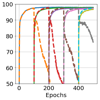
(a) BP vs EWC

(b) CLEER vs FR

Figure 2: Performance results and for permuted MNIST tasks. (Best viewed in color.)

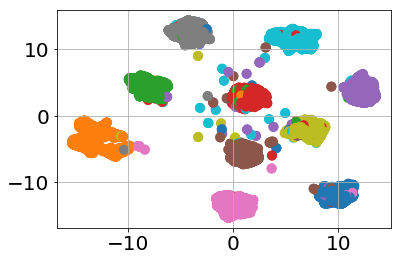
(a) CLEER

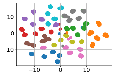
(b) FR

Figure 3: UMAP visualization of CLEER versus FR for MNIST permutation tasks. (Best viewed in color.)

We learn permuted MNIST using a simple multi layer perceptron (MLP) network trained via standard stochastic gradient descent and at each iteration, compute the performance of the network on the testing split of each task data. Figure 2 presents results on five permuted MNIST tasks. Figure 2(a) presents learning curves for BP (dotted curves) and EWC (solid curves) . We observe that EWC is able to address catastrophic forgetting quite well. But a close inspection reveals that as more tasks are learned, the asymptotic performance on subsequent tasks is less than the single task learning performance (roughly $4\%$ less for the fifth task). This can be understood as a side effect of weight consolidation which limits the learning capacity of the network. This in an inherent limitation for techniques that regularize network parameters to prevent catastrophic forgetting. Figure 2(b) presents learning curves for our method (solid curves) versus FR (dotted curves). As expected, FR can prevent catastrophic forgetting perfectly but as we discussed the downside is memory growth challenge. FR result in Figure 2(b) demonstrates that the network learning capacity is sufficient for learning these tasks and if we have a perfect generative model, we can prevent catastrophic forgetting without compromising the network learning capacity. Despite more forgetting in our approach compared to EWC, the asymptotic performance after learning each task, just before advancing to learn the next task, has been improved. We also observe that our algorithm suffers an initial drop in performance of previous tasks, when we proceed to learn a new task. Forgetting beyond this initial forgetting is negligible. This can be understood as the existing distance between $\hat{p}_{J}^{(T-1)}$ and $\phi(q^{(t)})$ at $t=T$. In other words, our method can be improved if more advanced autoencoder structures are used. These results may suggest that catastrophic forgetting may be tackled better if both weight consolidation and experience replay are combined.

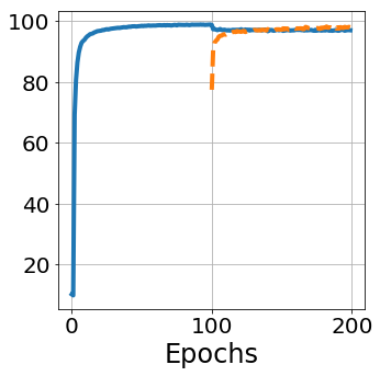
(a) $\mathcal{M}\rightarrow\mathcal{U}$

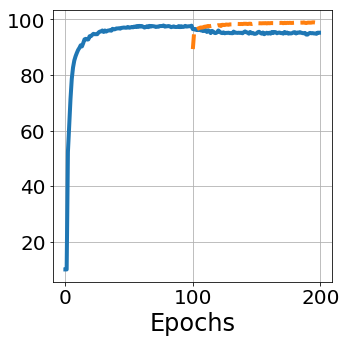
(b) $\mathcal{U}\rightarrow\mathcal{M}$

Figure 4: Performance results on MNIST and USPS digit recognition tasks. (Best viewed in color.)

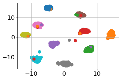
(a) $\mathcal{M}\rightarrow\mathcal{U}$

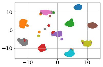
(b) $\mathcal{U}\rightarrow\mathcal{M}$

Figure 5: UMAP visualization for $\mathcal{M}\rightarrow\mathcal{U}$ and $\mathcal{U}\rightarrow\mathcal{M}$ tasks. (Best viewed in color.)

To provide a better intuitive understating, we have also included the representations of the testing data for all tasks in the embedding space of the neural network in Figures  3. We have used UMAP McInnes et al. (2018) to reduce the dimension for visualization purpose. In these figures, each color corresponds to a specific class of digits. We can see that although FR is able to learn all tasks and form distinct clusters for each digit for each task, but five different clusters are formed for each class in the embedding space. This suggests that FR is unable to learn the concept of the same class across different tasks in the embedding space. In comparison, we observe that CLEER is able to match the same class across different tasks, i.e., we have exactly ten clusters for the ten digits. This empirical observation demonstrates that we can model the data distribution in the embedding using a multi-modal distribution such as GMM Heinen et al. (2012).

6.2 Learning sequential tasks in related domains

We performed a second set of experiments on related tasks to investigate the ability of the algorithm to learn new domains. We consider two digit classification datasets for this purpose: MNIST ($\mathcal{M}$) and USPS ($\mathcal{U}$) datasets. Despite being similar, USPS dataset is a more challenging task as the number of training set is smaller, 20,000 compared to 60,000 images. We consider the two possible sequential learning scenarios $\mathcal{M}\rightarrow\mathcal{U}$ and $\mathcal{M}\rightarrow\mathcal{U}$. We resized the USPS images to $28\times 28$ pixels to be able to use the same encoder network for both tasks. The experiments can be considered as a special case of domain adaptation as both tasks are digit recognition tasks but in different domains. To capture relations between the tasks, we use a convolutional network for these experiments.

Figure 4 presents learning curves for these two tasks. We observe that the network retains the knowledge about the first domain, after learning the second domain. We observe that forgetting is negligible compared to unrelated tasks and we have jump-start performance boost. These observations suggests relations between the tasks helps to avoid forgetting. As a result of task similarities, the empirical distribution $\hat{p}_{J}^{(1)}$ can capture the task distribution more accurately. As expected from the theoretical justification, this empirical result suggests the performance of our algorithm depends on closeness of the distribution $\psi(\hat{p}_{J}^{(t)})$ to the distributions of previous tasks and improving probability estimation will increase performance of our approach. We have also presented UMAP visualization of all tasks data in the embedding space in Figures  5. We can see that as expected the distributions are matched in the embedding space.

7 Conclusions

Inspired from CLS theory, we addressed the challenge of catastrophic forgetting for sequential learning of multiple tasks using experience replay. We amend a base learning model with a generative pathway that encodes experience meaningfully as a parametric distribution in an embedding space. This idea makes experience replay feasible without requiring a memory buffer to store task data. The algorithm is able to accumulate knowledge consistently to past learned knowledge as the parametric distribution in the embedding space is enforced to be shared across all tasks. Compared to model-based approaches that regularize the network to consolidate the important weights for past tasks, our approach is able to address catastrophic forgetting without limiting the learning capacity of the network. Future works for our approach may extend to learning new tasks and/or classes with limited labeled data points and investigating how to select the suitable network layer and its dimension as the embedding.

8 Acknowledgment

This material is based upon work supported by the United States Air Force and DARPA under Contract No. FA8750-18-C-0103. Any opinions, findings and conclusions or recommendations expressed in this material are those of the author(s) and do not necessarily reflect the views of the United States Air Force and DARPA.

References

- Aljundi et al. [2018] Rahaf Aljundi, Francesca Babiloni, Mohamed Elhoseiny, Marcus Rohrbach, and Tinne Tuytelaars. Memory aware synapses: Learning what (not) to forget. In Proceedings of the European Conference on Computer Vision (ECCV), pages 139–154, 2018.
- Bonnotte [2013] Nicolas Bonnotte. Unidimensional and evolution methods for optimal transportation. PhD thesis, Paris 11, 2013.
- Chen and Liu [2016] Zhiyuan Chen and Bing Liu. Lifelong machine learning. Synthesis Lectures on Artificial Intelligence and Machine Learning, 10(3):1–145, 2016.
- Diekelmann and Born [2010] S. Diekelmann and J. Born. The memory function of sleep. Nat Rev Neurosci, 11(114), 2010.
- French [1999] Robert M French. Catastrophic forgetting in connectionist networks. Trends in cognitive sciences, 3(4):128–135, 1999.
- Goodfellow et al. [2014] Ian Goodfellow, Jean Pouget-Abadie, Mehdi Mirza, Bing Xu, David Warde-Farley, Sherjil Ozair, Aaron Courville, and Yoshua Bengio. Generative adversarial nets. In Advances in neural information processing systems, pages 2672–2680, 2014.
- Hataya [2018] Ryuichiro Hataya. Ewc pytorch, 2018.
- Heinen et al. [2012] Milton Roberto Heinen, Paulo Martins Engel, and Rafael C Pinto. Using a gaussian mixture neural network for incremental learning and robotics. In The 2012 International Joint Conference on Neural Networks (IJCNN), pages 1–8. IEEE, 2012.
- Isele and Cosgun [2018] David Isele and Akansel Cosgun. Selective experience replay for lifelong learning. In Thirty-Second AAAI Conference on Artificial Intelligence, 2018.
- Kirkpatrick et al. [2017] James Kirkpatrick, Razvan Pascanu, Neil Rabinowitz, Joel Veness, Guillaume Desjardins, Andrei A Rusu, Kieran Milan, John Quan, Tiago Ramalho, Agnieszka Grabska-Barwinska, et al. Overcoming catastrophic forgetting in neural networks. Proceedings of the national academy of sciences, 114(13):3521–3526, 2017.
- Kolouri et al. [2018] Soheil Kolouri, Gustavo K Rohde, and Heiko Hoffmann. Sliced wasserstein distance for learning gaussian mixture models. In Proceedings of the IEEE Conference on Computer Vision and Pattern Recognition, pages 3427–3436, 2018.
- Krizhevsky et al. [2012] Alex Krizhevsky, Ilya Sutskever, and Geoffrey E Hinton. Imagenet classification with deep convolutional neural networks. In Advances in neural information processing systems, pages 1097–1105, 2012.
- Lamprecht and LeDoux [2004] Raphael Lamprecht and Joseph LeDoux. Structural plasticity and memory. Nature Reviews Neuroscience, 5(1):45, 2004.
- LeCun et al. [1990] Yann LeCun, Bernhard E Boser, John S Denker, Donnie Henderson, Richard E Howard, Wayne E Hubbard, and Lawrence D Jackel. Handwritten digit recognition with a back-propagation network. In Advances in neural information processing systems, pages 396–404, 1990.
- McClelland et al. [1995] James L McClelland, Bruce L McNaughton, and Randall C O’reilly. Why there are complementary learning systems in the hippocampus and neocortex: insights from the successes and failures of connectionist models of learning and memory. Psychological review, 102(3):419, 1995.
- McInnes et al. [2018] Leland McInnes, John Healy, and James Melville. Umap: Uniform manifold approximation and projection for dimension reduction. arXiv preprint arXiv:1802.03426, 2018.
- Morgenstern et al. [2014] Yaniv Morgenstern, Mohammad Rostami, and Dale Purves. Properties of artificial networks evolved to contend with natural spectra. Proceedings of the National Academy of Sciences, 111(Supplement 3):10868–10872, 2014.
- Rabin and Peyré [2011] Julien Rabin and Gabriel Peyré. Wasserstein regularization of imaging problem. In 2011 18th IEEE International Conference on Image Processing, pages 1541–1544. IEEE, 2011.
- Rasch and Born [2013] B. Rasch and J. Born. About sleep’s role in memory. Physiol Rev, 93:681–766, 2013.
- Redko et al. [2017] Ievgen Redko, Amaury Habrard, and Marc Sebban. Theoretical analysis of domain adaptation with optimal transport. In Joint European Conference on Machine Learning and Knowledge Discovery in Databases, pages 737–753. Springer, 2017.
- Robins [1995] Anthony Robins. Catastrophic forgetting, rehearsal and pseudorehearsal. Connection Science, 7(2):123–146, 1995.
- Roth et al. [2017] Kevin Roth, Aurelien Lucchi, Sebastian Nowozin, and Thomas Hofmann. Stabilizing training of generative adversarial networks through regularization. In Advances in neural information processing systems, pages 2018–2028, 2017.
- Schaul et al. [2016] Tom Schaul, John Quan, Ioannis Antonoglou, and David Silver. Prioritized experience replay. In IJCLR, 2016.
- Shalev-Shwartz and Ben-David [2014] Shai Shalev-Shwartz and Shai Ben-David. Understanding machine learning: From theory to algorithms. Cambridge university press, 2014.
- Shin et al. [2017] Hanul Shin, Jung Kwon Lee, Jaehong Kim, and Jiwon Kim. Continual learning with deep generative replay. In Advances in Neural Information Processing Systems, pages 2990–2999, 2017.
- Srivastava et al. [2017] Akash Srivastava, Lazar Valkov, Chris Russell, Michael U Gutmann, and Charles Sutton. Veegan: Reducing mode collapse in gans using implicit variational learning. In Advances in Neural Information Processing Systems, pages 3308–3318, 2017.
- Zenke et al. [2017] Friedemann Zenke, Ben Poole, and Surya Ganguli. Continual learning through synaptic intelligence. In Proceedings of the 34th International Conference on Machine Learning-Volume 70, pages 3987–3995. JMLR. org, 2017.