The Dynamical Diquark Model: First Numerical Results

Abstract

We produce the first numerical predictions of the dynamical diquark model of multiquark exotic hadrons. Using Born-Oppenheimer potentials calculated numerically on the lattice, we solve coupled and uncoupled systems of Schrödinger equations to obtain mass eigenvalues for multiplets of states that are, at this stage, degenerate in spin and isospin. Assuming reasonable values for these fine-structure splittings, we obtain a series of bands of exotic states with a common parity eigenvalue that agree well with the experimentally observed charmoniumlike states, and we predict a number of other unobserved states. In particular, the most suitable fit to known pentaquark states predicts states below the charmonium-plus-nucleon threshold. Finally, we examine the strictest form of Born-Oppenheimer decay selection rules for exotics and, finding them to fail badly, we propose a resolution by relaxing the constraint that exotics must occur as heavy-quark spin-symmetry eigenstates.

1 Introduction

The existence of multiquark exotic hadrons is now a well-established feature of strong-interaction physics. At least 35 such states in the heavy quark-antiquark ($Q\!=\!c$ or $b$) sector have been experimentally established at various levels of statistical significance. Many have been observed beyond the $5\sigma$ level at either multiple facilities, or through multiple production or decay channels, or both. A number of reviews in the recent literature Lebed et al. (2017); Chen et al. (2016); Hosaka et al. (2016); Esposito et al. (2016); Guo et al. (2018); Ali et al. (2017); Olsen et al. (2018); Karliner et al. (2018); Yuan (2018) summarize both experimental and theoretical developments.

Yet, even after many years of intensive study, no single theoretical model has emerged to provide a successful, unified picture for understanding the spectroscopy, decay patterns, and structure of these novel states. The most heavily studied alternatives in this regard, including hadronic molecules, diquarks, hadroquarkonium, hybrids, and kinematical threshold effects, both their benefits and drawbacks, are amply discussed in the aforementioned reviews. The complete spectrum might turn out to rely upon a delicate interplay of several of these physical frameworks, meaning that each one must be fully understood before a global model of the exotics can be confidently constructed.

In this work we employ a model in which the exotics are constructed from quasi-bound heavy-light diquarks $\delta^{\vphantom{1}},{\bar{\delta}}$, which are formed via the attractive channels ${\bf 3}\!\otimes\!{\bf 3}\!\to\!\bar{\bf 3}$ [$\delta\!\equiv\!(Qq)_{\bar{\bf 3}}$] and $\bar{\bf 3}\!\otimes\!\bar{\bf 3}\!\to\!{\bf 3}$ [${\bar{\delta}}\!\equiv\!(\bar{Q}{\bar{q}}^{\prime})_{\bf 3}$] between the color-triplet quarks. The most influential early application of diquarks to the problem of heavy exotics Maiani et al. (2005) treats tetraquarks as bound ($\delta^{\vphantom{1}}{\bar{\delta}}$) molecules in a Hamiltonian formalism, using as interaction operators the spin-spin couplings between the various component quarks. A later variant of this approach Maiani et al. (2014) restricted the interactions to spin-spin couplings between quarks within either the $\delta^{\vphantom{1}}$ or the ${\bar{\delta}}$. Reference Anselmino et al. (1993) provides a detailed review of diquark phenomenology prior to the discovery of the heavy exotics.

Such an approach inspired the development of the dynamical diquark picture Brodsky et al. (2014), in which some of the light quarks created in the production process of the ${Q\bar{Q}}$ pair coalesce with these heavy quarks to form a $\delta^{\vphantom{1}}$-${\bar{\delta}}$ pair. Due to the large energies available in either $b\!\to\!c$ or collider processes in which exotics are produced, the $\delta^{\vphantom{1}}$-${\bar{\delta}}$ pair can achieve through recoil a large spatial separation ($>\!1$ fm) before being forced by confinement either to form a single tetraquark state, or if the energy is sufficiently high, for the color flux tube between the $\delta^{\vphantom{1}}$-${\bar{\delta}}$ pair to fragment to create a baryon-antibaryon pair. The key feature of this picture is a mechanism for producing multiquark states that are spatially large yet strongly bound. Indeed, the successive accretion of additional quarks through the color-triplet binding mechanism Brodsky and Lebed (2015) can be used to interpret pentaquark states as triquark-diquark states, ${\bar{\theta}}\delta^{\vphantom{1}}\!\equiv\![\bar{Q}(q_{1}q_{2})_{\bar{\bf 3}}]^{\vphantom{(}}_{\bf 3}(Qq_{3})_{\bar{\bf 3}}$ Lebed (2015). The effectiveness of this mechanism is clearly limited by competition from the attractive $\bar{Q}Q$ and $\bar{Q}q$ channels, and a full theory of multiquark hadrons would allow for including all possible configurations simultaneously. One important step in this much larger project is to uncover the predictions of the $\delta^{\vphantom{1}}$-${\bar{\delta}}$ mechanism and see if the current data provides support for the existence of such states.

The means by which the dynamical diquark picture may be realized as a fully predictive model, including spectroscopy and decay selection rules, is the subject of Ref. Lebed (2017). In the original proposal of the picture Brodsky et al. (2014), the estimated size of the $Z_{c}^{-}(4430)$ resonance appearing in $B^{0}\!\to\!(\psi(2S)\pi^{-})K^{+}$ follows from taking a $\delta^{\vphantom{1}}$-${\bar{\delta}}$ pair (of known masses) produced in the decay to recoil against the $K^{+}$. Since the diquarks, like quarks, are color triplets, a Cornell Coulomb-plus-linear potential Eichten et al. (1978, 1980) was assumed. The final separation of the $\delta^{\vphantom{1}}$-${\bar{\delta}}$ pair upon coming relatively to rest was calculated to be 1.16 fm.

The significance of this classical turning point in forming the exotic state from the $\delta^{\vphantom{1}}$-${\bar{\delta}}$ pair was tied in Refs. Brodsky et al. (2014); Lebed (2017) to the Wentzel-Kramers-Brillouin (WKB) approximation. The WKB transition wave function scales as $1/\sqrt{p}$, where $p$ is the classical relative momentum of the constituents. One therefore expects the color flux tube between the $\delta^{\vphantom{1}}$-${\bar{\delta}}$ pair to stretch nearly to its classical limit. Such a state is spatially large but still exhibits unscreened strong interactions between all of its components. It also possesses two heavy, slow-moving sources ($\delta^{\vphantom{1}}$ and ${\bar{\delta}}$) connected by a lighter (mostly gluonic) field susceptible to more rapid changes. Analogous comments apply to ${\bar{\theta}}$-$\delta^{\vphantom{1}}$ states. These properties indicate that the system can be characterized well by use of the Born-Oppenheimer (BO) approximation Born and Oppenheimer (1927).

Although more familiar from its applications to atomic and molecular systems, the BO approximation has also been implemented in particle physics. In fact, its use as a fundamental tool in lattice-QCD calculations was initiated decades ago Griffiths et al. (1983). The relevant physical observables are the energies of the light degrees of freedom (d.o.f.) that connect a heavy, and hence static, ${Q\bar{Q}}$ pair; such energies as a function of ${Q\bar{Q}}$ separation and orientation are called BO potentials. While multiple aspects of this problem in strong-interaction physics have been studied in the intervening years, the ones most relevant to the present work involve the calculation of the BO potentials and its eigenvalues, which in turn give the masses of heavy-quark hybrid mesons; short overviews of the key lattice papers in this regard appear in Refs. Berwein et al. (2015); Lebed and Swanson (2018). For many years, the most accurate lattice results of hybrid static potentials for substantial ${Q\bar{Q}}$ separation have been those of Juge, Kuti, and Morningstar Juge et al. (1998, 1999, 2003); Mor . Very recently, however, a new collaboration Capitani et al. (2019) has begun to improve upon these results. In addition, high-quality simulations focusing upon small ${Q\bar{Q}}$ separations have been performed Bali and Pineda (2004). Also of note are lattice simulations of two heavy quark-antiquark pairs, which study the crossover between hadron molecule and $\delta^{\vphantom{1}}$-${\bar{\delta}}$ configurations Bicudo et al. (2017).

A prototype of the approach underlying the present work is provided by Ref. Berwein et al. (2015), which supposes the known (neutral) exotics to be hybrid mesons, and then develops an effective field-theory formalism for computing their spectrum, using the BO potentials as input to the Schrödinger equations. The first treatment of multiquark exotic hadrons using the BO formalism appeared in Refs. Braaten (2013); Braaten et al. (2014a, b). In these works, the valence light ${q\bar{q}}$ pair (for tetraquarks) is treated as belonging to the light d.o.f. In contrast, the light quarks in the dynamical diquark model belong to the diquarks, which in turn are treated as the heavy, pointlike sources, while the light d.o.f. are purely gluonic (or include sea quarks).

This paper carries out one of the central proposals of Ref. Lebed (2017): a numerical calculation of the spectrum of $\delta^{\vphantom{1}}$-${\bar{\delta}}$ and ${\bar{\theta}}$-$\delta^{\vphantom{1}}$ hidden-charm states, under the assumption that their basic structure—at least in the last moments of their evolution prior to decay—consists of heavy, slow-moving compact diquarks interacting through the same hybrid BO potentials as those appearing in the ${Q\bar{Q}}$ sector. We solve the resulting Schrödinger equations numerically and identify known exotic states with the eigenstates of the lowest-lying BO potentials. One can already identify a number of assumptions implicit in this strategy; these and several others of equal significance are discussed below. Nevertheless, the initial results are quite encouraging: Choosing to fix to either $X(3872)$ or $Z_{c}(4430)$ as a reference $\delta^{\vphantom{1}}$-${\bar{\delta}}$ state, one obtains a spectrum broadly consistent with the pattern of the known tetraquark states, and for which the excited states above the ground-state band [$\Sigma^{+}_{g}(1S)$] naturally have substantial spatial extent. In the pentaquark case, fixing to, e.g., $P_{c}(4312)$ and $P_{c}(4457)$ predicts the masses of numerous unseen states.

In carrying out calculations in this scheme, one must keep in mind the central difficulty with diquark models (as discussed in any of the reviews Lebed et al. (2017); Chen et al. (2016); Hosaka et al. (2016); Esposito et al. (2016); Guo et al. (2018); Ali et al. (2017); Olsen et al. (2018); Karliner et al. (2018); Yuan (2018)): the proliferation of many more potential multiquark states than have been observed to date. For example, the $J^{PC}\!=\!1^{++}$ $X(3872)$ appears to lack an isospin partner Aubert and et al. (2005) that would arise from replacing its $u\!\to\!d$ quarks. On the other hand, the isotriplet $1^{+-}$ $Z_{c}(3900)$ lies so close in mass to $X(3872)$ as to suggest some sort of multiplet structure. A truly complete diquark model must explain both the absence of the former and the presence of the latter. While we indicate how the details of this fine structure might be resolved in Sec. 5, for the present work we seek only to establish the broader pattern of multiplets, in particular, as collections of states sorted in mass by their parity eigenvalue.

The organization of this paper is as follows: In Sec. 2 we reprise the notation for dynamical diquark-model states developed in Ref. Lebed (2017); the reader unfamiliar with BO notation appropriate to the “diatomic” system is referred to Appendix A. Section 3 discusses the relevant Schrödinger equations, both uncoupled and coupled versions, as introduced in Ref. Berwein et al. (2015). Details of our numerical approach to solving these equations appear in Appendix B. In Sec. 4 we present our results, and outline the approximations used to obtain them in Sec. 5, describing how these simplifications can be lifted one by one. Finally, Sec. 6 presents our conclusions and directions for subsequent development of the model.

2 Spectrum of the Dynamical Diquark Model

2.1 Tetraquarks

The notation adopted in Ref. Lebed (2017) for states in the dynamical diquark model begins with the notation introduced in Ref. Maiani et al. (2014) for diquark-antidiquark ($\delta^{\vphantom{1}}$-${\bar{\delta}}$) states of good total $J^{PC}$ with zero orbital angular momentum:

$$J^{PC}=0^{++}: X_{0}\equiv\left|0_{\delta}^{\vphantom{1}},0_{\bar{\delta}}\right>_{0}\,,\ \ X_{0}^{\prime}\equiv\left|1_{\delta}^{\vphantom{1}},1_{\bar{\delta}}\right>_{0}\,,$$

$$J^{PC}=1^{++}: X_{1}\equiv\frac{1}{\sqrt{2}}\left(\left|1_{\delta}^{\vphantom{1}},0_{\bar{\delta}}\right>_{1}\!+\left|0_{\delta}^{\vphantom{1}},1_{\bar{\delta}}\right>_{1}\right)\,,$$

$$J^{PC}=1^{+-}: \ \,Z\equiv\frac{1}{\sqrt{2}}\left(\left|1_{\delta}^{\vphantom{1}},0_{\bar{\delta}}\right>_{1}\!-\left|0_{\delta}^{\vphantom{1}},1_{\bar{\delta}}\right>_{1}\right)\,,$$

$$\;Z^{\prime}\equiv\left|1_{\delta}^{\vphantom{1}},1_{\bar{\delta}}\right>_{1}\,,$$

$$J^{PC}=2^{++}: X_{2}\equiv\left|1_{\delta}^{\vphantom{1}},1_{\bar{\delta}}\right>_{2}\,.$$ (1)

The number before each $\delta^{\vphantom{1}}$(${\bar{\delta}}$) subscript is the diquark (antidiquark) spin, and the outer subscript on each ket is the total quark spin $J$. By straightforward use of $9j$ symbols, these states can also be expressed in terms of states of good heavy-quark (${Q\bar{Q}}$) and light-quark (${q\bar{q}}$) spins [from which eigenvalues of the charge-conjugation parity $C$ given in Eq. (1) are immediately determined]. The states in Eq. (1) represent the tetraquark analogues to heavy $S$-wave quark-model states such as $\eta_{Q}$ and $\psi\;(\Upsilon)$.

One then allows for nonzero relative orbital angular momentum $L$ between the $\delta^{\vphantom{1}}$-${\bar{\delta}}$ pair. Using the generic symbol $Y$ for $X_{0},X_{1},Z,Z^{\prime},X_{2}$ in Eq. (1), and ${\bf J}\!=\!{\bf L}\!+\!{\bf S}$, where now $S$ is the total quark spin, one obtains the states $Y^{(J)}_{L}$. In terms of $C_{Y}$, the $C$-parity of the underlying $S$-wave state $Y$, these states have $P\!=\!(-1)^{L}$ and $C\!=\!(-1)^{L}C_{Y}$. Such states include the analogues of the $P$-wave quark-model states $\chi_{Q}$, $h_{Q}$, as well as the $D$-wave, $F$-wave, etc. states. All of these states also possess radial excitations, labeled by the quantum number $n$.

Lastly, one appends the quantum numbers from the Born-Oppenheimer (BO) excitation of the gluon field with respect to the quark state. Given the BO potential with quantum numbers $\Gamma\!\equiv\!\Lambda^{\epsilon}_{\eta}$ as defined in Appendix A, states receive multiplicative factors to their $P$ and $C$ quantum numbers of $\rho\!\equiv\!\epsilon(-1)^{\Lambda}$ and $\kappa\!\equiv\!\eta\epsilon(-1)^{\Lambda}\!=\!\eta\rho$, respectively. In total, and suppressing the radial quantum number $n$, the physical tetraquark eigenstates may be labeled $Y^{(J)\rho\kappa}_{L}$, where

$$P=\rho\,(-1)^{L}\,,\ \ C=\kappa\,(-1)^{L}C_{Y}\,.$$ (2)

The resulting states associated with the lowest BO potentials (as calculated on the lattice) are listed in Table 1. If the light d.o.f. carry nonzero isospin $I$ [e.g., $(cu)(\bar{c}\bar{d})$], then the $C$-parity eigenvalue of the state is replaced by the $G$-parity eigenvalue, $G\!\equiv\!C(-1)^{I}$, where the $C$ eigenvalue is that of the neutral member of the isospin multiplet.

Table 1: Quantum numbers of the lowest tetraquark states expected in the dynamical diquark picture. For each of the expected lowest Born-Oppenheimer potentials, the full multiplet for given $nL$ eigenvalues is presented, using both the state notation developed in Ref. Lebed (2017) and the corresponding $J^{PC}$ eigenvalues. States with $J^{PC}$ not allowed for conventional ${q\bar{q}}$ mesons are indicated in boldface.

BO states	State notation
	State $J^{PC}$
$\Sigma^{+}_{g}(1S)$	$X_{0\,S}^{(0)++}$	$Z_{S}^{(1)++}$, $Z_{S}^{\prime\,(1)++}$	$X_{0\,S}^{\prime\,(0)++}$, $X_{1\,S}^{(1)++}$, $X_{2\,S}^{(2)++}$
	$0^{++}$	$2\times 1^{+-}$	$[0,1,2]^{++}$
$\Sigma^{+}_{g}(1P)$	$X_{0\,P}^{(1)++}$	$[Z_{P}^{(0),\bm{(1)},(2)}]^{++}$, $[Z_{P}^{\prime\,(0),\bm{(1)},(2)}]^{++}$	$X_{0\,P}^{\prime\,(1)++}$,  $[X_{1\,P}^{\bm{(0)},(1),(2)}]^{++}$,  $[X_{2\,P}^{(1),(2),(3)}]^{++}$
	$1^{--}$	$2\times(0,\bm{1},2)^{-+}$	$[1,\ (\bm{0},1,2),\ (1,2,3)]^{--}$
$\Sigma^{+}_{g}(1D)$	$X_{0\,D}^{(2)++}$	$[Z_{D}^{(1),\bm{(2)},(3)}]^{++}$, $[Z_{D}^{\prime\,(1),\bm{(2)},(3)}]^{++}$	$X_{0\,D}^{\prime\,(2)++}$,  $[X_{1\,D}^{(1),(2),(3)}]^{++}$,  $[X_{2\,D}^{(0),(1),(2),(3),(4)}]^{++}$
	$2^{++}$	$2\times(1,\bm{2},3)^{+-}$	$[2,\ (1,2,3),\ (0,1,2,3,4)]^{++}$
$\Pi^{+}_{u}(1P)$ &	$X_{0\,P}^{(1)-+}$	$[Z_{P}^{(0),(1),(2)}]^{-+}$, $[Z_{P}^{\prime\,(0),(1),(2)}]^{-+}$	$X_{0\,P}^{\prime\,(1)-+}$,  $[X_{1\,P}^{\bm{(0)},(1),\bm{(2)}}]^{-+}$,  $[X_{2\,P}^{(1),\bm{(2)},(3)}]^{-+}$
$\Sigma^{-}_{u}(1P)$	$1^{+-}$	$2\times(0,1,2)^{++}$	$[1,\ (\bm{0},1,\bm{2}),\ (1,\bm{2},3)]^{+-}$
$\Pi^{-}_{u}(1P)$	$X_{0\,P}^{\bm{(1)}+-}$	$[Z_{P}^{\bm{(0)},(1),(2)}]^{+-}$, $[Z_{P}^{\prime\,\bm{(0)},(1),(2)}]^{+-}$	$X_{0\,P}^{\prime\,\bm{(1)}+-}$,  $[X_{1\,P}^{(0),\bm{(1)},(2)}]^{+-}$,  $[X_{2\,P}^{\bm{(1)},(2),\bm{(3)}}]^{+-}$
	$\bm{1}^{-+}$	$2\times(\bm{0},1,2)^{--}$	$[\bm{1},\ (0,\bm{1},2),\ (\bm{1},2,\bm{3})]^{-+}$
$\Sigma^{-}_{u}(1S)$	$X_{0\,S}^{(0)-+}$	$Z_{S}^{(1)-+}$, $Z_{S}^{\prime\,(1)-+}$	$X_{0\,S}^{\prime\,(0)-+}$, $X_{1\,S}^{\bm{(1)}-+}$, $X_{2\,S}^{(2)-+}$
	$0^{-+}$	$2\times 1^{--}$	$[0,\bm{1},2]^{-+}$
$\Pi^{+}_{u}(1D)$ &	$X_{0\,D}^{(2)-+}$	$[Z_{D}^{(1),(2),(3)}]^{-+}$, $[Z_{D}^{\prime\,(1),(2),(3)}]^{-+}$	$X_{0\,D}^{\prime\,(2)-+}$,  $[X_{1\,D}^{\bm{(1)},(2),\bm{(3)}}]^{-+}$,  $[X_{2\,D}^{(0),\bm{(1)},(2),\bm{(3)},(4)}]^{-+}$
$\Sigma^{-}_{u}(1D)$	$2^{-+}$	$2\times(1,2,3)^{--}$	$[2,\ (\bm{1},2,\bm{3}),\ (0,\bm{1},2,\bm{3},4)]^{-+}$

2.2 Pentaquarks

Much of the same construction holds for the ${\bar{\theta}}$-$\delta^{\vphantom{1}}$ pentaquarks. In that case, the states analogous to those in Eq. (1) are denoted by Lebed (2017):

$$J^{P}={\frac{1}{2}}^{-}\!\!:\ P_{\frac{1}{2}}\equiv\left|{\displaystyle{\frac{1}{2}}}_{\bar{\theta}},0_{\delta}^{\vphantom{1}}\right>_{\frac{1}{2}},\ \ P^{\prime}_{\frac{1}{2}}\equiv\left|{\displaystyle{\frac{1}{2}}}_{\bar{\theta}},1_{\delta}^{\vphantom{1}}\right>_{\frac{1}{2}},$$

$$J^{P}={\frac{3}{2}}^{-}\!\!:\ P_{\frac{3}{2}}\equiv\left|{\displaystyle{\frac{1}{2}}}_{\bar{\theta}},1_{\delta}^{\vphantom{1}}\right>_{\frac{3}{2}}.$$ (3)

The number before each ${\bar{\theta}}$($\delta^{\vphantom{1}}$) subscript is the triquark (diquark) spin, and the outer subscript on each ket is the total quark spin $J$. In this list, the light diquark internal to ${\bar{\theta}}$ is restricted to carry spin 0 (as well $ud$ flavor content with isospin 0), since all the known heavy pentaquark candidates Aaij and et al. (2019), $P_{c}(4312)$, $P_{c}(4380)$, $P_{c}(4440)$, and $P_{c}(4457)$, appear in the decay of $\Lambda_{b}$, whose light $ud$ valence quarks carry these attributes. In general, 6 additional states, for which the light diquark in ${\bar{\theta}}$ carries spin 1, can be defined.

The relative orbital angular momentum $L$ and the BO potential quantum numbers $\Gamma\!\equiv\!\Lambda^{\epsilon}$ are then incorporated. Since the ${\bar{\theta}}$ and $\delta^{\vphantom{1}}$ components cannot form a charge-conjugate pair, the core states of Eq. (3) are not $C$ eigenstates, and the BO potentials $\Lambda^{\epsilon}$ are not $\eta$ eigenstates (see Appendix A). Defining $\rho\!\equiv\!\epsilon(-1)^{\Lambda}$ as before, one obtains

$$P=\rho\,(-1)^{L+1}\,.$$ (4)

Suppressing the radial quantum number $n$, the physical pentaquark eigenstates may be labeled $P^{(J)\rho}_{SL}$, where $S$ now denotes the total quark spin. The resulting states associated with the lowest BO potentials (as calculated on the lattice) are listed in Table 2.

Table 2: Quantum numbers of the lowest pentaquark states expected in the dynamical triquark-diquark picture. For each of the expected lowest Born-Oppenheimer potentials, the full multiplet for given $nL$ eigenvalues is presented, using both the state notation developed in Ref. Lebed (2017) and the corresponding $J^{P}$ eigenvalues.

BO states	State notation
	State $J^{P}$
$\Sigma^{+}(1S)$	$P_{\frac{1}{2}\,S}^{(\frac{1}{2})+}$, $P_{\frac{1}{2}\,S}^{\prime\,(\frac{1}{2})+}$	$P_{\frac{3}{2}\,S}^{(\frac{3}{2})+}$
	$2\times{\frac{1}{2}}^{-}_{\vphantom{\dagger}}$	${\frac{3}{2}}^{-}$
$\Sigma^{+}(1P)$	$\Big{[}P_{\frac{1}{2}\,P}^{(\frac{1}{2}),(\frac{3}{2})}\Big{]}^{+},\ \Big{[}P_{\frac{1}{2}\,P}^{\prime\,(\frac{1}{2}),(\frac{3}{2})}\Big{]}^{+}$	$\Big{[}P_{\frac{3}{2}\,P}^{(\frac{1}{2}),(\frac{3}{2}),(\frac{5}{2})}\Big{]}^{+}$
	$2\times\left(\frac{1}{2},\frac{3}{2}\right)^{+}_{\vphantom{\dagger}}$	$\left(\frac{1}{2},\frac{3}{2},\frac{5}{2}\right)^{+}$
$\Sigma^{+}(1D)$	$\Big{[}P_{\frac{1}{2}\,D}^{(\frac{3}{2}),(\frac{5}{2})}\Big{]}^{+},\ \Big{[}P_{\frac{1}{2}\,D}^{\prime\,(\frac{3}{2}),(\frac{5}{2})}\Big{]}^{+}$	$\Big{[}P_{\frac{3}{2}\,D}^{(\frac{1}{2}),(\frac{3}{2}),(\frac{5}{2}),(\frac{7}{2})}\Big{]}^{+}$
	$2\times\left(\frac{3}{2},\frac{5}{2}\right)^{-}_{\vphantom{\dagger}}$	$\left(\frac{1}{2},\frac{3}{2},\frac{5}{2},\frac{7}{2}\right)^{-}$
$\Pi^{+}(1P)$ &	$\Big{[}P_{\frac{1}{2}\,P}^{(\frac{1}{2}),(\frac{3}{2})}\Big{]}^{-},\ \Big{[}P_{\frac{1}{2}\,P}^{\prime\,(\frac{1}{2}),(\frac{3}{2})}\Big{]}^{-}$	$\Big{[}P_{\frac{3}{2}\,P}^{(\frac{1}{2}),(\frac{3}{2}),(\frac{5}{2})}\Big{]}^{-}$
$\Sigma^{-}(1P)$	$2\times\left(\frac{1}{2},\frac{3}{2}\right)^{-}_{\vphantom{\dagger}}$	$\left(\frac{1}{2},\frac{3}{2},\frac{5}{2}\right)^{-}$
$\Pi^{-}(1P)$	Same as $\Sigma^{+}(1P)_{\vphantom{\big{[}}}$
$\Sigma^{-}(1S)$	$P_{\frac{1}{2}\,S}^{(\frac{1}{2})-}$, $P_{\frac{1}{2}\,S}^{\prime\,(\frac{1}{2})-}$	$P_{\frac{3}{2}\,S}^{(\frac{3}{2})-}$
	$2\times{\frac{1}{2}}^{+}_{\vphantom{\dagger}}$	${\frac{3}{2}}^{+}$
$\Pi^{+}(1D)$ &	$\Big{[}P_{\frac{1}{2}\,D}^{(\frac{3}{2}),(\frac{5}{2})}\Big{]}^{-},\ \Big{[}P_{\frac{1}{2}\,D}^{\prime\,(\frac{3}{2}),(\frac{5}{2})}\Big{]}^{-}$	$\Big{[}P_{\frac{3}{2}\,D}^{(\frac{1}{2}),(\frac{3}{2}),(\frac{5}{2}),(\frac{7}{2})}\Big{]}^{-}$
$\Sigma^{-}(1D)$	$2\times\left(\frac{3}{2},\frac{5}{2}\right)^{+}_{\vphantom{\dagger}}$	$\left(\frac{1}{2},\frac{3}{2},\frac{5}{2},\frac{7}{2}\right)^{+}$

3 Schrödinger Equations for the Born-Oppenheimer Potentials

At its core, the calculation of the spectrum of hybrids in Ref. Berwein et al. (2015) amounts to the use of the BO potentials calculated on the lattice in Refs. Juge et al. (2003); Bali and Pineda (2004) to find the energy eigenvalues of Schrödinger equations between a static ${Q\bar{Q}}$ pair ($c\bar{c}$, $c\bar{b}$, and $b\bar{b}$ are all considered). The relevant Schrödinger equations actually arise directly from QCD through a systematic $1/m_{Q}$ expansion by the application of effective field theories: first NRQCD Caswell and Lepage (1986); Bodwin et al. (1995) (in which the hard scale $m_{Q}$ is integrated out), and then pNRQCD Pineda and Soto (1998); Brambilla et al. (2000) (in which the softer scale of momentum transfer between the ${Q\bar{Q}}$ pair is integrated out). The gluonic pNRQCD static energies between the ${Q\bar{Q}}$ pair are then none other than the BO potentials, which are obtained numerically on the lattice.

Since the fundamental quark mass $m_{Q}$ appears directly in the analysis of Ref. Berwein et al. (2015), the authors take care to identify the details of their renormalization scheme for both $m_{Q}$ and the perturbative short-distance behavior of the potential between the fundamental ${Q\bar{Q}}$ pair. In our case, the corresponding mass $m_{\delta}^{\vphantom{1}}$ is that of the diquark (or $m_{\bar{\theta}}$ for the triquark), which is of course not a fundamental Lagrangian parameter, and therefore in this analysis $m_{\delta}^{\vphantom{1}}$, $m_{\bar{\theta}}$, and the $\delta^{\vphantom{1}}$-${\bar{\delta}}$ and ${\bar{\theta}}$-$\delta^{\vphantom{1}}$ potentials are treated purely phenomenologically.

More central to the current calculation is that the full Schrödinger equations for the “diatomic” system contain not one, but two special points, corresponding to the two heavy-constituent positions, separated by a distance $r$. One expects additional symmetries between the static energies to arise in the limit $r\!\to\!0$, where the cylindrical $D_{\infty h}$ symmetry for the “homonuclear” $\delta^{\vphantom{1}}$-${\bar{\delta}}$ case or the conical $C_{\infty v}$ symmetry for the “heteronuclear” ${\bar{\theta}}$-$\delta^{\vphantom{1}}$ case (see Appendix A and Fig. 1) is supplanted by the higher spherical $O(3)$ symmetry. These $r\!\to\!0$ static energy configurations, transforming as color adjoints in the light d.o.f. and corresponding to degenerate BO potentials in the limit $r\!\to\!0$, are called gluelumps. One finds, for instance, that the $\delta^{\vphantom{1}}$-${\bar{\delta}}$ $\Sigma^{-}_{u}$ and $\Pi^{+}_{u}$ BO potentials approach a single gluelump with $J^{PC}\!=\!1^{+-}$. Additionally, the loss of the single (spherical) symmetry center for $r\!>\!0$ means that the angular part of the Laplacian in the Schrödinger equation is no longer solved by familiar spherical harmonics, but by slightly more complicated forms Landau and Lifshitz (1977).

All $\delta^{\vphantom{1}}$-${\bar{\delta}}$ BO potentials arising from a particular gluelump appear together in a coupled system of Schrödinger equations. The ground-state BO potential $\Sigma^{+}_{g}$ does not mix with others, and therefore appears in an uncoupled equation. While the degenerate BO potentials $\Pi^{+}_{u}$ and $\Pi^{-}_{u}$ carry opposite $\epsilon$ parities, only $\Pi^{+}_{u}(nL)$ produces states with the same $J^{PC}$ quantum numbers as $\Sigma^{-}_{u}(nL)$ for $L\!>\!0$ [$\Pi^{+}_{u}(nS)$ is forbidden by Eq. (19)]. Indeed, $\Pi^{+}_{u}$ is found in lattice simulations to approach $\Sigma^{-}_{u}$ as $r\!\to\!0$, to form the $1^{+-}$ gluelump Brambilla et al. (2000). The Schrödinger equations for $\Pi^{+}_{u}(nL)$ and $\Sigma^{-}_{u}(nL)$ with $L\!>\!0$ therefore must be solved as a coupled system, while those for $\Sigma^{+}_{g}(nL)$, $\Pi^{-}_{u}(nL)$ (with $L\!>\!0$), or $\Sigma^{-}_{u}(nS)$ remain uncoupled. One finds different mass eigenvalues emerging from $\Pi^{\pm}_{u}(1P)$, a lifting of the parity symmetry called $\Lambda$-$\it{doubling}$ Landau and Lifshitz (1977). Higher-mass gluelumps have been found to split into even more BO potentials Brambilla et al. (2000). For example, the $2^{--}$ gluelump supports the BO potentials $\Sigma^{-}_{g}$, $\Pi^{+\prime}_{g}$, and $\Delta^{-}_{g}$; its Schrödinger equations for $D$-wave solutions would couple all three of them. Analogous comments apply to the ${\bar{\theta}}$-$\delta^{\vphantom{1}}$ BO potentials, once the $\eta\!=\!g,u$ subscript is removed.

The radial Schrödinger equations for the uncoupled BO potentials $V_{\Gamma}$ assume the conventional form (with $\hbar\!=\!1$):

$$\left[-\frac{1}{2\mu r^{2}}\partial_{r}r^{2}\partial_{r}\!+\frac{\ell(\ell+1)}{2\mu r^{2}}+V_{\Gamma}(r)\right]\!\psi_{\Gamma}^{(n)}(r)=E_{n}\psi_{\Gamma}^{(n)}(r)\,,$$ (5)

and for the coupled potentials $\Pi^{+}_{u},\Sigma^{-}_{u}$, they read:

$$\left[-\frac{1}{2\mu r^{2}}\partial_{r}r^{2}\partial_{r}\!+\frac{1}{2\mu r^{2}}\left(\begin{array}[]{cc}\ell(\ell+1)+2&2\sqrt{\ell(\ell+1)}\\ 2\sqrt{\ell(\ell+1)}&\ell(\ell+1)\end{array}\right)\right.$$ (15)

$$+\left.\left(\begin{array}[]{cc}V^{\vphantom{\dagger}}_{\Sigma^{-}_{u}}(r)&0\\ 0&V^{\vphantom{\dagger}}_{\Pi^{+}_{u}}(r)\end{array}\right)\right]\!\left(\begin{array}[]{c}\psi^{(n)}_{\Sigma^{-}_{u}}(r)\\ \psi^{(n)^{\vphantom{\dagger}}}_{\Pi^{+}_{u}}(r)\end{array}\right)\!=E_{n}\!\left(\begin{array}[]{c}\psi^{(n)}_{\Sigma^{-}_{u}}(r)\\ \psi^{(n)^{\vphantom{\dagger}}}_{\Pi^{+}_{u}}(r)\end{array}\right).$$

The details of the numerical methods for solving these coupled Schrödinger equations, using the state-of-the-art techniques of Refs. Johnson (1978) and Hutson (1994), are discussed in Appendix B.

4 Results

Using the techniques of Sec. 3, one predicts the full spectrum of states in the dynamical diquark model with only two further inputs: the diquark masses $m_{\delta}^{\vphantom{1}}$ and $m_{\bar{\delta}}$ (or triquark mass $m_{\bar{\theta}}$) and specific functional forms $V(r)$ for the BO potentials $\Gamma$. The potentials are intrinsically nonperturbative in nature and can only be computed from first principles by using lattice QCD simulations. In this regard we apply the results of Refs. Juge et al. (1998, 1999, 2003); Mor , especially the online summary of results in Ref. Mor , to which we refer as JKM; and separately, we apply the results of the very recent calculations of Ref. Capitani et al. (2019), to which we refer as CPRRW. Furthermore, since the corresponding calculation for the ground-state ($\Sigma_{g}^{+}$) BO potential for the $c\bar{c}$ system with both component masses given by $m_{c}$ would generate the conventional charmonium spectrum, we also include for $\Sigma_{g}^{+}$ cases the phenomenological Cornell potential used in the fit of Ref. Barnes et al. (2005) (but suppressing spin-dependent couplings), to which we refer as BGS.

The numerical results are summarized in Tables 3, 4, and 5 for hidden-charm tetraquarks and Table 7 for hidden-charm pentaquarks. We take $m_{\bar{\delta}}\!=\!m_{\delta}^{\vphantom{1}}$ in each case. Fine-structure spin-dependent mass splittings among the states of each level $\Gamma(nL)$ (as enumerated in Tables 1 and 2) are neglected in the present calculation, and the approach to include them in future calculations is discussed in detail in Sec. 5.

Table 3: Mass eigenvalues $M$ (in GeV) for hidden-charm dynamical diquark states that are eigenstates of the indicated BO potentials corresponding to quantum numbers $nL$, for given diquark masses $m_{\delta}$ (in GeV). The particular form of the BO potential used is that given by lattice simulations JKM Mor or CPRRW Capitani et al. (2019), or (for the $\Sigma^{+}_{g}$ potential) by the Cornell potential obtained from a fit BGS Barnes et al. (2005) to conventional charmonium. Also predicted are the corresponding expectation values for the length scales ${\langle 1/r\rangle}^{-1}$ and $\langle r\rangle$ (in fm). Fixing to the experimental mass of $X(3872)$ or $Z_{c}^{-}(4430)$ predicts $m_{\delta}$ and the whole spectrum, either under the assumption that $X(3872)$ is a $\Sigma^{+}_{g}(1S)$ state or that $Z_{c}(4430)$ is a $\Sigma^{+}_{g}(2S)$ state (as indicated by boldface).

		$X(3872)$				$Z_{c}(4430)$
BO states	Potential	$M$	$m_{\delta}$	${\langle}{1/r}{\rangle}^{-1}$	${\langle}{r}{\rangle}$	$M$	$m_{\delta}$	${\langle}{1/r}{\rangle}^{-1}$	${\langle}{r}{\rangle}$
$\Sigma_{g}^{+}(1S)$	JKM	$\mathbf{3.8711}$	$1.8747$	$0.27202$	$0.36485$	$3.9077$	$1.8946$	$0.27075$	$0.36322$
	CPRRW	$\mathbf{3.8721}$	$1.8535$	$0.27519$	$0.36904$	$3.9108$	$1.8745$	$0.27384$	$0.36694$
	BGS	$\mathbf{3.8718}$	$1.9402$	$0.21347$	$0.30268$	$3.8824$	$1.9462$	$0.21301$	$0.30221$
$\Sigma_{g}^{+}(2S)$	JKM	$4.4430$	$1.8747$	$0.42698$	$0.69081$	$\mathbf{4.4782}$	$1.8946$	$0.42524$	$0.68825$
	CPRRW	$4.4410$	$1.8535$	$0.43057$	$0.69640$	$\mathbf{4.4781}$	$1.8745$	$0.42877$	$0.69360$
	BGS	$4.4674$	$1.9402$	$0.42621$	$0.69756$	$\mathbf{4.4781}$	$1.9462$	$0.42562$	$0.69640$
$\Sigma_{g}^{+}(1P)$	JKM	$4.2457$	$1.8747$	$0.48968$	$0.56601$	$4.2816$	$1.8946$	$0.48773$	$0.56392$
	CPRRW	$4.2435$	$1.8535$	$0.49379$	$0.57067$	$4.2814$	$1.8745$	$0.49170$	$0.56834$
	BGS	$4.3471$	$1.9402$	$0.48361$	$0.56787$	$4.3580$	$1.9462$	$0.48285$	$0.56718$
$\Sigma_{g}^{+}(2P)$	JKM	$4.7128$	$1.8747$	$0.62445$	$0.84285$	$4.7473$	$1.8946$	$0.62201$	$0.83982$
	CPRRW	$4.7092$	$1.8535$	$0.62911$	$0.84913$	$4.7456$	$1.8745$	$0.62664$	$0.84564$
	BGS	$4.7416$	$1.9402$	$0.65333$	$0.89663$	$4.7523$	$1.9462$	$0.65243$	$0.89547$
$\Sigma_{g}^{+}(1D)$	JKM	$4.5318$	$1.8747$	$0.66414$	$0.73132$	$4.5669$	$1.8946$	$0.66168$	$0.72853$
	CPRRW	$4.5282$	$1.8535$	$0.66921$	$0.73668$	$4.5653$	$1.8745$	$0.66651$	$0.73365$
	BGS	$4.6151$	$1.9402$	$0.69780$	$0.77323$	$4.6259$	$1.9462$	$0.69690$	$0.77230$
$\Sigma_{g}^{+}(2D)$	JKM	$4.9476$	$1.8747$	$0.78634$	$0.98022$	$4.9813$	$1.8946$	$0.78332$	$0.97672$
	CPRRW	$4.9431$	$1.8535$	$0.79199$	$0.98697$	$4.9787$	$1.8745$	$0.78879$	$0.98348$
	BGS	$4.9486$	$1.9402$	$0.84597$	$1.0645$	$4.9592$	$1.9462$	$0.84497$	$1.0633$
$\Pi_{u}^{+}(1P)$ &	JKM	$4.9156$	$1.8747$	$0.44931$	$0.56950$	$4.9539$	$1.8946$	$0.44833$	$0.56834$
$\Sigma_{u}^{-}(1P)$	CPRRW	$4.8786$	$1.8535$	$0.44614$	$0.56438$	$4.9190$	$1.8745$	$0.44512$	$0.56298$
$\Pi_{u}^{+}(2P)$ &	JKM	$5.2281$	$1.8747$	$0.54325$	$0.84052$	$5.2648$	$1.8946$	$0.54181$	$0.83819$
$\Sigma_{u}^{-}(2P)$	CPRRW	$5.2066$	$1.8535$	$0.52965$	$0.81887$	$5.2450$	$1.8745$	$0.52816$	$0.81677$
$\Pi_{u}^{-}(1P)$	JKM	$5.0291$	$1.8747$	$0.66230$	$0.74739$	$5.0667$	$1.8946$	$0.66066$	$0.74552$
	CPRRW	$4.9949$	$1.8535$	$0.65075$	$0.73435$	$5.0344$	$1.8745$	$0.64908$	$0.73225$
$\Pi_{u}^{-}(2P)$	JKM	$5.3701$	$1.8747$	$0.74501$	$0.98068$	$5.4060$	$1.8946$	$0.74307$	$0.97789$
	CPRRW	$5.3564$	$1.8535$	$0.71810$	$0.94716$	$5.3939$	$1.8745$	$0.71619$	$0.94436$
$\Sigma_{u}^{-}(1S)$	JKM	$5.3139$	$1.8747$	$0.58948$	$0.63819$	$5.3507$	$1.8946$	$0.58803$	$0.63609$
	CPRRW	$5.2897$	$1.8535$	$0.56550$	$0.64448$	$5.3285$	$1.8745$	$0.56357$	$0.64238$
$\Sigma_{u}^{-}(2S)$	JKM	$5.7375$	$1.8747$	$0.74128$	$0.88755$	$5.7725$	$1.8946$	$0.73975$	$0.88452$
	CPRRW	$5.7105$	$1.8535$	$0.66424$	$0.88336$	$5.7473$	$1.8745$	$0.66209$	$0.88080$
$\Pi_{u}^{+}(1D)$ &	JKM	$5.1028$	$1.8747$	$0.66444$	$0.75321$	$5.1401$	$1.8946$	$0.66280$	$0.75134$
$\Sigma_{u}^{-}(1D)$	CPRRW	$5.0718$	$1.8535$	$0.65632$	$0.74296$	$5.1110$	$1.8745$	$0.65472$	$0.74110$
$\Pi_{u}^{+}(2D)$ &	JKM	$5.4114$	$1.8747$	$0.74038$	$0.97253$	$5.4471$	$1.8946$	$0.73835$	$0.96974$
$\Sigma_{u}^{-}(2D)$	CPRRW	$5.4012$	$1.8535$	$0.71834$	$0.94157$	$5.4386$	$1.8745$	$0.71631$	$0.93901$

Table 4: As in Table 3, except now assuming that $X(3872)$ is a $\Sigma^{+}_{g}(1D)$ state or that $Z_{c}(4430)$ is a $\Sigma^{+}_{g}(2D)$ state (as indicated by boldface) in order to fix the full spectrum.

		$X(3872)$				$Z_{c}(4430)$
BO states	Potential	$M$	$m_{\delta}$	${\langle}{1/r}{\rangle}^{-1}$	${\langle}{r}{\rangle}$	$M$	$m_{\delta}$	${\langle}{1/r}{\rangle}^{-1}$	${\langle}{r}{\rangle}$
$\Sigma_{g}^{+}(1S)$	JKM	$3.1759$	$1.4925$	$0.30043$	$0.40140$	$3.3552$	$1.5921$	$0.29221$	$0.39116$
	CPRRW	$3.1809$	$1.4734$	$0.30392$	$0.40559$	$3.3604$	$1.5731$	$0.29555$	$0.39488$
	BGS	$3.1373$	$1.5208$	$0.25111$	$0.35251$	$3.3948$	$1.6690$	$0.23635$	$0.33295$
$\Sigma_{g}^{+}(2S)$	JKM	$3.7824$	$1.4925$	$0.46502$	$0.75111$	$3.9515$	$1.5921$	$0.45401$	$0.73342$
	CPRRW	$3.7848$	$1.4734$	$0.46919$	$0.75717$	$3.9539$	$1.5731$	$0.45789$	$0.73947$
	BGS	$3.7323$	$1.5208$	$0.47448$	$0.77765$	$3.9888$	$1.6690$	$0.45565$	$0.74646$
$\Sigma_{g}^{+}(1P)$	JKM	$3.5670$	$1.4925$	$0.53301$	$0.61560$	$3.7414$	$1.5921$	$0.52048$	$0.60117$
	CPRRW	$3.5692$	$1.4734$	$0.53754$	$0.62073$	$3.7436$	$1.5731$	$0.52480$	$0.60629$
	BGS	$3.5953$	$1.5208$	$0.54134$	$0.63377$	$3.8582$	$1.6690$	$0.51884$	$0.60815$
$\Sigma_{g}^{+}(2P)$	JKM	$4.0675$	$1.4925$	$0.67744$	$0.91316$	$4.2322$	$1.5921$	$0.66199$	$0.89267$
	CPRRW	$4.0686$	$1.4734$	$0.68282$	$0.92015$	$4.2330$	$1.5731$	$0.66713$	$0.89919$
	BGS	$4.0111$	$1.5208$	$0.72160$	$0.98674$	$4.2655$	$1.6690$	$0.69475$	$0.95181$
$\Sigma_{g}^{+}(1D)$	JKM	$\mathbf{3.8714}$	$1.4925$	$0.72015$	$0.79256$	$4.0404$	$1.5921$	$0.70409$	$0.77486$
	CPRRW	$\mathbf{3.8724}$	$1.4734$	$0.72575$	$0.79907$	$4.0413$	$1.5731$	$0.70921$	$0.78091$
	BGS	$\mathbf{3.8716}$	$1.5208$	$0.77026$	$0.85216$	$4.1311$	$1.6690$	$0.74205$	$0.82189$
$\Sigma_{g}^{+}(2D)$	JKM	$4.3181$	$1.4925$	$0.85150$	$1.0608$	$\mathbf{4.4781}$	$1.5921$	$0.83268$	$1.0370$
	CPRRW	$4.3184$	$1.4734$	$0.85796$	$1.0687$	$\mathbf{4.4782}$	$1.5731$	$0.83853$	$1.0449$
	BGS	$4.2276$	$1.5208$	$0.92844$	$1.1664$	$\mathbf{4.4782}$	$1.6690$	$0.89628$	$1.1269$
$\Pi_{u}^{+}(1P)$ &	JKM	$4.1850$	$1.4925$	$0.47177$	$0.59931$	$4.3742$	$1.5921$	$0.46523$	$0.59046$
$\Sigma_{u}^{-}(1P)$	CPRRW	$4.1537$	$1.4734$	$0.46796$	$0.59325$	$4.3426$	$1.5731$	$0.46163$	$0.58440$
$\Pi_{u}^{+}(2P)$ &	JKM	$4.5358$	$1.4925$	$0.57713$	$0.89221$	$4.7137$	$1.5921$	$0.56736$	$0.87731$
$\Sigma_{u}^{-}(2P)$	CPRRW	$4.5237$	$1.4734$	$0.56085$	$0.86660$	$4.7001$	$1.5731$	$0.55191$	$0.85263$
$\Pi_{u}^{-}(1P)$	JKM	$4.3156$	$1.4925$	$0.69973$	$0.79023$	$4.4998$	$1.5921$	$0.68874$	$0.77765$
	CPRRW	$4.2886$	$1.4734$	$0.68719$	$0.77579$	$4.4719$	$1.5731$	$0.67659$	$0.76368$
$\Pi_{u}^{-}(2P)$	JKM	$4.6956$	$1.4925$	$0.78923$	$1.0408$	$4.8683$	$1.5921$	$0.77667$	$1.0231$
	CPRRW	$4.6945$	$1.4734$	$0.75910$	$1.0016$	$4.8647$	$1.5731$	$0.74721$	$0.98580$
$\Sigma_{u}^{-}(1S)$	JKM	$4.6183$	$1.4925$	$0.62318$	$0.68173$	$4.7631$	$1.5921$	$0.61497$	$0.67148$
	CPRRW	$4.5982$	$1.4734$	$0.60441$	$0.68871$	$4.7773$	$1.5731$	$0.59306$	$0.67567$
$\Sigma_{u}^{-}(2S)$	JKM	$5.0816$	$1.4925$	$0.77807$	$0.95134$	$5.2169$	$1.5921$	$0.76916$	$0.93644$
	CPRRW	$5.0626$	$1.4734$	$0.70757$	$0.94110$	$5.2288$	$1.5731$	$.69475$	$0.92434$
$\Pi_{u}^{+}(1D)$ &	JKM	$4.3956$	$1.4925$	$0.70133$	$0.79582$	$4.5780$	$1.5921$	$0.69051$	$0.78324$
$\Sigma_{u}^{-}(1D)$	CPRRW	$4.3715$	$1.4734$	$0.69184$	$0.78324$	$4.5531$	$1.5731$	$0.68131$	$0.77160$
$\Pi_{u}^{+}(2D)$ &	JKM	$4.7404$	$1.4925$	$0.78720$	$1.0333$	$4.9121$	$1.5921$	$0.77359$	$1.0156$
$\Sigma_{u}^{-}(2D)$	CPRRW	$4.7424$	$1.4734$	$0.76152$	$0.99698$	$4.9117$	$1.5731$	$0.74877$	$0.98068$

Table 5: As in Table 3, except now assuming that $X(3872)$ is a $\Pi^{+}_{u}(1P)$-$\Sigma^{-}_{u}(1P)$ state or that $Z_{c}(4430)$ is a $\Pi^{+}_{u}(2P)$-$\Sigma^{-}_{u}(2P)$ state (as indicated by boldface) in order to fix the full spectrum. Since the $\Sigma^{+}_{g}$ potential is not used here to fix to the mass of a physical state, no BGS Barnes et al. (2005) fit is included.

		$X(3872)$				$Z_{c}(4430)$
BO states	Potential	$M$	$m_{\delta}$	${\langle}{1/r}{\rangle}^{-1}$	${\langle}{r}{\rangle}$	$M$	$m_{\delta}$	${\langle}{1/r}{\rangle}^{-1}$	${\langle}{r}{\rangle}$
$\Sigma_{g}^{+}(1S)$	JKM	$2.8809$	$1.3266$	$0.31585$	$0.42096$	$3.1177$	$1.4600$	$0.30327$	$0.40513$
	CPRRW	$2.9148$	$1.3238$	$0.31791$	$0.42375$	$3.1345$	$1.4475$	$0.30621$	$0.40838$
$\Sigma_{g}^{+}(2S)$	JKM	$3.5068$	$1.3266$	$0.48586$	$0.78324$	$3.7277$	$1.4600$	$0.46888$	$0.75670$
	CPRRW	$3.5364$	$1.3238$	$0.48818$	$0.78697$	$3.7413$	$1.4475$	$0.47229$	$0.76182$
$\Sigma_{g}^{+}(1P)$	JKM	$3.2817$	$1.3266$	$0.55663$	$0.64261$	$3.5106$	$1.4600$	$0.53727$	$0.62026$
	CPRRW	$3.3120$	$1.3238$	$0.55909$	$0.64541$	$3.5243$	$1.4475$	$0.54106$	$0.62492$
$\Sigma_{g}^{+}(2P)$	JKM	$3.8005$	$1.3266$	$0.70618$	$0.95181$	$4.0145$	$1.4600$	$0.68261$	$0.92061$
	CPRRW	$3.8280$	$1.3238$	$0.70897$	$0.95554$	$4.0264$	$1.4475$	$0.68719$	$0.92573$
$\Sigma_{g}^{+}(1D)$	JKM	$3.5962$	$1.3266$	$0.75087$	$0.82608$	$3.8168$	$1.4600$	$0.72575$	$0.79907$
	CPRRW	$3.6244$	$1.3238$	$0.75377$	$0.82934$	$3.8290$	$1.4475$	$0.73044$	$0.80373$
$\Sigma_{g}^{+}(2D)$	JKM	$4.0599$	$1.3266$	$0.88702$	$1.1050$	$4.2667$	$1.4600$	$0.85796$	$1.0687$
	CPRRW	$4.0858$	$1.3238$	$0.89033$	$1.1087$	$4.2775$	$1.4475$	$0.86314$	$1.0752$
$\Pi_{u}^{+}(1P)$ &	JKM	$\mathbf{3.8722}$	$1.3266$	$0.48410$	$0.61514$	$4.1234$	$1.4600$	$0.47395$	$0.60210$
$\Sigma_{u}^{-}(1P)$	CPRRW	$\mathbf{3.8723}$	$1.3238$	$0.47881$	$0.60722$	$4.1048$	$1.4475$	$0.46970$	$0.59558$
$\Pi_{u}^{+}(2P)$ &	JKM	$4.2444$	$1.3266$	$0.59570$	$0.92015$	$\mathbf{4.4782}$	$1.4600$	$0.58056$	$0.89733$
$\Sigma_{u}^{-}(2P)$	CPRRW	$4.2637$	$1.3238$	$0.57635$	$0.88988$	$\mathbf{4.4782}$	$1.4475$	$0.56350$	$0.87032$
$\Pi_{u}^{-}(1P)$	JKM	$4.0125$	$1.3266$	$0.72015$	$0.81398$	$4.2559$	$1.4600$	$0.70340$	$0.79442$
	CPRRW	$4.0168$	$1.3238$	$0.70479$	$0.79628$	$4.2412$	$1.4475$	$0.69007$	$0.77905$
$\Pi_{u}^{-}(2P)$	JKM	$4.4142$	$1.3266$	$0.81375$	$1.0729$	$4.6398$	$1.4600$	$0.79389$	$1.0463$
	CPRRW	$4.4453$	$1.3238$	$0.77892$	$1.0286$	$4.6508$	$1.4475$	$0.76233$	$1.0058$
$\Sigma_{u}^{-}(1S)$	JKM	$4.3383$	$1.3266$	$0.62300$	$0.71013$	$4.5743$	$1.4600$	$0.60595$	$0.69104$
	CPRRW	$4.3334$	$1.3238$	$0.62354$	$0.71060$	$4.5520$	$1.4475$	$0.60766$	$0.69197$
$\Sigma_{u}^{-}(2S)$	JKM	$4.8243$	$1.3266$	$0.72821$	$0.96858$	$5.0405$	$1.4600$	$0.70921$	$0.94390$
	CPRRW	$4.8198$	$1.3238$	$0.72845$	$0.96951$	$5.0199$	$1.4475$	$0.71085$	$0.94576$
$\Pi_{u}^{+}(1D)$ &	JKM	$4.1075$	$1.3266$	$0.70874$	$0.80233$	$4.3472$	$1.4600$	$0.69318$	$0.78510$
$\Sigma_{u}^{-}(1D)$	CPRRW	$4.1025$	$1.3238$	$0.70897$	$0.80326$	$4.3246$	$1.4475$	$0.69453$	$0.78650$
$\Pi_{u}^{+}(2D)$ &	JKM	$4.4991$	$1.3266$	$0.78232$	$1.0231$	$4.7199$	$1.4600$	$0.76341$	$0.99931$
$\Sigma_{u}^{-}(2D)$	CPRRW	$4.4946$	$1.3238$	$0.78261$	$1.0235$	$4.6989$	$1.4475$	$0.76505$	$1.0012$

The tables are organized by identifying particular exotic states of known mass and $J^{PC}$ eigenvalues Tanabashi and et al. (2018) as reference states for particular levels $\Gamma(nL)$ that contain a state of the given $J^{PC}$. For charged states, the $C$ value used is that of its neutral isospin partner. Our reference states are:

$$\begin{array}[]{rll}X(3872):&M=3871.69\pm 0.17\ {\rm MeV},&\ J^{PC}=1^{++}\,,\\ Z_{c}^{-}(4430):&M=4478^{+15}_{-18}\ {\rm MeV},&\ J^{PC}=1^{+-}\,.\end{array}$$ (17)

In Tables 3, 4, and 5, the fits in the left-hand columns correspond to choosing $X(3872)$ to be the unique $\Sigma^{+}_{g}(1S)$ $1^{++}$ state, one of the two $1^{++}$ states in $\Sigma^{+}_{g}(1D)$, and one of the two $1^{++}$ states in $\Pi^{+}_{u}(1P)$-$\Sigma^{-}_{u}(1P)$, respectively (these being the only $n\!=\!1$, $J^{PC}\!=\!1^{++}$ states in Table 1). The fits in the right-hand columns correspond to choosing $Z_{c}(4430)$ to be one of the two $1^{+-}$ states in $\Sigma^{+}_{g}(2S)$, one of the two $1^{+-}$ states in $\Sigma^{+}_{g}(2D)$, and one of the three $1^{+-}$ states in $\Pi^{+}_{u}(2P)$-$\Sigma^{-}_{u}(2P)$, respectively (these being the only $n\!=\!2$, $J^{PC}\!=\!1^{+-}$ states in Table 1). The value of $m_{\delta}^{\vphantom{1}}$ is obtained from these fits, and is used for all other states in the spectrum of Tables 3, 4, and 5. Also calculated in the tables are values of the typical length scales $\langle 1/r\rangle^{-1}$ and $\langle r\rangle$ for the states; as described in Ref. Hutson (1994) and in Appendix B, expectation values can be calculated using the same procedure as one uses to compute eigenvalues, without the need to generate explicit eigenfunctions.

The choice of $X(3872)$ as an $n\!=\!1$ state and $Z_{c}(4430)$ as an $n\!=\!2$ state is not logically necessary. However, if $X(3872)$ is chosen as the lowest $n\!=\!2$ state [$\Sigma^{+}_{g}(2S)$], then the mass of the $\Sigma^{+}_{g}(1S)$ state is about $3270$ MeV, which lies squarely in the region of conventional charmonium between $J/\psi$ and $\chi^{\vphantom{\dagger}}_{c0}(1P)$. Such a state with any of the $\Sigma^{+}_{g}(1S)$ quantum numbers given in Table 1 would certainly have been discovered decades ago, thus rendering the $n\!=\!2$ assignment untenable. Similar comments apply to the $\Sigma^{+}_{g}(1S)$ states predicted in Tables 4 and 5; indeed, the fit of Table 4 fixing $X(3872)$ to $\Sigma^{+}_{g}(1D)$ and the fit of Table 5 fixing $Z_{c}(4430)$ to $\Pi^{+}_{u}(2P)$-$\Sigma^{-}_{u}(2P)$ produce values $m_{\delta}\!\simeq\!1.5\ {\rm GeV}\!\simeq m_{c}$, which means that these portions of the tables effectively reproduce the conventional charmonium spectrum plus its lowest hybrids, once $\delta^{\vphantom{1}}{\bar{\delta}}$ are replaced with $\bar{c}c$. The other fits in Tables 4 and 5 predict exotic $\Sigma^{+}_{g}(1S)$ states that lie below the open-charm threshold at some distance from the conventional charmonium states that are known to be the only ones populating this region, and hence again produce conflicts with observation.

As for the $Z_{c}(4430)$ as an $n\!=\!1$ state, the assignments $\Sigma^{+}_{g}(1D)$ or $\Pi^{+}_{u}(1P)$-$\Sigma^{-}_{u}(1P)$ (not tabulated) are logically possible, but they again lead to a mass for $\Sigma^{+}_{g}(1S)$ that is too small (3815 and 3450 MeV, respectively) compared to data, and also a $\Sigma^{+}_{g}(2S)$ mass (4390 and 4045 MeV, respectively) that, combined with the $\Sigma^{+}_{g}(1S)$ states, would generate a total of at least four $1^{+-}$ states lying below the $Z_{c}(4430)$. Experimentally, only two candidates [$Z_{c}(3900)$ and $Z_{c}(4200)$] have confirmed $J^{PC}\!=\!1^{+-}$, but even the existence of the $Z_{c}(4200)$ remains unconfirmed. In contrast, the existence of the $Z_{c}(4020)$ is confirmed, and it is widely expected to be $1^{+-}$, but only its $C\!=\!-$ quantum number has been confirmed. As discussed previously, the assignment of $Z_{c}(4430)$ to an $n\!=\!1$ state is problematic due to the prediction of numerous unseen light exotic states, although the choice of $Z_{c}(4430)$ as $\Sigma^{+}_{g}(1D)$ is not yet definitively excluded, particularly if a pair of $1^{+-}$ exotics near 4390 MeV [from $\Sigma^{+}_{g}(2S)$] is observed.

One unique level assignment appears to work particularly well with observation: In Table 3, $X(3872)$ and $Z_{c}(4430)$ are identified as states in the multiplets $\Sigma^{+}_{g}(1S)$ and $\Sigma^{+}_{g}(2S)$, respectively. Table 3 exhibits the prominent feature that its left- and right-hand fits give almost identical results, supporting the mutual consistency of the chosen assignments. The diquark mass obtained is $m_{\delta}^{\vphantom{1}}\!=\!1874.7$ MeV (JKM), 1853.5 MeV (CPRRW), or 1904.2 MeV (BGS), comparing well with the estimate 1860 MeV used in Ref. Brodsky et al. (2014). The lowest levels in order of increasing mass are $\Sigma^{+}_{g}(1S)$, $\Sigma^{+}_{g}(1P)$, $\Sigma^{+}_{g}(2S)$, $\Sigma^{+}_{g}(1D)$, $\Sigma^{+}_{g}(2P)$, $\Sigma^{+}_{g}(3S)$ (not tabulated, $\approx$ 4890 MeV), $\Pi^{+}_{u}(1P)$-$\Sigma^{-}_{u}(1P)$, and $\Sigma^{+}_{g}(2D)$. In particular, only one of the BO potentials beyond $\Sigma^{+}_{g}$ is represented among the lowest states, and even then, it is in the $6^{\rm th}$ excited level. What one might call the “hybrid” exotic levels begin $\sim$ 1 GeV above the $\Sigma^{+}_{g}(1S)$ states, just as for hybrid charmonium Berwein et al. (2015). The lowest observed states in this assignment are therefore “quark-model” $\delta^{\vphantom{1}}$-${\bar{\delta}}$ states, in that the gluonic field does not contribute to the valence spin-parity quantum number. The states enumerated in Ref. Maiani et al. (2014) are included in this list, although their order and spacing as determined here depends intrinsically upon the calculated BO potential $\Sigma^{+}_{g}(r)$.

The particular mass eigenvalues calculated here apply to all states in each multiplet $\Gamma(nL)$ listed in Table 1, which are degenerate at this level of the calculation: Fine-structure spin- (and isospin-) dependent corrections are therefore neglected here. However, one may estimate the magnitude of these mass splittings by examining those for conventional charmonium. Note first that $m_{J/\psi}\!-\!m_{\eta_{c}}\!=\!113$ MeV and $m_{\chi^{\vphantom{\dagger}}_{c2}(1P)}\!-\!m_{\chi^{\vphantom{\dagger}}_{c0}(1P)}\!=\!141$ MeV, and the charmonium fine-structure splittings tend to decrease somewhat with higher excitation number. These splittings arise from spin-spin, spin-orbit, and tensor $c\bar{c}$ operators all proportional to $1/m_{c}^{2}$. The corresponding coefficient in the dynamical diquark model is slightly smaller ($1/m_{\delta^{\vphantom{1}}}^{2}$), but the diquark spins can be as large as 1 (compared with $\frac{1}{2}$ for $c$ or $\bar{c}$), so that the spin-operator expectation values in the numerator can be substantially larger. Based upon this reasoning, we crudely (but conservatively) estimate the largest fine-structure splittings in each exotic multiplets to be $\sim\!150$ MeV; the true value might turn out to be even larger, but then one runs the risk of producing multiple overlapping bands of exotic states, resulting in diminished model predictivity. Since the $X(3872)$ appears to be the lowest exotic candidate, Table 1 then predicts bands of exotic states in the ranges of approximately 3900–4050 MeV [$\Sigma^{+}_{g}(1S)$], 4220–4370 MeV [$\Sigma^{+}_{g}(1P)$], overlapping bands 4480–4630 MeV [$\Sigma^{+}_{g}(2S)$] and 4570–4720 MeV [$\Sigma^{+}_{g}(1D)$], and 4750–4900 MeV [$\Sigma^{+}_{g}(2P)$]. Since the heaviest charmoniumlike state currently observed is $X(4700)$, we do not analyze the higher levels in any further detail.

In fact, $X(4700)$ and several of the other exotic candidates [$Y(4140)$, $Y(4274)$, $X(4350)$, $X(4500)$] have only been observed as resonances decaying to $J/\psi\,\phi$, which makes them good candidates for $c\bar{c}s\bar{s}$ states Lebed and Polosa (2016), and if so, then they do not belong to the current analysis; instead, they would appear as part of an identical analysis using heavier $(cs)$, rather than $(cu)$ or $(cd)$, diquarks.

Perhaps the most evident pattern among the spectrum of charmoniumlike exotic bosons Lebed et al. (2017), once the five states listed above are removed, is the appearance of fairly well-separated clusters: one between the $X(3872)$ and at least as high as $Z_{c}(4020)$ [and possibly as high as the less well-characterized states $Z_{c}(4050)$ and $Z_{c}(4055)$]; another from $Z_{c}(4200)$ to $Y(4390)$ [and possibly as low as the less well-characterized $X(4160)$]; the $Z_{c}(4430)$ by itself; and the $1^{--}$ states $X(4630)$ and $Y(4660)$. Even among the five $c\bar{c}s\bar{s}$ candidates, only $Y(4140)$ appears to lie starkly outside this band structure. The recently observed Aaij and et al. (2018) (at $>\!3\sigma$) $\eta_{c}\pi^{-}$ resonance $Z_{c}(4100)$ also appears to fall into this gap.

Based upon these observations, our central hypothesis is that the states in the mass range 3872–4055 MeV are $\Sigma^{+}_{g}(1S)$ states, those in 4160–4390 MeV are $\Sigma^{+}_{g}(1P)$ states, $Z_{c}(4430)$ is a $\Sigma^{+}_{g}(2S)$ state, and $X(4630)$ and $Y(4660)$ are $\Sigma^{+}_{g}(2P)$ states. Note that these bands consist of states with a single parity: $+$, $-$, $+$, and $-$, respectively. No known states need to be assigned to $\Sigma^{+}_{g}(1D)$ ($P\!=\!+$).

We now confront this hypothesis with the full data set. The charmoniumlike states for which the $J^{PC}$ quantum numbers are either unambiguously determined or “favored” experimentally Tanabashi and et al. (2018) are listed in Table 6.

Table 6: Charmoniumlike exotic candidates with experimentally determined $J^{PC}$ quantum numbers (both unambiguous and “favored”).

$0^{++^{\vphantom{\dagger}}}$	$X(3915)$, $X(4500)$, $X(4700)$
$0^{--}$	$Z_{c}^{0}(4240)$
$1^{--}$	$Y(4008)$, $Y(4220)$, $Y(4260)$, $Y(4360)$, $Y(4390)$,
	$X(4630)$, $Y(4660)$
$1^{++}$	$X(3872)$, $Y(4140)$, $Y(4274)$
$1^{+-}$	$Z_{c}^{0}(3900)$, $Z_{c}^{0}(4200)$, $Z_{c}^{0}(4430)$
$0^{+}$ ​​​ or $1^{-}$	$Z_{c}^{0}(4100)$
${\frac{3}{2}}^{\pm}_{\vphantom{\dagger}}$, ${\frac{5}{2}}^{\mp}$	$P_{c}(4380)$, $P_{c}(4440)$-$P_{c}(4457)$

In addition, some dispute remains that the $X(3915)$ could be a $2^{++}$ state Zhou et al. (2015) [possibly the same as the conventional charmonium $\chi^{\vphantom{\dagger}}_{c2}(2P)$], and the recently observed $\chi^{\vphantom{\dagger}}_{c0}(3860)$ Chilikin and et al. (2017) has properties consistent with being the conventional $0^{++}$ $\chi^{\vphantom{\dagger}}_{c0}(2P)$, but the existence of this state has not yet been confirmed. Charged Ablikim and et al. (2017a) and neutral Ablikim and et al. (2018) $1^{+}$ structures from 4032–4038 MeV are not included because of their uncertain nature. Lastly, several states (confirmed and unconfirmed) have unknown $J^{P}$ but known $C$ eigenvalues Tanabashi and et al. (2018): $Z_{c}^{0}(4020)$ (noted above) and $Z_{c}^{0}(4055)$ are $C\!=\!-$, while $Z_{c}^{0}(4050)$, $Z_{c}^{0}(4250)$, $X(4350)$ are $C\!=\!+$.

Under our hypothesis, in $\Sigma^{+}_{g}(1S)$ the $X(3872)$ is the sole $1^{++}$ state, and $X(3915)$ is one of two $0^{++}$ states (although it could instead be the $c\bar{c}s\bar{s}$ ground state Lebed and Polosa (2016)), with the other $0^{++}$ state possibly being $\chi^{\vphantom{\dagger}}_{c0}(3860)$ [instead of the $c\bar{c}$ $\chi^{\vphantom{\dagger}}_{c0}(2P)$ assignment], or even possibly (if fine-structure splittings turn out to be large in this case and $J^{P}\!=\!0^{+}$ is confirmed) $Z_{c}^{0}(4100)$. The two $1^{+-}$ states are $Z_{c}^{0}(3900)$ and $Z_{c}^{0}(4020)$. As for $2^{++}$, the state $\chi^{\vphantom{\dagger}}_{c2}(3930)$ has still not been confirmed as the $c\bar{c}$ $\chi^{\vphantom{\dagger}}_{c2}(2P)$, making it a potential candidate to complete the $\Sigma^{+}_{g}(1S)$ multiplet. The states $X(3940)$, $Z_{c}^{0}(4050)$, and $Z_{c}^{0}(4055)$ are also potential members (noting the known $C\!=\!+,-$ eigenvalues, respectively, of the latter two). The existence of the only other state claimed in this range, the $1^{--}$ $Y(4008)$ Yuan and et al. (2007), is being challenged by increasingly adverse evidence, and the state may disappear completely with newer data and analysis. In fact, $Y(4008)$ has $P\!=\!-$ and thus would not fit into $\Sigma^{+}_{g}(1S)$, which represents a success of the model: All hidden-charm exotics below $4100$ MeV are predicted to have positive parity.

The $\Sigma^{+}_{g}(1P)$ states all have $P\!=\!-$, and indeed, $Y(4220)$, $Y(4360)$, and (with a small stretch of the band mass range) $Y(4390)$ fit into this multiplet. The multiplet actually contains a fourth $1^{--}$ state, but note that the famous $1^{--}$ $Y(4260)$ may actually be a composite of the other $1^{--}$ states Ablikim and et al. (2017b). The $0^{--}$ $Z_{c}^{0}(4240)$ is especially notable because, if confirmed, it is the lightest state with exotic $J^{PC}$ (i.e., not allowed for conventional $q\bar{q}$ mesons). The $\Sigma^{+}_{g}(1P)$ also allows for a pair of $1^{-+}$ ($J^{PC}$-exotic) states. The remaining unassigned states of $\Sigma^{+}_{g}(1P)$ are two each of $0^{-+}$, $2^{-+}$, and $2^{--}$, and one $3^{--}$. The unassigned observed states in this mass range are $X(4160)$, $Y(4274)$ and $X(4350)$ (both identified with $c\bar{c}s\bar{s}$ above), $Z_{c}^{0}(4200)$, and $Z_{c}^{0}(4250)$. Of these, $Z_{c}^{0}(4200)$ is problematic because it is a $1^{+-}$ ($P\!=\!+$) state, but again, its existence remains unconfirmed.

The only clear candidate in the $\Sigma^{+}_{g}(2S)$ multiplet is $Z_{c}^{0}(4430)$, although $X(4500)$ [and possibly $X(4700)$, if the allowed mass range for the band is stretched] are the two potential $0^{++}$ members; but again, they have been suggested as $c\bar{c}s\bar{s}$ states. $X(4700)$ can also fit naturally into $\Sigma^{+}_{g}(1D)$.

Finally, the $1^{--}$ $X(4630)$ and $Y(4660)$ states fit into $\Sigma^{+}_{g}(2P)$, assuming the lower bound of the mass range (given above as 4750–4900 MeV) can be stretched downward slightly. In fact, the greatest difficulty of our full level assignment is the tension between the $Y(4390)$-$X(4630)$ mass difference ($\sim\!240$ MeV) and the multiplet $\Sigma^{+}_{g}(2P)$-$\Sigma^{+}_{g}(1P)$ mass difference ($\sim\!460$ MeV). If one supposes that the $Y(4390)$ lies at the top of the $\Sigma^{+}_{g}(1P)$ multiplet and $X(4630)$ lies at the bottom of the $\Sigma^{+}_{g}(2P)$ multiplet, then the assignment remains sensible. Clearly a full analysis of fine-structure splittings will be necessary to assess the fate of this assumption.

We now turn to the hidden-charm pentaquarks, where until recently only the two states $P_{c}(4380)$ and $P_{c}(4450)$ were observed. Since they have opposite parities, these states must belong to distinct BO potential multiplets. The most recent LHCb measurements Aaij and et al. (2019) now resolve the $P_{c}(4450)$ as two states, $P_{c}(4440)$ and $P_{c}(4457)$, of which presumably at least one carries opposite parity to the $P_{c}(4380)$. In addition, an entirely new state $P_{c}(4312)$ has been observed. While one expects the diquark mass $m_{\delta}^{\vphantom{1}}$ to assume the same value as that appearing in the best fits to the hidden-charm tetraquarks (Table 3), the triquark mass $m_{\bar{\theta}}$ may be freely adjusted to fix one of the masses. Such a fit, assuming that $P_{c}(4450)$ (using the old value Tanabashi and et al. (2018)) is either the $J^{P}\!=\!{\frac{5}{2}}^{+}$ or ${\frac{3}{2}}^{+}$ state in $\Sigma^{+}(1P)$, is presented in Table 7. However, then the $P_{c}(4380)$ must have $J^{P}\!=\!{\frac{3}{2}}^{-}$ or ${\frac{5}{2}}^{-}$. The latter assignment places it in the higher-mass $\Sigma^{+}(1D)$ level (therefore excluded), while the former assignment places it in the $\Sigma^{+}(1S)$ level, 370 MeV lower (in contrast with the observed mass splitting 4450$-$4380$=$70 MeV). Such a huge mass difference appears to be impossible to accommodate simply by using fine-structure effects of a natural size that place $P_{c}(4380)$ at the top of its band and $P_{c}(4450)$ at the bottom of its band.

Table 7: Mass eigenvalues $M$ (in GeV) for hidden-charm dynamical diquark-triquark states that are eigenstates of the indicated BO potentials corresponding to quantum numbers $nL$, for given diquark $m_{\delta}$ and triquark $m_{\bar{\theta}}$ masses (in GeV). The particular form of the BO potential used is that given by lattice simulations JKM Mor or CPRRW Capitani et al. (2019), or (for the $\Sigma^{+}_{g}$ potential) by the Cornell potential fit to conventional charmonium BGS Barnes et al. (2005). Also predicted are the corresponding expectation values for the length scales ${\langle 1/r\rangle}^{-1}$ and $\langle r\rangle$ (in fm). Fixing $m_{\delta}$ from the corresponding simulation in Table 3 and fixing to the experimental mass of $P_{c}(4450)$ (as indicated by boldface) predicts $m_{\bar{\theta}}$ and the whole spectrum.

BO states	Potential	$M$	$m_{\delta}$	$m_{\bar{\theta}}$	${\langle}{1/r}{\rangle}^{-1}$	${\langle}{r}{\rangle}$
$\Sigma_{g}^{+}(1S)$	JKM	$4.0788$	$1.8747$	$2.0987$	$0.26545$	$0.35646$
	CPRRW	$4.0821$	$1.8535$	$2.0800$	$0.26847$	$0.36019$
	BGS	$3.9718$	$1.9402$	$2.0527$	$0.20939$	$0.29732$
$\Sigma_{g}^{+}(2S)$	JKM	$4.6430$	$1.8747$	$2.0987$	$0.41816$	$0.67707$
	CPRRW	$4.6431$	$1.8535$	$2.0800$	$0.42161$	$0.68219$
	BGS	$4.5682$	$1.9402$	$2.0527$	$0.42091$	$0.68871$
$\Sigma_{g}^{+}(1P)$	JKM	4.4498	$1.8747$	$2.0987$	$0.47967$	$0.55484$
	CPRRW	4.4498	$1.8535$	$2.0800$	$0.48356$	$0.55903$
	BGS	4.4498	$1.9402$	$2.0527$	$0.47727$	$0.56066$
$\Sigma_{g}^{+}(2P)$	JKM	$4.9094$	$1.8747$	$2.0987$	$0.61225$	$0.82655$
	CPRRW	$4.9078$	$1.8535$	$2.0800$	$0.61665$	$0.83237$
	BGS	$4.8421$	$1.9402$	$2.0527$	$0.64586$	$0.88662$
$\Sigma_{g}^{+}(1D)$	JKM	$4.7317$	$1.8747$	$2.0987$	$0.65125$	$0.71735$
	CPRRW	$4.7303$	$1.8535$	$2.0800$	$0.65592$	$0.72224$
	BGS	$4.7170$	$1.9402$	$2.0527$	$0.68984$	$0.76462$
$\Sigma_{g}^{+}(2D)$	JKM	$5.1405$	$1.8747$	$2.0987$	$0.77137$	$0.96182$
	CPRRW	$5.1379$	$1.8535$	$2.0800$	$0.77667$	$0.96811$
	BGS	$5.0481$	$1.9402$	$2.0527$	$0.83674$	$1.0533\;$
$\Pi_{u}^{+}(1P)$ &	JKM	$5.1320$	$1.8747$	$2.0987$	$0.44420$	$0.56275$
$\Sigma_{u}^{-}(1P)$	CPRRW	$5.0971$	$1.8535$	$2.0800$	$0.44110$	$0.55763$
$\Pi_{u}^{-}(1P)$	JKM	$5.2092$	$1.8747$	$2.0987$	$0.64219$	$0.72457$
	CPRRW	$5.2417$	$1.8535$	$2.0800$	$0.65372$	$0.73737$
$\Sigma_{u}^{-}(1S)$	JKM	$5.5224$	$1.8747$	$2.0987$	$0.58197$	$0.62794$
	CPRRW	$5.5005$	$1.8535$	$2.0800$	$0.55634$	$0.63400$
$\Pi_{u}^{+}(1D)$ &	JKM	$5.3139$	$1.8747$	$2.0987$	$0.65592$	$0.74366$
$\Sigma_{u}^{-}(1D)$	CPRRW	$5.2847$	$1.8535$	$2.0800$	$0.64810$	$0.73365$

Much more natural for matching with the known spectroscopy, since the $\Sigma^{+}(2S)$-$\Sigma^{+}(1P)$ multiplet-average mass difference is calculated to be only $\simeq\!200$ MeV, is to identify $P_{c}(4380)$ as the ${\frac{5}{2}}^{+}$ state in $\Sigma^{+}(1P)$, fix to the mass of the $P_{c}(4312)$ as the bottom of the $\Sigma^{+}(1P)$, and identify $P_{c}(4440)$, $P_{c}(4457)$ as belonging to $\Sigma^{+}(2S)$, one of them being its $J^{P}\!=\!{\frac{3}{2}}^{-}$ state. Table 8 presents this rather satisfactory fit. Clearly, measuring $P$ for any of the observed states would distinguish these scenarios. In fits with this level assignment, we notably find $m_{\bar{\theta}}\!\approx\!1.93$ GeV, which is only slightly larger than $m_{\delta}^{\vphantom{1}}$. We also predict $\Sigma^{+}(1S)$ hidden-charm pentaquark ground states in this fit to lie near 3940 MeV; such states would be stable against decay to $J/\psi\,N$ and possibly even to $\eta_{c}N$. They would decay through annihilation of the $c\bar{c}$ pair to light hadrons plus a nucleon, and would have narrow widths, comparable to that of $\eta_{c}(1S)$ [$O(10)$ rather than $O(100)$ MeV].

Table 8: As in Table 7, except now assuming that $P_{c}(4312)$ is a $\Sigma_{g}^{+}(1P)$ state (as indicated by boldface) in order to fix the full spectrum.

BO states	Potential	$M$	$m_{\delta}$	$m_{\bar{\theta}}$	${\langle}{1/r}{\rangle}^{-1}$	${\langle}{r}{\rangle}$
$\Sigma_{g}^{+}(1S)$	JKM	$3.9385$	$1.8747$	$1.9478$	$0.26975$	$0.36205$
	CPRRW	$3.9419$	$1.8535$	$1.9291$	$0.27282$	$0.36578$
	BGS	$3.8375$	$1.9402$	$1.9014$	$0.21497$	$0.30478$
$\Sigma_{g}^{+}(2S)$	JKM	$4.5078$	$1.8747$	$1.9478$	$0.42390$	$0.68615$
	CPRRW	$4.5080$	$1.8535$	$1.9291$	$0.42740$	$0.69151$
	BGS	$4.4329$	$1.9402$	$1.9014$	$0.42813$	$0.70082$
$\Sigma_{g}^{+}(1P)$	JKM	4.3119	$1.8747$	$1.9478$	$0.48619$	$0.56229$
	CPRRW	4.3119	$1.8535$	$1.9291$	$0.49013$	$0.56671$
	BGS	4.3119	$1.9402$	$1.9014$	$0.48591$	$0.57067$
$\Sigma_{g}^{+}(2P)$	JKM	$4.7764$	$1.8747$	$1.9478$	$0.62012$	$0.83726$
	CPRRW	$4.7749$	$1.8535$	$1.9291$	$0.62463$	$0.84331$
	BGS	$4.7073$	$1.9402$	$1.9014$	$0.65602$	$0.90036$
$\Sigma_{g}^{+}(1D)$	JKM	$4.5965$	$1.8747$	$1.9478$	$0.65975$	$0.72643$
	CPRRW	$4.5952$	$1.8535$	$1.9291$	$0.66444$	$0.73155$
	BGS	$4.5802$	$1.9402$	$1.9014$	$0.70076$	$0.77649$
$\Sigma_{g}^{+}(2D)$	JKM	$5.0099$	$1.8747$	$1.9478$	$0.78105$	$0.97393$
	CPRRW	$5.0074$	$1.8535$	$1.9291$	$0.78648$	$0.98045$
	BGS	$4.9146$	$1.9402$	$1.9014$	$0.84914$	$1.0687$
$\Pi_{u}^{+}(1P)$ &	JKM	$4.9860$	$1.8747$	$1.9478$	$0.44758$	$0.56718$
$\Sigma_{u}^{-}(1P)$	CPRRW	$4.9514$	$1.8535$	$1.9291$	$0.44434$	$0.56205$
$\Pi_{u}^{-}(1P)$	JKM	$5.0982$	$1.8747$	$1.9478$	$0.65924$	$0.74413$
	CPRRW	$5.0661$	$1.8535$	$1.9291$	$0.64771$	$0.73109$
$\Sigma_{u}^{-}(1S)$	JKM	$5.3816$	$1.8747$	$1.9478$	$0.58690$	$0.63446$
	CPRRW	$5.3597$	$1.8535$	$1.9291$	$0.56217$	$0.64075$
$\Pi_{u}^{+}(1D)$ &	JKM	$5.1714$	$1.8747$	$1.9478$	$0.66148$	$0.74995$
$\Sigma_{u}^{-}(1D)$	CPRRW	$5.1426$	$1.8535$	$1.9291$	$0.65333$	$0.73970$

It should be noted that the fits in Tables 7,8 discussed in the previous paragraph use the full “homonuclear” BO potentials determined on the lattice, including the reflection quantum number $\eta$. However, this reflection symmetry disappears for the “heteronuclear” system. Nevertheless, the ground-state potential $\Sigma^{+}_{g}$ in the “homonuclear” case is well separated from any other BO potential (in particular, from $\Sigma^{+}_{u}$), so that nothing is lost by using it as the “heteronuclear” ground-state $\Sigma^{+}$ potential. For the higher potentials (which we did not use in the phenomenological analysis), the “homonuclear” BO potentials represent the interactions of a system with two equal masses $2\mu$ but with the same separation parameter $r$.

The final results involve the BO decay selection rules first discussed for exotics in Refs. Braaten et al. (2014a, b) and obtained for this model in Ref. Lebed (2017). These rules assume not only that the light d.o.f. decouple from the heavy ${Q\bar{Q}}$ pair, and that they adjust more rapidly in a physical process than the ${Q\bar{Q}}$, but also that the quantum numbers of the ${Q\bar{Q}}$ and the light d.o.f. are separately conserved in the decay. As noted in Ref. Lebed (2017), the strictest tests of the BO decay selection rules occur for single light-hadron decays ($\pi$, $\rho$, $\omega$, $\phi$) of exotics to conventional charmonium ($\Sigma^{+}_{g}$) states. Since $Z_{c}(3900)$ has $J^{P}\!=\!1^{+}$, the observed decay $Z_{c}^{+}(3900)\!\to\!J/\psi\,\pi^{+}$ requires $\pi^{+}$ to be in an even partial wave, and furthermore requiring conservation of heavy-quark spin [$s_{Q\bar{Q}}\!=\!1$ for $J/\psi$, and hence also for $Z_{c}^{+}(3900)$], Ref. Lebed (2017) found $\Pi^{+}_{u}(1P)$-$\Sigma^{-}_{u}(1P)$ to be the most likely home for $Z_{c}(3900)$. However, as we have seen, the $\Pi^{+}_{u}(1P)$-$\Sigma^{-}_{u}(1P)$ level lies $\sim\!1$ GeV above the ground-state level $\Sigma^{+}_{g}(1S)$, which is untenable for phenomenology.

The situation with the vector-meson decays is even worse, as the decay selection rules, when strictly applied as above, require the introduction of BO potentials beyond those listed in Table 1. Lattice simulations predict these levels to lie even higher in mass ($>\!1$ GeV) above $\Sigma^{+}_{g}(1S)$. And in the pentaquark decays, either $\Pi^{+}(1D)$ or $\Sigma^{-}(1S)$, which are highly excited levels, is given as the favored home for the $P\!=\!+$ candidate. The strictest application of the BO decay selection rules appears to conflict with the known spectroscopy.

The simplest way to resolve such issues is to note that the evidence for the conservation of ${Q\bar{Q}}$ spin in exotics (as discussed in Ref. Lebed (2017)) is imperfect, meaning that the requirement of separate conservation of ${Q\bar{Q}}$ spin and light d.o.f. quantum numbers, which forced unacceptably high BO potentials to appear, may also be called into question. More precisely, in contrast to conventional quarkonium states, the exotics do not obviously occur in eigenstates of heavy-quark spin-symmetry. A better approach, as suggested by this work, appears to be that of obtaining the spectroscopy in a robust calculation, and then from the observed decays identifying the behavior of the states’ internal quantum numbers—as is done for conventional quarkonium transitions.

5 Approximations of The Model

We have modeled mass eigenstates formed from a $\delta^{\vphantom{1}}$-${\bar{\delta}}$ (or ${\bar{\theta}}$-$\delta^{\vphantom{1}}$) pair of sufficient relative momentum to create between them a color flux tube of substantial spatial extent, but not so large as to induce immediate fragmentation of the flux tube. In this section, almost all the comments applied to $\delta^{\vphantom{1}}$-${\bar{\delta}}$ systems also apply to ${\bar{\theta}}$-$\delta^{\vphantom{1}}$ systems.

The first and most obvious question is whether the quantized states of such a configuration of dynamical origin are best described in terms of the static configuration provided by lattice simulations. We have argued that the transition from the former to the latter paradigm is facilitated by the WKB approximation, specifically by the enhancement of the amplitude when the $\delta^{\vphantom{1}}$-${\bar{\delta}}$ system approaches its classical turning point.

The original result Brodsky et al. (2014) $r\!=\!1.16$ fm for the $Z_{c}^{-}(4430)$ spatial extent, at which point the $\delta^{\vphantom{1}}$-${\bar{\delta}}$ pair in the process $B^{0}\!\to\!(\psi(2S)\pi^{-})K^{+}$ comes completely to rest, is only slightly smaller than the 1.224(15) fm lattice calculation of the string-breaking distance very recently presented in Ref. Bulava et al. (2019). However, the result of Ref. Brodsky et al. (2014) explicitly depends upon available phase space for the $\delta^{\vphantom{1}}$-${\bar{\delta}}$ pair, and hence upon $m_{B^{0}}$ and $m_{K^{+}}$ (in addition to $m_{\delta^{\vphantom{1}}}$). Of course, the mass eigenvalue of a $c\bar{c}d\bar{u}$ bound state should depend only upon its internal dynamics, and not upon the details of the process through which it is produced; therefore, 1.16 fm should be viewed as a theoretical maximum for the possible size of the exotic state $Z_{c}^{-}(4430)$, in contrast to the smaller values of $\langle r\rangle$ computed above. In particular, the constituents of the actual bound state should carry nonzero internal kinetic energy, which the naive calculation ignores. Since lattice-calculated static potentials provide the best available ab initio information on the nature of gluonic fields of finite spatial extent, they provide the most natural framework for modeling $\delta^{\vphantom{1}}$-${\bar{\delta}}$ bound states, even ones of dynamical origin.

The next obvious approximation is that this model assumes (effectively) structureless, pointlike $\delta^{\vphantom{1}}$ quasiparticles. A true diquark quasiparticle—setting aside the fact that (like a quark) it carries nonzero color charge and therefore is a gauge-dependent object—should have a finite size, comparable to that of a heavy meson (a few tenths of a fm). But then, the states obtained above have a natural size only 2–4 times larger, meaning that the notion of a tetraquark state with well-separated components comes into question. Corrections that probe the robustness of the present results by including the finite size of diquarks as a perturbation are planned for subsequent work Giron et al. (2019).

Another consequence of the assumption of structureless diquarks is the absence of both spin- and isospin-dependent effects. Each row of Tables 1 and 2 lists all the eigenstates of specific quantum numbers $n$ and $L$ for a particular BO potential $\Gamma$, which are degenerate at this stage of the calculation. Inclusion of the requisite fine-structure corrections is necessary to lift the degeneracies and to produce a full spectrum of states. At this juncture, the present numerical results are identical to those one would obtain by using the methods of Ref. Berwein et al. (2015) for hybrid mesons, except with the heavy-quark mass replaced by the somewhat heavier diquark/triquark mass, and with the full quantum numbers for the states obtained only after including the light-quark spins and isospins.

The most important fine-structure corrections identified here fall into two categories: First are the spin-spin interactions within each of $\delta^{\vphantom{1}}$ and ${\bar{\delta}}$ (or ${\bar{\theta}}$); their importance in understanding the fine structure of the exotics spectrum was first emphasized in Ref. Maiani et al. (2014). Second, since each of $\delta^{\vphantom{1}}$ and ${\bar{\delta}}$ contains a light quark (or two for ${\bar{\theta}}$), one expects in general long-distance spin- and isospin-dependent corrections to modify the spectrum; without the latter, the $\delta^{\vphantom{1}}$-${\bar{\delta}}$ states would fall into degenerate $u\bar{u},u\bar{d},d\bar{u},d\bar{d}$ quartets rather than into the experimentally observed $I\!=\!0$ singlets and $I\!=\!1$ triplets. Were the exotic states instead composed of molecules of two isospin-carrying hadrons, a natural differentiation in the spectrum based upon isospin would arise Cleven et al. (2015), e.g., through distinct couplings of the hadrons via (long-distance) $\pi$ exchange vs. $\eta$ exchange.

In contrast, the dominant interaction in the dynamical diquark model between $\delta^{\vphantom{1}}$ and ${\bar{\delta}}$ (or ${\bar{\theta}}$) occurs through the color-adjoint flux tube. However, even in this case one can identify isospin-dependent interactions through the exchange of colored $\pi$-like quasiparticles, owing to a variant of the Nambu-Goldstone theorem of chiral-symmetry breaking originally discussed in the context of color-flavor locking Alford et al. (1999). Thus, one expects modifications to the spectrum arising from long-distance spin- and isospin-dependent interactions. As suggested in Ref. Lebed (2017), lattice simulations in which the heavy, static sources are assigned quantum numbers of not only color and spin but also isospin would have excellent investigative value for this scenario. Incorporation of both the diquark-internal and long-distance $\delta^{\vphantom{1}}$-${\bar{\delta}}$ fine-structure corrections is planned for the next refinement of model calculations Giron et al. (2019).

Absent in the discussion up to this point is perhaps the most consequential of all corrections for the meson sector: For most $J^{PC}$ quantum numbers, the physical heavy hidden-flavor meson spectrum likely contains not only possible $\delta^{\vphantom{1}}$-${\bar{\delta}}$ states, but also ordinary ${Q\bar{Q}}$ quarkonium, as well as $\bar{Q}Qg$ hybrids, in addition to molecules of heavy-meson pairs. Coupled-channel mixing effects to include all of these states can have a profound effect on the observed spectrum. For example, a commonly held view in the field Lebed et al. (2017); Chen et al. (2016); Hosaka et al. (2016); Esposito et al. (2016); Guo et al. (2018); Ali et al. (2017); Olsen et al. (2018); Karliner et al. (2018); Yuan (2018) is that the peculiar properties of the $X(3872)$—particularly, its extreme closeness to the $D^{0}$-$\bar{D}^{*0}$ threshold, its small width, and its substantial collider prompt-production rate—can be explained by $X(3872)$ being an admixture of a $D^{0}$-$\bar{D}^{*0}$ molecule and the yet-unseen $\chi_{c1}(2P)$ charmonium state. The addition of $\delta^{\vphantom{1}}$-${\bar{\delta}}$ states clearly makes the complete spectrum all the more rich and complex. At this stage of the dynamical diquark study, we do not attempt to address this intricate and deeply interesting problem.

6 Discussion and Conclusions

We have produced the first numerical predictions of the dynamical diquark model, which is the application of the Born-Oppenheimer (BO) approximation to the dynamical diquark picture. In turn, this picture describes a multiquark exotic state as a system of a compact diquark $\delta^{\vphantom{1}}$ and antidiquark ${\bar{\delta}}$ for a tetraquark (or triquark ${\bar{\theta}}$ for a pentaquark) interacting through a gluonic field of finite extent. Using the results of lattice simulations for the lowest BO potentials, we have obtained the mass eigenvalues of the corresponding Schrödinger equations (both uncoupled and coupled), and found that all known hidden-charm multiquark exotic states can be accommodated by the lowest ($\Sigma^{+}_{g}$) potential, for which the gluonic quantum numbers are $J^{P}\!=\!0^{+}$. In this sense, our explicit calculations support a type of “quark-model” classification of the lowest multiquark exotics, in which one obtains the tetraquark or pentaquark quantum numbers by combining $\delta^{\vphantom{1}}$ and ${\bar{\delta}}$ (or ${\bar{\theta}}$) quantum numbers and their relative orbital angular momentum, exactly as one does for ${q\bar{q}}$ mesons.

Each level $\Gamma(nL)$ for each BO potential $\Gamma$ produces a distinct mass eigenvalue, but differences due to the spin (and isospin) quantum numbers of the $\delta^{\vphantom{1}}$, ${\bar{\delta}}$(${\bar{\theta}}$) are ignored in this calculation, meaning that each mass eigenvalue corresponds to a degenerate multiplet of states with various $I^{G}$, $J^{PC}$ quantum numbers. We estimated the maximum size of the neglected fine-structure splittings ($\sim\!150$ MeV), and found that the spectrum of tetraquarks should consist of a lowest [$\Sigma^{+}_{g}(1S)$] band, all members of which have $P\!=\!+$, followed by a gap of about 100 MeV, and then a $\Sigma^{+}_{g}(1P)$ band of $P\!=\!-$ states, then another gap and overlapping $\Sigma^{+}_{g}(2S)$ and $\Sigma^{+}_{g}(1D)$ bands of $P\!=\!+$ states, and finally a band of $\Sigma^{+}_{g}(2P)$, $P\!=\!-$ states. The order for pentaquark states is the same, except that the reflection quantum number “$g$” is no longer present, and the $P$ eigenvalues are opposite those for tetraquarks. Many higher levels are predicted, but are not yet needed to accommodate currently observed exotics.

As of the present, the computed band structure with alternating $P$ is supported by the known states, such that $X(3872)$ [$Z_{c}^{-}(4430)$] is a member of the $\Sigma^{+}_{g}(1S)$ [$\Sigma^{+}_{g}(2S)$] multiplet. The exceptions are the $1^{++}$ $Y(4140)$, which lies in the first band gap, but may be a $c\bar{c}s\bar{s}$ state and thus fall outside the current analysis; and the $1^{+-}$ $Z_{c}^{0}(4200)$ (if its existence is confirmed), since it lies in the region of the $\Sigma^{+}_{g}(1P)$, $P\!=\!-$ band. For the pentaquarks, the small $P_{c}(4457)$-$P_{c}(4380)$ mass difference is most easily accommodated by assigning the heavier state to the $2S$ band and the lighter one to the $1P$ band, leading to the prediction of $1S$-band hidden-charm pentaquarks that may be stable against decay into charmed particles.

However, the BO decay selection rules, based upon separate conservation of heavy quark-antiquark and light degree-of-freedom quantum numbers in observed decay processes, mandate that known, low-lying exotics must appear in highly excited BO potentials, and thus contradict observation. We propose that the selection rules fail badly because they are based in part upon assigning the exotics to heavy-quark spin eigenstates, for which the experimental evidence appears to be quite mixed.

To develop the model further, one must perform a detailed analysis of the fine-structure corrections (both spin and isospin dependence) to determine whether the specific level structure suggested by data is supported by experiment. One must also include effects arising from finite diquark (triquark) sizes. These refinements will be implemented in subsequent work to be carried out by this collaboration.

Additional improvements rely upon, first of all, a reassessment of lattice simulations: How much does the spin of the heavy sources ($\frac{1}{2}$ for $c$ and $\bar{c}$, 0 or 1 for $\delta^{\vphantom{1}}$, ${\bar{\delta}}$), or the light-flavor content in the diquark/triquark case, modify the BO potentials? Finally, this work assumes that every exotic state in the charmoniumlike system is a $\delta^{\vphantom{1}}$-${\bar{\delta}}$ or $\delta^{\vphantom{1}}$-${\bar{\theta}}$ state. Ignored completely in this analysis are the possibilities that some of these states are high conventional $c\bar{c}$, or that some are genuinely hadronic molecules, or threshold effects, or even mixtures of these types. Only a global analysis including observables such as detailed branching fractions and production lineshapes can truly disentangle the full spectrum.

Appendix A Born-Oppenheimer Potential Quantum Numbers for a “Diatomic” ${Q\bar{Q}}$ System

We define here the conventional notation for BO potentials used in the classic Ref. Landau and Lifshitz (1977). A system with two heavy sources has a relative separation $r$ and a characteristic unit vector $\hat{\bf r}$ connecting them, as depicted in Fig. 1. In the ${Q\bar{Q}}$ ($\delta^{\vphantom{1}}{\bar{\delta}}$, $\delta^{\vphantom{1}}{\bar{\theta}}$) case, $\hat{\bf r}$ points from $\bar{Q}$ to $Q$ (${\bar{\delta}}$ to $\delta^{\vphantom{1}}$ or ${\bar{\theta}}$ to $\delta^{\vphantom{1}}$). The system may be “homonuclear” (when $Q$ and $\bar{Q}$, or $\delta^{\vphantom{1}}$ and ${\bar{\delta}}$, are antiparticles of each other), or “heteronuclear” otherwise, such as for $B_{c}$ multiquark exotics or the triquark-diquark pentaquark configuration described in Refs. Lebed (2015, 2017). The “homonuclear” (“heteronuclear”) system possesses the same symmetry group $D_{\infty h}$ ($C_{\infty v}$) as a cylinder (cone) with axis $\hat{\bf r}$.

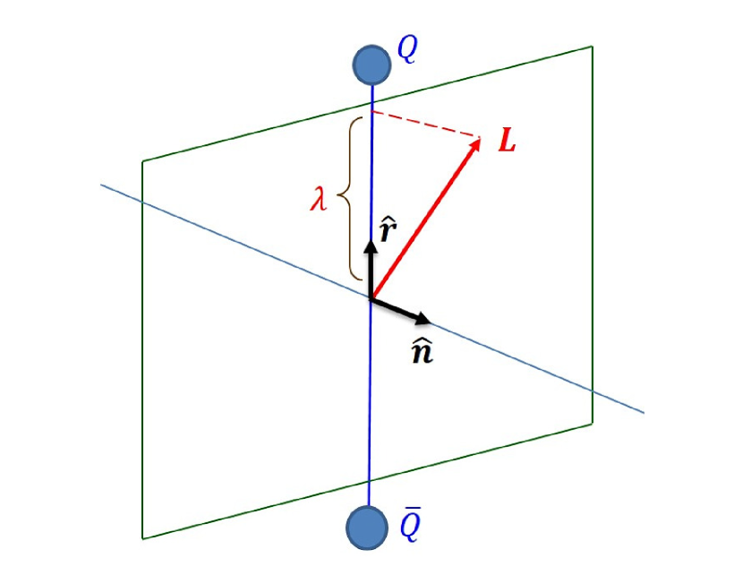
Figure 1: Symmetry directions and quantum numbers relevant to a “diatomic” ${Q\bar{Q}}$ system. The system is “homonuclear” when $Q$ and $\bar{Q}$, or $\delta$ and $\bar{\delta}$, are antiparticles of each other, and “heteronuclear” otherwise.

Since the BO potentials in the two-heavy-source case depend only upon $r$, the potentials connecting the $\delta^{\vphantom{1}}$-${\bar{\delta}}$ pair can be labeled by the irreducible representations of $D_{\infty h}$. The conventional quantum numbers used Landau and Lifshitz (1977) are $\Gamma\!\equiv\!\Lambda^{\epsilon}_{\eta}$. $\Lambda$ is an angular momentum projection, and $\epsilon$ and $\eta$ are inversion parities. With reference to Fig. 1, one defines a plane containing the axis $\hat{\bf r}$ and a unit normal $\hat{\bf n}$ to the plane. Denoting the total angular momentum of the light d.o.f.—a conserved quantity, thanks to the decoupling in the BO approximation—as $\bm{J}_{\rm light}$, and the orbital angular momentum of the heavy d.o.f. as $\bm{L}_{Q\bar{Q}}$, one obtains the total orbital angular momentum of the system,

$$\bm{L}\equiv\bm{L}_{Q\bar{Q}}+\bm{J}_{\rm light}\,.$$ (18)

Since $\hat{\bm{r}}\!\cdot\!\bm{L}_{Q\bar{Q}}=0$, the axial angular momentum $\hat{\bm{r}}\!\cdot\!\bm{J}_{\rm light}\!=\hat{\bm{r}}\!\cdot\!\bm{L}$ of the light d.o.f. is a good quantum number for the whole system, and its eigenvalues are denoted by $\lambda=0,\pm 1,\pm 2,\ldots$. One further notes that

$$L\geq|\hat{\bm{r}}\cdot\bm{L}|=|\hat{\bm{r}}\cdot\bm{J}_{\rm light}|=|\lambda|\equiv\Lambda\,.$$ (19)

Analogous to the use of labels $S,P,D,\ldots$ for the quantum numbers $L=0,1,2,\ldots$, one denotes potentials with the eigenvalues $\Lambda=0,1,2,\ldots$ by $\Sigma,\Pi,\Delta,\ldots$.

Reflection $R_{\rm light}$ of the light d.o.f. through the plane with unit normal $\hat{\bf n}$ (which is spatial inversion $P_{\rm light}$ of the light d.o.f., combined with a rotation by $\pi$ radians about $\hat{\bf n}$ originating from the $\delta^{\vphantom{1}}$-${\bar{\delta}}$ midpoint) transforms $\lambda\!\to\!-\lambda$. Since a glance at Fig. 1 reveals that the physical system (and hence its energy) must be invariant under $R_{\rm light}$, one finds that the energy eigenvalues must be a function only of $\Lambda\!\equiv\!|\lambda|$.

The eigenvalues of $R_{\rm light}$ itself are denoted $\epsilon\!=\!\pm 1$. Strictly speaking, specifying $\epsilon$ is essential only for $\Sigma$ potentials, for which the $\epsilon\!=\!\pm 1$ states may have distinct energies; however, one may also form $\epsilon$ eigenstates for (degenerate) $\Lambda\!>\!0$ BO potentials in the same way as one uses linear combinations of $f(+x)$ and $f(-x)$ to form both even and odd functions from an arbitrary function $f$. Following this procedure Lebed (2017), one obtains BO potentials for all values of $\Lambda^{\epsilon}$, in which case one also finds $P_{\rm light}\!=\!\epsilon(-1)^{\Lambda}$ in the “homonuclear” case.

Even for the “homonuclear” system, a complete inversion of coordinates of the light d.o.f. through the midpoint of the ${Q\bar{Q}}$ pair does not by itself produce an equivalent state to the original; rather, one must also exchange the ${Q\bar{Q}}$ pair, or instead, perform charge conjugation $C_{\rm light}$ upon the light d.o.f.  Thus, the full system in the “homonuclear” case is physically invariant under the combination $(CP)_{\rm light}$, and its eigenvalues $\eta\!=\!+1,-1$ are labeled as $g$, $u$, respectively.

In total, the three eigenvalues $\Lambda^{\epsilon}_{\eta}$ completely specify the irreducible representation of $D_{\infty h}$ for any “homonuclear diatomic” system. In the “heteronuclear diatomic” case (such as $B_{c}$ tetraquarks or the triquark-diquark pentaquark), the $(CP)_{\rm light}$ symmetry is lost (leaving the symmetry group $C_{\infty v}$), but the good quantum numbers $\Gamma\!\equiv\!\Lambda^{\epsilon}$ remain.

Appendix B Computational Methods

For both $n$-fold coupled and uncoupled reduced radial Schrödinger equations, one must solve a Sturm-Liouville problem of the form

$$\left[\mathbb{I}\frac{\textrm{d}^{2}}{\textrm{d}r^{2}}+\mathbf{Q}(r)\right]\!u(r)=0\,,$$ (20)

such that

$$\mathbf{Q}(r)\equiv\frac{2\mu}{\hbar^{2}}\left(E\,\mathbb{I}-\frac{\hat{\mathbf{L}}^{2}}{2\mu r^{2}}-\mathbf{V}(r)\right)\ \ \textrm{and}\ u(0)=0\,,$$ (21)

where $u$ is an $n$-dimensional column vector, $\mathbb{I}$ is an $n\times n$ identity matrix, $\hat{\mathbf{L}}^{2}$ is a matrix representing the angular momentum operator of the coupled system, $\mathbf{V}(r)$ is the interaction potential matrix, and $E$ is the energy eigenvalue of the Hamiltonian. One now takes the $n$ linearly independent column-vector solutions to Eq. (20) and concatenates them into an $n\times n$ matrix $\mathbf{U}(r)$. One can then numerically integrate each $u_{m}(r)$ for $m\in\{1,2,...,n\}$ simultaneously, via the equivalent problem:

$$\left[\mathbb{I}\frac{\textrm{d}^{2}}{\textrm{d}r^{2}}+\mathbf{Q}(r)\right]\!\mathbf{U}(r)=\textbf{0}\,.$$ (22)

The Sturm-Liouville problem of Eqs. (20)–(21) has a solution for any $E\in\mathbb{R}$. Since the probabilistic interpretation of quantum mechanics requires that solutions to Eq. (22) must be well-behaved as well as normalizable, one must have that the solution asymptotically approaches zero in the $r\rightarrow\infty$ limit:

$$\lim_{r\rightarrow\infty}\mathbf{U}(r)\rightarrow\textbf{0}\,.$$ (23)

The values of $E$ for which Eq. (23) is satisfied exist in a countable set. These are the physical eigenvalues of $E$.

In the case that $n=1$, numerically finding the value of $E$ for which Eq. (23) holds is accomplished via the use of the nodal theorem of Sturm-Liouville systems. This theorem has been generalized to systems for which $n\geq 1$ Amann and Quittner (1995). The generalized nodal theorem allows one to find the physical eigenvalues of $E$ in Eq. (22) by using $\det\mathbf{U}(r)$, without explicitly monitoring the functional solution $\mathbf{U}(r)$, to check that Eq. (23) is satisfied.

If $n=1$, one is assured that all of the nodes of $\mathbf{U}(r)\to u(r)$ are located in the classically allowed region. Hence, it is important to know where the classical turning points are located. For $n>1$, one has multiple potentials, and hence regions for which some potentials may be in their classically allowed regions, while others may be in their classically forbidden regions.

To make the notion of a “classical turning point” well defined in the coupled case, one can solve for the roots of the eigenvalues of $-\mathbf{Q}(r)$ as functions of $r$. For the case where each potential has only one classically allowed region, the inner classical turning point is defined as the innermost root of any of the eigenvalues of $-\mathbf{Q}(r)$, and the outer classical turning point is defined as the outermost root of any of the eigenvalues of $-\mathbf{Q}(r)$. This definition of the classical turning points ensures that no nodes are missed in the counting procedure due to having skipped over a portion of the classically allowed region of one of the potentials. Moreover, such a definition is established through multichannel generalizations of the WKB approximation Johnson (1973).

To find the desired value energy eigenvalue $E_{N}$ for which the solution $\mathbf{U}_{N}$ has $N$ nodes, one first chooses a window of $E$ values that is bounded below by $E_{\textrm{low}}$, bounded above by $E_{\textrm{high}}$, and that contains $E_{N}$. One then counts the number of nodes $\mathcal{N}$ of $\det\mathbf{U}(r)$ in the classically allowed region by numerically integrating Eq. (22) at $E=E_{\textrm{mid}}=(E_{\textrm{low}}+E_{\textrm{high}})/2$. Once the outer bound has been reached, one then sets $E_{\textrm{low}}=E_{\textrm{mid}}$ if $\mathcal{N}\leq N$, or sets $E_{\textrm{high}}=E_{\textrm{mid}}$ if $\mathcal{N}>N$. This procedure is repeated until $E_{\textrm{high}}-E_{\textrm{low}}$ meets a pre-specified tolerance.

B.1 Renormalized Numerov Integration Procedure

We now derive the renormalized Numerov method of Ref. Johnson (1978). Discretize the radial coordinate $r$ such that the initial value $r_{0}$ is located to the left of the inner classical turning point and is sufficiently close to the origin, while the final value $r_{f}$ is located sufficiently to the right of the outer classical turning point. Moreover, choose the grid to be uniformly spaced, with $r_{i+1}-r_{i}=h$ for all $i\in\{0,1,2,...,f\}$, and $h$ some arbitrarily small real number. Moreover, let $\mathbf{U}(r_{i})\equiv\mathbf{U}_{i}$.

Numerical integration of Eq. (22) can be accomplished by a coupled generalization of the Numerov recurrence relation:

$$\left(\mathbb{I}-\mathbf{T}_{i+2}\right)\mathbf{U}_{i+2}-\left(2\mathbb{I}+10\mathbf{T}_{i+1}\right)\mathbf{U}_{i+1}+\left(\mathbb{I}-\mathbf{T}_{i}\right)\mathbf{U}_{i}=\textbf{0}\,,$$ (24)

where

$$\mathbf{T}_{i}\equiv-\frac{h^{2}}{12}\mathbf{Q}(r_{i})\,.$$ (25)

The recurrence relation of the renormalized Numerov scheme results from three substitutions:

$$\mathbf{F}_{i} \equiv \left(\mathbb{I}-\mathbf{T}_{i}\right)\mathbf{U}_{i}\,,$$

$$\mathbf{H}_{i} \equiv \left(2\mathbb{I}+10\mathbf{T}_{i}\right)\left(\mathbb{I}-\mathbf{T}_{i}\right)^{-1}\,,$$

$$\mathbf{R}_{i} \equiv \mathbf{F}_{i+1}\mathbf{F}^{-1}_{i}\,.$$ (26)

The first two substitutions turn Eq. (24) into

$$\mathbf{F}_{i+2}-\mathbf{H}_{i+1}\mathbf{F}_{i+1}+\mathbf{F}_{i}=0\,,$$ (27)

and the last substitution renormalizes Eq. (27) as

$$\mathbf{R}_{i+1}=\mathbf{H}_{i+1}-\mathbf{R}^{-1}_{i}\,.$$ (28)

Equation (28) provides a stable and efficient method for propagating $\mathbf{U}_{i}$ in regions where the entries of $\mathbf{Q}$ diverge to $\pm\infty$, since $\mathbf{R}_{i}\sim\mathbf{Q}_{i+1}\mathbf{Q}^{-1}_{i}$. In most situations, one can choose $\mathbf{R}_{0}^{-1}=\mathbf{0}$; however, this choice can present complications Johnson (1978). We instead set $\mathbf{R}^{-1}_{0}$ to be

$$\mathbf{R}^{-1}_{0}=\left(\mathbb{I}-\mathbf{T}_{0}\right)\left(2\mathbb{I}+10\mathbf{T}_{0}\right)^{-1}=\mathbf{H}_{0}^{-1}\,.$$ (29)

If $r_{0}=h$, then this choice is equivalent to supposing that $\mathbf{R}_{-1}^{-1}=\mathbf{0}$ precisely at the origin, $r=r_{-1}=0$.

We now describe a method for counting the number of nodes along the integration without explicitly monitoring $\det\mathbf{U}_{i}$ at each integration step. First suppose that there is only one node of $\det\mathbf{U}$ between $r_{i+1}$ and $r_{i}$. From the last of Eq. (B.1), one has that

$$\det\mathbf{R}_{i+1}=\frac{\det(\mathbb{I}-\mathbf{T}_{i+1})}{\det(\mathbb{I}-\mathbf{T}_{i})}\times\frac{\det\mathbf{U}_{i+1}}{\det\mathbf{U}_{i}}\,.$$ (30)

Since $\det(\mathbb{I}-\mathbf{T}_{i+1})>0$ for any $r_{i}$ in the classically allowed region, one has that $\det\mathbf{R}_{i+1}<0$, since $\det\mathbf{U}$ encountering one node between $r_{i+1}$ and $r_{i}$ implies that $\det\mathbf{U}_{i}$ and $\det\mathbf{U}_{i+1}$ have opposite signs. It follows that one may monitor $\det\mathbf{R}_{i}$ at each integration step to count the number of nodes. Such a method is effective if only one node exists between each pair of grid points, as the existence of even numbers of nodes between any two grid points (due to degeneracies, for example) implies that $\det\mathbf{U}_{i+1}$ and $\det\mathbf{U}_{i}$ have the same sign, and hence $\det\mathbf{R}_{i+1}>0$.

One can avoid missing nodes by instead monitoring the individual eigenvalues of $\mathbf{R}_{i}$ at each integration point. If $\det\mathbf{R}_{i}<0$, then there is an odd number of negative eigenvalues. However, if $\det\mathbf{R}_{i}>0$, there is an even number of negative eigenvalues, and an incorrect node count occurs. Therefore, if one instead monitors each time one of the eigenvalues of $\mathbf{R}_{i}$ changes sign, there is no danger of missing a node. This procedure is equivalent to monitoring the signature of $\mathbf{R}_{i}$, and one can therefore equivalently count the number of times one of the diagonal entries of the $U$ matrix in an $LU$-decomposition of $\mathbf{R}_{i}$ changes sign.

B.2 Calculation of Expectation Values

From nondegenerate perturbation theory, one learns that if the Hamiltonian $H$ splits into some reference Hamiltonian $H^{(0)}$ and a small perturbation $\epsilon H^{\prime}$, then the energy eigenvalues can be calculated perturbatively. To first order in $\epsilon$, this perturbative expansion is:

$$E^{\prime}_{N}=E^{(0)}_{N}+\epsilon\langle N|H^{\prime}|N\rangle+\mathcal{O}\left(\epsilon^{2}\right)\,.$$ (31)

The expectation value of $H^{\prime}$ is then found as the limit

$$\langle N|H^{\prime}|N\rangle=\lim_{\epsilon\rightarrow 0}\frac{E_{N}^{\prime}-E^{(0)}_{N}}{\epsilon}\,.$$ (32)

While this result when $H^{\prime}$ is specifically a Hamiltonian perturbation is the conventional Feynman-Hellmann theorem, it remains true for any Hermitian operator $H^{\prime}$. Therefore, Eq. (32) provides a method Hutson (1994) for numerically calculating the expectation values of arbitrary operators using just the energy eigenvalues of the original problem and the energy eigenvalues of Eq. (31), so long as these energies are non-degenerate. This observation is very powerful, because it means that one does not need to numerically compute the wave functions of Eq. (22) in the calculation of expectation values.

References

- Lebed et al. (2017) R. Lebed, R. Mitchell, and E. Swanson, Prog. Part. Nucl. Phys. 93, 143 (2017), arXiv:1610.04528 [hep-ph] .
- Chen et al. (2016) H.-X. Chen, W. Chen, X. Liu, and S.-L. Zhu, Phys. Rept. 639, 1 (2016), arXiv:1601.02092 [hep-ph] .
- Hosaka et al. (2016) A. Hosaka, T. Iijima, K. Miyabayashi, Y. Sakai, and S. Yasui, Prog. Theor. Exp. Phys. 2016, 062C01 (2016), arXiv:1603.09229 [hep-ph] .
- Esposito et al. (2016) A. Esposito, A. Pilloni, and A. Polosa, Phys. Rept. 668, 1 (2016), arXiv:1611.07920 [hep-ph] .
- Guo et al. (2018) F.-K. Guo, C. Hanhart, U.-G. Meißner, Q. Wang, Q. Zhao, and B.-S. Zou, Rev. Mod. Phys. 90, 015004 (2018), arXiv:1705.00141 [hep-ph] .
- Ali et al. (2017) A. Ali, J. Lange, and S. Stone, Prog. Part. Nucl. Phys. 97, 123 (2017), arXiv:1706.00610 [hep-ph] .
- Olsen et al. (2018) S. Olsen, T. Skwarnicki, and D. Zieminska, Rev. Mod. Phys. 90, 015003 (2018), arXiv:1708.04012 [hep-ph] .
- Karliner et al. (2018) M. Karliner, J. Rosner, and T. Skwarnicki, Ann. Rev. Nucl. Part. Sci. 68, 17 (2018), arXiv:1711.10626 [hep-ph] .
- Yuan (2018) C.-Z. Yuan, Int. J. Mod. Phys. A33, 1830018 (2018), arXiv:1808.01570 [hep-ex] .
- Maiani et al. (2005) L. Maiani, F. Piccinini, A. Polosa, and V. Riquer, Phys. Rev. D 71, 014028 (2005), arXiv:hep-ph/0412098 [hep-ph] .
- Maiani et al. (2014) L. Maiani, F. Piccinini, A. Polosa, and V. Riquer, Phys. Rev. D 89, 114010 (2014), arXiv:1405.1551 [hep-ph] .
- Anselmino et al. (1993) M. Anselmino, E. Predazzi, S. Ekelin, S. Fredriksson, and D. Lichtenberg, Rev. Mod. Phys. 65, 1199 (1993).
- Brodsky et al. (2014) S. Brodsky, D. Hwang, and R. Lebed, Phys. Rev. Lett. 113, 112001 (2014), arXiv:1406.7281 [hep-ph] .
- Brodsky and Lebed (2015) S. Brodsky and R. Lebed, Phys. Rev. D 91, 114025 (2015), arXiv:1505.00803 [hep-ph] .
- Lebed (2015) R. Lebed, Phys. Lett. B 749, 454 (2015), arXiv:1507.05867 [hep-ph] .
- Lebed (2017) R. Lebed, Phys. Rev. D 96, 116003 (2017), arXiv:1709.06097 [hep-ph] .
- Eichten et al. (1978) E. Eichten, K. Gottfried, T. Kinoshita, K. Lane, and T.-M. Yan, Phys. Rev. D 17, 3090 (1978), [Erratum: Phys. Rev. D 21, 313 (1980)].
- Eichten et al. (1980) E. Eichten, K. Gottfried, T. Kinoshita, K. Lane, and T.-M. Yan, Phys. Rev. D 21, 203 (1980).
- Born and Oppenheimer (1927) M. Born and R. Oppenheimer, Ann. der Phys. 389, 457 (1927).
- Griffiths et al. (1983) L. Griffiths, C. Michael, and P. Rakow, Phys. Lett. 129B, 351 (1983).
- Berwein et al. (2015) M. Berwein, N. Brambilla, J. Tarrús Castellà, and A. Vairo, Phys. Rev. D 92, 114019 (2015), arXiv:1510.04299 [hep-ph] .
- Lebed and Swanson (2018) R. Lebed and E. Swanson, Few Body Syst. 59, 53 (2018), arXiv:1708.02679 [hep-ph] .
- Juge et al. (1998) K. Juge, J. Kuti, and C. Morningstar, Contents of LAT97 proceedings, Nucl. Phys. Proc. Suppl. 63, 326 (1998), arXiv:hep-lat/9709131 [hep-lat] .
- Juge et al. (1999) K. Juge, J. Kuti, and C. Morningstar, Phys. Rev. Lett. 82, 4400 (1999), arXiv:hep-ph/9902336 [hep-ph] .
- Juge et al. (2003) K. Juge, J. Kuti, and C. Morningstar, Phys. Rev. Lett. 90, 161601 (2003), arXiv:hep-lat/0207004 [hep-lat] .
- (26) http://www.andrew.cmu.edu/user/cmorning/static_potentials/SU3_4D/greet.html.
- Capitani et al. (2019) S. Capitani, O. Philipsen, C. Reisinger, C. Riehl, and M. Wagner, Phys. Rev. D 99, 034502 (2019), arXiv:1811.11046 [hep-lat] .
- Bali and Pineda (2004) G. Bali and A. Pineda, Phys. Rev. D 69, 094001 (2004), arXiv:hep-ph/0310130 [hep-ph] .
- Bicudo et al. (2017) P. Bicudo, M. Cardoso, O. Oliveira, and P. Silva, Phys. Rev. D 96, 074508 (2017), arXiv:1702.07789 [hep-lat] .
- Braaten (2013) E. Braaten, Phys. Rev. Lett. 111, 162003 (2013), arXiv:1305.6905 [hep-ph] .
- Braaten et al. (2014a) E. Braaten, C. Langmack, and D. Smith, Phys. Rev. Lett. 112, 222001 (2014a), arXiv:1401.7351 [hep-ph] .
- Braaten et al. (2014b) E. Braaten, C. Langmack, and D. Smith, Phys. Rev. D 90, 014044 (2014b), arXiv:1402.0438 [hep-ph] .
- Aubert and et al. (2005) B. Aubert and et al. (BaBar Collaboration), Phys. Rev. D 71, 031501 (2005), arXiv:hep-ex/0412051 [hep-ex] .
- Aaij and et al. (2019) R. Aaij and et al. (LHCb Collaboration), (2019), arXiv:1904.03947 [hep-ex] .
- Caswell and Lepage (1986) W. Caswell and G. Lepage, Phys. Lett. 167B, 437 (1986).
- Bodwin et al. (1995) G. Bodwin, E. Braaten, and G. Lepage, Phys. Rev. D 51, 1125 (1995), [Erratum: Phys. Rev. D 55,5853 (1997)], arXiv:hep-ph/9407339 [hep-ph] .
- Pineda and Soto (1998) A. Pineda and J. Soto, Quantum Chromodynamics. Proceedings, Conference, QCD’97, Montpellier, France, July 3–9, 1997, Nucl. Phys. Proc. Suppl. 64, 428 (1998), arXiv:hep-ph/9707481 [hep-ph] .
- Brambilla et al. (2000) N. Brambilla, A. Pineda, J. Soto, and A. Vairo, Nucl. Phys. B566, 275 (2000), arXiv:hep-ph/9907240 [hep-ph] .
- Landau and Lifshitz (1977) L. Landau and E. Lifshitz, Quantum Mechanics: Non-Relativistic Theory, Course of Theoretical Physics (Pergamon Press, Oxford, U.K., 1977).
- Johnson (1978) B. Johnson, J. Chem. Phys. 69, 4678 (1978).
- Hutson (1994) J. Hutson, Comp. Phys. Comm. 84, 1 (1994).
- Barnes et al. (2005) T. Barnes, S. Godfrey, and E. Swanson, Phys. Rev. D 72, 054026 (2005), arXiv:hep-ph/0505002 [hep-ph] .
- Tanabashi and et al. (2018) M. Tanabashi and et al. (Particle Data Group), Phys. Rev. D 98, 030001 (2018).
- Lebed and Polosa (2016) R. Lebed and A. Polosa, Phys. Rev. D 93, 094024 (2016), arXiv:1602.08421 [hep-ph] .
- Aaij and et al. (2018) R. Aaij and et al. (LHCb Collaboration), Eur. Phys. J. C78, 1019 (2018), arXiv:1809.07416 [hep-ex] .
- Zhou et al. (2015) Z.-Y. Zhou, Z. Xiao, and H.-Q. Zhou, Phys. Rev. Lett. 115, 022001 (2015), arXiv:1501.00879 [hep-ph] .
- Chilikin and et al. (2017) K. Chilikin and et al. (Belle Collaboration), Phys. Rev. D 95, 112003 (2017), arXiv:1704.01872 [hep-ex] .
- Ablikim and et al. (2017a) M. Ablikim and et al. (BESIII Collaboration), Phys. Rev. D 96, 032004 (2017a), [Erratum: Phys. Rev. D 99, 019903 (2019)], arXiv:1703.08787 [hep-ex] .
- Ablikim and et al. (2018) M. Ablikim and et al. (BESIII Collaboration), Phys. Rev. D 97, 052001 (2018), arXiv:1710.10740 [hep-ex] .
- Yuan and et al. (2007) C.-Z. Yuan and et al. (Belle Collaboration), Phys. Rev. Lett. 99, 182004 (2007), arXiv:0707.2541 [hep-ex] .
- Ablikim and et al. (2017b) M. Ablikim and et al. (BESIII Collaboration), Phys. Rev. Lett. 118, 092002 (2017b), arXiv:1610.07044 [hep-ex] .
- Bulava et al. (2019) J. Bulava, B. Hörz, F. Knechtli, V. Koch, G. Moir, C. Morningstar, and M. Peardon, (2019), arXiv:1902.04006 [hep-lat] .
- Giron et al. (2019) J. Giron, R. Lebed, and C. Peterson, (2019), in preparation.
- Cleven et al. (2015) M. Cleven, F.-K. Guo, C. Hanhart, Q. Wang, and Q. Zhao, Phys. Rev. D 92, 014005 (2015), arXiv:1505.01771 [hep-ph] .
- Alford et al. (1999) M. Alford, K. Rajagopal, and F. Wilczek, Nucl. Phys. B537, 443 (1999), arXiv:hep-ph/9804403 [hep-ph] .
- Amann and Quittner (1995) H. Amann and P. Quittner, J. Math. Phys. 36, 4553 (1995).
- Johnson (1973) B. Johnson, Chem. Phys. 36, 381 (1973).