Universal entanglement decay of photonic orbital angular momentum qubit states in atmospheric turbulence: an analytical treatment

Abstract

We study the entanglement evolution of photonic orbital angular momentum qubit states with opposite azimuthal indices $l_{0}$, in a weakly turbulent atmosphere. Using asymptotic methods, we deduce analytical expressions for the amplitude of turbulence-induced crosstalk between the modes $l_{0}$ and $-l_{0}$. Furthermore, we analytically establish distinct, universal entanglement decay laws for Kolmogorov’s turbulence model and for two approximations thereof.

I Introduction

Helical wave fronts of twisted photons allow for encoding high-dimensional (qudit) states in the orbital angular momentum (OAM) degree of freedom that is characterized by an azimuthal index $l_{0}=0,\pm 1,\pm 2,\ldots$ Allen et al. (1992); Molina-Terriza et al. (2007); Franke-Arnold et al. (2008). Using qudit states can potentially ensure higher channel capacity Gibson et al. (2004); Barreiro et al. (2008) and enhanced security Bechmann-Pasquinucci and Peres (2000); Bourennane et al. (2001) of quantum communication channels as compared to two-dimensional, polarization-based, encoding. So far, the full-scale use of twisted photons in free space quantum communication has remained elusive due to the sensitivity of the photons’ wave fronts with respect to intrinsic fluctuations of the refractive index of air (atmospheric turbulence) Tatarskii (1961). Notwithstanding, recent experimental progress where OAM encoding was used in free space quantum key distribution over up to 300 m Vallone et al. (2014); Sit et al. (2017), for entanglement distribution over 3 km Krenn et al. (2015), and for the transmission of classical twisted light over 143 km Krenn et al. (2016), indicates that turbulence-induced phase-front distortions do not in principle preclude the reliable transfer of twisted photons through the atmosphere. Yet, we still lack a complete understanding of the behaviour of photonic OAM states in turbulence, even for OAM-encoded qubits.

Since one of the most prominent quantum communication protocols Ekert (1991) is based on quantum entanglement Mintert et al. (2005); Horodecki et al. (2009) – which is readily generated between OAM states in the lab Mair et al. (2001); Fickler et al. (2012); van Exter et al. (2012) – experimental Pors et al. (2011); Hamadou Ibrahim et al. (2013); Zhang et al. (2016); Goyal et al. (2016); Ndagano et al. (2017) and theoretical Gopaul and Andrews (2007); Sheng et al. (2012); Roux (2011); Ibrahim et al. (2014); Roux et al. (2015); Roux (2017) efforts explore how entanglement of twisted biphotons decoheres in the atmosphere. In particular, it was predicted Smith and Raymer (2006) – and recently confirmed experimentally Hamadou Ibrahim et al. (2013) – that entangled qubit states with opposite OAM become more robust in weak turbulence as the azimuthal index $l_{0}$ increases.

Some useful insight into this feature was provided through the introduction of the phase correlation length $\xi(l_{0})$ Leonhard et al. (2015) that is the characteristic length scale associated with the transverse spatial structure of OAM beams. In particular, it was numerically shown Leonhard et al. (2015) that the individual temporal evolution of the concurrence Mintert et al. (2005); Wootters (1998) of initially maximally entangled OAM qubit states with quantum numbers $\pm l_{0}$ collapses onto an $l_{0}$-independent, universal entanglement decay, upon rescaling the turbulence strength by $\xi(l_{0})$. However, no analytical derivation of this universal decay law has so far been available.

In the present contribution, we revisit the entanglement evolution of photonic OAM qubit states in weak turbulence and generalize the results of Leonhard et al. (2015) along two directions: First, we deduce the entanglement decay law analytically. To this end, we exploit the universality of the decay, and consider the limit $l_{0}\gg 1$, using asymptotic methods. Second, we derive explicit expessions for the universal decay law for three distinct models of turbulence – distinguished by the exponent $\alpha$ of the phase structure function Tatarskii (1961); Andrews and Phillips (2005) (see Sec. II). This generalization is inspired by the fact that the universal form of the entanglement decay relies on the weakness of the turbulence. The latter assumption implies that the impact of turbulence on the propagated wave can be described by a single phase screen Buckley (1975), irrespective of the specific turbulence model. Since variation of $\alpha$ leads to different types of atmospheric disorder, it is interesting to explore, somewhat in the spirit of Kropf et al. (2016), how this affects entanglement evolution in turbulence.

The paper is structured as follows: In the next section we present our general model of turbulence, parametrized by the exponent $\alpha$, as well as our method to access the entanglement evolution. In Sec. III we derive explicit expressions for the relative crosstalk amplitude, $\tilde{b}$, in the asymptotic limit $l_{0}\gg 1$, for $\alpha=1,5/3,2$, and compare these asymptotic results to numerically exact data. We finally give analytic formulations for the universal entanglement decay law, for those different values of $\alpha$. Section IV concludes the manuscript.

II Model

We consider a maximally entangled OAM qubit state of two photons, encoded in two Laguerre-Gauss (LG) modes with radial and azimuthal quantum numbers $p=0$ and $l=\pm l_{0}$, respectively, and relative phase $\varphi$:

$$|\psi_{0}\rangle=\frac{1}{\sqrt{2}}(|l_{0}\rangle|-l_{0}\rangle+e^{i\varphi}|-l_{0}\rangle|l_{0}\rangle),$$ (1)

Such states can be generated experimentally Mair et al. (2001); van Exter et al. (2012), and large values up to $l_{0}=300$ were reported Fickler et al. (2012). The entangled photons are sent, in opposite directions along the (horizontal) $z$-axis, through the atmosphere and the impact of the latter on the transmitted photons is modelled by two independent phase screens — one for each photon. This model of atmospheric turbulence ignores turbulence-induced intensity fluctuations. Furthermore, we neglect diffraction, assuming that the widths of the LG beams remain constant along the propagation paths. As follows from Paterson (2004), both assumptions are valid for short propagation distances of about one km for each photon. Note that this is a standard approach Andrews and Phillips (2005) which only accounts for scattering of an optical wave on refractive index inhomogeneities of a typical scale much larger than the optical wave length. This model does therefore not describe any loss of information as induced, e.g., by photon absorption, Rayleigh scattering by air molecules, or Mie scattering by aerosols. These processes, however, only affect the total transmission rate of the photons, but leave the description of the atmospheric imprint on the successfully transmitted photons invariant.

When a pair of twisted photons prepared in state (1) is sent across the atmosphere, turbulence-induced random phase shifts lead to the coupling, or crosstalk, of the initially excited (LG${}_{0\pm l_{0}}$) modes to other LG_pl modes, spreading, in general, over infinitely many values of $p$ and of $l$. Upon averaging this high-dimensional pure state over independent statistical realizations of those random shifts, one ends up with a mixed state.

Thus, the output biphoton state $\varrho$ can be described by a map Leonhard et al. (2015)

$$\varrho=(\Lambda_{1}\otimes\Lambda_{2})\varrho_{0},$$ (2)

where $\Lambda_{i}$ is the disorder-averaged turbulence map acting on the state of the $i$th photon, and $\varrho_{0}=|\psi_{0}\rangle\langle\psi_{0}|$. The tensor product expresses the independence of the action of the two screens on either photon.

Since we are only interested in the OAM entanglement evolution in the subspace of the initially populated OAM modes, we trace over the radial quantum number $p$, and project the output state onto the subspace spanned by the four product vectors: $|l_{0}\rangle|l_{0}\rangle,|l_{0}\rangle|-l_{0}\rangle,|-l_{0}\rangle|l_{0}\rangle,|-l_{0}\rangle|-l_{0}\rangle$ Leonhard et al. (2015). Due to the projection, the norm of the resulting state is reduced and the state needs to be renormalized by its trace Bertlmann et al. (2003). The entanglement evolution of the thereby obtained mixed, bipartite qubit state can be evaluated using Wootter’s concurrence Wootters (1998).

The elements of the map $\Lambda_{i}$ required for the evaluation of the output state $\varrho$ are given by (see A)

$$\Lambda_{l,\pm l}^{0,l_{0},0,l_{0}^{\prime}} =\frac{1}{2\pi}\delta_{l_{0}-l_{0}^{\prime},l\pm l}\int_{0}^{\infty}\int_{0}^{2\pi}r\mathrm{d}r\mathrm{d}\vartheta$$

$$\times R_{0,l_{0}}(r)R_{0,l_{0}^{\prime}}(r)e^{-i\frac{\vartheta}{2}[(l\pm l)-(l_{0}+l_{0}^{\prime})]}$$

$$\exp\left\{-\frac{1}{2}D_{\phi}\left[2r\sin\left(\frac{\vartheta}{2}\right)\right]\right\},$$ (3)

where upper and lower indices of $\Lambda_{l,\pm l}^{0,l_{0},0,l_{0}^{\prime}}$ correspond to the input and output states, respectively, $\delta_{l_{0}-l_{0}^{\prime},l\pm l}$ is the Kronecker delta,

$$R_{0,l_{0}}(r)=\frac{2}{\sqrt{|l_{0}|!}}\frac{1}{w_{0}}\left(\frac{\sqrt{2}r}{w_{0}}\right)^{|l_{0}|}\,e^{-r^{2}/w_{0}^{2}},$$ (4)

is the radial part of the LG${}_{0\pm l_{0}}$ mode at $z=0$, with $p=0$, $l=\pm l_{0}$, and $w_{0}$ is the mode’s width. Furthermore,

$$D_{\phi}(x)=\gamma\left(\frac{x}{r_{0}}\right)^{\alpha}$$ (5)

is the phase structure function of turbulence, which determines the statistics of the spatial wavefront deformations Fried (1965). Here, $\gamma=6.88$ and

$$r_{0}=(0.423\,C_{n}^{2}k^{2}L)^{-3/5}$$ (6)

is the Fried parameter Fried (1966); Andrews and Phillips (2005), with $C_{n}^{2}$ the index-of-refraction structure constant, $k$ the optical wave number, and $L$ the propagation distance. Throughout this work, we assume that both photons traverse equal-length paths in the atmosphere characterized by the same $C_{n}^{2}$. Hence, $r_{0}$ coincides for both screens.

The exponent $\alpha$ in Eq. (5) specifies the turbulence model. In particular, $\alpha=5/3$ characterizes Kolmogorov’s description Tatarskii (1961); Andrews and Phillips (2005), but we subsequently also consider the entanglement evolution for $\alpha=1,2$ which can be regarded as integer-value “approximations” of $\alpha=5/3$. In fact, the phase structure function with $\alpha=2$ is oftentimes used in the literature Smith and Raymer (2006); Roux (2017); Roux et al. (2015); Ndagano et al. (2017), with Eq. (5) then called the “quadratic approximation” Leader (1978) of the Kolmogorov phase structure function (by analogy, we refer to the case $\alpha=1$ as the “linear approximation”). Apart from the fact that the quadratic approximation allows for obtaining analytical results for entanglement decay of OAM qubit states even under conditions of strong turbulence Roux et al. (2015); Roux (2017), it is sometimes considered to be slightly pessimistic Chandrasekaran and Shapiro (2014) as compared to the Kolmogorov model. Indeed, as follows from Eqs. (3) and (5), the matrix elements of the map $\Lambda_{i}$ governing the evolution of the density operator will decay faster with $x$ for $\alpha=2$ than for $\alpha=5/3$. Consequently, the first-order spatial correlation function of the propagated field (also known as the mutual coherence function Tatarskii (1961); Andrews and Phillips (2005)) decreases more rapidly within the square-law approximation, which is considered Chandrasekaran and Shapiro (2014) to be harmful for optical communication. However, as for the entanglement evolution of OAM states, a smaller magnitude of those matrix elements of $\Lambda_{i}$ that reflect the coupling between OAM modes with $-l_{0}$ and $l_{0}$ is actually useful, because it is the intermodal crosstalk that causes entanglement decay Leonhard et al. (2015).

As a result, as we show in this work, the robustness of entanglement is most pronounced for $\alpha=2$. From this viewpoint, the quadratic approximation appears as overly optimistic. Consistently, the linear approximation, $\alpha=1$, yields pessimistic results as compared to those derived from the Kolmogorov model.

III Universal entanglement decay laws

III.1 General expressions

Upon application of the turbulence map (2), the output state’s concurrence is given analytically by Leonhard et al. (2015)

$$C(\varrho)=\max\left[0,\frac{1-2\tilde{b}}{(1+\tilde{b})^{2}}\right],$$ (7)

where $\tilde{b}=b/a$ is the reduced, or relative, crosstalk amplitude, with

$$a=\Lambda^{l_{0},l_{0}}_{l_{0},l_{0}} =\Lambda^{-l_{0},-l_{0}}_{-l_{0},-l_{0}}=\Lambda^{-l_{0},l_{0}}_{-l_{0},l_{0}}=\Lambda^{l_{0},-l_{0}}_{l_{0},-l_{0}},$$ (8a)

$$b =\Lambda^{-l_{0},-l_{0}}_{l_{0},l_{0}}=\Lambda^{l_{0},l_{0}}_{-l_{0},-l_{0}},$$ (8b)

expressed in terms of the phase screen map’s matrix elements (3) (we drop their upper indices $p=0$ for brevity). We note that Eq. (7) is valid for a single phase screen description of turbulence, whereas the specific turbulence model is included via the dependence of the parameters $a$ and $b$ on $\alpha$. As follows from the definition (3), in the absence of turbulence, or, equivalently, when $r_{0}\rightarrow\infty$, the survival amplitude tends to one, $a\rightarrow 1$, while $b\rightarrow 0$, for the crosstalk amplitude. Hence, also $\tilde{b}\rightarrow 0$, and concurrence converges to its maximum value of unity. In contrast, when turbulence comes into play, crosstalk between different OAM modes is expected, and $C(\varrho)$ given by (7) should thus drop below unity. As we show below, this expectation is not always justified.

In the framework of the Kolmogorov model of turbulence, by numerical assessment of $a$ and $b$, we established earlier that the behaviour of $C(\varrho)$ is universal in the sense that the a priori $l_{0}$-dependent entanglement evolution with the penetration depth into the turbulent medium collapses onto one universal curve, for arbitrary OAM $l_{0}>1$, provided $C(\varrho)$ is considered as a function of the rescaled turbulence strength $\xi(l_{0})/r_{0}$ Leonhard et al. (2015). Here, $\xi(l_{0})$ is the phase correlation length of an LG${}_{0l_{0}}$ beam of width $w_{0}$, which reads Leonhard et al. (2015)

$$\xi(l_{0})=\sin\left(\frac{\pi}{2|l_{0}|}\right)\frac{w_{0}}{\sqrt{2}}\frac{\Gamma(|l_{0}|+3/2)}{\Gamma(|l_{0}|+1)}.$$ (9)

Thus, the entanglement evolution within the Kolmogorov and single phase screen model is determined by the ratio of the only two characteristic length scales, of which $\xi(l_{0})$ refers to the OAM beam and $r_{0}$ to the turbulent medium. In the following, we analytically show that the universality of the entanglement decay persists also for $\alpha=1$ and $\alpha=2$, though with a different functional form, which we identify for $\alpha=1,5/3,2$.

By virtue of Eq. (7), the universality of the concurrence decay law originates from that of the relative crosstalk amplitude, $\tilde{b}\equiv\tilde{b}(\xi(l_{0})/r_{0})$. Therefore, we need to infer the explicit form of the latter. To that end, we consider the limit $l_{0}\gg 1$, and apply asymptotic analysis. Using the method of steepest descent Carrier et al. (2005), we obtain the following expressions (see B):

$$a \approx\frac{1}{\pi}A^{-1/\alpha}\,\Gamma\left(1+\frac{1}{\alpha}\right),$$ (10)

$$b \approx\frac{1}{\pi}\,{\rm Re}\,\left[\int_{0}^{\infty}\mathrm{d}{x}\exp(-A\,x^{\alpha}-2il_{0}\,x)\right],$$ (11)

where $A=2^{-\alpha-1}\,\gamma\,(2l_{0})^{\alpha/2}\,t^{\alpha}$, and

$$t:=w_{0}/r_{0}$$ (12)

is the turbulence strength. The asymptotic solutions (10) and (11) essentially accomplish our target: Indeed, (10) already has an explicit analytical form. Equation (11) involves a highly oscillatory integral which, in turn, can be evaluated by asymptotic methods. Though, for any $\alpha=l/k$, with $l,k$ positive integers, Eq. (11) can be evaluated exactly and is given in terms of either elementary ($\alpha=1,2$) or of special ($\alpha=5/3$) functions. Next, we analyze these three cases in more detail.

Before proceeding, we would like to point out that any distinctions in the $l_{0}$- and $t$-dependencies of $\tilde{b}$ and, hence, of the entanglement decay laws, for different $\alpha$, can stem exclusively from the turbulence-induced crosstalk amplitude $b$. Indeed, as follows from our asymptotic expression (10), for any $1\leq\alpha\leq 2$, the survival amplitude $a\sim 1/t\sqrt{l_{0}}$. Finally, to study the behaviour of the survival amplitude for $0<t\ll 1$, using the approximate formula (10), the physical bounds $0<a\leq 1$ have to be kept in mind, and $l_{0}\gg 1$ needs to be chosen accordingly.

III.2 Asymptotic expressions for survival and crosstalk amplitudes

III.2.1 Linear approximation ($\alpha=1$)

For $\alpha=1$, (10) and (11) yield the following asymptotic results ($l_{0}\gg 1$):

$$a\approx\frac{4}{\pi\gamma}\frac{1}{\sqrt{2l_{0}}t},\quad b\approx\frac{\gamma}{4\pi}\frac{\sqrt{2l_{0}}t}{4l_{0}^{2}+\gamma^{2}t^{2}l_{0}/8}.$$ (13)

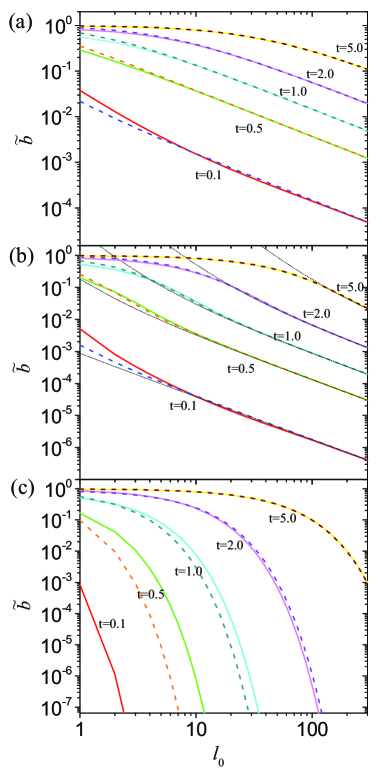
Figure 1: (Color online) Relative crosstalk amplitude $\tilde{b}$ versus the azimuthal index $l_{0}$ (on a log-log scale), for $t\equiv w_{0}/r_{0}=0.1,0.5,1.0,2.0,5.0$ and for three values of $\alpha$ [see Eq. (5)]: (a) $\alpha=1$, (b) $\alpha=5/3$, (c) $\alpha=2$. Solid lines indicate exact numerical integration of Eq. (3), dashed lines correspond to asymptotic expressions (a) (13), (b) (15), (c) (18). Thin dotted lines in panel (b) represent the asymptotic expansion (16).

In Fig. 1(a) we show the function $\tilde{b}=b/a$, as obtained by exact numerical evaluation of the integrals in Eq. (3), together with the asymptotic solution derived from Eq. (13). We notice that the asymptotic value of the ratio $b/a$ provides excellent agreement with the exact numerical solution already for $l_{0}\gtrsim 10$. As follows from Eq. (13), at leading order the relative crosstalk amplitude reads

$$\tilde{b}\sim\frac{\gamma^{2}t^{2}}{32l_{0}},$$ (14)

i.e., is proportional to $t^{2}/l_{0}$.

III.2.2 Kolmogorov turbulence ($\alpha=5/3$)

After a suitable coordinate transformation (see B), the integral in Eq. (11) reduces to a tabulated integral Prudnikov et al. (1992). Explicitly, the amplitudes $a$ and $b$ for $\alpha=5/3$ read:

$$a \approx\frac{\sqrt{2}(\gamma/2)^{-3/5}}{\pi t\sqrt{l_{0}}}\Gamma\left(\frac{8}{5}\right),$$ (15a)

$$b \approx\frac{\sqrt{15}}{2^{3}\pi^{4}}$$ (15b)

$$\times\,{\rm Re}\,\left[\frac{e^{-i\pi/5}}{s}G^{3,5}_{5,3}\left(\left.\frac{5^{5}q^{3}}{3^{3}s^{5}}\right|\begin{array}[]{lllll}0,&\frac{1}{5},&\frac{2}{5},&\frac{3}{5},&\frac{4}{5}\\ 0,&\frac{1}{3},&\frac{2}{3}&&\end{array}\right)\right],$$ (15e)

where $s=2il_{0}\,e^{-i\pi/5}$, $q=\gamma\,2^{-11/6}\,t^{5/3}\,l_{0}^{5/6}e^{-i\pi/3}$, and $G^{3,5}_{5,3}(x|\dots)$ is the Meijer G-function, which can be expressed through generalized hypergeometric functions Bateman (1953). As in the case $\alpha=1$, the numerically exact and the asymptotic results merge for $l_{0}\gtrsim 10$ (see Fig.  1(b)). However, the hypergeometric functions are a representation of an infinite series Abramowitz and Stegun (1964). A transparent analytical form of the dependence of $\tilde{b}$ on $l_{0}$ can be deduced from the asymptotic series expansion of $\tilde{b}$ which can be derived directly from (10,11). For a large value of a parameter (in our case, for $l_{0}\gg 1$) the subsequent terms of an asymptotic series first decrease in magnitude, but then start progressively increasing Dingle (1973). Thus, the asymptotic series are divergent. Nonetheless, these series are useful, since a finite number of terms of an asymptotic series expansion yields a very accurate representation of the function at large parameter values Dingle (1973). As regards the relative crosstalk amplitude $\tilde{b}$, its best approximation for $0.1\lesssim t\lesssim 5$ and $l_{0}\gtrsim 150$ is obtained by the first three terms of the asymptotic series (see Eqs. (61)-(68) in B):

$$\tilde{b} \approx 0.380\!\left(\!\frac{t^{2}}{l_{0}}\!\right)^{\!\!\frac{4}{3}}\!\!\!\!+\!1.231\!\left(\!\frac{t^{2}}{l_{0}}\!\right)^{\!\!\frac{13}{6}}\!\!\!\!\!\!+\!3.735\!\left(\!\frac{t^{2}}{l_{0}}\!\right)^{\!\!3}\!\!\!+\!O\!\!\left[\left(\!\frac{t^{2}}{l_{0}}\!\right)^{\!\frac{23}{6}}\right].$$ (16)

It is noteworthy that, as in the linear-approximation-scenario (see Sec. III.2.1), the relative crosstalk amplitude is represented as a power series in $t^{2}/l_{0}$. At leading order, $\tilde{b}$ exhibits a power-law behaviour $\sim(t^{2}/l_{0})^{4/3}$, which is faster than the linear dependence (14) characteristic of the linear approximation. For instance, the values of the relative crosstalk, at $l_{0}=150$ and at the minimum turbulence strength $t=0.1$ presented in Fig. 1, are $\approx 10^{-4}$ and $\approx 10^{-6}$ for $\alpha=1$ and $\alpha=5/3$, respectively.

III.2.3 Quadratic approximation ($\alpha=2$)

In contrast to the above cases $\alpha=1,5/3$, for $\alpha=2$ the relevant elements of the map $\Lambda_{i}$, defined by Eq. (3)-(5), can be found in tables of integrals Prudnikov et al. (1990). Setting the upper and lower indices in Eq. (3) according to Eqs. (8a) and (8b), we obtain the following exact results for the amplitudes $a$ and $b$ in (10,11), respectively:

$$a =2^{l_{0}+1}(2+\tau)^{-l_{0}-1}$$

$$\times\!F\left(\frac{2l_{0}+1}{2},\frac{2l_{0}+2}{2};1;\left(\frac{\tau}{2+\tau}\right)^{2}\right),$$ (17a)

$$b =2^{l_{0}+1}(2+\tau)^{-3l_{0}-1}\left(\frac{\tau}{2}\right)^{2l_{0}}\left(\begin{array}[]{c}3l_{0}\\ l_{0}\end{array}\right)$$ (17d)

$$\times\!F\left(\frac{3l_{0}+1}{2},\frac{3l_{0}+2}{2};2l_{0}+1;\left(\frac{\tau}{2+\tau}\right)^{2}\right),$$ (17e)

where $F(\beta,\delta;\eta;z)$ is the hypergeometric function Abramowitz and Stegun (1964) and $\tau\equiv\gamma t^{2}$.

Since solutions in terms of hypergeometric functions provide poor insight, we inspect the approximate forms of Eqs. (17a, 17e), using the asymptotic formulas (10), (11). For $\alpha=2$, these produce the compact expressions

$$a\approx\frac{1}{t\sqrt{\pi\gamma l_{0}}},\quad b\approx\frac{1}{t\sqrt{\pi\gamma l_{0}}}\exp\left[-\frac{4l_{0}}{\gamma t^{2}}\right].$$ (18)

We remark that, according to Eq. (18) and Fig. 1(c), both, the asymptotic and the exact solutions for $\tilde{b}$ exponentially decay versus $l_{0}$; furthermore, they tend to coalesce for $l_{0}\gtrsim 150$ and $t>2.0$. For $t\leq 2.0$, the decay of the asymptotic $\tilde{b}$ versus $l_{0}/t^{2}$ in Eq. (18) is faster than the exact one given by (17). Note, however, that the deviations occur at exact and approximate values which are fairly small. For instance, at $l_{0}=150$, the approximate and the exact results at $t=2.0$ are $\tilde{b}\approx 3.4\times 10^{-10}$ and $1.3\times 10^{-9}$, respectively, and can be neglected. At $t<2.0$, the exact and the approximate values of $\tilde{b}$ become even tinier.

The exponential dependence of the relative crosstalk amplitude on the ratio $l_{0}/t^{2}$, see Eq. (18), indicates a qualitative difference between the present and the previous, $\alpha=1,5/3$, cases, both characterized by slow, power-law dependencies of $\tilde{b}$ on $t^{2}/l_{0}$. Indeed, owing to this slow decay for $\alpha=1,5/3$, a finite crosstalk amplitude between, widely separated, OAM modes $l_{0}$ and $-l_{0}$ is induced already for weak turbulence strength $t\simeq 0.1$. In contrast, for $\alpha=2$ such a coupling is exponentially suppressed even for moderate $t\simeq 2.0$. As we will see in Sec. III.3, the consequence of this suppression is that photonic OAM-entangled qubit states are most robust under turbulence characterized by $\alpha=2$.

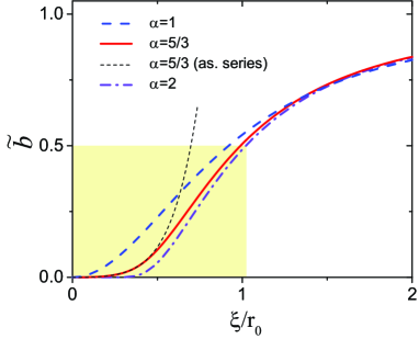
Figure 2: (Color online) Universal relative crosstalk amplitude $\tilde{b}$ versus $\xi/r_{0}$, for $\alpha=1$ [Eq. (21)], $\alpha=5/3$ [the universal function, Eqs. (22), and the asymptotic series, Eq. (68)], and $\alpha=2$ [Eq. (27)]. The shaded area highlights the parameter range $\tilde{b}\leq 1/2$ and $\xi/r_{0}\lesssim 1$, where the concurrence in Fig. 3 remains finite, due to Eq. (7).

III.3 Rescaled relative crosstalk amplitude and concurrence

In the limit $l_{0}\gg 1$, the expression for the phase correlation length given in Eq. (9) can be simplified by recalling the asymptotics of the sine, $\sin\left(\pi/2l_{0}\right)\sim\pi/2l_{0}$, and of the gamma-function Abramowitz and Stegun (1964):

$$\Gamma(l_{0}+x)\sim\sqrt{2\pi}e^{-l_{0}}l_{0}^{l_{0}+x-1/2}.$$ (19)

One obtains

$$\xi=\xi(l_{0})\sim\frac{\pi}{2\sqrt{2}}\frac{w_{0}}{\sqrt{l_{0}}},$$ (20)

which can be employed in Eqs. (13, 15, 18) to express the rescaled crosstalk in terms of $\xi/r_{0}$, yielding the sought-after universal behaviour. We find for $\alpha=1$,

$$\tilde{b}=\frac{\left(\gamma\xi/2r_{0}\right)^{2}}{\pi^{2}+\left(\gamma\xi/2r_{0}\right)^{2}};$$ (21)

for $\alpha=5/3$ (see B),

$$\tilde{b} =\sqrt{\frac{3}{5}}\frac{3^{3/5}}{(2\pi)^{3}}\frac{1}{\Gamma\left(\frac{8}{5}\right)}$$ (22)

$$\times\!\!\,{\rm Re}\,\!\!\left[G^{3,5}_{5,3}\left(\Biggl{.}\frac{-i\gamma^{3}5^{5}\xi^{5}}{\pi^{5}6^{3}r_{0}^{5}}\Biggr{|}\begin{array}[]{lllll}\frac{1}{5},&\frac{2}{5},&\frac{3}{5},&\frac{4}{5},&1\\ \frac{1}{5},&\frac{8}{15},&\frac{13}{15}&&\end{array}\right)\right]$$ (25)

$$\sim 0.29(\xi/r_{0})^{8/3},$$ (26)

with the bottom line of (26) valid in the limit $\xi/r_{0}\ll 1$, see Eqs. (16) and (20), and for $\alpha=2$,

$$\tilde{b}=\exp\left(-\frac{\pi^{2}r_{0}^{2}}{2\gamma\xi^{2}}\right).$$ (27)

It is easy to check that in all three cases, Eqs. (21 – 27), $\tilde{b}(0)=0$ and $\tilde{b}(\infty)=1$, where the latter value indicates the turbulence-induced saturation of the relative crosstalk amplitude. However, the behaviour of $\tilde{b}(\xi/r_{0})$ is rather distinct in the range $0<\xi/r_{0}\lesssim 1$ (see Fig. 2) for the three models of turbulence, what implies different forms of the entanglement decay (see Fig. 3).

Figure 3: (Color online) Universal decay of $C(\varrho)$ versus $\xi/r_{0}$, for $\alpha=1,5/3,2$, obtained from (7), with $\tilde{b}$ given, respectively, by Eqs. (21), (22) and (27). The thin dashed line that is nearly overlapping with the solid line represents the fitting function $g(\xi/r_{0})=\exp[-4.16(\xi/r_{0})^{3.24}]$ employed in Leonhard et al. (2015).

Figure 2 shows that the rescaled relative crosstalk amplitude $\tilde{b}$ is maximal for $\alpha=1$, and minimal for $\alpha=2$, in the range $0<\xi/r_{0}\lesssim 1$. Moreover, for $\alpha=2$, the amplitude $\tilde{b}$ remains vanishingly small for $\xi/r_{0}\lesssim 0.3$. This is a consequence of the exponential suppression of the crosstalk in the neighbourhood of $\xi/r_{0}=0$ [see Eq. (27)]. In contrast, for $\alpha=5/3$ and, especially, for $\alpha=1$, $\tilde{b}$ exhibits a power-law increase with $\xi/r_{0}$, by Eqs. (26, 21), and attains finite values in the interval $\xi/r_{0}\lesssim 0.3$. The behaviour of the universal functions $\tilde{b}$ at leading order in $\xi/r_{0}$ is summarized in Table 1 below, for the three models of turbulence considered here.

Table 1: Relative crosstalk amplitude $\tilde{b}$ in the limit $\xi/r_{0}\ll 1$, as a function of $\xi/r_{0}$, for the three models of turbulence here considered.

$\alpha=1$	$\alpha=5/3$	$\alpha=2$
(linear)	(Kolmogorov)	(quadratic)
$\tilde{b}\sim 1.20\left(\xi/r_{0}\right)^{2}$	$\tilde{b}\sim 0.29\left(\xi/r_{0}\right)^{8/3}$	$\tilde{b}=\exp\left(-\frac{\pi^{2}r_{0}^{2}}{13.76\,\xi^{2}}\right)$

Finally, inserting (21, 22, 27) into (7), we obtain the universal entanglement decay laws for the three considered models of turbulence which we present in Fig. 3. As anticipated, concurrence is most (least) robust against the rescaled turbulence strength for $\alpha=2$ ($\alpha=1$), with an intermediate behaviour for the Kolmogorov model. Apart from the three universal results here considered, we also plot the fitting function, $g(x)=\exp(-4.16\,x^{3.24})$ which was obtained for $\alpha=5/3$ in Leonhard et al. (2015). Although $g(x)$ is almost indistinguishable from the analytical result for finite values of $\xi/r_{0}$, our above discussion of the asymptotic behaviour of $\tilde{b}$ anticipates its limitations: Since $g(\xi/r_{0})$ vanishes exponentially as $\xi/r_{0}\to\infty$, Eq. (7) implies $\tilde{b}(\infty)=1/2$, in disagreement with the actual asymptotic limit $\tilde{b}(\infty)=1$.

IV Conclusion

We studied the entanglement evolution of photonic orbital angular momentum (OAM)bipartite qubit states in a weakly turbulent atmosphere, for three models of turbulence which are distinguished by the exponent $\alpha=1,5/3,2$ of the phase structure function $D_{\phi}(x)=\gamma\,(x/r_{0})^{\alpha}$. The entanglement evolution is entirely determined by the relative crosstalk amplitude $\tilde{b}$, such that an increase of $\tilde{b}$ entails a further loss of entanglement. $\tilde{b}$ is an $\alpha$-dependent, universal function of the ratio of the phase correlation length $\xi(l_{0})$ (of an OAM beam with azimuthal index $l_{0}$ and radial index $p=0$) to the atmospheric transverse correlation length $r_{0}$. Using asymptotic methods, we obtained explicit analytical expressions for $\tilde{b}(\xi(l_{0})/r_{0})$. In particular, for small $\xi(l_{0})/r_{0}\ll 1$, the relative crosstalk amplitude exhibits power-law dependencies $\sim(\xi(l_{0})/r_{0})^{2}$ and $\sim(\xi(l_{0})/r_{0})^{8/3}$ for $\alpha=1$ and $\alpha=5/3$, respectively, whereas it is exponentially suppressed for $\alpha=2$.

Our results shed new light on some earlier, related work Hamadou Ibrahim et al. (2013); Yan et al. (2016). In Hamadou Ibrahim et al. (2013), the concurrence decay of OAM bipartite qubit states (1) under Kolmogorov’s turbulence ($\alpha=5/3$) was studied numerically and experimentally for odd $l_{0}\leq 7$. The observed behaviour was then compared to analytical results Smith and Raymer (2006), obtained for $\alpha=2$. Good agreement was found between numerical simulations and analytical predictions Smith and Raymer (2006). However, a faster entanglement decay under Kolmogorov’s turbulence that is manifest in the simulations of Hamadou Ibrahim et al. (2013) for $l_{0}>1$ – in qualitative agreement with our present findings – was not discussed in Hamadou Ibrahim et al. (2013). Although this feature was reported in numerical simulations Yan et al. (2016), no analysis of the stronger robustness of entanglement for $\alpha=2$ was given. Curiously, although the experimental results of Hamadou Ibrahim et al. (2013) exhibit significant scatter of the data points, for $l_{0}=5$ and $l_{0}=7$ most of the points lie below the predicted evolution of concurrence for $\alpha=2$. We conjecture that this trend will prevail if the experiment is carried out using states with larger azimuthal indices. Furthermore, it is noteworthy that there is a close correspondence between the results of Hamadou Ibrahim et al. (2013); Yan et al. (2016), where the output state was projected onto $p=0$, and of our present findings, where the output state was averaged over the radial index $p$. It therefore appears that the dependence of the concurrence decay on $\alpha$ dominates its dependence on the radial structure of the output state – the latter being an open issue which should be addressed by future work.

Finally, our results suggest that the statistics of the wavefront distortions depends – via $D_{\phi}(x)$ – on the turbulence model. Therefore, another relevant future research topic is to identify the type of wavefront distortions resulting for distinct $\alpha$, especially for $\alpha=1$, wherein the entanglement decay is fastest. This information will potentially be useful when designing adaptive optics systems aimed at entanglement protection of twisted photons under weak to moderate turbulence Leonhard et al. (2018).

Appendix A Derivation of equation (3)

Here, closely following Leonhard (2014), we present a step by step derivation of the map operator (3) corresponding to a single phase screen. As mentioned above in section II, our model neglects scintillations and beam diffraction, and is thus limited to relatively short (of about $1$ km) propagation distances, for each photon. For convenience, we apply a single phase screen to a Laguere-Gaussian (LG) beam at $z=0$. Since the propagation through vacuum does not affect the beam’s structure, we drop the $z$-dependence in all subsequent expressions, while including the propagation distance $L$ in the definition of the Fried parameter (6).

Let us denote by $|p,l\rangle$ a single photon state populating the LG mode ${\rm LG}_{p,l}(r,\theta)$, i.e.,

$$\langle r,\theta|p,l\rangle:={\rm LG}_{p,l}(r,\theta).$$ (28)

Any pure state $|\Psi_{0}\rangle$ can be expanded in terms of OAM basis states $|p,l\rangle$:

$$|\Psi_{0}\rangle=\sum_{p,l}c_{p,l}|p,l\rangle,$$ (29)

with $c_{p,l}$ given by the overlap integrals

$$c_{p,l}:=\frac{1}{2\pi}\int_{0}^{\infty}\int_{0}^{2\pi}{\rm LG}^{*}_{p,l}(r,\theta)\Psi_{0}(r,\theta)r\mathrm{d}r\mathrm{d}\theta,$$ (30)

where $\Psi_{0}(r,\theta):=\langle r,\theta|\Psi_{0}\rangle$ is the mode function of the initial state.

The application of a phase screen to $|\Psi_{0}\rangle$ amounts to adding a random position-dependent phase $\phi(r,\theta)$ to the photon’s wavefront:

$$|\Psi_{0}\rangle\rightarrow|\tilde{\Psi}\rangle=|\Psi_{0}\rangle e^{i\phi(r,\theta)}.$$ (31)

Therefore, the expansion coefficients of $|\tilde{\Psi}\rangle$ in the OAM basis read

$$\tilde{c}_{p,l}:=\frac{1}{2\pi}\int_{0}^{\infty}\int_{0}^{2\pi}{\rm LG}^{*}_{p,l}(r,\theta)e^{i\phi(r,\theta)}\Psi_{0}(r,\theta)r\mathrm{d}r\mathrm{d}\theta.$$ (32)

Due to the phase factor $e^{i\phi(r,\theta)}$, the output state $|\tilde{\Psi}\rangle$ has an overlap with initially unpopulated OAM modes. In other words, phase aberrations lead to crosstalk among different OAM modes.

Performing an ensemble average over phase screens with a given Fried parameter $r_{0}$, we obtain a mixed output state,

$$\varrho :=\big{\langle}|\tilde{\Psi}\rangle\langle\tilde{\Psi}|\big{\rangle}=\sum_{p_{1},l_{1},p_{2},l_{2}}\langle\tilde{c}_{p_{1},l_{1}}\tilde{c}_{p_{2},l_{2}}^{*}\rangle|p_{1},l_{1}\rangle\langle p_{2},l_{2}|$$

$$=\sum_{p_{1},l_{1},p_{2},l_{2}}\varrho_{p_{1},l_{1},p_{2},l_{2}}|p_{1},l_{1}\rangle\langle p_{2},l_{2}|,$$ (33)

with the matrix elements of the output state

$$\varrho_{p_{1},l_{1},p_{2},l_{2}} =\frac{1}{4\pi^{2}}\int_{0}^{\infty}\int_{0}^{2\pi}\int_{0}^{\infty}\int_{0}^{2\pi}r\mathrm{d}r\mathrm{d}\theta\,\,r^{\prime}\mathrm{d}r^{\prime}\mathrm{d}\theta^{\prime}$$

$$\times{\rm LG}^{*}_{p_{1},l_{1}}(r,\theta){\rm LG}_{p_{2},l_{2}}(r^{\prime},\theta^{\prime})\Psi_{0}(r,\theta)\Psi_{0}^{*}(r^{\prime},\theta^{\prime})$$

$$\times\Big{\langle}\exp[i\phi(r,\theta)-i\phi(r^{\prime},\theta^{\prime})]\Big{\rangle}.$$ (34)

Within the Kolmogorov turbulence model, the ensemble average in (34) yields the result Paterson (2005)

$$\Big{\langle}\exp[i\phi(r,\theta)-i\phi(r^{\prime},\theta^{\prime})]\Big{\rangle}=\exp\Big{[}-\frac{1}{2}D_{\phi}(|\vec{r}-\vec{r}\mkern 2.0mu\vphantom{r}^{\prime}|)\Big{]},$$ (35)

where $D_{\phi}(|\vec{r}-\vec{r}\mkern 2.0mu\vphantom{r}^{\prime}|)$ is the phase structure function given by Fried (1965),

$$D_{\phi}(|\vec{r}-\vec{r}\mkern 2.0mu\vphantom{r}^{\prime}|)=6.88\left(\frac{|\vec{r}-\vec{r}\mkern 2.0mu\vphantom{r}^{\prime}|}{r_{0}}\right)^{5/3}.$$ (36)

We note that (36) coincides with (5) for $\alpha=5/3$ and $x=|\vec{r}-\vec{r}\mkern 2.0mu\vphantom{r}^{\prime}|$.

From equations (28), (29), (33)-(35), the effect of the ensemble-averaged phase aberrations on any pure initial OAM state can be represented by the map operator $\Lambda$ as follows:

$$\varrho_{p_{1},l_{1},p_{2},l_{2}}=\sum_{p_{0},l_{0},p_{0}^{\prime},l_{0}^{\prime}}\Lambda_{p_{1},l_{1},p_{2},l_{2}}^{p_{0},l_{0},p_{0}^{\prime},l_{0}^{\prime}}\,c_{p_{0},l_{0}}c^{*}_{p_{0}^{\prime},l_{0}^{\prime}},$$ (37)

where

$$\Lambda_{p_{1},l_{1},p_{2},l_{2}}^{p_{0},l_{0},p_{0}^{\prime},l_{0}^{\prime}} =\frac{1}{4\pi^{2}}\int_{0}^{\infty}\int_{0}^{2\pi}\int_{0}^{\infty}\int_{0}^{2\pi}r\mathrm{d}r\mathrm{d}\theta\,\,r^{\prime}\mathrm{d}r^{\prime}\mathrm{d}\theta^{\prime}$$

$$\times{\rm LG}^{*}_{p_{1},l_{1}}(r,\theta){\rm LG}_{p_{2},l_{2}}(r^{\prime},\theta^{\prime})$$

$$\times{\rm LG}_{p_{0},l_{0}}(r,\theta){\rm LG}_{p_{0}^{\prime},l_{0}^{\prime}}^{*}(r^{\prime},\theta^{\prime})$$

$$\times\exp\left[-\frac{1}{2}D_{\phi}\left(|\vec{r}-\vec{r}\mkern 2.0mu\vphantom{r}^{\prime}|\right)\right].$$ (38)

By factorizing the mode functions ${\rm LG}_{p,l}(r,\theta)=R_{p,l}(r)e^{il\theta}$ into products of their radial part $R_{p,l}(r)$ and a complex phase $e^{il\theta}$ Siegman (1986), we obtain

$$\Lambda_{p_{1},l_{1},p_{2},l_{2}}^{p_{0},l_{0},p_{0}^{\prime},l_{0}^{\prime}} =\frac{1}{4\pi^{2}}\int_{0}^{\infty}\int_{0}^{2\pi}\int_{0}^{\infty}\int_{0}^{2\pi}R^{*}_{p_{1},l_{1}}(r)R_{p_{2},l_{2}}(r^{\prime})R_{p_{0},l_{0}}(r)R_{p_{0}^{\prime},l_{0}^{\prime}}^{*}(r^{\prime})$$

$$\times e^{-il_{1}\theta+il_{2}\theta^{\prime}+il_{0}\theta-il_{0}^{\prime}\theta^{\prime}}\exp\left[-\frac{1}{2}D_{\phi}\left(|\vec{r}-\vec{r}\mkern 2.0mu\vphantom{r}^{\prime}|\right)\right]r\mathrm{d}r\mathrm{d}\theta\,\,r^{\prime}\mathrm{d}r^{\prime}\mathrm{d}\theta^{\prime}.$$ (39)

To simplify this expression, we introduce new angular variables $\vartheta$ and $\Theta$,

$$\vartheta:=\theta-\theta^{\prime},\quad\Theta:=\frac{\theta+\theta^{\prime}}{2},$$ (40)

and take the integral over the angle $\Theta$,

$$\int_{0}^{2\pi}e^{i(l_{0}-l_{0}^{\prime}-l_{1}+l_{2})\vartheta}\mathrm{d}\Theta=2\pi\delta_{l_{0}-l_{0}^{\prime},l_{1}-l_{2}}.$$ (41)

Next, when tracing the output state over the radial quantum number $p$ (see section II),

$$\varrho_{l_{1},l_{2}}=\sum_{p=0}^{\infty}\varrho_{p,l_{1},p,l_{2}},$$ (42)

we focus on the special case $|l_{1}|=|l_{2}|=:l$. Therein, the symmetry holds,

$$R_{p,l}(r)=R_{p,-l}(r),$$ (43)

which follows from the general expression for LG functions Siegman (1986). Finally, using the commutativity of the summation over $p$ and the integration over $r^{\prime}$, we can employ the completeness relation Abramowitz and Stegun (1964):

$$\sum_{p=0}^{\infty}R_{p,l}(r)R_{p,l}^{*}(r^{\prime})=\frac{1}{r}\delta(r-r^{\prime}),$$ (44)

to perform the integration over $r^{\prime}$ in (39) and to arrive at the following expression for the matrix elements of the turbulence map:

$$\Lambda_{l,\pm l}^{p_{0},l_{0},p_{0}^{\prime},l_{0}^{\prime}}=\frac{1}{2\pi}\delta_{l_{0}-l_{0}^{\prime},l\pm l}\int_{0}^{\infty}\int_{0}^{2\pi}R_{p_{0},l_{0}}(r)R_{p_{0}^{\prime},l_{0}^{\prime}}^{*}(r)e^{-i\frac{\vartheta}{2}[(l\pm l)-(l_{0}+l_{0}^{\prime})]}\exp\left\{-\frac{1}{2}D_{\phi}\left[2r\sin\left(\frac{\vartheta}{2}\right)\right]\right\}r\mathrm{d}r\,\mathrm{d}\vartheta,$$ (45)

which coincides with (3) for $p_{0}=p_{0}^{\prime}=0$. As we take the above steps, the argument $|\vec{r}-\vec{r}\mkern 2.0mu\vphantom{r}^{\prime}|$ of the phase structure function $D_{\phi}(|\vec{r}-\vec{r}\mkern 2.0mu\vphantom{r}^{\prime}|)$ undergoes the following transformations:

$$|\vec{r}-\vec{r}\mkern 2.0mu\vphantom{r}^{\prime}| =\sqrt{r^{2}+r^{\prime 2}-2rr^{\prime}\cos(\theta-\theta^{\prime})}$$ (46)

$$\stackrel{{\scriptstyle\eqref{angles}}}{{=}}\sqrt{r^{2}+r^{\prime 2}-2rr^{\prime}\cos(\vartheta)}$$

$$\stackrel{{\scriptstyle\eqref{eq:traceout}}}{{=}}\sqrt{2r^{2}[1-\cos(\vartheta)]}$$

$$=2r|\sin(\vartheta/2)|=2r\sin(\vartheta/2),$$ (47)

where the last equality follows, since $\sin(x)\geq 0$ if $0\leq x\leq\pi$.

Appendix B Asymptotic evaluation of equation (3)

Equation (3) can be rewritten in the form:

$$\Lambda_{l_{1},l_{1}}^{l_{0},l_{0}} =\frac{2^{l_{0}+1}}{\pi l_{0}!}\int_{0}^{\infty}\int_{0}^{2\pi}\mathrm{d}\rho\mathrm{d}\vartheta e^{i\vartheta(l_{1}-l_{0})}$$

$$\times\exp\left[(2l_{0}+1)\ln(\rho)-2\rho^{2}-d(\vartheta)\rho^{\alpha}\right],$$ (48)

where $\rho\equiv r/w_{0}$, $1\leq\alpha\leq 2$, and

$$d(\vartheta)=2^{\alpha-1}\gamma\left(\frac{w_{0}}{r_{0}}\right)^{\alpha}\sin^{\alpha}\left(\frac{\vartheta}{2}\right).$$ (49)

We first note that, for arbitrary $l_{0}$, $l_{1}$, $\alpha$, $w_{0}/r_{0}$, and for any fixed $\rho\geq 0$, the integral over $\vartheta$ in Eq. (48) is real. The corresponding integrand, $\exp\{-d(\vartheta)\rho^{\alpha}+i\vartheta(l_{1}-l_{0})\}$, attains maximum values at the end points of the integration region and is symmetric under reflection with respect to the $\vartheta=\pi$ axis. Therefore, when evaluating the integral over $\vartheta$, we can consider only the values $\vartheta\ll 1$. We use this consideration in our subsequent analysis of the integral over $\rho$ in Eq. (48), which is a Laplace integral Erdélyi (1956),

$$\int_{0}^{\infty}\mathrm{d}\rho\exp[\lambda f(\rho)],$$ (50)

with

$$f(\rho)=\ln\rho-\frac{2\rho^{2}-d(\vartheta)\rho^{\alpha}}{2l_{0}+1},$$ (51)

and $\lambda=2l_{0}+1$. For $l_{0}\gg 1$, the asymptotics of the integral (50) can be evaluated using the method of steepest descent Carrier et al. (2005); Erdélyi (1956), according to which the main contribution to (50) comes from the neighborhood of the saddle points of the exponential $f(\rho)$. The function $f(\rho)$ has a non-degenerate saddle point at

$$\rho_{m}\approx\sqrt{l_{0}/2},$$ (52)

where we neglected the term proportional to $d(\vartheta)$ in (51) above. Inserting the expansion $f(\rho)\approx f(\rho_{m})+f^{\prime\prime}(\rho_{m})(\rho-\rho_{m})^{2}$ into (48), extending the lower limit of the integral over $\rho$ to $-\infty$, and evaluating the resulting Gaussian integral, we arrive at the intermediate expression

$$\Lambda_{l_{1},l_{1}}^{l_{0},l_{0}}\approx\frac{1}{\pi}{\rm Re}\left[\int_{0}^{\pi}\mathrm{d}\vartheta\exp\{-A\vartheta^{\alpha}+i\vartheta(l_{1}-l_{0})\}\right],$$ (53)

where

$$A=\gamma 2^{-\alpha/2-1}\,l_{0}^{\alpha/2}\,(w_{0}/r_{0})^{\alpha}.$$ (54)

For $l_{1}=l_{0}$ and $l_{1}=-l_{0}$, Eq. (53) yields the amplitudes $a$ and $b$, respectively. For the survival amplitude $a$, one immediately obtains,

$$a\approx\frac{1}{\pi}A^{-1/\alpha}\Gamma\left(1+\frac{1}{\alpha}\right).$$ (55)

Since the main contribution to the crosstalk amplitude,

$$b\approx\frac{1}{\pi}{\rm Re}\left[\int_{0}^{\pi}\mathrm{d}\vartheta\exp(-A\vartheta^{\alpha}-2il_{0}\vartheta)\right],$$ (56)

originates from $\vartheta\ll 1$, we can replace the upper integration limit by infinity, to obtain

$$b\approx\frac{1}{\pi}{\rm Re}\left[\int_{0}^{\infty}\mathrm{d}\vartheta\exp(-A\vartheta^{\alpha}-2il_{0}\vartheta)\right]=:\frac{1}{\pi}{\rm Re}[J].$$ (57)

For $\alpha=1$ and $\alpha=2$, the oscillatory integral $J$ in Eq. (57) reduces to the Fourier transform of, respectively, an exponential and a Gaussian function. The parameter $b$ can be then easily calculated to yield Eqs. (13) and (18) for $\alpha=1$ and $\alpha=2$, respectively. For $\alpha=5/3$, Eq. (57) can be transformed to a tabulated integral, by a rotation of the real semi-axis by an angle $\beta$ into the complex plane Carrier et al. (2005). Then the integral $J$ transforms into

$$J=e^{i\beta}\int_{0}^{\infty}\mathrm{d}x\exp(-qx^{\alpha}-sx),$$ (58)

where $q=A\exp(i\alpha\beta)$ and $s=2il_{0}\exp(i\beta)$. The integral on the right hand side of Eq. (58) converges if ${\rm Re}(q)>0$, ${\rm Re}(s)>0$. To ensure that both inequalities are satisfied for $\alpha=5/3$ and for convenience, we choose $\beta=-\pi/5$. The exact value of Eq. (58) can be found in Prudnikov et al. (1992); it is expressed in terms of the Meijer G-function Bateman (1953), see Eq. (15b). We mention that the same method can also be used to find $b$ for other $\alpha=l/k$, where $l,k$ are positive integers, and in particular for $\alpha=1$ and $\alpha=2$. In the latter case, the Meijer G-function simplifies to the expressions for $b$ given by Eqs. (13) and (18), respectively.

The relative crosstalk amplitude, derived directly from Eqs. (15a) and (15b), reads

$$\tilde{b} =\!\sqrt{\frac{3}{5}}\frac{3^{\frac{3}{5}}}{(2\pi)^{3}}\frac{1}{\Gamma\left(\frac{8}{5}\right)}$$

$$\,{\rm Re}\,\!\!\left[z^{\frac{1}{5}}G^{3,5}_{5,3}\left(\!\Biggl{.}z\Biggr{|}\begin{array}[]{lllll}0,&\!\frac{1}{5},&\!\frac{2}{5},&\!\frac{3}{5},&\!\frac{4}{5}\\ 0,&\!\frac{1}{3},&\!\frac{2}{3}&&\end{array}\right)\!\right],$$ (61)

where

$$z=-i\frac{5^{5}t^{5}\gamma^{3}}{3^{3}2^{21/2}l_{0}^{5/2}}.$$

To show that $\tilde{b}$ is a function of the sole parameter $\xi/r_{0}$, we use the identity Bateman (1953)

$$z^{\sigma}G^{m,n}_{p,q}\left(\Biggl{.}z\Biggr{|}\begin{array}[]{l}a_{r}\\ b_{r^{\prime}}\end{array}\right)=G^{m,n}_{p,q}\left(\Biggl{.}z\Biggr{|}\begin{array}[]{l}a_{r}+\sigma\\ b_{r^{\prime}}+\sigma\end{array}\right),$$ (62)

where $a_{r}$ ($b_{r^{\prime}}$) represent the upper (lower) vectors of the Meijer G-function (e.g., in Eq. (61), $a_{r}=\{0,1/5,2/5,3/5,4/5\}$) and the summation in the right-hand side of (62) is to be understood element-wise. Applying the identity (62) to Eq. (61), we arrive at the result

$$\tilde{b} =\sqrt{\frac{3}{5}}\frac{3^{3/5}}{(2\pi)^{3}}\frac{1}{\Gamma\left(\frac{8}{5}\right)}$$ (63)

$$\times\!\!\,{\rm Re}\,\!\!\left[G^{3,5}_{5,3}\left(\Biggl{.}\frac{-i\gamma^{3}5^{5}\xi^{5}}{\pi^{5}6^{3}r_{0}^{5}}\Biggr{|}\begin{array}[]{lllll}\frac{1}{5},&\frac{2}{5},&\frac{3}{5},&\frac{4}{5},&1\\ \frac{1}{5},&\frac{8}{15},&\frac{13}{15}&&\end{array}\right)\right].$$ (66)

Whereas the limiting values $0$ and $1$ of $\tilde{b}$ for $\xi\to 0$ and $\xi\to\infty$, respectively, can be directly computed from Eq. (63), the asymptotics of $\tilde{b}$ for $\xi/r_{0}\ll 1$ (or $w_{0}/r_{0}\sqrt{l_{0}}\ll 1$) is easier to deduce directly from Eqs. (55), (57) and (58). It follows from (55) and (57) that $\tilde{b}=\,{\rm Re}\,[J]/(\pi a)$. Using Watson’s lemma Carrier et al. (2005), we obtain the asymptotic series expansion of the integral (58):

$$J=e^{i\beta}\frac{1}{s}\sum_{n=0}^{\infty}\frac{(-1)^{n}}{n!}\left(\frac{q}{s^{\alpha}}\right)^{n}\Gamma(1+n\alpha).$$ (67)

Substituting the values $\alpha=5/3$, $\beta=-\pi/5$, $s=2il_{0}\,e^{-i\pi/5}$, $q=6.88\times 2^{-11/6}\,t^{5/3}\,l_{0}^{5/6}e^{-i\pi/3}$ and $a=\pi^{-1}q^{-3/5}e^{-i\pi/5}\Gamma(1+3/5)$ into the ratio $\tilde{b}=\,{\rm Re}\,[J]/(\pi a)$, after some simple algebra we obtain

$$\tilde{b} \approx 0.380\!\left(\!\frac{t^{2}}{l_{0}}\!\right)^{\!\!\frac{4}{3}}\!\!\!\!+\!1.231\!\left(\!\frac{t^{2}}{l_{0}}\!\right)^{\!\!\frac{13}{6}}\!\!\!\!\!\!+\!3.735\!\left(\!\frac{t^{2}}{l_{0}}\!\right)^{\!\!3}\!\!\!+\!O\!\!\left[\left(\!\frac{t^{2}}{l_{0}}\!\right)^{\!\frac{23}{6}}\right]$$

$$=0.287\!\left(\!\frac{\xi}{r_{0}}\!\right)^{\!\!\frac{8}{3}}\!\!\!+\!0.781\!\left(\!\frac{\xi}{r_{0}}\!\right)^{\!\!\frac{13}{3}}\!\!\!\!\!\!+\!1.989\!\left(\!\frac{\xi}{r_{0}}\!\right)^{\!\!6}\!\!\!+\!O\!\left[\left(\!\frac{\xi}{r_{0}}\!\right)^{\!\frac{23}{3}}\right],$$ (68)

where the top line reproduces (16) and the bottom line is used in Fig. 2. Note an increase of the subsequent expansion coefficients in (68). Starting from some $n$, which value depends on $t$ and $l_{0}$, these coefficients dominate the decreasing magnitude of $(t^{2}/l_{0})^{(4+5n)/3}$ in the asymptotic expansion of $\tilde{b}$ (for $t=5.0$ and $l_{0}=150$, this occurs at $n=7$). This behaviour indicates divergence of Eq. (67) – the common feature of asymptotic series Dingle (1973). However, a finite number of terms in Eq. (67) yields an accurate asymptotic description of $\tilde{b}$. We empirically established that the first three terms of the series (68) provide the best overlap with the exact behaviour of $\tilde{b}$ at $l_{0}\gtrsim 150$ and $0.1\leq t\leq 5.0$ (i.e., for $0.0091\leq\xi/r_{0}\leq 0.45$), see Figs.1 and 2.

References

- Allen et al. (1992) L. Allen, M. W. Beijersbergen, R. J. C. Spreeuw, and J. P. Woerdman, Phys. Rev. A 45, 8185 (1992).
- Molina-Terriza et al. (2007) G. Molina-Terriza, J. P. Torres, and L. Torner, Nat. Phys. 3, 305 (2007).
- Franke-Arnold et al. (2008) S. Franke-Arnold, L. Allen, and M. Padgett, Las. & Photon. Rev. 2, 299 (2008).
- Gibson et al. (2004) G. Gibson, J. Courtial, M. Padgett, M. Vasnetsov, V. Pas’ko, S. Barnett, and S. Franke-Arnold, Opt. Express 12, 5448 (2004).
- Barreiro et al. (2008) J. T. Barreiro, T.-C. Wei, and P. G. Kwiat, Nat. Phys. 4, 282 (2008).
- Bechmann-Pasquinucci and Peres (2000) H. Bechmann-Pasquinucci and A. Peres, Phys. Rev. Lett. 85, 3313 (2000).
- Bourennane et al. (2001) M. Bourennane, A. Karlsson, and G. Björk, Phys. Rev. A 64, 012306 (2001).
- Tatarskii (1961) V. I. Tatarskii, Wave Propagation in a Turbulent Medium (McGraw-Hill, New York, 1961).
- Vallone et al. (2014) G. Vallone, V. D’Ambrosio, A. Sponselli, S. Slussarenko, L. Marrucci, F. Sciarrino, and P. Villoresi, Phys. Rev. Lett. 113, 060503 (2014).
- Sit et al. (2017) A. Sit, F. Bouchard, R. Fickler, J. Gagnon-Bischoff, H. Larocque, K. Heshami, D. Elser, C. Peuntinger, K. Günthner, B. Heim, C. Marquardt, G. Leuchs, R. W. Boyd, and E. Karimi, Optica 4, 1006 (2017).
- Krenn et al. (2015) M. Krenn, J. Handsteiner, M. Fink, R. Fickler, and A. Zeilinger, Proc. Natl. Acad. Sci. USA 112, 14197 (2015).
- Krenn et al. (2016) M. Krenn, J. Handsteiner, M. Fink, R. Fickler, R. Ursin, M. Malik, and A. Zeilinger, Proc. Natl. Acad. Sci. USA 113, 13648 (2016).
- Ekert (1991) A. K. Ekert, Phys. Rev. Lett. 67, 661 (1991).
- Mintert et al. (2005) F. Mintert, A. R. Carvalho, M. Kuś, and A. Buchleitner, Phys. Rep. 415, 207 (2005).
- Horodecki et al. (2009) R. Horodecki, P. Horodecki, M. Horodecki, and K. Horodecki, Rev. Mod. Phys. 81, 865 (2009).
- Mair et al. (2001) A. Mair, A. Vaziri, G. Weihs, and A. Zeilinger, Nature 412, 313 (2001).
- Fickler et al. (2012) R. Fickler, R. Lapkiewicz, W. N. Plick, M. Krenn, C. Schaeff, S. Ramelow, and A. Zeilinger, Science 338, 640 (2012).
- van Exter et al. (2012) M. P. van Exter, E. R. Eliel, and J. P. Woerdman, in The Angular Momentum of Light, edited by D. L. Andrews and M. Babiker (Cambridge University Press, Cambridge, UK, 2012).
- Pors et al. (2011) B.-J. Pors, C. H. Monken, E. R. Eliel, and J. P. Woerdman, Opt. Express 19, 6671 (2011).
- Hamadou Ibrahim et al. (2013) A. Hamadou Ibrahim, F. S. Roux, M. McLaren, T. Konrad, and A. Forbes, Phys. Rev. A 88, 012312 (2013).
- Zhang et al. (2016) Y. Zhang, S. Prabhakar, A. H. Ibrahim, F. S. Roux, A. Forbes, and T. Konrad, Phys. Rev. A 94, 032310 (2016).
- Goyal et al. (2016) S. K. Goyal, A. H. Ibrahim, F. S. Roux, T. Konrad, and A. Forbes, J. Opt. 18, 064002 (2016).
- Ndagano et al. (2017) B. Ndagano, B. Perez-Garcia, F. S. Roux, M. McLaren, C. Rosales-Guzman, Y. Zhang, O. Mouane, R. I. Hernandez-Aranda, T. Konrad, and A. Forbes, Nat. Phys. 13, 397 (2017).
- Gopaul and Andrews (2007) C. Gopaul and R. Andrews, New J. Phys. 9, 94 (2007).
- Sheng et al. (2012) X. Sheng, Y. Zhang, F. Zhao, L. Zhang, and Y. Zhu, Opt. Lett. 37, 2607 (2012).
- Roux (2011) F. S. Roux, Phys. Rev. A 83, 053822 (2011).
- Ibrahim et al. (2014) A. H. Ibrahim, F. S. Roux, and T. Konrad, Phys. Rev. A 90, 052115 (2014).
- Roux et al. (2015) F. S. Roux, T. Wellens, and V. N. Shatokhin, Phys. Rev. A 92, 012326 (2015).
- Roux (2017) F. S. Roux, Phys. Rev. A 95, 023809 (2017).
- Smith and Raymer (2006) B. J. Smith and M. G. Raymer, Phys. Rev. A 74, 062104 (2006).
- Leonhard et al. (2015) N. D. Leonhard, V. N. Shatokhin, and A. Buchleitner, Phys. Rev. A 91, 012345 (2015).
- Wootters (1998) W. K. Wootters, Phys. Rev. Lett. 80, 2245 (1998).
- Andrews and Phillips (2005) L. C. Andrews and R. L. Phillips, Laser Beam Propagation through Random Media, second ed. (SPIE Press, Bellingham, 2005).
- Buckley (1975) R. Buckley, J. Atmos. Terr. Phys. 37, 1431 (1975).
- Kropf et al. (2016) C. M. Kropf, C. Gneiting, and A. Buchleitner, Phys. Rev. X 6, 031023 (2016).
- Paterson (2004) C. Paterson, Proc. SPIE 5572, 187 (2004).
- Bertlmann et al. (2003) R. A. Bertlmann, K. Durstberger, and B. C. Hiesmayr, Phys. Rev. A 68, 012111 (2003).
- Fried (1965) D. L. Fried, J. Opt. Soc. Am. 55, 1427 (1965).
- Fried (1966) D. L. Fried, J. Opt. Soc. Am. 56, 1372 (1966).
- Leader (1978) J. C. Leader, J. Opt. Soc. Am. 68, 175 (1978).
- Chandrasekaran and Shapiro (2014) N. Chandrasekaran and J. H. Shapiro, J. Lightwave Technol. 32, 1075 (2014).
- Carrier et al. (2005) G. F. Carrier, M. Krook, and C. E. Pearson, Functions of a Complex Variable: Theory and Technique, Vol. 49 (SIAM, New York, 2005).
- Prudnikov et al. (1992) A. P. Prudnikov, Y. A. Brychkov, and O. Marichev, Integrals and Series: Direct Laplace Transforms, Vol. 4 (Gordon and Breach Science Publishers, New York, 1992).
- Bateman (1953) H. Bateman, Higher Transcendental Functions, Vol. I (McGraw-Hill Book Co. Inc., New York, 1953).
- Abramowitz and Stegun (1964) M. Abramowitz and I. A. Stegun, eds., Handbook of Mathematical Functions with Formulas, Vol. 55 (National Bureau of Standards, Washington, D.C., 1964).
- Dingle (1973) R. B. Dingle, Asymptotic Expansions: Their Derivation and Interpretation (Academic Press, London, 1973).
- Prudnikov et al. (1990) A. P. Prudnikov, Y. A. Brychkov, and O. Marichev, Integrals and Series: Special functions, Vol. 2 (Gordon and Breach Science Publishers, New York, 1990).
- Yan et al. (2016) X. Yan, P. F. Zhang, J. H. Zhang, H. Q. Chun, and C. Y. Fan, J. Opt. Soc. Am. A 33, 1831 (2016).
- Leonhard et al. (2018) N. Leonhard, G. Sorelli, V. N. Shatokhin, C. Reinlein, and A. Buchleitner, Phys. Rev. A 97, 012321 (2018).
- Leonhard (2014) N. Leonhard, “Propagation of orbital angular momentum photons through atmospheric turbulence,” Diploma thesis (Albert-Ludwigs University of Freiburg) (2014).
- Paterson (2005) C. Paterson, Phys. Rev. Lett. 94, 153901 (2005).
- Siegman (1986) A. Siegman, Lasers (University Science Books, Mill Valey, California, 1986).
- Erdélyi (1956) A. Erdélyi, Asymptotic expansions (Dover Publications, Inc., New York, 1956).