A New, Deep JVLA Radio Survey of M33

Abstract

We have performed new 1.4 GHz and 5 GHz observations of the Local Group galaxy M33 with the Jansky Very Large Array. Our survey has a limiting sensitivity of 20 $\mu$Jy ($4\sigma$) and a resolution of 5.9″ (FWHM), corresponding to a spatial resolution of 24 pc at 817 kpc. Using a new multi-resolution algorithm, we have created a catalog of 2875 sources, including 675 with well-determined spectral indices. We detect sources at the position of 319 of the X-ray sources in the Tüllmann et al.  (2011) Chandra survey of M33, the majority of which are likely to be background galaxies. The radio source coincident with M33 X-8, the nuclear source, appears to be extended. Along with numerous H II regions or portions of H II region complexes, we detect 155 of the 217 optical supernova remnants included in the lists of Long et al. (2010) and Lee & Lee (2014), making this by far the largest sample of remnants at known distances with multiwavelength coverage. The remnants show a large dispersion in the ratio of radio to X-ray luminosity at a given diameter, a result that challenges the current generation of models for synchrotron radiation evolution in supernova remnants.

Accepted for publication in the Astrophysical Journal

1 Introduction

Supernova remnants (SNRs), the long-lasting products of supernovae (SNe), are the working surfaces at which SNe chemically enrich, and deposit kinetic energy into, the surrounding circumstellar and interstellar medium. In extreme cases, the collective action of many SNe can even drive outflows in starburst galaxies. SNRs are also almost certainly the dominant source of cosmic rays in a galaxy. As such, SNRs are central to our understanding of the life cycle of stars and the evolution of galaxies, as well as for the composition and dynamics of the interstellar and intergalactic media.

Observations of external galaxies offer the best way to study the class properties of SNRs, since all of the SNRs are effectively at the same distance and problems associated with dust extinction in the plane of our Galaxy are minimized. For example, only about 30% of the 294 Galactic SNRs in the catalog by Green (2014) have been detected at optical wavelengths and just 40% have been detected in X-rays, primarily due to limitations imposed by line-of-sight dust and gas extinction. Also, the distances to individual Galactic SNRs are often highly uncertain. It has thus been difficult to systematically study unbiased samples of Galactic SNRs at all wavelengths.

Most Galactic SNRs were first discovered as spatially extended, non-thermal radio sources, and the first studies of the class properties of SNRs were largely based on radio observations alone (see, e.g., Green 2009 and references therein). In contrast, most extragalactic SNRs have been identified from deep optical interference filter imagery, where the ratio of [S II] $\lambda\lambda$ 6717,6731 to H$\alpha$ provides an effective discriminant between H II regions ([S II]:H$\alpha$ $\sim$ 0.1) and SNRs ([S II]:H$\alpha$ $\gtrsim 0.4$), at least for the brighter objects (Long et al., 2018). Except in the Magellanic Clouds, radio and X-ray instrumentation has not hitherto had the appropriate combination of spatial resolution and sensitivity to detect large numbers of extragalactic SNRs, let alone discover new ones.

M33 is arguably the best external galaxy in which to study SNRs because it is nearby ($817\pm 58$ kpc, so 1″ = 4 pc, Freedman et al., 2001), relatively face on ($i=56\pm 1\arcdeg$, Zaritsky et al., 1989), and has relatively low Galactic foreground absorption ($N_{\mathrm{H}}=\mbox{\rm$6\times 10^{20}\rm\>cm^{-2}$}$, Dickey & Lockman, 1990; Stark et al., 1992). While the Large and Small Magellanic Clouds are both $\sim 15$ times closer than M33 (50 kpc and 60 kpc, respectively, Pietrzyński et al., 2013; Hilditch et al., 2005) and have similarly low foreground absorption, the SNR samples in the LMC and SMC are far more limited than that in M33. Furthermore, M33 has been well-studied across the electromagnetic spectrum, providing a wealth of supporting information.

The first three optical SNR candidates in M33 were identified forty years ago by D’Odorico et al. (1978), and the numbers have grown significantly since then, especially after CCDs made interference filter imaging searches for SNRs more efficient (D’Odorico et al., 1980; Long et al., 1990; Gordon et al., 1998; Long et al., 2010). The two most recent optical surveys were carried out using data originally obtained as part of the Local Group Galaxy Survey (LGGS, Massey et al., 2006, 2007). Surveys by Long et al. (2010, hereafter L10) and by Lee & Lee (2014a, hereafter LL14) found 137 and 199 optical SNRs or candidates, respectively. After overlaps between the two lists are eliminated, there are 217 unique SNR candidates in M33 (Long et al., 2018, hereafter L18).

The original selection of these nebulae as candidates was made on the basis of elevated [S II]:H$\alpha$ ratios in emission line imagery, but imaging surveys have limitations due to the potential for contamination of the H$\alpha$ filter image by varying amounts of [N II] $\lambda\lambda$6548,6584 emission. Most of the M33 SNRs have now been shown to have bona fide high [S II]:H$\alpha$ ratios via optical spectroscopy, which resolves the [N II]–H$\alpha$ complex and allows a clean H$\alpha$ measurement (L18). Finally, of the 217 SNR candidate nebulae, 112 have been detected in X-rays, either using Chandra (L10) and/or XMM-Newton (Garofali et al., 2017).

Early radio observations of M33 were limited by the resolution and sensitivity available from single-dish telescopes (Dennison et al., 1975), but with the advent of powerful interferometers it became possible to detect individual objects within the galaxy. D’Odorico et al. (1982) were the first to detect M33 optical SNRs at radio wavelengths; they concluded that the luminosities of SNRs in M33 were similar to those in the Galaxy. A more detailed study of the radio SNRs in M33 was carried out by Gordon et al. (1999, hereafter G99) using a combination of the Westerbork Synthesis Radio Telescope and the (original) Very Large Array at 5 GHz and 1.4 GHz. They used their maps, which had a resolution of about 7″, to construct a catalog of 186 sources in M33, including 53 that they identified as spatially coincident with one of the 98 optically identified SNRs known at that time (Long et al., 1990). The mean radio spectral index of the radio sources identified as SNRs was $-$0.5, and the summed radio luminosity of SNRs in M33 comprised 2-3% of the total synchrotron emission from the direction of M33. There were a number of other non-thermal sources detected above their flux density limit of 0.2 mJy along the line-of-sight to M33, but they concluded most of these were likely background sources.

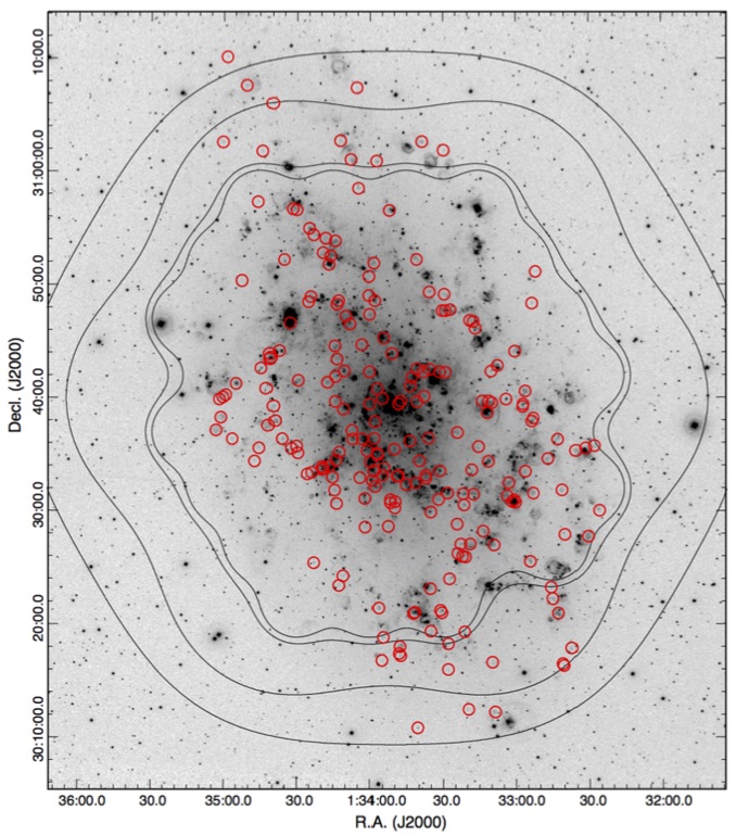
Figure 1: Image of M33 in H$\alpha$, from the 0.6m Burrell Schmidt telescope at Kitt Peak, with the locations of 217 SNRs and SNR candidates identified by Long et al. (2010) and/or Lee & Lee (2014a) indicated. See Long et al. (2018) for an optical spectroscopic assessment of many of these candidates. The contours show, from the inside to the outside, the sky regions covered by the high- and low-frequency 5 GHz bands and by the high- and low-frequency 1.4 GHz bands. Most of the SNRs are covered by both frequencies, while only a single SNR falls completely outside our radio coverage.

It has been twenty years since the G99 radio survey of M33 was published. In this paper, we describe the results of a new, deep, multifrequency radio survey of M33 carried out with the Jansky Very Large Array (JVLA). Our primary purpose is to identify radio SNRs in M33 in order to better understand the radio properties of SNRs as a class, but of course many other sources have also been detected, including thermal H II regions, X-ray binaries, background sources, and even diffuse thermal emission from the ISM of M33.

We provide an overview of the radio observations and data processing in the next section (deferring the full details of the new algorithms used for source detection and flux density measurements until Appendix A). This is followed in section 3 by an analysis of the detected radio source populations relative to optical and X-ray source catalogs and the SNR catalogs in particular. Section 4 explores how the class properties of this unique SNR sample comports with current models for remnant radio emission, while Section 5 summarizes our conclusions.

Table 1: Grid of M33 JVLA Pointing Centers

Decl. (J2000)	R.A. (J2000)
1.4 GHz
$+$30:24:24	$\cdots$	01:34:34	$\cdots$	01:33:11	$\cdots$	$\cdots$
$+$30:40:00	01:35:16	$\cdots$	01:33:53	$\cdots$	01:32:30	$\cdots$
$+$30:55:36	$\cdots$	01:34:34	$\cdots$	01:33:11	$\cdots$	$\cdots$
5 GHz
$+$30:22:00	$\cdots$	01:34:30	01:34:00	01:33:30	$\cdots$	$\cdots$
$+$30:27:00	$\cdots$	01:34:45	01:34:15	01:33:45	01:33:15	01:32:45
$+$30:32:00	01:35:00	01:34:30	01:34:00	01:33:30	01:33:00	01:32:30
$+$30:37:00	01:35:15	01:34:45	01:34:15	01:33:45	01:33:15	01:32:45
$+$30:42:00	01:35:00	01:34:30	01:34:00	01:33:30	01:33:00	01:32:30
$+$30:47:00	01:35:15	01:34:45	01:34:15	01:33:45	01:33:15	01:32:45
$+$30:52:00	01:35:00	01:34:30	01:34:00	01:33:30	01:33:00	$\cdots$
$+$30:57:00	$\cdots$	01:34:45	01:34:15	01:33:45	01:33:15	$\cdots$

2 Observations and Data Processing

Observations of M33 with the JVLA were obtained at both 1.4 GHz and 5 GHz. The 1.4 GHz observations were taken under proposal 12A-403 in A-configuration (October 2012), B-configuration (July–August 2012), and C-configuration (January–April 2012). A total of 16 hrs, 32 hrs and 16 hrs of integration time (14.0, 28.2, 12.1 hrs on source) were taken in the A, B and C configurations, respectively. Seven fields of view were required to cover the central area of M33 at 1.4 GHz. The field centers of the seven 1.4 GHz pointings are listed in the top portion of Table 1. The field centers are staggered in a hexagonal pattern (as indicated by the table layout) to produce roughly uniform sensitivity across the galaxy.

The 5 GHz observations were obtained as part of proposal 13A-291 in C-configuration in June and July of 2013 for a total of 48 hrs integration time (43.2 hrs on target). The C-configuration was chosen to give a 5 GHz spatial resolution similar to that of the 1.4 GHz B-configuration, which was utilized for the bulk of the low frequency observations. Forty-one pointings were required at the higher frequency to cover the main body of M33 due to the smaller field of view at 5 GHz. The 5 GHz field centers are also listed in Table 1 (bottom).

The coverage is indicated on an optical image of the galaxy in Figure 1. The areal coverage for the 1.4 GHz observations is significantly larger than for the 5 GHz observations. The 5 GHz sky area was limited by the allocated observing time, with the observations optimized to cover the footprint of the Chandra  M33 survey. The quality of spectral indices is much better where 5 GHz data are available, but the entire region (including areas with only low-frequency 1.4 GHz data which thus lack any spectral index information) has been analyzed for this paper. The areal coverage is 0.85, 0.64, 0.40, and 0.37 square degrees in the four frequency bands centered at 1.3775, 1.8135, 4.679, and 5.575 GHz.

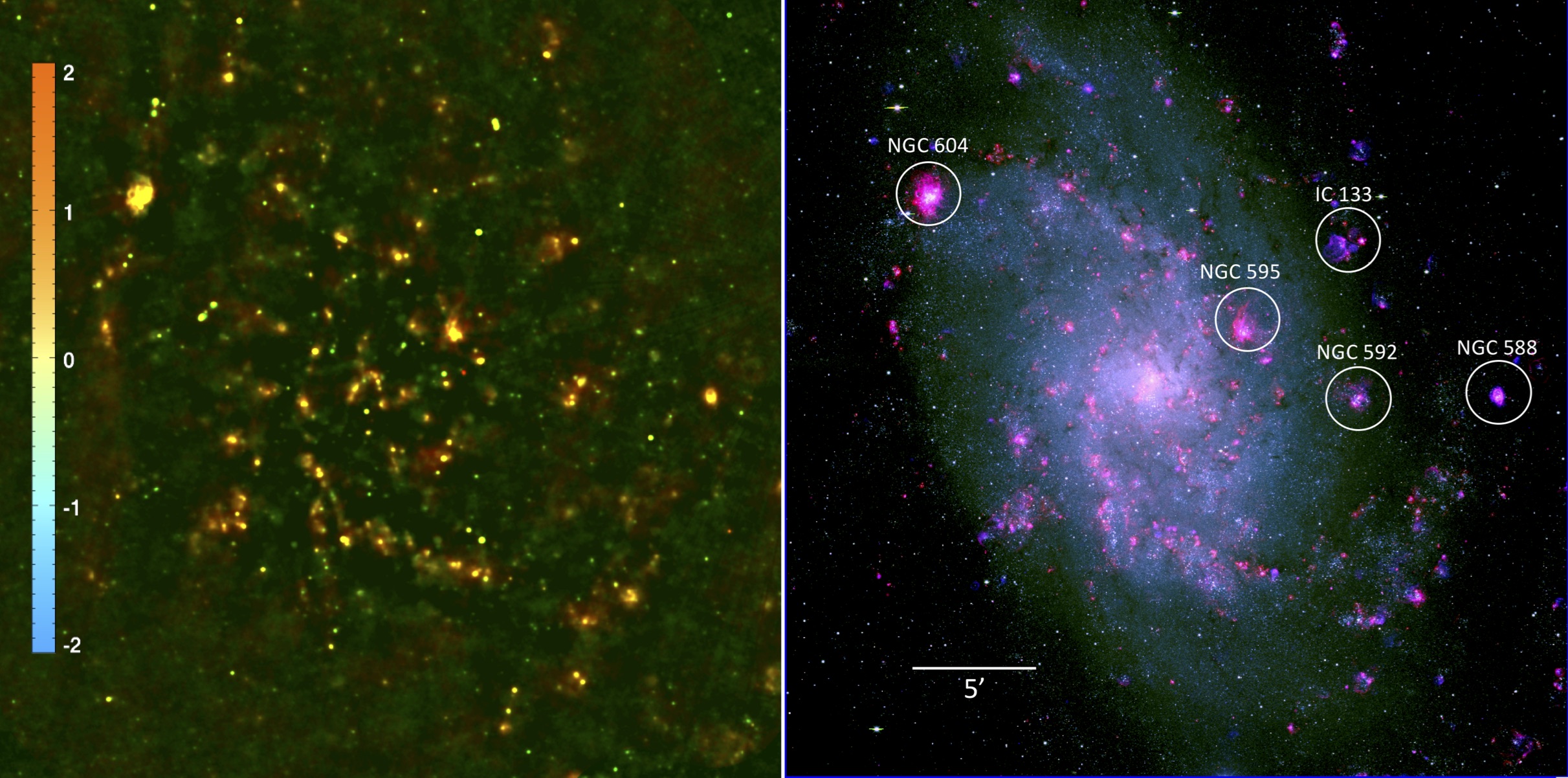
Figure 2: A radio–optical overview of M33. The left panel shows our radio data over the inner galaxy, where the gradations in color indicate changing spectral indices for the radio emission as indicated by the color bar at left. Most H II regions appear yellow, indicating a flat spectral index, while many faint green and blue (steep spectrum) sources are either background objects or SNRs. The right panel, shown to the same scale, is LGGS optical data for M33, including H$\alpha$ in red and V and B continuum images in green and blue to show the galaxy. Some of the large, named giant H II regions are labeled for reference.

The JVLA 1.4 GHz band spans 1 to 2 GHz while the 5 GHz band spans 4 to 6 GHz. These wide bandpasses present some challenges for imaging, including significant radio-frequency interference (RFI) as well as large changes to the effective field of view and resolution over the bandpass. The RFI was dealt with by severely clipping the affected portions of the uv-data using the AIPS task ‘CLIP’. The frequency-dependent primary beam required imaging and self-calibrating at each of 16 intermediate frequencies (IFs) separately. Each IF covered a frequency range of 64 MHz and 128 MHz at 1.4 GHz and 5 GHz, respectively. Images were cleaned using the AIPS task ’IMAGR’. At 1.4 GHz, multiple overlapping fields were simultaneously cleaned to remove distortions created by the spherical sky, with typically 126 fields used to cover the primary beam area. At 5 GHz a single field was sufficient for the cleaning. The images at different pointings from each IF were coadded after cleaning using optimal weighting determined by the primary beam to form a single flat image (Becker et al., 1995). The images from the individual IFs were then summed in various combinations to form images with longer integration times.

After processing in AIPS, the images at each frequency were convolved to a fixed round beam with FWHM 5.9″. This reduced the resolution of the final images, but using a fixed resolution resulted in a significantly better catalog than retaining the variable PSF sizes and shapes as a function of frequency. The fixed resolution improved both the consistency of the multi-resolution sky subtraction and filtering step (described below) as well as the accuracy of the flux densities and spectral indices.

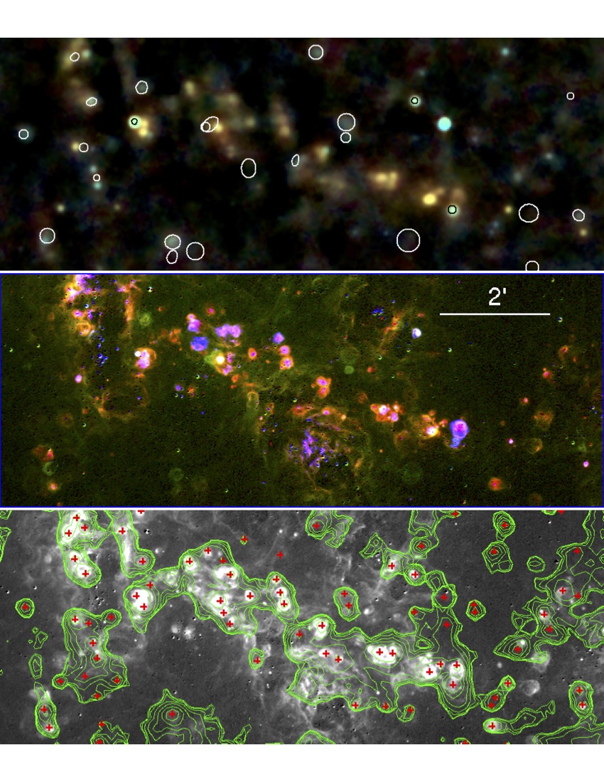
Figure 3: This figure shows a 4.4′ by 10.7′ region of the southern spiral arm in M33. The top panel is the color radio spectral index map from Fig. 2. Locations for optically-detected SNRs are shown as white ellipses (although the three objects projected against bright radio emission are shown as black); many can be identified by cross-referencing to the middle panel that shows a three-color image of LGGS continuum-subtracted emission line data, with H$\alpha$ in red, [S II] in green, and [O III] in blue. SNRs show as greenish areas (strong in [S II]). (SNRs that are bright in all three optical bands will, of course, show as white in the middle panel.) No regions are overlaid on this panel so the optical structures can be seen without interference. The bottom panel is a continuum-subtracted H$\alpha$ image from LGGS, shown with log scaling to increase the dynamic range. The green overlay shows radio contours from the 1.4 GHz data, with the following levels: 1.6, 3.2, 6.4, 12.8, 25.6, 51.2, and 102.8 $\mu$Jy. Red crosses mark the positions of radio sources from our catalog in this region. Some of the complexity of making associations between radio sources and either H II regions or SNRs can be seen here.

In Figure 2 (left), we show an overview of the radio data, where the color in the map represents the spectral index of each source, as shown by the scale bar. In Figure 2 (right), we show an optical image of the galaxy at the same spatial scale for comparison. One can see that many of the brightest radio sources correspond to H II regions in M33, and most of these have a yellow color in the left panel, indicating fairly flat (thermal) radio spectra. However, close inspection shows H$\alpha$ nebulae that align with green radio sources in the left panel, indicative of steeper non-thermal spectra. Many of these are optical SNRs and will be discussed below. Many faint green-to-turquoise (steep) sources do not have obvious optical counterparts and likely represent background sources. In some of the larger complexes of H$\alpha$ emission, a more diffuse component of radio emission is also visible.

These new radio images are deep enough that they are complex and crowded, particularly in the central regions and southern spiral arm of the galaxy. To provide more context to this comparison between the radio maps and the optical data, we show an enlarged section of the complex southern spiral arm region in Figure 3. The top panel of this figure shows the two-color radio map of the region as shown in Figure 2 (left), with white ellipses at the positions of optical SNRs from L18 for reference. These regions can be referenced to the middle panel of the figure, where we show a three-color version of the LGGS optical continuum-subtracted emission line data for the region, with H$\alpha$ shown in red, [S II] in green, and [O III] in blue. The graytone background in the bottom panel is a version of the LGGS H$\alpha$ data where we have scaled and subtracted the continuum and displayed it on a log scale to enhance the dynamic range. Overlaid on this panel in green are contours from the 1.4 GHz radio map as indicated in the figure caption. The red crosses indicate positions of radio peaks in the catalog, as described in the next section. Correspondences with both SNRs and H II regions are clearly seen, but the difficulty of making unique associations in some cases is evident. Often the SNRs appear in regions of extended or adjacent H II emission.

2.1 Construction of the Radio Source Catalog

The majority of the emission in our radio maps is in the form of point or discrete sources. Hence, we have constructed a catalog of these sources to permit comparisons between these new radio data and catalogs at other wavelengths.

The radio source catalog was created by averaging the data in the 1.4 GHz and 5 GHz bandpasses to produce a single detection image. For the 1.4 GHz data, the entire bandpass was used, and 14 of the 16 125-MHz channels from the 5 GHz observations were used. (Channels 1 and 2 of the 5 GHz data were contaminated by RFI.) The 5 GHz and 1.4 GHz bands are equally weighted in the combined image, resulting in source lists that are not a strong function of the source spectral index. This equal weighting is not optimal for a typical extragalactic source (which has a power law spectrum $\nu^{\alpha}$ with $\alpha\approx-0.7$) but is a reasonably “spectrum-neutral” strategy for the source detection, which is more appropriate for our study.

The complexity of the radio emission causes a significant spatial variation in the background level with position. We developed a multi-resolution (median pyramid) image processing algorithm, both for use in source detection and to subtract the background from the images to make the source detection threshold more uniform. The multi-resolution median pyramid images were also used for both source detection and flux density measurements for the sources. We describe this new and somewhat complex algorithm in detail in Appendix A.

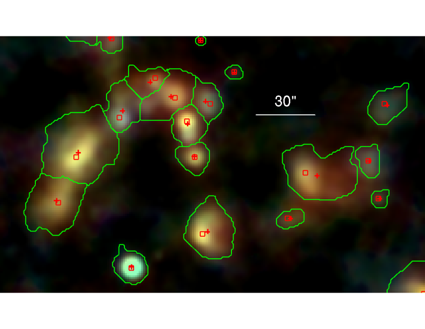
Figure 4: This figure shows a region near the M33 nuclear region (upper left) and just to the west, demonstrating the different elements of the radio catalogs. The green outlines indicate the radio emission islands described in the text. The red crosses indicate the positions determined for the mean of each island, while the red squares indicate the cataloged “peaks” determined by the algorithm. These can be slightly offset from each other, depending on the complexity of the enclosed emission, although for most isolated islands they are nearly identical.

An island map (segmentation map) technique is used to indicate image regions where sources were detected. Figure 4 shows an enlargement near the complex nuclear region as an example of the results of this process. Here we provide a brief summary of the algorithm used to compute the islands and the positions listed in our catalog:

• The detection image is separated into a stack of images of equal size that have structures on scales ranging from compact to very extended. The sum of this stack is equal to the original image.

• At each stack level, the local rms noise is estimated, and pixels that exceed that noise by a factor of two are included in a segmentation map indicating potential source positions. Contiguous pixels are grouped into “islands” for different sources.

• The lowest resolution image from the stack is treated as a variable sky level and is not used for source detection or in flux calculations.

• Overlapping islands at different levels are merged and/or split as necessary to group them with islands at other levels. When this is complete, each pixel of the image is assigned to a single island in one or more levels of the stack or is not assigned to any source.

As seen in Fig. 4, the resulting islands can be irregular in shape and sometimes include what to one’s eye might appear as two or more sources (or a point source with adjacent more diffuse emission). However, in complex regions the islands usually fit together snugly and thus capture all of the radio flux from the region.

Each island corresponds to a single source in the catalog. The fluxes for sources are calculated by computing similar multi-resolution image stacks for each frequency band image. Pixels that are assigned to an island at a given resolution level are included in the summed flux for the source. Note that the island size may change at each resolution level, which effectively leads to an adaptive weighting of the image pixels that depends on the source profile. There is a PSF-dependent correction factor (close to unity) for flux that spills outside the island. The island shapes are identical for all the different frequency bands (as are the PSFs after the beam sizes have been matched), which leads to accurate and reliable spectral indices. See Appendix A for further details.

The moments of the mean detection-image flux densities in each island are used to determine the centroid position and a representative elliptical morphology (FWHM major and minor axis and position angle) for each source, as listed in the catalog. The size quoted in the catalog has not been corrected for the round 5.9″ FWHM beam size. For an unresolved source the major and minor axes will be approximately equal to 5.9″. Note that the size is not constrained to be larger than this value; sources with sizes smaller than the beam width (due to noise fluctuations) can have integrated flux densities smaller than their peak flux densities. In such cases the peak flux density may be a more reliable estimate of the source brightness.

The integrated flux densities for each of four bands (two from 1–2 GHz and two from 4–6 GHz) are fitted with a power law to determine the spectral index $\alpha$ for each source, $F_{\nu}=F_{\mathrm{int}}(\nu/\nu_{p})^{\alpha}$. The noise in the band fluxes is used to determine the errors in $F_{\mathrm{int}}$ and $\alpha$. The pivot frequency $\nu_{p}$ is chosen as the frequency where the covariance between $F_{\mathrm{int}}$ and $\alpha$ is zero, which also is the frequency of the optimal signal-to-noise $F_{\nu}/\sigma(F_{\nu})$. The spectral index fit is constrained to $-3\leq\alpha\leq 3$; sources with spectral indices at these limits have $\sigma(\alpha)=0$.

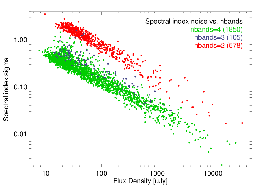
Figure 5: A comparison of the noise in the computed spectral index as a function of the source brightness and the number of frequency bands with data for a given source. In the outer parts of the galaxy, where only two frequency bands are available, the spectral index uncertainties are six times larger than in the central regions, where four frequency bands are measured. Only the brightest sources with two-band detections have accurately measured spectral indices.

The accuracy of the spectral indices degrades in the outer region where fewer frequency bands are available (Fig. 5). In the center of the galaxy, sources are measured across the full 1–6 GHz bandpass. The frequency-dependent field of view reduces the sky area covered at higher frequencies, so outer regions of the galaxy are covered by fewer frequency bands (Fig. 1). The uncertainty in the spectral index is determined by both the signal-to-noise of the flux density measurements and by the frequency lever-arm of the data. The small region with three bands has only slightly worse noise than the four-band data, but the two-band data (with measurements only in the 1–2 GHz bandpass) has spectral index errors that are six times larger. As a result, only the brightest sources with two-band detections have accurately measured spectral indices. (Obviously the outermost region with only a single band detected has no spectral index information at all.) Fortunately, the majority of the sources are found in the inner region of the galaxy where there is full frequency coverage.

In addition to the island centroids, the catalog also includes the peak flux density and the position of the peak for each island. These values are computed from the detection image, just as for the flux-weighted positions. The peak is simply the brightest pixel in the island after background subtraction. The position of the peak (which may differ from the flux-weighted mean in asymmetrical sources) is determined in the sharpest channel of the multi-resolution image stack where the source is detected. This means it represents the position of the peak for the most compact source component. We found that this choice gives more accurate peak positions in crowded regions.

The results are summarized in Table 3, which includes all sources detected at a signal-to-noise $F_{\mathrm{int}}/\sigma(F_{\mathrm{int}})\geq 4$. It also includes seven sources that fall below that detection threshold but that have associations in external X-ray or H II region catalogs; those sources are flagged as sub-threshold objects. A full description of the columns in the table is found in Table 6.

Our final catalog contains 2875 sources with 1.4 GHz flux densities ranging from about 2.2 $\mu$Jy to 0.17 Jy. (The faintest 1.4 GHz fluxes are for objects with inverted spectra that are brighter at 5 GHz.) Of these, 670 have spectral indices determined with an accuracy $\sigma(\alpha)\leq$ 0.15. Essentially all sources with 5 GHz data (2/3 of the catalog) and fluxes in excess of 150 $\mu$Jy have well-measured spectral indices. The typical noise in the integrated flux density is $<5$ $\mu$Jy, although there are a few crowded regions where the noise is significantly higher (Fig. 6).

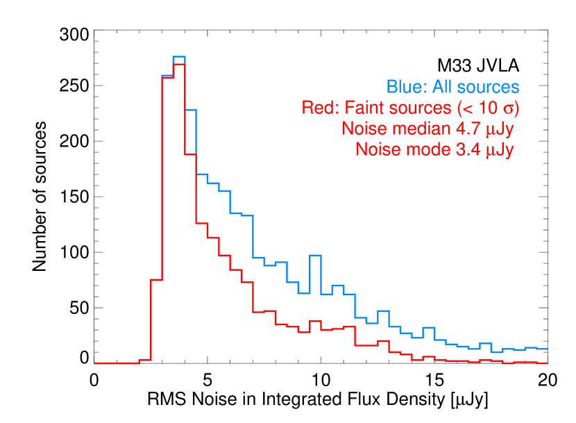
Figure 6: The distribution of noise values in the integrated flux density in the JVLA M33 catalog. The distribution has a peak near 3–4 $\mu$Jy with an extended tail of higher noise values. However, the tail is contributed mainly by bright sources (that are well above the detection threshold). For sources detected at $<10\sigma$, the noise mode is 3.4 $\mu$Jy and the median is 4.7 $\mu$Jy. Over most of the survey area our catalog is complete to $\sim 20$ $\mu$Jy($4\sigma$).

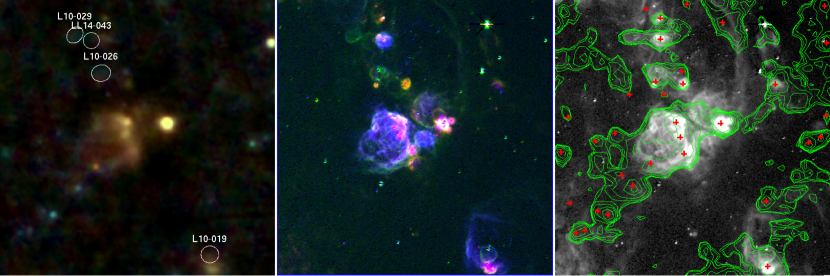
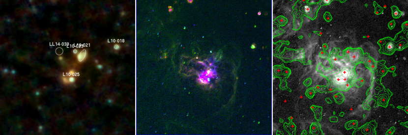
Figure 7: Two 5′ regions centered on giant H II regions in M33. (top) IC 133, and (bottom) NGC 592. The panels and labeling are similar to Fig. 3. Note that both regions include multiple radio peaks (red +’s in the right panel), and the radio contours show connections from the main optical H II region to more extended structure with additional radio peaks.

With the sensitivity and resolution of these new data, some of the larger optical emission structures like giant H II regions or H II emission complexes incorporate numerous individual radio emission peaks. Figure 7 shows two examples, IC 133 and NGC 592, where the color coding and labeling are similar to those in Figure 3. IC 133 shows a bright, relatively high-excitation (strong [O III]-emitting) bi-lobed structure in the optical with five radio peaks on portions of the main nebula. The radio contours extend to the lower left, incorporating another eight radio peaks that are listed in the catalog. Several optical SNRs are indicated nearby but are not directly related to IC 133. In contrast, NGC 592 has a very bright core of optical emission with a number of fainter loops of surrounding emission that are mapped reasonably well by the radio contours, including a faint arm of emission to the west. Several SNRs are associated with this region as well. Several radio peaks correspond with the bright core region, while the extended radio contours incorporate a dozen or more additional radio peaks.

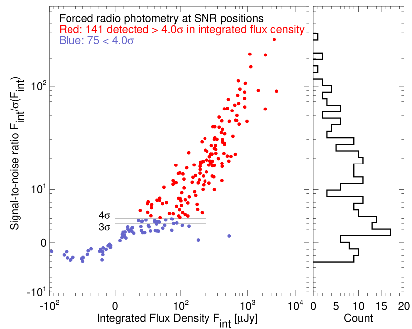
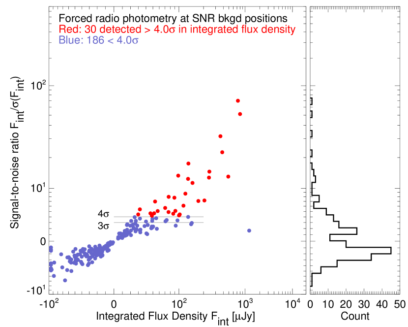
Figure 8: The signal-to-noise as a function of the integrated flux density $F_{\mathrm{int}}$ for the SNR forced photometry (top) and background photometry using SNR regions shifted by 1 arcmin (bottom). Note that the measured flux densities can be negative for non-detections. The histogram on the right shows the distribution of signal-to-noise values. The false positions are obviously much fainter, but sometimes sources are “detected” due to random coincidences with radio sources in the crowded field. Eight simulations like the one at the bottom were performed to determine the signal-to-noise distribution of chance matches.

2.2 Forced Photometry Catalog at Optical SNR Positions

The radio catalog described above was constructed without any reference to the positions of known optical SNRs in M33 (although many of the remnants were detected). However, we have also constructed a separate catalog of radio properties at the positions of known optical SNRs by integrating the radio images over the elliptical region determined for each optical SNR, as measured previously by either L10 or LL14. (When a SNR appeared in both lists, we somewhat parochially adopted the regions of L10.) This method allows us to establish either measured flux densities or appropriate upper limits for the radio emission from all SNR candidates, whether or not a radio source was independently detected at the SNR position. We will refer to this version of the SNR radio data as the “forced photometry” SNR extraction catalog.

The calculations of flux densities, spectral indices, and flux-weighted positions proceeds much as described above for the radio catalog. The island map for the forced photometry catalog is determined from the elliptical regions in the optical SNR catalog rather than from the radio map itself. Since the island map makes no reference to the radio morphology, we do not have multi-resolution islands but instead sum the radio flux density over the entire region using the single background-subtracted image in each radio band. The catalog does not include the radio peak information (which was not found to be useful) but does include the input positions for the regions along with the radio-flux-weighted centroid positions.

Associations between SNRs and objects in our master radio catalog are determined by the overlap between the radio island map and the SNR island map. Many SNRs have unambiguous matches with cataloged radio sources, but there are also ambiguous cases where a single SNR island overlaps several radio islands and vice versa. The information on the overlapping sources and a flag that captures information on the ambiguity of the association are also included in the table.

Of the 217 SNRs and SNR candidates in the merged list of L18, 216 are in the region covered by our radio images (see Fig. 1). The only object falling completely outside the radio region is LL14-195. There are 188 SNRs in the central region covered by both the 1.4 GHz and 5 GHz frequency bands plus two more that have data from 1.4 GHz and the low-frequency 5 GHz bandpass only. Of the 26 sources that have only 1.4 GHz data, only one (L10-003) has a reasonably accurate spectral index; we have little spectral index information in the outer region of the galaxy.

We find that 155 of the 216 SNRs and candidates are detected above 3$\sigma$ at radio wavelengths, a detection rate of 72%. That detection rate rises to 76% (145 of 190) in the central region where we have full frequency coverage. The remainder have radio upper limits from the forced photometry exercise. (Some of the sources below the $3\sigma$ threshold are also likely to be detected: there are, for example, 12 $2\sigma$ detections discussed further below.) Of the 155 $3\sigma$ radio-detected SNRs, 126 came from the list of 137 candidates in L10, while 29 came from the 79 SNRs that were first suggested as candidates by LL14. The fact that a much lower percentage (37% versus 92%) of the extended list of SNR candidates identified by LL14 were detected in the radio is undoubtedly related to the fact that many of the LL14 candidates are optically fainter than those in the L10 list.

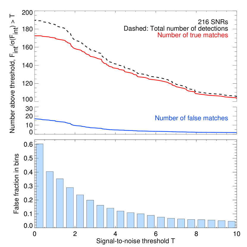
Figure 9: The number of false detections in the SNR forced-photometry table as a function of signal-to-noise. The top panel shows the cumulative number of detections (dashed line), the estimated number of false detections (blue line), and the number of remaining true matches (red line) as a function of the signal-to-noise. The bottom panel shows the fraction of false detections in signal-to-noise bins. Using a $3\sigma$ detection threshold, the contamination rate is low: fewer than 15% of the SNRs with $3\sigma<F_{\mathrm{int}}/\sigma(F_{\mathrm{int}})<3.5\sigma$ are expected to be the result of chance.

An important consideration in setting the detection threshold at $3\sigma$ is the expected rate of chance coincidences between the SNR islands and the radio map. The radio images are sufficiently crowded that randomly placed ellipses will sometimes fall on radio sources. This is particularly true in the center of the galaxy and in the spiral arms. We estimated the rate of chance radio detections by shifting the SNR islands by $\pm 1$ arcmin in RA and Declination. The size of the shift was chosen to be larger than the largest island’s major axis. The shift is large enough to move off the local object while still being small enough to be sampling the same environment (spiral arm, galaxy center) as the true SNR position. The shifted calculations also use the same distribution of region sizes as the real catalog, which has a significant influence on the background rate. Eight shifts were done, including shifts only in Declination, only in RA, and in both RA and Dec. For every shift, forced photometry was performed on all the regions using exactly the same approach as for the real positions.

A comparison between the measured flux densities for the real SNR regions and a typical example of the shifted SNR region fluxes is shown in Fig. 8. While positive detections are much rarer at the shifted positions, they are common enough that they cannot be ignored.

All eight shifted catalogs for each object class were combined to compute the distribution of the signal-to-noise, $F_{\mathrm{int}}/\sigma(F_{\mathrm{int}})$, for random positions on the sky. With eight simulations of the random detections, the simulated noise distribution is reasonably well determined. Given the cumulative distribution of the number of sources exceeding a given signal-to-noise ratio, we then compute for every source in the real catalog the probability that a random source of equal or greater flux would be detected.

Finally we compare the cumulative distribution of the actual number of sources detected as a function of the detection threshold with the cumulative distribution of the random detection probability above that threshold (Fig. 9). That gives an estimate of the number of false detections that are included as a function of the detection threshold.

We conclude that a detection threshold of $3\sigma$ leads to acceptable contamination by false detections. Of the 141 SNRs above $4\sigma$, $\sim 5$ are likely to be due to false matches. Adding the SNRs between $3\sigma$ and $4\sigma$ increases the number detected by 14 while adding only 2 additional false matches. Even detections between $2\sigma$ and $3\sigma$ are likely to be fairly reliable, with $\sim 75$% of the 12 detections in that range expected to be true detections. (These coincidence rates are lower than intuition might suggest because the high true detection rate for SNRs means that there have been relatively few “rolls of the dice” at empty sky positions.)

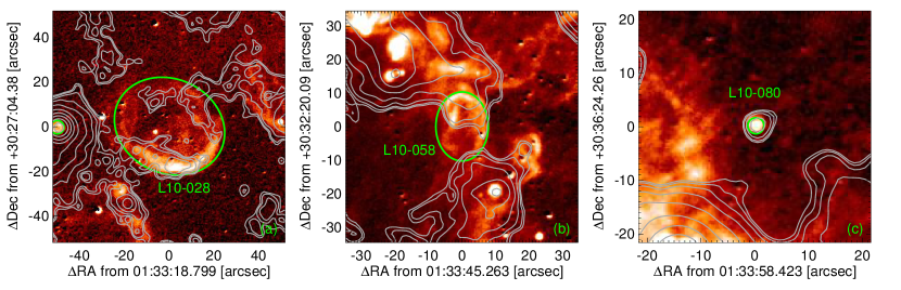
Figure 10: The H$\alpha$ and combined radio images for several SNRs for which coincident radio emission is present but fails to rise above the forced photometry detection threshold. The image is the LGGS H$\alpha$ data, the green ellipses show SNRs, and the contours are for the combined 1.4 plus 5 GHz image at levels 1.6, 3.2, 6.4, …, 819.2 $\mu$Jy. (a) In L10-028, only the brightest part of the optical shell has a radio counterpart. (b) L10-058 shows a close morphological match of the optical and radio images but the higher background induced by the nearby bright source hampers detection. (c) Source L10-080, the smallest diameter remnant in the catalog, has a clear sub-threshold counterpart that falls just below the $3\sigma$ detection threshold (at $2.7\sigma$).

The basic characteristics of the SNRs as well as results of our forced photometry extraction are presented in Table 4, where the non-radio data are from L18. The [S II]:H$\alpha$ column in this Table indicates whether optical spectra exist and whether these showed a [S II]:H$\alpha$ ratio of 0.4 or greater. The X-ray column indicates whether an object was detected at 3$\sigma$ or greater with Chandra  by L10 or with XMM-Newton by Garofali et al. (2017). A full description of the columns in the table is found in Table 7. Our forced photometry radio catalog of SNRs contains 178 SNRs that have been optically confirmed by the [S II]:H$\alpha$ criterion; there are another 27 objects that have spectra but show lower [S II]:H$\alpha$ ratios, and 12 for which there are not yet any optical spectra. A total of 112 of the objects are also detected in X-rays.

The SNR forced-photometry table also identifies radio sources from the master catalog (Table 3) that have detection islands that overlap the SNR regions. In cases where more than one radio source overlaps the SNR, all the matches are listed. Multiple matches are sorted by the number of overlapping pixels, so the radio source sharing the largest number of pixels with the SNR region is listed first. Similarly information is included in the radio catalog for cases when a radio source overlaps one or more SNRs, and the same information is available for radio matches to the forced photometry X-ray catalog (described below). The Sflag (Table 3) and Rflag (Tables 4 and 5) columns are bit flags with values that help determine whether a match is reliable. For the Sflag column, for example, the bit values $b$ indicate that

• $b=1$: the SNR has a radio match,

• $b=2$: the match is unambiguous, so only one radio source matches the SNR, and

• $b=8$: the match is mutually good, meaning that the best radio source for this SNR also has this SNR as its own best match, where “best” is determined by the number of overlapping pixels between the islands.

The most reliable matches will have flag bit 8 set. All of those will have bit 1 set as well, and most of them will also have bit 2 set. Flag values of 9 and above indicate good matches, with the best having flag values of 11. The distributions of the values of Sflag (in the radio catalog) and Rflag (in the SNR and X-ray catalogs) are shown in Table 2.

Table 2: Flag Value Counts in the Radio and SNR Catalogs

Value	6exSflag
Radio	6exRflag
SNR	7exRflag
X-ray	Meaning
0	2728	75	342	10emNo match
1	0	1	1	10emAmbiguous matches
3	18	11	20	10emSingle match but not mutually good
9	17	19	22	10emMutually good match
11	112	110	277	10emSingle, mutually good match

Of the 155 SNRs detected at 3$\sigma$ in the forced photometry catalog, 134 are associated with a source in the master radio catalog. Of these, there are 19 sources in the SNR catalog associated with two (or three) radio sources. There are 21 SNRs detected as faint sources in the forced photometry catalog that are not found in the master catalog. Since the master radio catalog has a $4\sigma$ detection limit (compared with $3\sigma$ for the forced photometry), it is not surprising that there are sources below the radio catalog limit.

In some cases where the forced photometry does not yield a $3\sigma$ detection, radio emission is still apparent at the optical remnant location. These cases arise from the incommensurability of the flux density distribution in the optical and radio bands, the presence of a nearby bright radio source, or radio emission just below the detection threshold. Examples of these cases are shown in Figure 10. In some cases (L10-028, L10-030, LL14-038, and L10-131), only the brightest part of the optical shell has coincident radio emission, and the overall source falls below threshold (Fig. 10a). In other cases (L10-058, LL14-096, L10-132, LL14-142) a bright, nearby (and apparently unrelated) source raises the local background sufficiently that the radio counterpart falls below threshold (Fig. 10b). In yet other cases (LL14-125, LL14-128, L10-048, L10-080, L10-092, LL14-058), a clear radio counterpart is apparent but falls just below the threshold (Fig. 10c); note that the division between the latter two categories is somewhat arbitrary. In summary, over one-quarter of the remnants not listed here as having radio emission do have modest levels of radio flux associated with them that a deeper and/or higher resolution survey would definitely have detected.

2.3 Forced Photometry Catalog at Chandra X-ray Positions

The list of X-ray source positions from the ChASeM33 catalog of Tüllmann et al. (2011) was also used to construct a forced-photometry catalog with radio flux densities. The procedure followed was very similar to the SNR forced-photometry catalog described above. The resulting table (shown as a sample in Table 5) has a $3\sigma$ threshold for radio detections (but includes the radio measurement regardless of the signal-to-noise). It includes information from the X-ray catalog including the diameter and count rates in various energy bands. The Rflag column is defined exactly as for the SNR forced photometry table, with values of 8 or greater indicating confident (or at least unconfused) associations. The format is similar to Table 4; a full description of the columns is found in Table 7.

Of the 662 X-ray sources, 319 are detected in our radio survey. All of these X-ray sources fall in the region that has both 1.4 GHz and 5 GHz radio data, and 102 of the detections have radio spectral indices determined to an accuracy $\sigma(\alpha)<0.15$.

2.4 Identification of H II regions

Many of the radio sources in the catalog are associated with star-forming H II regions, with optically thin thermal bremsstrahlung radiation having a spectral index $\alpha\sim 0$. In order to determine which sources in our radio catalog are associated with H II regions, we have computed the H$\alpha$ surface brightness over the radio island regions for each source in the catalog using the H$\alpha$ image obtained by one of us (PFW) using the Burrell Schmidt camera at Kitt Peak in Arizona (cf. L10). The tables for both the radio catalog and the forced photometry catalogs include the total H$\alpha$ flux, $F(\mathrm{H}\alpha)$, and the average flux surface brightness (per square arcsec), $\Sigma(\mathrm{H}\alpha)$.

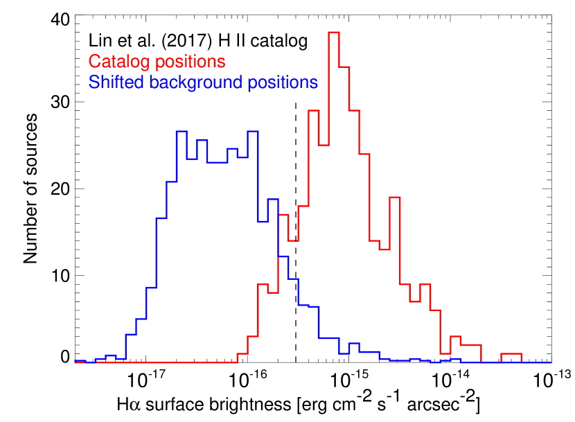
Figure 11: A comparison of the H$\alpha$ surface brightnesses for the Lin et al. (2017) H II region sample (red) with the background H$\alpha$ surface brightness distribution (blue). The surface brightnesses are averaged from our H$\alpha$ image over the region in the catalog. The background distribution was determined by shifting the true catalog positions by 1 arcmin to five different nearby positions. We conclude that a surface brightness threshold $\Sigma(\mathrm{H}\alpha)>3\times 10^{-16}\,\mathrm{erg\,cm^{-2}s^{-1}arcsec^{-2}}$ (dashed line) separates H II regions from background sources with a contamination rate of 10% by background sources.

To determine an appropriate $\Sigma(\mathrm{H}\alpha)$ threshold to identify H II regions, we have used the Lin et al. (2017) catalog with spectroscopic observations of 413 star-forming regions in M33. This catalog is not a complete compilation of H II regions in M33 because its sample was shaped by the constraints of the fiber-fed spectrograph used for these observations. Despite that limitation, it represents a good subset of M33 ionized regions for our analysis.

Figure 11 compares the H$\alpha$ surface brightnesses for the Lin et al. (2017) fiber positions with the background distribution computed from a set of shifted regions. Five different shifts of 1 arcmin were used to determine the background distribution. We conclude that a surface brightness threshold $\Sigma(\mathrm{H}\alpha)>3\times 10^{-16}\,\mathrm{erg\,cm^{-2}s^{-1}arcsec^{-2}}$ separates H II regions from background sources, generating a reasonably reliable and complete sample. The background rate is not negligible (about 10% of the background positions exceed this threshold), but some contamination is unavoidable in a galaxy this crowded with star formation.

3 Analysis

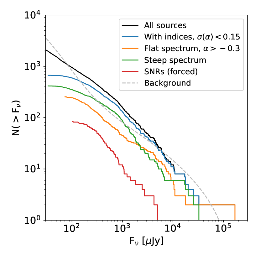
Figure 12: The number of sources with flux densities greater than F_ν for the entire catalog (in black) and various subsamples in other colors. Here flat-spectrum sources are defined as sources with spectral index $\alpha>-0.3$ and steep-spectrum as $\alpha\leq-0.3$. Only sources with accurately measured spectral indices, $\sigma(\alpha)<0.15$, are included in the flat/steep samples. The flux distribution for the SNR forced photometry is also shown. The dashed gray line shows the expected background counts (Smolčić et al., 2017).

In Figure 12, we show cumulative luminosity functions for the catalog and for various sub-sets thereof. The higher luminosity portions of each curve can be fitted with a straight line, but all curves show apparent “breaks” indicating limits to the completeness of the sample being plotted. It is difficult to set a single limiting flux for the survey because the background levels change with position and with the complexity of emission surrounding individual sources.

In this and other plots of the paper, we select samples of sources with accurately determined spectral indices using $\sigma(\alpha)<0.15$. One third of the radio sources fall in the outer parts of the survey where only 1.4 GHz data is available (Fig. 1). Excluding those sources, which do not have accurate indices, 90% of objects with $\mathrm{F(1.4\,GHz)}>100$ $\mu$Jy have accurate spectral indices (see Fig. 5 for details).

Background radio galaxies and AGN contribute significantly to the source counts. Figure 12 also shows the background counts expected based on Smolčić et al. (2017). Many of the brightest sources ($>10\,$mJy) are likely to be background objects, but the bulk of fainter objects belong to M33.

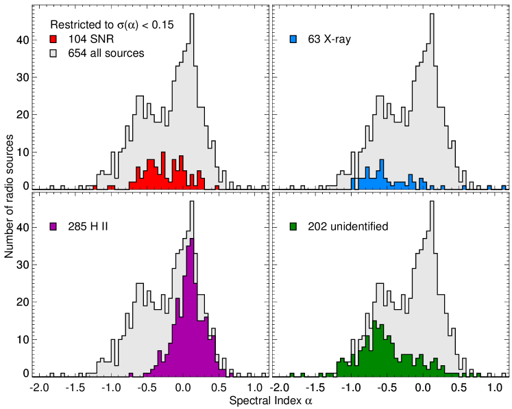
Figure 13: The distribution of spectral indices for sources whose spectral index was measured to an accuracy of 0.15 or better. The gray shaded histogram shows the entire source distribution and is the same in each panel. The four panels highlight sources associated with SNRs, H II regions, X-ray sources (excluding SNRs and H II regions), and unidentified sources not associated with known objects. Potentially confused objects with flags less than 9 (Table 2) are excluded. More than 40% of radio sources with $-0.5<\alpha<-0.2$ are associated with SNRs.

The distribution of measured spectral indices for the sources in the catalog is shown in Figure 13. It is double peaked, with one peak near spectral index 0 and one near $-$0.6, as one would expect if there were two populations of sources, one dominated by H II regions and one dominated by extragalactic sources and SNRs. The four panels of the plot show the overall distribution in gray (identical in each panel) along with the distributions for objects identified as SNRs, H II regions, X-ray sources (not including SNRs or H II  regions), and unidentified sources. There are clear differences among the different populations. Essentially all of these sources associated with H II regions have spectral indices $\alpha\sim 0$ that one would associate with optically thin, thermal free-free emission. By contrast, the sources associated with SNRs and with X-ray sources have spectral indices which are mostly negative and therefore associated with non-thermal emission. Most objects that are not SNRs or H II regions are background radio galaxies and AGN, although there are also a few radio sources associated with X-ray binaries in M33.

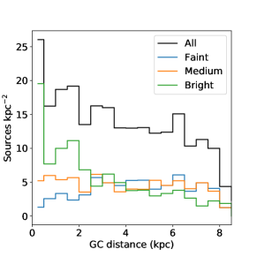
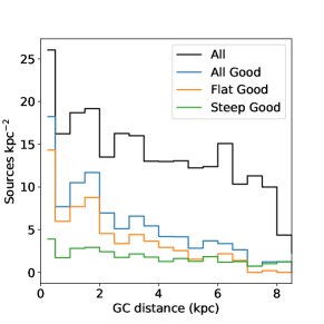
Figure 14: The surface density of sources as a function of deprojected galactocentric distance (GCD). Only sources with 5 GHz data are included. Beyond about 5 kpc the densities have been corrected for the limited portions of M33 that were observed. Both panels show the source densities for all of the sources in the catalog in black. The left panel shows the distribution of the brightest third of the sources (in green), the middle third (in orange) and the faintest third (in blue). Bright sources tend to appear closer to the center, as expected. The right panel shows the surface density for all sources with well measured spectral indices (in blue), flat-spectral indices (in orange) and steep indices (in green). The steep-spectrum source distribution is nearly flat, consistent with the majority of these sources being background AGN.

The distribution of sources as a function of deprojected galactocentric distance (GCD) is shown in Figure 14. GCDs were calculated assuming standard M33 values for the major axis position angle (23^∘) and inclination (56^∘) (see Zaritsky et al., 1989). Beyond about 5 kpc, our radio map is not complete, so all of the distributions were corrected for the fraction of the galaxy observed at each GCD. As shown in the figure, the bright sources are more concentrated (at least in terms of density) at smaller GCDs than the faint sources. This is what one would expect if a larger fraction of the faint sources were extragalactic. Indeed, there appears to be a deficit of faint sources near the center, most likely due to source crowding there. When the sources are split according to spectral index (-0.3), those with flat spectra are more concentrated toward the center, consistent with the hypothesis that most of the flat spectrum sources are due to H II emission in M33. By contrast the non-thermal sources have a flat distribution, indicating that the majority of these are background sources.

3.1 Supernova Remnants Detected in Our Radio Survey

Of the list of 217 SNRs and SNR candidates compiled by L18, 216 are in the region covered by our radio survey and 155 are detected above 3$\sigma$ via forced photometry, including 84 that have radio spectral indices with an uncertainty of less than 0.15. There are 122 of the detected objects where spectroscopy has confirmed [S II]:H$\alpha$ flux ratios exceeding 0.4, the usual optical criterion that an emission nebula is a SNR, and of these 92 have X-ray detections.

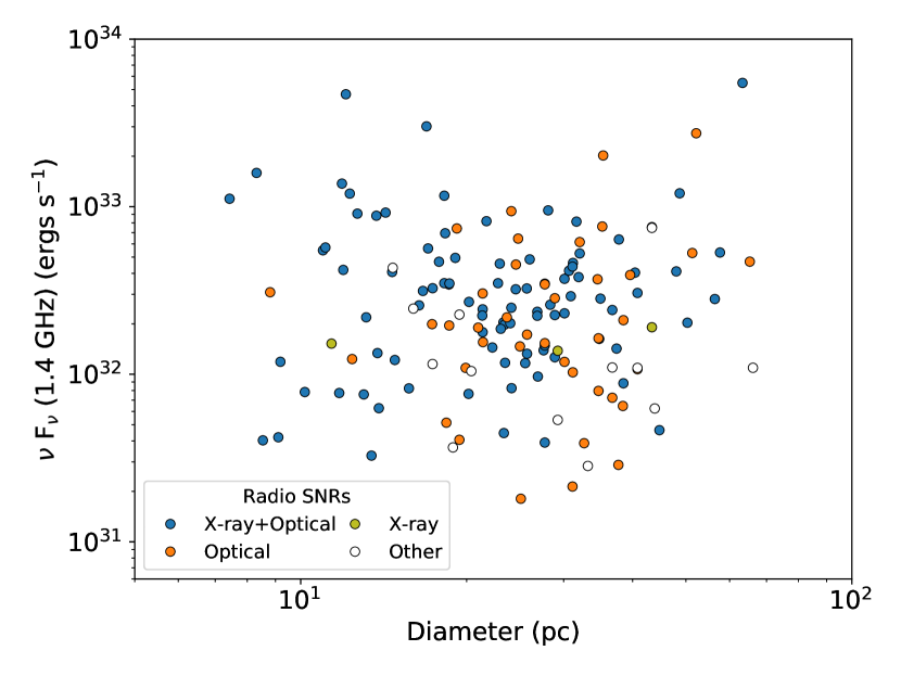
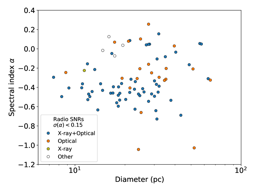
Figure 15: Left: The 1.4 GHz radio luminosity of SNRs detected through forced photometry as a function of SNR diameter. Right: Accurately determined radio spectral indices for the SNRs. The sample has been divided into objects with an X-ray detection plus optical confirmation of high [S II]:H$\alpha$ ratio (blue), objects with only optical spectroscopic confirmation (orange), objects with only an X-ray detection (green), and objects identified as possible SNRs through optical imaging, but without confirmation through spectroscopy or X-ray emission (open circles).

The derived radio luminosities at 1.4 GHz and spectral indices of these objects are shown as a function of SNR diameter in Figure 15. Neither the luminosity nor the spectral indices show a significant correlation with diameter. Radio luminosities for the entire sample and the various subsamples show very large dispersions at all diameters. Smaller diameter SNRs are not significantly brighter or fainter than those at large diameter. Similarly, radio spectral index does not appear to evolve with diameter. In contrast, a correlation between spectral index and diameter has been reported for the LMC (Bozzetto et al., 2017); we discuss this difference further in section 4.3.

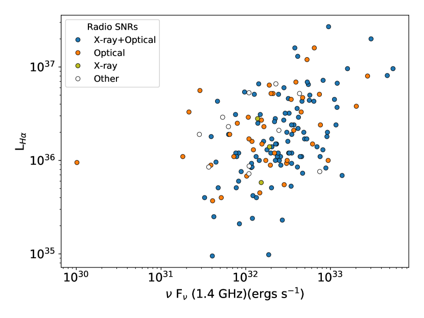
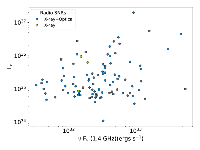
Figure 16: Left: H$\alpha$ luminosity as a function of 1.4 GHz luminosity for SNRs detected through forced photometry. Right: X-ray luminosity as a function of the 1.4 GHz luminosity. The points are color coded as in Fig. 15.

Comparisons between the 1.4 GHz luminosity and the H$\alpha$ and X-ray luminosities are shown in Figure 16. Although there is considerable scatter, there appears to be a trend between H$\alpha$ and radio luminosity. More luminous SNRs in H$\alpha$ appear to be more luminous at radio wavelengths. Whether this trend is physical is hard to determine because the scatter is large. The SNRs in M33, like those in essentially all other galaxies, were initially identified through optical interference filter imaging, and are thus surface brightness limited. Larger SNRs tend to have higher H$\alpha$ luminosities as a result. By contrast, the X-ray sample is luminosity limited. This accounts for the fact that there are almost no SNRs with L_x less than $4\times 10^{35}\rm\>\>{\rm ergs\>s^{-1}}$, the approximate limit of the Chandra survey. That said, it is interesting that the objects with highest X-ray luminosities also tend to have the highest radio luminosities.

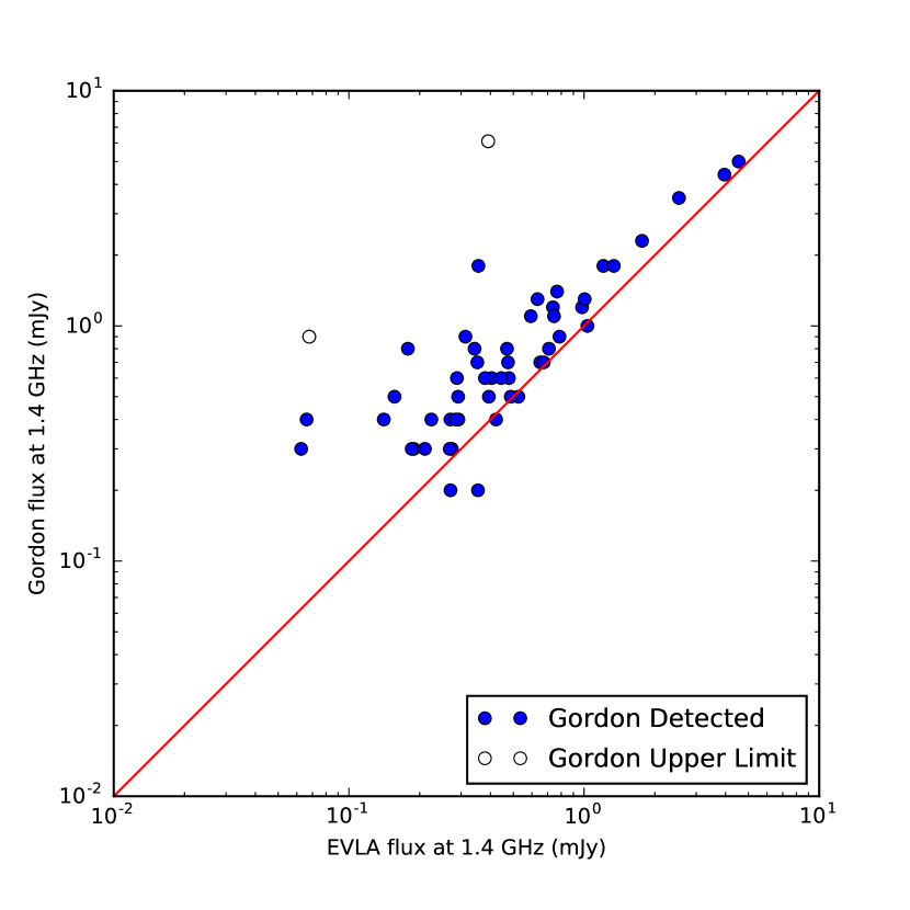
Figure 17: A comparison between our measured 1.4 GHz flux densities in the forced photometry catalog and those reported by G99. The open circles show sources that G99 reported as detections at 5 GHz, but only upper limits at 1.4 GHz. The points are plotted at the upper limit values.

3.1.1 Comparison to Previous M33 Radio Detections of SNRs

As noted in the Introduction, the last detailed radio study of SNRs in M33 was carried out by G99, who reported the radio detection of 53 out of 98 optically-identified SNR candidates that were known at the time. Of these 53 objects, 52 are in the region covered by our radio survey. All of these are detected at 3$\sigma$ or greater in our forced photometry catalog. As shown in Figure 17, there is a fairly good correlation between the flux densities we measure at 1.4 GHz (by constructing a weighted average of our two 1.4 GHz bands) and those measured by G99. The G99 flux densities tend to be higher, and in a few cases considerably higher. Many of the objects that are higher were identified by L10 as likely to be associated H II emission rather than emission from the SNR (or the SNR only). But the median of the ratio of the flux densities they measured is only 50% higher than those we measure suggesting that we and they are identifying the same radio sources as SNRs, but with differing amounts of contamination by thermal emission.

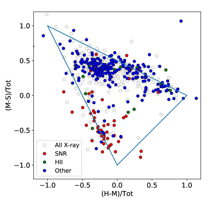
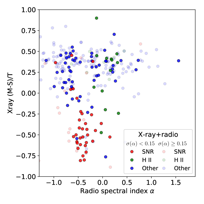
Figure 18: Left: Hardness ratio diagram of X-ray sources from Tüllmann et al. (2011) that are detected via forced photometry in our radio map. Sources identified with SNRs are shown in red, and H II sources in green. Open circles are X-ray sources that fall below the $3\sigma$ radio detection threshold. Right: X-ray hardness for the sources as reflected by the $(M-S)/T$ ratio as a function radio spectral index. Sources with noisy spectral indices are shown as pale symbols.

3.2 X-ray Sources Detected in Our Radio Survey

The Tüllmann et al. (2011) catalog of X-ray sources in M33 contains 662 X-ray sources, the vast majority of which are due to background sources (galaxies and AGN). We detect radio emission at the position of 319 of these sources at 3$\sigma$ or greater via forced photometry. Of these, 55 are positionally coincident with SNRs and 25 with H II regions observed by Lin et al. (2017). As shown in the X-ray hardness ratio diagram in the left panel of Figure 18, most of the X-ray sources we detect lie in the region of the diagram where background sources and X-ray binaries are expected to fall. As expected, the sources identified with SNRs mostly have soft X-ray spectra. The X-ray sources associated with H II regions are not concentrated in a particular region of the diagram, suggesting a mix of source types (X-ray binaries in M33, unrecognized SNRs, and background objects). The right hand panel of the figure shows X-ray hardness ratios as function of the radio spectral index. The SNRs form a well defined region in the diagram; this suggests that one might be able to identify SNRs directly from such a diagram with sufficiently sensitive X-ray and radio observations, even without a prior optical identification.

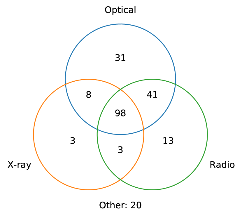
Figure 19: A Venn diagram showing the number of SNRs that have been detected in various wavelength bands and combinations thereof. For this comparison, the optical SNRs must have a spectrum showing that the ratio [S II]:H$\alpha$ $\geq$ 0.4. Optical SNR candidates for which no spectra have been obtained or for which spectra failed to confirm a high ratio could still align with a radio or X-ray source. These account for the sources shown as X-ray, radio, or radio–X-ray only. There are an additional 20 optical SNR candidates from imaging surveys that have no confirming optical spectra and no radio or X-ray emission. See text section 3.3 for full details.

3.3 Multi-wavelength Comparisons

A Venn diagram showing the number of objects detected in the various wavelength bands is shown in Figure 19. To be counted as a confirmed optical SNR, we require not only that a nebula was suggested either by L10 or LL14 as a candidate based on interference filter imagery, but that a spectrum exists that confirms the [S II]:H$\alpha$ ratio is at least 0.4, the conventional criterion for declaring that an emission nebula is a valid optical SNR candidate. There are 98 emission nebulae satisfying this criterion, that also show up as positive detections in our radio forced-photometry catalog, and that have been detected at 3$\sigma$ or greater with either Chandra or XMM-Newton. Additionally, there are 31 optical SNRs with spectral confirmations but without detected X-ray or radio counterparts, 41 that have a radio counterpart but no X-ray, and 8 objects with optical–X-ray detections but no radio counterpart.

The small numbers in the non-optical parts of the diagram deserve specific discussion. The location of an individual object in the Venn diagram depends on many factors, not the least of which is our application of the optical spectral confirmation criterion above and beyond the imaging candidate status. There are optical SNR candidates that were identified from imaging but have no optical spectra, and there are optical candidates for which the spectra obtained showed [S II]:H$\alpha$ ratios somewhat below 0.4. The objects that lie in the X-ray (3), Radio (13), and radio–X-ray (3) portions of the Venn diagram align with some of these objects.

For the 13 “radio-only” objects, five do not have spectra, two were too contaminated for accurate spectral measurements, and six have spectra with derived [S II]:H$\alpha$ ratios below 0.4. Three of these objects had [S II]:H$\alpha$ ratios between 0.36 and 0.39, and the other three were near 0.25. However, for fainter objects or objects with nearby H II contamination, even the spectrally-derived ratios can have significant errors bars. If the background H$\alpha$ is even slightly under-subtracted in the spectra, the derived [S II]:H$\alpha$ ratio can be artificially lowered. The presence of associated radio emission for these eight objects significantly enhances the probability that these nebulae are SNRs.

Of the three ‘X-ray-only’ objects, one has no optical spectrum, one is too contaminated to make a good measurement, and one has a spectrum with a [S II]:H$\alpha$ ratio of 0.27, significantly below the threshold (LL14-008). The presence of an X-ray source at the optical position strengthens these as possible SNRs as well.

The three objects shown as having both radio and X-ray emission would already seem to be strong candidates. All three have optical spectra with derived [S II]:H$\alpha$ ratios of 0.37 (L10-035), 0.33 (L10-040), and 0.37 (LL14-005). Again, slight H$\alpha$ background subtraction problems could have caused these to fall below our normal threshold ratio, so these are quite likely SNRs.

There are 20 emission nebulae that, other than their original selection as nebulae with enhanced [S II]:H$\alpha$ ratios from imaging, have no additional supporting information to suggest that they are SNRs, and thus do not appear in this diagram. This does not necessarily mean that they are not SNRs since some objects have not been observed spectroscopically, and one other was simply outside of the region surveyed with the JVLA. Fourteen of the 20 have spectra that show ratios below the normal threshold, so without further corroboration the majority of these are probably not SNRs.

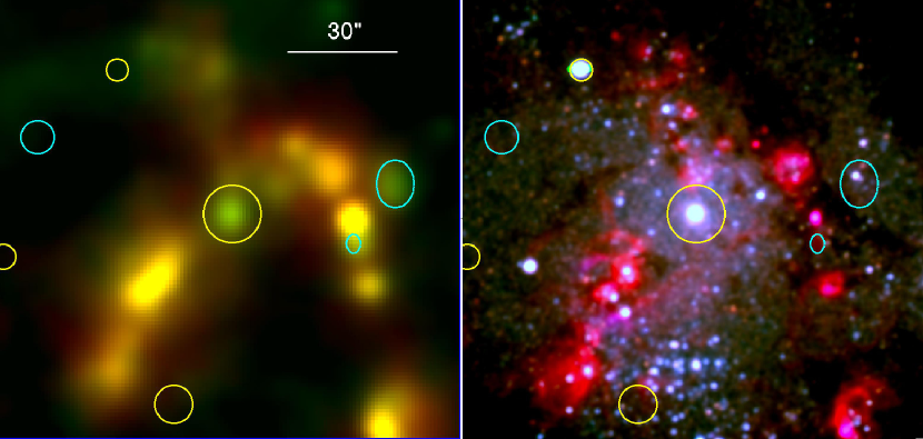
Figure 20: A view of the 2′ region near the center of M33. The same data shown in Fig. 2 have been rescaled to just highlight the nuclear region. A steep-spectrum (green) source in the left panel corresponds to the bright optical source in the nucleus; numerous nearby H II regions are bright radio sources as well. Yellow region overlays indicate X-ray source positions from Long et al. (2010) and the cyan regions indicate optical SNR detections nearby.

4 Discussion

4.1 The Nuclear Source and other X-ray binaries

With an X-ray luminosity of $\sim$$\rm 10^{39}\rm\>\>{\rm ergs\>s^{-1}}$, M33 X-8, the source coincident with the the nucleus of M33, is one of the brightest persistent X-ray sources in the Local Group (Long et al., 1981). The nuclear star cluster is compact but otherwise unprepossessing optically; its spectrum can be modeled in terms of two bursts of star formation, one with an age of 40 Myr involving stars with a total mass of 9000$\>M_{\sun}$, and another of age 1 Gyr with a mass of 76,000 $\>M_{\sun}$(Long et al., 2002). If a black hole exists at the center of the cluster it must have a mass $<$1500$\>M_{\sun}$(Gebhardt et al., 2001). It has been suggested (although not confirmed) that the nuclear source has a period of 109 days (Dubus et al., 1997). Taken together, these observations imply the source is not an AGN but is instead an $\sim$10$\>M_{\sun}$ X-ray binary radiating near the Eddington limit (see, e.g. Foschini et al., 2004; Middleton et al., 2011).

As shown in Figure 20, a non-thermal radio source, W19-0683, is coincident with the nucleus. The spectral index is $-0.39\pm 0.11$ and the flux at 1.4 GHz is $0.61\pm 0.04$ mJy. The radio source is extended, with a ratio of peak to integrated flux density of 0.35 (compared with unity for a point source), and a nominal major axis of 18″, or 70 pc. In the forced photometry catalog, where source T11-318 corresponds to the nuclear source, the 1.4 GHz flux is similar, $0.60\pm 0.04$ mJy, with a slightly steeper spectral index of $-0.68\pm 0.17$. (The spectral indices in the main catalog and the X-ray catalog are consistent, differing by $1.4\sigma$.) The nuclear source was also observed by G99 who reported a consistent flux density ($0.6\pm 0.2$ mJy at 1.4 GHz) and spectral index ($-0.8\pm 0.3$). For comparison, SgrA* in our Galaxy, which arises from the accretion disk of a $4\times 10^{6}$$\>M_{\sun}$ black hole (BH), is a 0.7 Jy source at 1.4 GHz, corresponding to $\sim 0.07$ mJy at the distance of M33, and has a spectral index of $-0.3$ (Duschl & Lesch, 1994).

Whether M33 X-8 is very low mass BH at the nucleus of M33 or simply, as is generally thought, a BH binary, the existence of radio emission is not surprising, given that BH systems on all mass scales produce radio emission (see, e.g., Plotkin et al., 2012). The 1.4 GHz radio luminosity of M33 X-8 is about $6.7\times 10^{32}\rm\>\>{\rm ergs\>s^{-1}}$, less than $\rm 10^{-6}\rm\>t$he X-ray luminosity. Exactly how to fit M33 X-8 into the zoo of BH binaries remains unclear. It has properties that resemble a microquasar trapped in the so-called high soft state, where disk accretion is near the Eddington rate (Long et al., 2002; Foschini et al., 2004). Most microquasars, however, exhibit major outburst events, and M33 X-8 has not been seen to vary appreciably. During the rise to X-ray maximum, microquasars show active radio jet emission (with flat spectral indices) and hard X-ray spectra. At outburst maximum, however, the X-ray spectra transition to something similar to that of M33 X-8 and the radio spectral indices steepen. The idea is that active jet generation has ceased (or ebbed at least), and the residual emission arises from the interaction with the surrounding medium (Fender et al., 2004).

Because of its X-ray luminosity and the fact that the luminosity is persistent, M33 X-8 has also been characterized as an ultraluminous X-ray source (ULX). It is at the low luminosity end of sources classified as ULXs that also have X-ray spectra fit in terms of steady state accretion onto a massive BH. Other ULXs in this state observed at radio wavelengths have spectral indices characteristic of optically thin synchrotron emission. The radio emission for a number of the nearest ULXs (and microquasars) has been resolved, and appears to arise from a jet interaction with the surrounding ISM (Pakull & Mirioni, 2003). The typical sizes of the resolved bubbles around these sources are 100-300 pc. At the resolution of our observations (about 20 pc), the bulk of the radio emission in M33 X-8 appears point-like, although, as mentioned above, the source is extended at the $\sim$70 pc level. Thus, source extent does not rule out the jet-interaction scenario in M33 X-8. The prototypical high-mass X-ray binary Cygnus X-1 is surrounded by a 5 pc diameter radio ring that appears to have been inflated by a jet from the central source (Gallo et al., 2005). Clearly, sensitive, higher resolution radio observations are needed to clarify the situation for M33 X-8.

In addition to detecting a nuclear radio source, radio sources were also detected at the positions of several other known X-ray binaries in M33. Among these is a source with a 1.4 GHz flux density (in the forced photometry catalog) of $0.63\pm 0.02$ mJy at the position of M33 X-7, the well-studied eclipsing BH binary, comprised of a 16$\>M_{\sun}$ BH orbiting a 70$\>M_{\sun}$ O-star every 3.45 days (Orosz et al., 2007). However, the spectral index of this source is $0.08\pm 0.02$ and the H$\alpha$ surface brightness at this position is high, about $3.4\times 10^{-15}\rm\>ergs~{}cm^{-2}s^{-1}arcsec^{-2}$, suggesting that most if not all of the radio emission arises from H II regions along the line of sight. A similar situation obtains for M33 X-4, another bright X-ray source thought to be an X-ray binary (Grimm et al., 2007), where the forced photometry 1.4 GHz flux density is $0.17\pm 0.01$ mJy, but the apparent spectral index is $+0.3\pm 0.1$. This source is also located along a line of sight with considerable H$\alpha$ flux, $1.1\times 10^{-15}\rm\>ergs~{}cm^{-2}~{}s^{-1}~{}arcsec^{-2}$. Higher resolution observations are required to determine whether either of these sources has any intrinsic radio emission.

4.2 The M33 SNR Sample: Models vs. Data

Our large sample of SNRs with both radio and X-ray luminosities enables some useful comparisons to models for SNR radio emission. Sarbadhicary et al. (2017) describes a relatively simple analytical model for the radio luminosities of SNRs as a function of their radius, evolutionary phase, ISM density, explosion energy, etc. According to equation (A12) in Sarbadhicary et al. (2017), the radio luminosity density $L_{\nu}$ at 1.4 GHz is given by:

$$L_{1.4}={} \mbox{\rm$2.2\times 10^{24}\rm\>ergs~{}s^{-1}Hz^{-1}$}\left(\frac{R}{10\,\mathrm{pc}}\right)^{3}$$ (1)

$$\left(\frac{\epsilon_{e}}{10^{-2}}\right)\left(\frac{\epsilon^{u}_{b}}{10^{-2}}\right)^{0.8}\left(\frac{v_{s}}{500~{}\mathrm{km~{}s}^{-1}}\right)^{3.6}$$

where $R$ is the shock radius, $v_{s}$ is the shock velocity and $\epsilon_{e}$ and $\epsilon^{u}_{b}$ are the fractions of the post shock energy density $\rho v_{s}^{2}$ converted into relativistic electrons and the amplified upstream magnetic field in a diffuse acceleration model, respectively.

If this model were correct, and if all other factors except the shock velocity were the same, $L_{1.4}$ would be a strong function of $v_{s}$. Indeed, a factor of two difference in shock velocity would correspond to a factor of 12 difference in $L_{1.4}$. The radio luminosity also increases in proportion to the SNR volume, $L_{1.4}\sim R^{3}$. As a result, during the SNR free expansion phase, when the shock velocity is constant, the radio luminosity increases rapidly as $R^{3}\sim t^{3}$. The radio luminosity peaks at the beginning of the Sedov phase, declines through the adiabatic expansion phase as the shock slows, and finally decreases rapidly in the radiative phase as $v_{s}$ drops off and the SNR expansion slows.

Sarbadhicary et al. (2017) assume that $\epsilon_{e}$ is constant with time, citing Soderberg et al. (2005) and Chevalier & Fransson (2006). However, $\epsilon^{u}_{b}$ is not a constant in this equation but depends on the magnetic field, shock velocity, and other parameters. Following the discussion in their appendix, the definition of $\epsilon^{u}_{b}$ is:

$$\epsilon^{u}_{b}=\frac{B^{2}/8\pi}{\rho v^{2}_{s}}$$ (2)

Citing Bell (2004), Sarbadhicary et al. (2017) argue that at high Alfvén Mach number ($M_{A}$), magnetic amplification saturates at a value given by:

$$\frac{B^{2}}{8\pi}\sim\frac{1}{2}\frac{v_{s}}{c}\xi_{cr}\rho v^{2}_{s}$$ (3)

where $\xi_{cr}$ is the fraction of shock energy that goes into relativistic particle acceleration (including electrons and ions). They then assume $\xi_{cr}$ is a constant value of 0.1 for high Alfvén Mach numbers but declines for smaller $M_{A}$:

$$\xi_{cr}=\begin{cases}0.1&\text{when }M_{A}>30\quad,\\ 10^{-2}\left(0.15\,M_{A}+6\right)&\text{when }M_{A}<30\quad.\end{cases}$$ (4)

Here $M_{A}<30$ is an approximate limit – $\xi_{cr}$ increases in proportion to $M_{A}$ until it saturates at a value $\xi_{cr}=0.1$.

The final equation that Sarbadhicary et al. (2017) use for $\epsilon^{u}_{b}$ is

$$\epsilon^{u}_{b}=\frac{\xi_{cr}}{2}\left(\frac{v_{s}}{c}+\frac{1}{M_{A}}\right)$$ (5)

That makes a transition from values that are proportional to the shock velocity $v_{s}$ (at high $M_{A}$ values) to values that are proportional to $1/M_{A}$, meaning $\epsilon^{u}_{b}$ scales as $1/v_{s}$, at lower shock velocities. Coincidentally, Figure A1 in Sarbadhicary et al. (2017) shows that the transition between these scalings occurs close to the beginning of the Sedov phase of evolution. In the example they show, the value of $\epsilon^{u}_{b}$ varies by only a factor of three from the initial SN explosion to an age of $2\times 10^{4}\rm\>yr$; given the modest dependence of $L_{1.4}$ on $\epsilon^{u}_{b}$ this implies that $\epsilon^{u}_{b}$ contributes only a factor of $\sim$2 to the variation in $L_{1.4}$ over a SNR lifetime. That is why the treatment of $\epsilon^{u}_{b}$ as a constant in equation (1) is approximately correct.

The $\epsilon^{u}_{b}$ term also introduces dependencies on the density $n_{H}$ and magnetic field $B_{0}$ in the ISM. And the magnetic field itself depends on the ISM density since it is coupled to the ISM state. Equation (A4) of Sarbadhicary et al. (2017) can be rewritten to give the ISM magnetic field as

$$B_{0}=9\,\mu\mathrm{G}\,n_{H}^{0.47}\quad,$$ (6)

where $n_{H}$ is the ISM hydrogen number density.

To see what this model for the radio emission means, it is useful to recall the Sedov equations:

$$R=5.2\,\mathrm{pc}\left(\frac{E_{51}}{n_{H}}\right)^{1/5}\left(\frac{t}{1000\,\mathrm{yrs}}\right)^{2/5}$$ (7)

$$v_{s} =2000\>{\rm km\>s^{-1}}\left(\frac{E_{51}}{n_{H}}\right)^{1/5}\left(\frac{t}{1000\,\mathrm{yrs}}\right)^{-3/5}$$ (8a)

$$=\frac{2}{5}\frac{R}{t}$$ (8b)

$$=3900\>{\rm km\>s^{-1}}\frac{R/10\,\mathrm{pc}}{t/1000\,\mathrm{yr}}$$ (8c)

In the Sedov phase, the radio luminosity density $L_{1.4}$ from equation (1) can be expressed as a function of $t$:

$$L_{1.4}={} \mbox{\rm$4.8\times 10^{25}\rm\>ergs~{}s^{-1}Hz^{-1}$}\left(\frac{t}{1000\,\mathrm{yr}}\right)^{-0.96}$$ (9)

$$\left(\frac{\epsilon_{e}}{10^{-2}}\right)\left(\frac{\epsilon^{u}_{b}}{10^{-2}}\right)^{0.8}\left(\frac{E_{51}}{n_{H}}\right)^{1.32}\quad.$$

For this relationship and assuming $\epsilon^{u}_{b}$ is approximately constant, then according to Sarbadhicary et al. (2017), we should expect $L_{1.4}\propto t^{-0.96}$. A SNR in the Sedov phase should be brightest when it enters the Sedov phase and should decline linearly with time (ignoring the variation in $\epsilon^{u}_{b}$).

The radio luminosity can also be expressed as a function of $R$:

$$L_{1.4}={} \mbox{\rm$1.0\times 10^{25}\rm\>ergs~{}s^{-1}Hz^{-1}$}\left(\frac{R}{10\,\mathrm{pc}}\right)^{-2.4}$$ (10)

$$\left(\frac{\epsilon_{e}}{10^{-2}}\right)\left(\frac{\epsilon^{u}_{b}}{10^{-2}}\right)^{0.8}\left(\frac{E_{51}}{n_{H}}\right)^{-9/5}\quad.$$

Thus we expect small diameter SNRs to be significantly brighter, all other things being the same ($L_{1.4}\propto R^{-2.4}$). Clearly we do not see our observations reflecting this dependence (cf. Fig. 15).

On the other hand, this relationship does allow for significant variations in the radio luminosity at a specific diameter if the ratio $E_{51}/n_{H}$ varies significantly. A SNR with an explosion energy of $10^{51}\,\mathrm{erg}$ expanding into an ISM with density 1 cm^-3 would be 63 (4000) times brighter than one expanding into an ISM with density 0.1 (0.001) cm^-3, assuming both are in the Sedov phase. (See also Asvarov, 2006, who reached a similar conclusion about radio luminosity variations associated with variations in $E_{51}/n_{H}$ from models made with slightly different assumptions.)

If the variations in radio luminosity are primarily due to variations in $n_{H}$, then we would expect that to have consequences at X-ray wavelengths, where emission arises from the same shock that powers the radio emission. Simply put, SNRs expanding into a dense ISM are brighter at the same diameter in soft X-rays than those expanding into a tenuous one, so we would expect radio-bright SNRs to also be X-ray bright and vice versa. Berkhuijsen (1986) argued that a correlation of this type does exist using a collection of Galactic and extragalactic SNRs; here we discuss the specific case of M33.

The X-ray luminosity in the Sedov phase has a complex dependence on the physics involved (e.g., non-equilibrium ionization, electron conduction, etc.). However, White & Long (1991) give a simple approximation based on the observation that the X-ray emissivity function $\Lambda_{x}(T)$ is constant to within 50% over a wide range of temperature (Hamilton et al., 1983). From equation (21) in White & Long (1991):

$$L_{x}={} \mbox{\rm$3.0\times 10^{37}\rm\>ergs~{}s^{-1}$}\left(\frac{R}{10\,\mathrm{pc}}\right)^{3}n_{H}^{2}$$ (11)

$$\left(\frac{\Lambda_{x}}{\mbox{\rm$1\times 10^{-22}\rm\>erg~{}cm^{3}s^{-1}$}}\right)\quad,$$

where we set the contribution of evaporating clouds to zero and are using an ISM density $n=\rho/m_{H}=0.75\,n_{H}$. Combining equations (10) and (11), we can calculate the ratio of the radio luminosity $L_{R}=\nu L_{\nu}$ to the X-ray luminosity:

$$\frac{L_{R}}{L_{x}}={} \mbox{\rm$4.6\times 10^{-4}\rm\>$}\left(\frac{R}{10\,\mathrm{pc}}\right)^{-5.4}n_{H}^{-1/5}E_{51}^{-9/5}$$ (12)

$$\left(\frac{\Lambda_{x}}{10^{-22}}\right)^{-1}\left(\frac{\epsilon_{e}}{10^{-2}}\right)\left(\frac{\epsilon^{u}_{b}}{10^{-2}}\right)^{0.8}\quad.$$

Note that this decreases rapidly with radius but depends very weakly on the ISM density. It predicts that large-diameter SNRs should have much lower $L_{R}/L_{x}$ ratios, regardless of the local ISM density (which may vary widely among remnants).

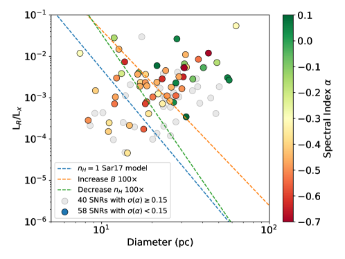
Figure 21: The ratio of the radio luminosity $\nu L_{\nu}$ at 1.4 GHz to the X-ray luminosity as a function of diameter $D$ for SNRs in M33. The Sarbadhicary et al. (2017) radio luminosity model predicts that in the adiabatic expansion (Sedov) phase, this ratio should decline rapidly with diameter. The blue dashed line is for nominal model parameters with $n_{H}=1\,\mathrm{cm}^{-3}$. While the model predictions depend on the ISM density and magnetic field, even changes by a factor of 100 (red and green lines) do not affect the conclusion that the observed variation of $L_{R}/L_{x}$ with diameter is much flatter than the predictions. The SNRs that have well-determined spectral indices have symbols color-coded by $\alpha$; objects that are too faint to have an accurate $\alpha$ (including those in regions that lack 5 GHz data) are shown in gray.

This appears to be in sharp conflict with the observations (Fig. 21). There is a wide range of radio-to-X-ray ratios at all SNR diameters, and there is no indication of a marked decline for larger SNRs. The dashed lines show the model prediction from equation (12). We have included in the model calculation the additional dependence on $B$ and $n_{H}$ that comes through the $\epsilon^{u}_{b}$ factor by using equation (5) rather than assuming $\epsilon^{u}_{b}$ is constant. But even large changes in the ISM density and the $B$ field scaling in equation (6) have little effect on the general trend. Moreover, Elwood et al. (2019) found that the scatter in $n_{H}$ for SNRs in M31 and M33 is relatively small ($\log n_{H}\sim-1.35\pm 0.7$), which makes explanations that rely on a wide variation in the ISM density problematic. The predicted $L_{R}/L_{x}$ ratios from the Sarbadhicary et al. (2017) model are too low at $D\sim 30\,\mathrm{pc}$ by one to two orders of magnitude compared with the observations, even using extreme parameter values.

We have considered several possible explanations for the discrepancy in the $L_{R}/L_{x}$ ratio predictions compared with the observations. Our calculation assumes that the SNR is in the Sedov phase. That is likely to be a good assumption since the radio and X-ray luminosities both decline dramatically at the onset of the late radiative phase (Asvarov, 2006), while the early free-expansion phase is short ($\sim 10^{2}$ yr) and can only be relevant for small-diameter remnants (Elwood et al., 2019).

Another possible explanation is that the forced photometry SNR radio fluxes are contaminated by emission from nearby H II regions, leading to elevated values of $L_{R}/L_{x}$. To test this hypothesis, Figure 21 shows (via the symbol colors) the spectral indices of the SNRs. If H II contamination were important, all the large diameter SNRs would have the thermal spectral indices typical of H II regions, $\alpha\sim 0$, rather than the non-thermal $\alpha\sim-0.5$ indices observed for most SNRs. While there is an indication that some of the largest diameter SNRs have thermal contamination, there are also large diameter SNRs with non-thermal spectra. Care is required to account for the overestimated radio luminosities for SNRs embedded in H II regions, but that effect cannot explain the large $L_{R}/L_{x}$ ratios in M33.

As shown In Figure 12, the luminosity function for the SNRs we detect can be represented as a power law, as was pointed out by Chomiuk & Wilcots (2009) for M33 (and a number of other galaxies) based on earlier data. Chomiuk & Wilcots (2009) sought to interpret this fact in terms of a model that was similar to that of Sarbadhicary et al. (2017). While it may well be true that the radio luminosity function of SNRs can be represented as a power law, our analysis makes it clear that a physical connection between the observations and the theory is lacking.

Although we have chosen to focus on the specific model for radio emission in SNRs described by Sarbadhicary et al. (2017), this model embodies the same elements as most other models of radio emission in SNRs. We conclude that the $L_{R}/L_{x}$ ratio is a strong diagnostic for testing models of radio emission from SNRs in the presence of ISM density variations. Apparently current models still have significant shortcomings when confronted by the radio and X-ray observations.

4.3 Comparison to Radio Studies of Other Galaxies

4.3.1 Large Magellanic Cloud

As a result primarily of their proximity (and low Galactic extinction), more is known about the SNRs in the Magellanic Clouds than in any other galaxies. As recently summarized by Bozzetto et al. (2017), there are now 59 confirmed SNRs in the Large Magellanic Cloud (LMC), of which 42 have radio fluxes at 1 GHz and 51 have X-ray spectra (Maggi et al., 2016). The existence of high quality X-ray spectra (not possible to obtain for most of the SNRs in M33) has allowed most of the SNRs to be typed as the products of core-collapse or Type Ia explosions. There are also another 15 candidates, most of which are larger objects with typical diameters of 100 pc or more. The median diameter for the SNRs in the LMC is about 40 pc, very similar to that in M33, but unlike M33, the LMC does have several SNRs known to have ages less than a few thousand years. As noted by Long et al. (2010) and more recently by Maggi et al. (2016), the LMC has more very luminous X-ray SNRs than M33. There is a rough correlation between radio and X-ray brightness that is particular evident in the subsample of core-collapse remnants, where ejecta interactions are still important (Bozzetto et al., 2017).

In the LMC, the radio data suggest that the radio spectral index of SNRs flattens with time and diameter, especially among the SNRs associated with core-collapse SNe, with younger 10 pc diameter SNR having a spectral index of about $-0.6$ pc and older 40 pc objects having spectral indices around $-0.5$ (Bozzetto et al., 2017). The correlation is considerably less apparent in the Galactic sample, but as Bozzetto et al. (2017) point out, one would expect a sample from an external galaxy to be cleaner as a result of the fact that all of the SNRs are at the same distance and, as a result of this, have similar apparent sizes.

Firmly establishing a correlation between spectral slope and other properties of a SNR sample is clearly important, since it suggests that the structure of the shock front and/or the nature of the physical processes that generate radio emission are changing with time or with shock velocity. Indeed, various suggestions for what might be changing have been proposed, based either on earlier hints at spectral slope changes, or by noting that specific types of SNRs (such as those interacting with molecular clouds) had flatter spectral indices than the general populations of SNRs (see, e.g. Bell et al., 2011; Urošević, 2014).

We do not see a similar correlation in M33 (Fig. 15b). We do not have an explanation for the difference. Although the properties of the LMC and M33 certainly differ in terms of star formation history and ISM properties (including magnetic field strengths and cosmic ray densities), it is not clear why any of these properties would lead to a different trend. From an observational perspective, if an object has a flux of 1 mJy at 1.4 GHz it will have a flux of 0.53 or 0.47 mJy at 5 GHz, depending on whether the spectral index is $-0.5$ or $-0.6$, respectively, so obtaining accurate spectral slopes requires accurate flux measurements from interferometric observations. In the case of our JVLA observations, we have taken a lot of care to match beam sizes and to extract accurate fluxes, but even so these are technically challenging observations. The radio spectral indices compiled by Bozzetto et al. (2017) included measurements made by various investigators with different instrumental setups. As result, we believe it is very important that more attempts be made to establish whether the correlation seen by Bozzetto et al. (2017) can be replicated with either newer observations of the LMC with a single observational setup or in other galaxies.

4.3.2 M31

With a limiting sensitivity of 20 $\mu$Jy ($4\sigma$) or $\nu L_{\nu}$ = $2.2\times 10^{31}\rm\>\>{\rm ergs\>s^{-1}}$, and a resolution of 5.9″ or 23.6 pc at a distance of 817 kpc, this JVLA survey of M33 is the deepest radio survey of any extragalactic spiral galaxy. In contrast, its neighbor M31 has not been surveyed to anything approaching this depth, in part, of course, due to its large angular size. Galvin & Filipovic (2014) used archival data from the VLA to construct a catalog of radio sources in M31, but their 1.4 GHz catalog has a limiting sensitivity of only $\sim$2 mJy and contains some 916 sources. Of these, just 98 have spectral indices, most of which are steep and characteristic of either background AGN or SNRs. Of the 156 optical nebulae identified as SNR candidates in M31 by Lee & Lee (2014b), only 13 lie within 5″ of sources in the radio catalog, a much lower fraction than is observed in M33. Presumably this is a result of the much lower sensitivity of the M31 radio catalog.

4.3.3 M83

Long et al. (2014) carried out a deep Chandra observation of M83 supplemented by radio observations with ATCA at 5 and 9 GHz. The radio catalog consisted of 102 sources, the faintest of which is $\sim$50 $\mu$Jy  at 5 GHz, corresponding to $\nu L_{\nu}$ of $6.3\times 10^{33}\rm\>\>{\rm ergs\>s^{-1}}$ at the assumed 4.6 Mpc distance of M83. Many of the radio sources were in the spiral arms of M83. Of the 102 sources, 21 were identified with one of the 225 optical SNR candidates known in M83 at the time (Blair et al., 2012). Another 15 were identified with other Chandra X-ray sources; some of these may be SNRs but most are likely to be background sources in the field or H II regions in which an X-ray binary is embedded.

4.3.4 NGC 7793

Galvin et al. (2014) used archival ATCA data on the southern Sculptor group galaxy NGC 7793 obtained at 1.4, 5 and 9 GHz to create a catalog of 76 sources brighter than 11 $\mu$Jy per beam (3 $\sigma$) or $\nu L_{\nu}$ = $1.3\times 10^{33}\rm\>\>{\rm ergs\>s^{-1}}$ at 5 GHz, using an assumed distance of 3.9 Mpc. They classified 57 sources; 37 are most likely H II regions. The microquasar known as NGC 7793–S26 was also detected. They claimed 14 SNR identifications, but they applied an unusual definition of a SNR candidate as a radio source with a steep radio spectral index associated with an X-ray source. Many such sources in the M33 catalog are clearly background AGN, and so this way of identifying SNR candidates is fraught with concern. An earlier paper by Pannuti et al. (2002) listed five radio SNR candidates in NGC 7793 identified using the criterion of a nonthermal radio source aligned with optical H$\alpha$ emission, as used by Lacey & Duric (2001), but again, this is suspect without the use of the [S II]:H$\alpha$ criterion. Of the 28 optical SNR candidates in the survey by Blair & Long (1997), only two objects had radio counterparts in Pannuti et al. (2002), one of which was the aforementioned NGC 7793–S26. Galvin et al. (2014) found only five of the ATCA sources that aligned with any SNR candidate from the earlier lists. Clearly very few radio SNRs have been detected in NGC 7793.

4.3.5 Efficacy of SNR identification using radio emission

Most extragalactic SNRs and SNR candidates have been identified optically based on [S II]:H$\alpha$ emission line ratios. However, some attempts have been made to identify SNRs in other galaxies on the basis of their radio properties, usually coupled with more limited optical data. For example, Lacey & Duric (2001) identified 35 radio-selected SNRs/SNR candidates in NGC6946 on the basis of their non-thermal radio spectral indices and associated H$\alpha$ emission. These SNRs were concentrated in the spiral arms of NGC 6946. They compared this sample to one obtained by Matonick & Fesen (1997) optically and found very little overlap between the two samples. The Matonick & Fesen (1997) sample was distributed in both arm and interarm regions of the galaxy and so Lacey & Duric (2001) argued that the fact that the samples were largely disjoint was a selection effect. Optical SNRs are simply difficult to pick out against the light of an H II region. Most SNe occur in star forming regions of a galaxy and hence most SNRs should exist in the spiral arms. Star forming regions are also the regions of a galaxy with the most H$\alpha$ emission and therefore the fact that optical SNRs are not concentrated there is prima facie evidence that they are being missed in optical surveys.

The general argument made by Lacey & Duric (2001) that there are portions of a galaxy where optical SNR detection is difficult has to be correct at some level, but it raises a number of questions, especially as many of the spectral index measurements in radio maps are not precisely determined and that, with current instrumentation, it has been difficult to obtain any confirming evidence that a radio SNR candidate in an external galaxy based on radio criteria alone is indeed a SNR. On the theoretical side, these questions include how important it is that after the first SN explodes in a star cluster, subsequent SNe will explode into the region evacuated by the first SN. On the observational side, one of the questions is at what H$\alpha$ surface brightness will what fraction of SNRs actually be missed, and how many background interlopers will be counted as SNRs. Unfortunately, there has very little systematic work to investigate any of these problems.

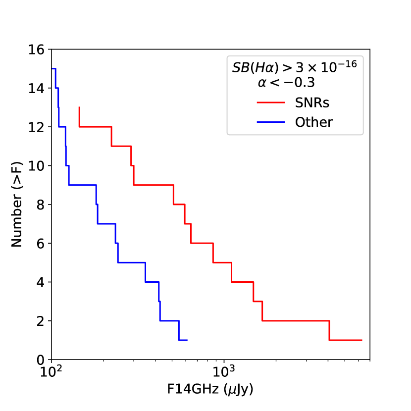
Figure 22: The number of sources with non-thermal spectral indices that lie on regions of high H$\alpha$ surface brightness. Radio sources identified with known SNRs and those that are not are plotted separately. The sample is restricted to objects with 5 GHz fluxes, so sources with $F(1.4\,\mathrm{GHz})>100\,\mu\mathrm{Jy}$ have well-determined spectral indices. The sources not known to be SNRs are almost certainly background objects. There are very few sources that are not SNRs above 0.6 mJy. That fact suggests that most radio sources identified in nearby galaxies as SNRs on the basis of a non-thermal radio spectral index in regions with H$\alpha$ emission are indeed good candidates, since most such surveys are not sensitive below 1 mJy.

We can use the observations of M33 to gain some insight into this. There are 284 non-thermal sources (with a spectral index of less than $-0.3$) in our survey that are brighter than 0.1 mJy and are in the region covered by our 5 GHz data. Essentially all of those sources have well-determined spectral indices. Of these, 28 lie at positions where the H$\alpha$ surface brightness exceeds $3\times 10^{-16}\rm\>\>{\rm ergs\>s^{-1}}~{}arcsec^{-2}$. Of these sources, 14 are known SNRs. However, most of the sources that are not known to be SNRs are quite faint. As shown in Figure 22, the number of interlopers drops quite rapidly as a function of the radio source brightness. At 200 $\mu$Jy, the number of interlopers and known SNRs is about the same, and at 600 $\mu$Jy essentially all of the interlopers have disappeared. At 200 $\mu$Jy  the typical spectral index error is 0.05 (1$\sigma$) in our survey, so confusion with H II regions is not a problem; nearly all of the non-SNRs are background sources. As our results are not very sensitive to the specific H$\alpha$ surface brightness limit chosen, and since the apparent distribution of fluxes of background sources does not depend on the distance to the foreground galaxy, this indicates that as long as a radio SNR candidate is relatively bright ($\gtrsim$ 0.5 mJy), radio SNR identifications should be fairly reliable, as Lacey & Duric (2001) suggested on the basis of their location.

4.4 Prospects for Future Radio Observations

The JVLA’s combination of high spatial resolution and wide frequency coverage provides an excellent tool for surveys of M33 and other nearby northern galaxies. Future observations that are higher resolution might enable algorithms that separate SNR emission from H II region emission using the morphology and spectral index of the radio flux. Higher angular resolution would also allow one to separate background objects from SNRs.

Improved algorithms for processing the very wide-band JVLA data could also enable more information to be extracted from our current data. Although we have put considerable effort in to development of new methods for analyzing multi-resolution radio images, we have deliberately degraded the resolution to generate images that are matched across the full frequency bandpass. One can imagine methods that might avoid this step.

Elsewhere, the LOFAR radio telescope is now being utilized for low frequency (0.15 GHz) surveys of the northern sky with a resolution of 6″ (Shimwell, T. W. et al., 2019). While this data alone will not produce accurate spectral indices from its 0.12–0.17 GHz bandpass, it should be readily combined with our similar-resolution, higher frequency JVLA observations. There are plans to do LOFAR observations of nearby galaxies including M33 to an rms sensitivity of 15 $\mu$Jy at 0.15 GHz (van Haarlem et al., 2013); for a SNR with a spectral index $-0.5$, that corresponds to an equivalent rms $\sim 5$ $\mu$Jy at 1.4 GHz, which is also well-matched to our survey.

The SKA pathfinder telescopes (ASKAP, MeerKAT) are located in the southern hemisphere and so are not directly relevant to studies of M33, but they should contribute interesting observations of other nearby galaxies. According to their specifications they will generate very deep images with noise comparable to or better than our JVLA data (Johnston et al., 2008; Norris et al., 2011, 2013). Their lower resolution of 10–15″ will make studies in the vicinity of H II regions more challenging, and their initial configurations have a more limited frequency range than the JVLA. Nonetheless, with a flood of high quality radio data on the horizon, we can expect dramatic advances in our understand of radio emission from SNRs over the next decade.

5 Summary and Conclusions

We have carried out a radio survey of M33 using the JVLA at 1.4 GHz and 5 GHz. After adjusting all of the various radio bands to a common angular resolution of 5.9″, our observations have a limiting sensitivity of 20 $\mu$Jy (4 $\sigma$). Using a new multi-resolution algorithm, we detect 2875 sources in the radio images. Additionally, we have extracted radio fluxes at the positions of several types of objects, notably SNRs and discrete X-ray sources in the Chandra X-ray survey of M33, in order to explore the radio properties of these objects. Our principal results are as follows:

• Most of the sources in the catalog can be categorized as (portions of) H II regions, SNRs, or background AGN. A few are aligned with X-ray binaries in M33 although some are buried in H II emission, making an assessment of intrinsic radio emission difficult. Catalog sources associated with H II regions have flat (thermal) spectral indices, whereas those associated with background galaxies and SNRs tend to have steep (non-thermal) spectral indices. Excluding the SNRs, the number and shape of the luminosity function of the steep spectrum sources is roughly consistent with that expected from radio surveys of high latitude fields.

• Of the 217 emission nebulae suggested to be SNRs in M33 as a result of optical interference imagery, we detect 141 in the catalog and 155 via forced photometry. As there is only one SNR outside the field of view of the radio maps we used for this analysis, we have detected (in forced photometry) 72% of the SNRs that we could have detected. Neither the radio luminosity nor the spectral index of SNRs in M33 is correlated with SNR diameter. There does appear to be a weak correlation between radio luminosity and H$\alpha$  luminosity, but the scatter is quite large. As discussed in Section 4.2, the radio luminosities of SNRs are not easily interpretable in terms of the current generation of models of radio synchrotron emission in SNRs.

• Of the 662 X-ray sources reported by Tüllmann et al. (2011), 320 are positionally coincident with sources in our radio catalog, and 319 are detected via forced photometry. Most of these have steep radio spectra and hard X-ray spectra. Most of these radio sources that are not SNRs are likely to be background AGN, seen in projection. One of the brightest radio sources in the survey is associated with the nuclear X-ray source X-8 in M33; the fact that there is radio emission is consistent with its identification as a microquasar, although the conclusion is not definitive.

Appendix A Multi-resolution source detection algorithm

This appendix describes a new multi-resolution algorithm that has been used to subtract the background from the radio images, to detect sources and identify regions with significant emission, and to measure the flux densities of those sources.

The traditional approach to measuring fluxes and source sizes from radio images is to fit elliptical Gaussians. That is the approach that was used for the FIRST survey (Becker et al., 1995; White et al., 1997) and for many other radio catalogs. However, Gaussian fits simply do not work well in fields as complex as our M33 JVLA images. The biggest problem is that in these deep, crowded images there may be many sources close together that must be simultaneously fitted. Also, many of the sources are extended with broad halos or tails around compact cores. Such objects are not well modeled by Gaussians. Even for sources that are roughly Gaussian, in crowded regions the Gaussian fits sometimes fail catastrophically, with a typical failure mode leading to source center positions that migrates to the edge of a shared boundary between adjacent islands. When that happens, the Gaussians are no longer distinct, and the fitted flux densities are poorly constrained. In principle, it might be possible to improve the Gaussian fitting procedures to handle these issues better, but it will be very difficult to produce good results for the full range of morphological variations in the radio sources.

Another approach is to integrate the map flux densities over the regions identified for each object. This has the major advantage that it does not depend on any assumptions about the source morphology. The disadvantage is that the uncertainty in the derived integrated fluxes is considerably greater than the uncertainties for Gaussian fits. This failing can be traced to the ability of the Gaussian fit to weight down pixels in island regions that are essentially empty, with pure noise, while giving higher weight to pixels where the object is detected. The unweighted sum of the island pixels weights each pixel equally and adds extra noise from the faint or empty regions in the island that may contribute little flux but still dominate the total noise.

We have developed a novel approach to this problem. We decompose the image into a stack of components of varying resolution using a median pyramid transform. The resulting stack has four levels (in this case), with the highest resolution (sharpest) level containing objects that are about the size of the PSF, the second level having objects that are twice that big, the 3rd level having objects that are $2^{2}=4$ times as big, etc. If the 4 levels are summed, the original image (including all sources and noise) is recovered exactly. But in any single level the noise is lower because higher frequency variations have been removed. The spatially varying background is also subtracted, making it easier to do photometry. The median pyramid is used to detect sources on a range of scales (which improves the detection of low surface brightness objects). Finally, the multi-resolution source detection maps are integrated over regions that adapt to include just the necessary pixels, reducing the noise while preserving the flux.

These steps are described in more detail below.

A.1 Median Pyramid

The median pyramid calculation begins with a median filter over a circular region of radius $R=8$ pixels (8″ for the full-resolution image). The median filtered image is the “smooth” channel, and the difference between the original image and the median-filtered image is the “sharp” channel. We also estimate the local rms noise as a function of position in the sharp channel by computing a second median filter, operating on the absolute value of the sharp channel and using an annular region with an inner radius of $R$ pixels and an outer radius of $2R$ pixels. The median absolute value is multiplied by 1.4826, a factor that converts the value to an equivalent Gaussian sigma when the noise is purely Gaussian. (This robust noise estimation approach is insensitive to outliers in the image.)

To create additional levels in the pyramid, the process is then repeated using the smooth image, with the radius of the filtering region expanded by a factor of two. This is iterated as many times as desired, with the filtering radius doubling at each new level. The choice of the number of levels determines the largest scale structure that remains in the image. For M33 we compute $L=4$ levels of the pyramid.

The median-filtered smooth channel has only faint residuals remaining at the positions of sources that are small compared with the filter area. We further reduce the contamination by sources in the smooth channel by doing a second filtering pass after removing pixels that are found to be larger than twice the local rms estimate. Those pixels are replaced by interpolating values from nearby pixels (using yet another median filter). Then the smooth channel is computed again. This single iteration of source rejection leads to very good removal of sources from the smooth channel.

We also improve the algorithm’s performance, which would be slow for higher levels of the pyramid when the filtering radius becomes large, by reducing the size of the smoothed image at each level by a factor of two in each dimension. We simply bin the smoothed image by averaging blocks of $2\times 2$ pixels. To compute the sharp image, we then re-expand the smoothed image back to the original size using bilinear interpolation. The result is a stack of smoothed images of decreasing size. With this modification, the iterated smoothing uses a median filter region that is the same size (in pixels) as used for the initial iteration. The effective radius is increased by a factor of two because the smoothed image was shrunk by that factor. The result is that the algorithm is actually faster for the higher levels of the pyramid.

When the median pyramid is complete, we are left with a stack of $L=4$ images ($L-1$ sharp images and the remaining smooth background image) along with $L-1$ local rms estimates for each sharp image. There are several adjustable parameters in the algorithm. The filter radius $R$ should be slightly larger than the PSF FWHM so that the first sharp images includes the point sources. The number of levels $L$, combined with $R$, determines the scale of the largest sources in the lowest resolution sharp image. Larger structures are in the final smooth image and are treated as background.

A.2 Source Detection

A single background-subtracted image can be constructed by summing the $L-1$ sharp channels. However, it is more effective to do source detection directly on the pyramid levels. At each level we use the FellWalker clump-finding algorithm (Berry, 2015) to identify islands of source emission. FellWalker identifies distinct peaks in the image and assigns nearby pixels to the nearest peak that is reachable by going uphill. It has parameters that prevent noise bumps from being included, that determine when two neighboring peaks have a significant valley between them, and that merge islands that are consistent with being noisy features of the same peak. The output of FellWalker is an island (or segmentation) map that divides the image into empty regions and contiguous regions at the locations of detected sources. We morphologically filter the FellWalker maps to eliminate islands that are smaller than expected given the resolution at that pyramid level.

There is one FellWalker island map for each level of the pyramid. We combine the independent island maps by merging islands that are detected in more than one level (which is a frequent occurrence). When necessary, islands that have multiple high-resolution peaks with overlapping low-resolution emission are split among the peaks using rules that attempt to maintain the morphological characteristics of the existing islands.

The merging process starts by creating a merged island map $M$ from the highest resolution image. The island numbers at each higher level are then updated using these rules:

1. Islands that do not overlap an existing island in $M$ get a new number larger than any existing island number.

2. Islands that overlap a single existing island in $M$ are assigned the same number as that island. This is the most common case (e.g., when a core-halo source is detected at several levels of the pyramid.)

3. Islands that overlap more than one existing island in $M$ are split and are assigned numbers chosen from among those islands:

   1. Pixels already assigned in $M$ to an island number retain their values.

   2. Unassigned pixels are assigned to the closest island using a distance metric that weights the Euclidean distance to the island center by the elliptical moments of the island shape in $M$.

   3. The extended islands are checked to ensure that they are contiguous. If non-contiguous regions are found, those pixels are reassigned to the second closest island.

4. After renumbering is complete, $M$ is updated by filling blank pixels with the corresponding values in the new level’s island map.

There are other algorithms that could be used for island splitting (case 3), but our approach is simple and has been found to produce reasonable results. The effect of our choice is to assign a pixel that is near two different islands to the island that reaches most closely toward that pixel, either because it is large or because it is elliptical and is extended in the direction of the pixel.

There are several advantages to this source detection approach. The detection of sources at each level is simplified because more extended background structures have already been subtracted. Sources that are extended with low surface brightnesses are much more easily recognized in the lower resolution levels of the pyramid. The island merging process provides a clear and simple approach for combining the source lists at different resolution levels. And finally, having a multi-resolution set of detection maps enables the computation of higher signal-to-noise flux density estimates for sources with complex morphologies that include sharp components embedded in broad halos. That algorithm is described below.

A.3 Extracting Fluxes

It is possible to combine the multi-resolution detection maps into a single map that assigns every pixel of the image to a particular source (or to the empty background). We use that map,for example, to display the locations of detected sources. In some applications it might be sufficient to sum the fluxes within islands in order to determine source brightnesses. In our images, however, that leads to relatively high noise for core-halo sources which have a sharp component surrounded by a lower surface brightness halo that can spread across many pixels.

To reduce the noise, we instead use the segmentation maps at each level of the image stack along with the image from that level of the stack. For each level we sum only the pixels that are detected in the island at that level. For a sharp core embedded in a broad halo, the sharp channel island (“level 0”) only includes the few pixels needed to cover the PSF. But the broad channel island (“level 1”) with the halo includes many more pixels. The flux for the object is the sum of the few pixels from level 0 plus the many pixels from level 1. It does not include all the level 0 pixels that are covered by the level 1 island. That decreases the noise in the sum by not adding in a bunch of empty pixels that contribute only noise. Moreover, the level 1 image is significantly smoothed, reducing the rms noise in that level. As a result, the pixels that are included over a large region for the smooth halo contribute significantly less noise to the sum.

Note also that sources that have only a sharp component (e.g., point sources) typically have islands that have no components at any of the lower resolutions. Omitting those pyramid levels from the sum also reduces the noise for compact sources.

The end result is that this approach effectively creates an adaptive set of weights for the image pixels that adjusts itself depending on the actual distribution of flux in the object.

A.4 Performance of the New Algorithm

Figure 23 shows a comparison between the simple (single level) island flux densities and our multi-resolution island flux densities (left panel), and a comparison of the fractional flux density errors $\sigma(F)/F$ (right panel). Sources are color-coded using the island flux. There is a bias in the measured flux densities, with the multi-resolution values being systematically lower for fainter sources. This is not unexpected since the multi-resolution islands are more tightly delineated, and some flux spills outside the summed regions. On the other hand, the right panel shows that the signal-to-noise in the measurements is about 20% better in the multi-resolution measurements. The fractional flux density errors are systematically lower for both bright and faint sources using the multi-resolution algorithm.

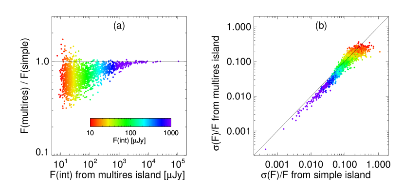
Figure 23: A comparison of the accuracy of flux densities determined using the multi-resolution island algorithm to flux densities computed using “simple” islands that are the same size at each resolution level. The left panel (a) shows the ratio of flux densities from the two methods. There is a systematic flux density underestimate by about $1\sigma$ for fainter sources due to the smaller island areas. The right panel (b) compares the fractional noise in the flux densities. The noise is about 20% smaller using the multi-resolution islands. The color of the points indicates the source brightness.

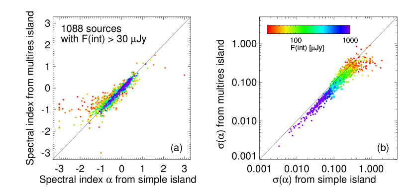
Figure 24: A comparison of the accuracy of spectral indices using the two island integration algorithms. The left panel (a) compares the spectral index $\alpha$ computed using “simple” islands (x-axis) to the value using the multi-resolution island. The agreement is excellent, particular for brighter sources. This plot includes only points with measurements at both 1.4 and 5 GHz and with flux densities greater than $30\,\mu\hbox{Jy}$ to exclude the faintest sources with poorly determined $\alpha$ values. The right panel (b) compares the uncertainties $\sigma(\alpha)$ from the two methods. The multi-resolution spectral indices have 30% smaller errors. This improved accuracy led us to choose the multi-resolution algorithm for our catalog.

Figure 24 shows the effect of the two algorithms on the spectral indices. The flux densities are computed using exactly the same islands for the (resolution-matched) 1.4 GHz and 5 GHz images. Each band is divided into two frequency channels, and a power law is fitted to the four channels using a constrained algorithm that requires the spectral index $\alpha$ ($F_{\nu}\propto\nu^{-\alpha}$) to lie in the range $-3\leq\alpha\leq 3$. The variances and covariances of the fitted parameters are derived from the noise in the individual bands. Figure 24(a) shows the spectral index from the simple island fluxes (x-axis) versus the index from the multi-resolution fluxes (y-axis). The sample of sources was restricted to objects with $\sigma(\alpha)\leq 0.1$ in the multi-resolution measurement. As in Figure 23, the points are color-coded by flux. Clearly there is excellent agreement, particularly for the brighter sources. There is no significant bias between the two spectral index estimates.

Figure 24(b) compares the noise in the spectral index for the two algorithms. Here the advantage of the multi-resolution islands can be seen clearly, with the median noise being about 30% lower compared with the simple islands.

Our conclusion is that the multi-resolution islands lead to significantly higher signal-to-noise measurements of the flux densities (although with some bias toward lower values) and also to more accurate estimates of the spectral indices. The algorithm is robust, giving reliable results even in very crowded regions of the image. We find that it has significant advantages compared to the other algorithms that we tried.

A.5 Future Improvements

We foresee several possible areas for further improvement. It might be effective to use a continuous weighting scheme for pixels rather than the simple in-or-out approach used here. Pixels near the edges of islands could get a lower weight. Pixels that have some but not much flux could be weighted down. A better weighting algorithm would probably reduce the bias and might ideally be able match Gaussian fits in signal-to-noise while retaining the ability to robustly determine source flux densities for complex objects that are poorly measured using Gaussian models.

Another idea would be to perform multi-resolution Gaussian fits at each level of the image stack. That might have a couple of benefits: 1) the fitting process would converge more easily for the sharp channel because sources are better separated, and 2) the resulting image could model the actual flux distribution much more accurately using a sum of multiple Gaussians, while avoiding the difficulties of simultaneously fitting overlapping Gaussians.

Table 3: M33 Radio Source Catalog

Name	RA	Dec	RAPeak	DecPeak	Wrn	H$\alpha(\mathrm{tot})$	H$\alpha(\mathrm{ave})$	F1.4GHz	$\alpha$	$F_{\mathrm{int}}$	$\nu_{p}$	$F_{p}$	Major	Minor	PA	nBands	Island	Sflag	SNRnm1	SNRnm2	SNRnm3	nXray	nHII
	(J2000)	(J2000)	(J2000)	(J2000)		5em$(\mathrm{erg}\,\mathrm{cm}^{-2}$$\mathrm{s}^{-1})$	5em$(\mathrm{erg}\,\mathrm{cm}^{-2}$$\mathrm{s}^{-1}\mathrm{arcsec}^{-2})$	($\mu$Jy)		($\mu$Jy)	(GHz)	($\mu$Jy)	(arcsec)	(arcsec)	(deg)
W19-0669	01:32:27.188	+30:25:34.97	23.11374	30.42654	$\cdots$	2.60e-14	9.54e-16	0109.1 $\pm$ 09.8	00.889 $\pm$ 0.524		1.554	084.8 $\pm$ 04.5	10.37	6.50	86.6	2	669	0	$\cdots$	$\cdots$	$\cdots$	0	1
W19-0514	01:32:28.996	+30:45:13.42	23.12105	30.75379	$\cdots$	1.89e-16	6.41e-18	0140.9 $\pm$ 10.0	-0.912 $\pm$ 0.183		1.626	087.8 $\pm$ 03.5	9.12	5.80	84.1	4	514	0	$\cdots$	$\cdots$	$\cdots$	1	0
W19-0705	01:32:29.035	+30:27:43.42	23.12071	30.46156	$\cdots$	2.57e-15	8.70e-17	0852.3 $\pm$ 31.2	-0.220 $\pm$ 0.048		2.433	224.9 $\pm$ 08.0	20.67	9.43	158.9	3	705	3	L10-001	$\cdots$	$\cdots$	0	0
W19-0974	01:32:29.420	+30:36:15.02	23.12186	30.60490	$\cdots$	9.42e-15	2.96e-16	0214.3 $\pm$ 17.2	-0.253 $\pm$ 0.112		2.215	059.5 $\pm$ 04.7	17.15	10.09	176.6	4	974	0	$\cdots$	$\cdots$	$\cdots$	2	1
W19-0357	01:32:30.404	+30:27:37.11	23.12781	30.45908	$\cdots$	6.71e-15	2.27e-16	3180.0 $\pm$ 48.5	-0.323 $\pm$ 0.018		2.546	314.5 $\pm$ 10.7	18.76	16.90	119.9	4	357	3	L10-001	$\cdots$	$\cdots$	0	0
W19-0402	01:32:30.419	+30:27:57.65	23.12650	30.46741	$\cdots$	4.90e-15	1.66e-16	2799.4 $\pm$ 53.1	-0.254 $\pm$ 0.023		2.530	266.2 $\pm$ 08.6	26.32	18.91	85.7	4	402	11	L10-001	$\cdots$	$\cdots$	0	0
W19-0345	01:32:31.413	+30:35:26.66	23.13029	30.59158	$\cdots$	3.85e-14	1.31e-15	1785.1 $\pm$ 47.8	00.282 $\pm$ 0.025		3.537	290.5 $\pm$ 06.4	32.85	19.46	64.0	4	345	9	L10-002	LL14-004	$\cdots$	1	3
W19-0413	01:32:31.708	+30:35:07.27	23.13192	30.58742	$\cdots$	1.86e-14	6.31e-16	1139.9 $\pm$ 32.7	00.455 $\pm$ 0.026		3.810	319.1 $\pm$ 07.1	31.02	19.89	170.8	4	413	0	$\cdots$	$\cdots$	$\cdots$	0	2
W19-1104	01:32:32.541	+30:35:19.21	23.13547	30.58854	$\cdots$	4.56e-14	1.54e-15	0418.6 $\pm$ 16.3	00.330 $\pm$ 0.035		3.710	192.7 $\pm$ 06.9	16.45	13.40	172.5	4	1104	0	$\cdots$	$\cdots$	$\cdots$	0	1
W19-2430	01:32:33.371	+30:35:09.19	23.13741	30.58549	$\cdots$	9.08e-15	3.33e-16	0292.8 $\pm$ 20.0	00.419 $\pm$ 0.060		3.928	098.0 $\pm$ 05.3	27.37	20.77	69.9	4	2430	3	LL14-004	$\cdots$	$\cdots$	0	0
W19-1906	01:32:34.180	+30:27:32.60	23.14199	30.45855	$\cdots$	2.37e-14	8.68e-16	0131.6 $\pm$ 12.7	00.175 $\pm$ 0.098		3.108	080.1 $\pm$ 08.4	16.14	9.23	15.3	4	1906	0	$\cdots$	$\cdots$	$\cdots$	0	1
W19-0461	01:32:34.388	+30:27:11.89	23.14298	30.45189	$\cdots$	3.83e-14	1.20e-15	0758.2 $\pm$ 36.7	00.078 $\pm$ 0.049		3.078	122.8 $\pm$ 08.1	31.18	18.17	54.6	4	461	0	$\cdots$	$\cdots$	$\cdots$	0	3
W19-0630	01:32:34.519	+30:27:47.30	23.14423	30.46356	$\cdots$	3.24e-14	1.29e-15	0713.1 $\pm$ 32.0	00.149 $\pm$ 0.047		2.992	108.1 $\pm$ 07.2	21.92	14.93	149.5	4	630	0	$\cdots$	$\cdots$	$\cdots$	0	1
W19-0588	01:32:34.890	+30:30:29.66	23.14539	30.50856	$\cdots$	3.31e-14	1.04e-15	0802.1 $\pm$ 31.3	-0.053 $\pm$ 0.040		3.086	123.8 $\pm$ 05.0	19.09	14.56	165.2	4	588	0	$\cdots$	$\cdots$	$\cdots$	0	1
W19-2913	01:32:38.495	+30:41:09.56	23.16036	30.68637	$\cdots$	1.24e-14	4.20e-16	0109.6 $\pm$ 12.0	-0.323 $\pm$ 0.128		2.670	020.0 $\pm$ 02.4	14.37	14.12	40.2	4	2913	0	$\cdots$	$\cdots$	$\cdots$	0	1
W19-1415	01:32:39.095	+30:40:41.36	23.16264	30.67805	$\cdots$	2.72e-14	1.09e-15	0058.0 $\pm$ 10.4	-0.216 $\pm$ 0.199		2.762	031.0 $\pm$ 03.6	10.78	7.86	10.5	4	1415	0	$\cdots$	$\cdots$	$\cdots$	0	1
W19-1037	01:32:39.492	+30:31:56.18	23.16337	30.53332	$\cdots$	7.79e-16	2.64e-17	0132.9 $\pm$ 16.1	-0.409 $\pm$ 0.149		2.462	047.4 $\pm$ 03.5	33.52	15.20	125.4	4	1037	11	LL14-009	$\cdots$	$\cdots$	0	0
W19-2377	01:32:39.755	+30:22:27.86	23.16575	30.37444	$\cdots$	2.39e-14	8.08e-16	0026.1 $\pm$ 05.5	-0.772 $\pm$ 1.985		1.442	028.4 $\pm$ 05.1	4.82	4.56	167.4	2	2377	0	$\cdots$	$\cdots$	$\cdots$	0	1
W19-0406	01:32:39.849	+30:24:30.52	23.16598	30.40860	$\cdots$	9.99e-15	3.38e-16	0181.7 $\pm$ 08.9	-0.739 $\pm$ 0.121		1.650	109.3 $\pm$ 03.6	7.61	6.44	31.6	4	406	0	$\cdots$	$\cdots$	$\cdots$	0	1
W19-2626	01:32:50.718	+30:30:34.86	23.21116	30.50980	W	7.51e-16	2.54e-17	0015.1 $\pm$ 04.7	-0.642 $\pm$ 0.467		2.062	012.2 $\pm$ 02.2	4.22	4.19	170.3	4	2626	0	$\cdots$	$\cdots$	$\cdots$	1	0

Table 4: Forced Photometry of M33 SNR Candidates

Name	RA	Dec	$\rho$	D	Opt	Xray	Radio	H$\alpha(\mathrm{tot})$	H$\alpha(\mathrm{ave})$	F1.4GHz	$\alpha$	$F_{\mathrm{int}}$	$\nu_{p}$	nBands	Rflag	RadName1	RadName2	RadName3
	(J2000)	(J2000)	(kpc)	(pc)				5em$(\mathrm{erg}\,\mathrm{cm}^{-2}$$\mathrm{s}^{-1})$	5em$(\mathrm{erg}\,\mathrm{cm}^{-2}$$\mathrm{s}^{-1}\mathrm{arcsec}^{-2})$	($\mu$Jy)		($\mu$Jy)	(GHz)
L10-001	01:32:30.37	30:27:46.9	6.46	126.7	yes	yes	yes	1.34e-13	1.65e-16		-0.310 $\pm$ 0.019	3982.8 $\pm$ 44.8	2.771	4	9	W19-0402	W19-0357	W19-0705
L10-002	01:32:31.41	30:35:32.9	6.55	33.3	yes	yes	yes	2.89e-14	5.29e-16		-0.048 $\pm$ 0.043	0272.7 $\pm$ 06.9	2.811	4	11	W19-0345	$\cdots$	$\cdots$
L10-003	01:32:42.54	30:20:58.9	6.11	104.4	yes	no	yes	1.09e-13	1.97e-16		-1.028 $\pm$ 0.129	2260.2 $\pm$ 38.7	1.522	2	9	W19-0422	W19-0596	W19-2050
L10-004	01:32:44.83	30:22:14.6	5.83	42.8	yes	no	yes	1.04e-14	1.12e-16		-1.918 $\pm$ 0.467	0250.7 $\pm$ 13.3	1.462	2	11	W19-0691	$\cdots$	$\cdots$
L10-005	01:32:46.73	30:34:37.8	5.2	49.1	yes	yes	yes	1.57e-14	1.30e-16		-0.486 $\pm$ 0.089	0237.4 $\pm$ 10.8	2.094	4	11	W19-0478	$\cdots$	$\cdots$
L10-006	01:32:52.76	30:38:12.6	4.91	60.2	yes	yes	yes	2.39e-14	1.30e-16		-0.332 $\pm$ 0.083	0283.1 $\pm$ 12.7	2.283	4	11	W19-0277	$\cdots$	$\cdots$
L10-007	01:32:53.36	30:48:23.1	6.32	77.0	yes	yes	yes	1.29e-14	4.25e-17		-0.672 $\pm$ 0.452	0058.9 $\pm$ 14.3	2.177	4	0	$\cdots$	$\cdots$	$\cdots$
L10-008	01:32:53.40	30:37:56.9	4.84	55.5	yes	no	yes	5.43e-14	3.41e-16		-0.160 $\pm$ 0.067	0279.7 $\pm$ 10.6	2.601	4	3	W19-0277	$\cdots$	$\cdots$
L10-009	01:32:54.10	30:25:31.8	4.92	42.8	yes	no	yes	1.63e-14	1.79e-16		-0.406 $\pm$ 0.116	0116.7 $\pm$ 07.1	2.174	4	11	W19-1021	$\cdots$	$\cdots$
L10-010	01:32:56.15	30:40:36.4	4.87	97.4	yes	yes	yes	8.99e-14	1.86e-16		-0.165 $\pm$ 0.039	0978.1 $\pm$ 22.1	2.544	4	9	W19-1119	W19-0827	$\cdots$
L10-011	01:32:57.07	30:39:27.1	4.66	23.9	yes	yes	yes	2.47e-14	8.37e-16		-0.527 $\pm$ 0.043	0317.3 $\pm$ 06.5	1.938	4	3	W19-0206	$\cdots$	$\cdots$
L10-012	01:33:00.15	30:30:46.2	4.11	56.2	yes	yes	yes	3.58e-13	2.28e-15		00.048 $\pm$ 0.028	0884.4 $\pm$ 14.4	2.926	4	9	W19-0732	W19-0508	$\cdots$
L10-013	01:33:00.42	30:44:08.1	5.0	37.2	yes	yes	yes	9.03e-15	1.24e-16		-0.532 $\pm$ 0.049	0255.8 $\pm$ 06.5	1.989	4	11	W19-0208	$\cdots$	$\cdots$
L10-014	01:33:00.67	30:30:59.3	4.07	49.6	yes	no	yes	2.49e-13	1.96e-15		00.102 $\pm$ 0.039	0628.6 $\pm$ 14.0	3.124	4	9	W19-0449	W19-0732	$\cdots$
L10-015	01:33:01.51	30:30:49.6	4.01	32.0	-	no	yes	5.11e-14	9.77e-16		00.126 $\pm$ 0.066	0242.1 $\pm$ 09.2	2.852	4	9	W19-0983	W19-0449	W19-0732
L10-016	01:33:02.93	30:32:29.6	3.85	55.2	yes	yes	yes	3.72e-14	2.45e-16		-0.356 $\pm$ 0.196	0102.7 $\pm$ 11.1	2.417	4	0	$\cdots$	$\cdots$	$\cdots$
L10-017	01:33:03.57	30:31:20.9	3.84	36.6	yes	yes	yes	2.06e-14	2.93e-16		-0.395 $\pm$ 0.033	0520.3 $\pm$ 09.3	2.211	4	11	W19-0142	$\cdots$	$\cdots$
L10-018	01:33:04.03	30:39:53.7	4.1	34.1	yes	yes	yes	4.17e-14	7.06e-16		-0.394 $\pm$ 0.033	0431.9 $\pm$ 07.3	2.091	4	11	W19-0188	$\cdots$	$\cdots$
L10-019	01:33:07.55	30:42:52.5	4.19	74.8	yes	yes	yes	1.28e-13	4.45e-16		00.473 $\pm$ 0.151	0196.5 $\pm$ 16.2	3.479	4	11	W19-0624	$\cdots$	$\cdots$
L10-020	01:33:08.98	30:26:58.9	3.91	55.5	yes	yes	yes	2.32e-14	1.50e-16		-0.142 $\pm$ 0.528	0032.7 $\pm$ 09.6	2.329	4	0	$\cdots$	$\cdots$	$\cdots$

Table 5: Forced Photometry of M33 X-ray Sources

Name	RA	Dec	D	$C_{\mathrm{tot}}$	$C_{\mathrm{soft}}$	$C_{\mathrm{med}}$	$C_{\mathrm{hard}}$	SNR	Radio	H$\alpha(\mathrm{tot})$	H$\alpha(\mathrm{ave})$	F1.4GHz	$\alpha$	$F_{\mathrm{int}}$	$\nu_{p}$	nBands	Rflag	RadName1	RadName2	RadName3
	(J2000)	(J2000)	(pc)	(cts/s)	(cts/s)	(cts/s)	(cts/s)			5em$(\mathrm{erg}\,\mathrm{cm}^{-2}$$\mathrm{s}^{-1})$	5em$(\mathrm{erg}\,\mathrm{cm}^{-2}$$\mathrm{s}^{-1}\mathrm{arcsec}^{-2})$	($\mu$Jy)		($\mu$Jy)	(GHz)
T11-001	01:32:24.56	30:33:22.4	49.5	47.5	3.9	29.0	14.6	no	no	6.02e-15	1.22e-17		-3.000 $\pm$ 0.000	064.9 $\pm$ 33.3	1.378	4	0	$\cdots$	$\cdots$	$\cdots$
T11-002	01:32:27.18	30:35:21.1	38.1	28.1	3.9	14.3	9.8	no	no	8.04e-15	2.72e-17		00.777 $\pm$ 0.482	-90.1 $\pm$ 17.1	4.382	4	0	$\cdots$	$\cdots$	$\cdots$
T11-003	01:32:29.23	30:36:18.6	33.4	102.1	17.7	53.5	30.8	no	yes	3.91e-14	1.76e-16		-0.639 $\pm$ 0.207	165.3 $\pm$ 15.0	1.849	4	11	W19-0974	$\cdots$	$\cdots$
T11-004	01:32:29.31	30:45:14.0	36.6	32.8	7.9	22.1	2.8	no	yes	2.36e-15	8.88e-18		-0.186 $\pm$ 0.193	132.1 $\pm$ 15.0	2.687	4	11	W19-0514	$\cdots$	$\cdots$
T11-005	01:32:30.28	30:35:48.2	33.0	49.5	5.2	27.2	17.1	no	yes	9.88e-15	4.53e-17		03.000 $\pm$ 0.000	108.6 $\pm$ 22.3	5.575	4	11	W19-0345	$\cdots$	$\cdots$
T11-006	01:32:30.54	30:36:18.0	32.7	76.1	35.6	43.0	-2.5	no	no	4.46e-14	2.05e-16		03.000 $\pm$ 0.000	-41.9 $\pm$ 23.8	5.575	4	3	W19-0974	$\cdots$	$\cdots$
T11-007	01:32:32.84	30:40:27.9	26.3	23.8	0.9	12.4	10.5	no	no	4.98e-15	3.65e-17		-0.737 $\pm$ 1.327	016.7 $\pm$ 11.0	1.944	4	0	$\cdots$	$\cdots$	$\cdots$
T11-008	01:32:33.76	30:47:26.8	40.7	25.6	25.4	5.5	-5.3	no	no	5.73e-15	1.73e-17		-2.301 $\pm$ 3.352	-53.9 $\pm$ 23.3	1.454	4	0	$\cdots$	$\cdots$	$\cdots$
T11-009	01:32:36.35	30:40:45.4	22.8	13.1	4.5	7.5	1.1	no	no	3.97e-15	3.89e-17		02.241 $\pm$ 5.926	-15.2 $\pm$ 10.0	5.151	4	0	$\cdots$	$\cdots$	$\cdots$
T11-010	01:32:36.84	30:32:29.0	42.4	1424.2	129.9	628.0	666.2	no	no	1.01e-14	2.76e-17		-0.588 $\pm$ 1.204	025.2 $\pm$ 16.5	2.131	4	11	W19-1897	$\cdots$	$\cdots$
T11-011	01:32:40.62	30:37:21.3	21.1	17.5	7.5	10.6	-0.6	no	yes	2.47e-15	2.72e-17		-0.960 $\pm$ 0.382	065.9 $\pm$ 10.9	1.858	4	0	$\cdots$	$\cdots$	$\cdots$
T11-012	01:32:40.87	30:35:50.4	25.1	68.2	14.8	44.8	8.5	no	no	2.96e-15	2.33e-17		-3.000 $\pm$ 0.000	024.0 $\pm$ 16.6	1.378	4	0	$\cdots$	$\cdots$	$\cdots$
T11-013	01:32:41.33	30:32:17.7	38.8	101.9	5.7	40.7	55.5	no	no	6.74e-15	2.23e-17		00.916 $\pm$ 1.565	-32.4 $\pm$ 15.9	4.719	4	0	$\cdots$	$\cdots$	$\cdots$
T11-014	01:32:42.07	30:33:29.0	34.9	89.9	12.1	47.4	30.3	no	yes	8.37e-15	3.35e-17		00.731 $\pm$ 0.060	505.0 $\pm$ 13.4	4.135	4	11	W19-0115	$\cdots$	$\cdots$
T11-015	01:32:42.46	30:48:15.1	39.6	117.4	22.5	64.2	30.7	no	yes	5.36e-15	1.71e-17		00.576 $\pm$ 0.379	091.1 $\pm$ 14.7	4.272	4	11	W19-1286	$\cdots$	$\cdots$
T11-016	01:32:43.41	30:35:06.2	25.4	396.3	53.9	205.9	136.6	no	yes	9.08e-15	6.89e-17		00.815 $\pm$ 0.800	038.5 $\pm$ 12.1	4.313	4	9	W19-0521	W19-0919	$\cdots$
T11-017	01:32:44.17	30:35:59.7	22.1	20.6	0.4	10.8	9.3	no	yes	4.49e-14	4.30e-16		00.442 $\pm$ 0.230	076.2 $\pm$ 09.2	3.739	4	11	W19-1301	$\cdots$	$\cdots$
T11-018	01:32:44.77	30:30:37.4	33.8	35.9	4.9	20.9	10.1	no	yes	2.65e-15	1.14e-17		-0.127 $\pm$ 0.217	079.1 $\pm$ 09.8	3.136	4	11	W19-1200	$\cdots$	$\cdots$
T11-019	01:32:45.06	30:39:11.3	16.7	26.2	7.3	11.1	7.8	no	yes	1.30e-13	2.20e-15		00.263 $\pm$ 0.040	330.7 $\pm$ 07.7	3.313	4	11	W19-0193	$\cdots$	$\cdots$
T11-020	01:32:46.73	30:34:37.7	27.0	49.6	32.5	11.8	5.3	L10-005	yes	1.86e-14	1.24e-16		-0.478 $\pm$ 0.089	263.2 $\pm$ 12.0	2.102	4	11	W19-0478	$\cdots$	$\cdots$

Table 6: Radio Source Catalog Column Descriptions

Column Name	Units	Description
Name		Name of source (= W19-island number)
RA	hh:mm:ss.sss	J2000 RA (flux-weighted centroid)
Dec	${+}$dd:mm:ss.ss	J2000 Declination (flux-weighted centroid
RAPeak	deg	J2000 RA (peak)
DecPeak	deg	J2000 Declination (peak)
Wrn		W indicates source is below detection threshold
$H\alpha(\mathrm{tot})$	$\mathrm{erg\,cm^{-2}s^{-1}}$	Integrated H-alpha flux
$H\alpha(\mathrm{ave})$	$\mathrm{erg\,cm^{-2}s^{-1}arcsec^{-2}}$	H-alpha surface brightness
F1.4GHz	$\mu$Jy	Integrated flux at frequency 1.4 GHz, $F_{\mathrm{int}}$
F1.4Err	$\mu$Jy	Error on F1.4GHz
Spind		Spectral index $\alpha$, $F_{\nu}=F_{\mathrm{int}}(\nu/\nu_{0})^{\alpha}$ (clipped to range -3 to 3)
SpErr		Error on Spind (zero for points at Spind clip limits)
Fint	$\mu$Jy	Flux at pivot frequency pFreq, $F_{\mathrm{int}}$
FiErr	$\mu$Jy	Error on Fint
pFreq	GHz	Pivot frequency $\nu_{0}$ where signal-to-noise is maximized
Fpeak	$\mu$Jy	Peak pixel in island from detection image, $F_{p}$
FpErr	$\mu$Jy	Noise in Fpeak
Major	arcsec	Major axis FWHM (includes Gaussian beam with FWHM = 5.9 arcsec)
Minor	arcsec	Minor axis FWHM (includes Gaussian beam with FWHM = 5.9 arcsec)
PA	deg	Position angle of major axis
nBands		Number of frequency bands with data (1 to 4 of 1.3775, 1.8135, 4.679, 5.575 GHz)
Island		Island number
Sflag		SNR detection flag
SNRname[1-3]		Names of associated SNR(s) in Long et al. (2018)
nXray		Number of associated X-ray sources in Tüllmann et al. (2011)
nHII		Number of associated H II regions in Lin et al. (2017)

Note. — Column descriptions for Table 3.

Table 7: SNR and X-ray Forced Photometry Catalog Column Descriptions

Column Name	Units	Description
Name		Name of SNR (Long et al., 2018) or X-ray source (Tüllmann et al., 2011).
RA	hh:mm:ss.sss	J2000 RA from external catalog
Dec	${+}$dd:mm:ss.ss	J2000 Declination from external catalog
$\rho$	kpc	Galactocentric distance
$D$	pc	Diameter
Opt		yes means SNR has [S II]:H$\alpha$ $>0.4$
Xray		yes means SNR has XMM or Chandra X-ray detection
Radio		yes means radio flux is detected $>3\sigma$
$H\alpha(\mathrm{tot})$	$\mathrm{erg\,cm^{-2}s^{-1}}$	Integrated H-alpha flux
$H\alpha(\mathrm{ave})$	$\mathrm{erg\,cm^{-2}s^{-1}arcsec^{-2}}$	H-alpha surface brightness
F1.4GHz	$\mu$Jy	Integrated flux at frequency 1.4 GHz, $F_{\mathrm{int}}$
F1.4Err	$\mu$Jy	Error on F1.4GHz
Spind		Spectral index $\alpha$, $F_{\nu}=F_{\mathrm{int}}(\nu/\nu_{0})^{\alpha}$ (clipped to range -3 to 3)
SpErr		Error on Spind (zero for points at Spind clip limits)
Fint	$\mu$Jy	Flux at pivot frequency pFreq, $F_{\mathrm{int}}$
FiErr	$\mu$Jy	Error on Fint
pFreq	GHz	Pivot frequency $\nu_{0}$ where signal-to-noise is maximized
nBands		Number of frequency bands with data (1 to 4 of 1.3775, 1.8135, 4.679, 5.575 GHz)
Rflag		Radio detection flag
Radname[1-3]		Names of associated radio source(s)
$C_{tot}$	cts/s	Chandra X-ray total count rate
$C_{soft}$	cts/s	Chandra X-ray count rate in soft band (0.35–1.0 keV)
$C_{med}$	cts/s	Chandra X-ray count rate in medium band (1.0–2.0 keV)
$C_{hard}$	cts/s	Chandra X-ray count rate in hard band (2.0–8.0 keV)
SNR		yes means X-ray source has match in SNR catalog

Note. — Column descriptions for Table 4 and 5.

References

- Asvarov (2006) Asvarov, A. I. 2006, A&A, 459, 519
- Becker et al. (1995) Becker, R. H., White, R. L., & Helfand, D. J. 1995, ApJ, 450, 559
- Bell (2004) Bell, A. R. 2004, MNRAS, 353, 550
- Bell et al. (2011) Bell, A. R., Schure, K. M., & Reville, B. 2011, MNRAS, 418, 1208
- Berkhuijsen (1986) Berkhuijsen, E. M. 1986, A&A, 166, 257
- Berry (2015) Berry, D. S. 2015, Astronomy and Computing, 10, 22
- Blair & Long (1997) Blair, W. P., & Long, K. S. 1997, ApJS, 108, 261
- Blair et al. (2012) Blair, W. P., Winkler, P. F., & Long, K. S. 2012, ApJS, 203, 8
- Bozzetto et al. (2017) Bozzetto, L. M., Filipović, M. D., Vukotić, B., et al. 2017, ApJS, 230, 2
- Chevalier & Fransson (2006) Chevalier, R. A., & Fransson, C. 2006, ApJ, 651, 381
- Chomiuk & Wilcots (2009) Chomiuk, L., & Wilcots, E. M. 2009, ApJ, 703, 370
- Dennison et al. (1975) Dennison, B., Balonek, T. J., Terzian, Y., & Balick, B. 1975, PASP, 87, 83
- Dickey & Lockman (1990) Dickey, J. M., & Lockman, F. J. 1990, ARA&A, 28, 215
- D’Odorico et al. (1978) D’Odorico, S., Benvenuti, P., & Sabbadin, F. 1978, A&A, 63, 63
- D’Odorico et al. (1980) D’Odorico, S., Dopita, M. A., & Benvenuti, P. 1980, A&AS, 40, 67
- D’Odorico et al. (1982) D’Odorico, S., Goss, W. M., & Dopita, M. A. 1982, MNRAS, 198, 1059
- Dubus et al. (1997) Dubus, G., Charles, P. A., Long, K. S., & Hakala, P. J. 1997, ApJ, 490, L47
- Duschl & Lesch (1994) Duschl, W. J., & Lesch, H. 1994, A&A, 286, 431
- Elwood et al. (2019) Elwood, B. D., Murphy, J. W., & Díaz-Rodríguez, M. 2019, MNRAS, 483, 4551
- Fender et al. (2004) Fender, R. P., Belloni, T. M., & Gallo, E. 2004, MNRAS, 355, 1105
- Filipović et al. (2005) Filipović, M. D., Payne, J. L., Reid, W., et al. 2005, MNRAS, 364, 217
- Foschini et al. (2004) Foschini, L., Rodriguez, J., Fuchs, Y., et al. 2004, A&A, 416, 529
- Freedman et al. (2001) Freedman, W. L., Madore, B. F., Gibson, B. K., et al. 2001, ApJ, 553, 47
- Gallo et al. (2005) Gallo, E., Fender, R., Kaiser, C., et al. 2005, Nature, 436, 819
- Galvin & Filipovic (2014) Galvin, T. J., & Filipovic, M. D. 2014, Serbian Astronomical Journal, 189, 15
- Galvin et al. (2014) Galvin, T. J., Filipović, M. D., Tothill, N. F. H., et al. 2014, Ap&SS, 353, 603
- Garofali et al. (2017) Garofali, K., Williams, B. F., Plucinsky, P. P., et al. 2017, MNRAS, 472, 308
- Gebhardt et al. (2001) Gebhardt, K., Lauer, T. R., Kormendy, J., et al. 2001, AJ, 122, 2469
- Gordon et al. (1999) Gordon, S. M., Duric, N., Kirshner, R. P., Goss, W. M., & Viallefond, F. 1999, ApJS, 120, 247
- Gordon et al. (1998) Gordon, S. M., Kirshner, R. P., Long, K. S., et al. 1998, ApJS, 117, 89
- Green (2014) Green, D. A. 2014, Bulletin of the Astronomical Society of India, 42, 47
- Grimm et al. (2007) Grimm, H.-J., McDowell, J., Zezas, A., Kim, D.-W., & Fabbiano, G. 2007, ApJS, 173, 70
- Hamilton et al. (1983) Hamilton, A. J. S., Sarazin, C. L., & Chevalier, R. A. 1983, ApJS, 51, 115
- Hilditch et al. (2005) Hilditch, R. W., Howarth, I. D., & Harries, T. J. 2005, MNRAS, 357, 304
- Johnston et al. (2008) Johnston, S., Taylor, R., Bailes, M., et al. 2008, Experimental Astronomy, 22, 151
- Lacey & Duric (2001) Lacey, C. K., & Duric, N. 2001, ApJ, 560, 719
- Lee & Lee (2014a) Lee, J. H., & Lee, M. G. 2014a, ApJ, 793, 134
- Lee & Lee (2014b) —. 2014b, ApJ, 786, 130
- Lin et al. (2017) Lin, Z., Hu, N., Kong, X., et al. 2017, ApJ, 842, 97
- Long et al. (1990) Long, K. S., Blair, W. P., Kirshner, R. P., & Winkler, P. F. 1990, ApJS, 72, 61
- Long et al. (2018) Long, K. S., Blair, W. P., Milisavljevic, D., Raymond, J. C., & Winkler, P. F. 2018, ApJ, 193, 31
- Long et al. (2002) Long, K. S., Charles, P. A., & Dubus, G. 2002, ApJ, 569, 204
- Long et al. (1981) Long, K. S., Dodorico, S., Charles, P. A., & Dopita, M. A. 1981, ApJ, 246, L61
- Long et al. (2014) Long, K. S., Kuntz, K. D., Blair, W. P., et al. 2014, ApJS, 212, 21
- Long et al. (2010) Long, K. S., Blair, W. P., Winkler, P. F., et al. 2010, ApJS, 187, 495
- Maggi et al. (2016) Maggi, P., Haberl, F., Kavanagh, P. J., et al. 2016, A&A, 585, A162
- Massey et al. (2007) Massey, P., McNeill, R. T., Olsen, K. A. G., et al. 2007, AJ, 134, 2474
- Massey et al. (2006) Massey, P., Olsen, K. A. G., Hodge, P. W., et al. 2006, AJ, 131, 2478
- Matonick & Fesen (1997) Matonick, D. M., & Fesen, R. A. 1997, ApJS, 112, 49
- Middleton et al. (2011) Middleton, M. J., Sutton, A. D., & Roberts, T. P. 2011, MNRAS, 417, 464
- Norris et al. (2011) Norris, R. P., Hopkins, A. M., Afonso, J., et al. 2011, PASA, 28, 215
- Norris et al. (2013) Norris, R. P., Afonso, J., Bacon, D., et al. 2013, PASA, 30, e020
- Orosz et al. (2007) Orosz, J. A., McClintock, J. E., Narayan, R., et al. 2007, Nature, 449, 872
- Pakull & Mirioni (2003) Pakull, M. W., & Mirioni, L. 2003, in Revista Mexicana de Astronomia y Astrofisica Conference Series, Vol. 15, Revista Mexicana de Astronomia y Astrofisica Conference Series, ed. J. Arthur & W. J. Henney, 197–199
- Pannuti et al. (2002) Pannuti, T. G., Duric, N., Lacey, C. K., et al. 2002, ApJ, 565, 966
- Pietrzyński et al. (2013) Pietrzyński, G., Graczyk, D., Gieren, W., et al. 2013, Nature, 495, 76
- Plotkin et al. (2012) Plotkin, R. M., Markoff, S., Kelly, B. C., Körding, E., & Anderson, S. F. 2012, MNRAS, 419, 267