Controllable Fano resonance and fast to slow light in a hybrid semiconductor/superconductor ring device mediated by Majorana fermions

Abstract

We demonstrate theoretically the Fano resonance and the conversion from fast to slow light in a hybrid quantum dot-semiconductor/superconductor ring device, where the QD is coupled to a pair of MFs appearing in the hybrid S/S ring device. The absorption spectra of the weak probe field can exhibit a series of asymmetric Fano line shapes and their related propagation properties such as fast and slow light effects are investigated based on the hybrid system for suitable parametric regimes. The positions of the Fano resonances can be determined by the parameters, such as different detuning regimes and QD-MFs coupling strengths. Further, the transparency windows (the absorption dip approaches zero) in the probe absorption spectra are accompanied by the rapid dispersion, which indicates the slow or fast light effect, and tunable fast-to-slow light propagation (or vice versa) can be achieved by controlling different parameter regimes. Our study may provide an all-optical means to investigate MFs and open up promising applications in quantum information processing based on MFs in solid state devices.

I INTRODUCTION

The coherent interplay of laser field with multiple-level atom systems can induce electromagnetically induced transparency (EIT), where an opaque medium can be made transparent due to quantum interference between two quantum pathways in $\Lambda$-type atoms FleischhauerM leading to a symmetric transparency window. The EIT plays an important role in modern quantum optics, and the EIT technique has been applied extensively to control the group velocity of light HauLV ; BudkerD , realize the storage of quantum information LiuC , obtain the enhanced nonlinear processes HarrisSE , and achieve optical switch ShenJQ1 and quantum interference ShenJQ2 . Different from EIT, which presents a symmetric transparency window, the Fano line profile shows an asymmetry shape caused by the scattering of light amplitude when the condition of observing EIT is not meet and an extra frequency detuning is introduced. Fano resonance was first demonstrated by Fano due to the scattering interference of a narrow discrete resonance with a broad spectral line or continuum FanoU ; MiroshnichenkoAE , which plays a key role in the fields of graphene systems GuoJ , photonics crystal systems NojimaS , and plasmonics ArtarA , and also induces many potential applications in sensors LeeKL , enhanced light emission ZhouZK , and slow light WuC . Due to the multiple EIT phenomenon is the manifestation of Fano resonances, and then Fano resonances can be elucidated from the output field with the multiple EIT approach.

On the other hand, the quickly developing experimental detection schemes of Majorana fermions (MFs) have witnessed great progress in the past two decades in condensed matter systems AliceaJ , including hybrid semiconducting nanowire (atomic chains)/superconductor structure MourikV ; DasA ; DengMT ; Nadj-PergeS2 ; ChenJ , iron-based superconductor YinJX , topological structure AlbrechtSM ; SunHH , and quantum anomalous Hall insulator–superconductor structure HeQL . MFs are exotic particles whose antiparticle are themself $\gamma=\gamma^{\dagger}\mathbf{\ }$obeying non-Abelian statistics, which then may reach subsequent potential applications in topological quantum computation and quantum information processing ElliottSR . Up to now, several typical means for detecting MFs have also been presented experimentally, such as zero-bias peaks (ZBPs) in tunneling spectroscopy MourikV ; DasA ; DengMT ; Nadj-PergeS2 ; ChenJ , fractional a.c. Josephson effectRokhinson , Coulomb blockade spectroscopy experiment AlbrechtSM , and spin-polarized scanning tunneling microscopy JeonS . Further, benefit from significant progress in modern nanoscience and nanotechnology, quantum dots (QDs) Urbaszek , provide the fantastic medium to detect MFs both theoretically LiuDE ; Flensberg1 ; Leijnse ; Pientka ; Sau1 and experimentally DengMT2 .

Rather than previous schemes for probing MFs in electrical domain, we once have proposed an all-optical means to detect MFs with QD considered as a two-level system (TLS) and driven by two-tone fields Chen01 ; Chen02 ; Chen03 , which may afford a potential supplement to detect MFs. However, there is no research work focusing on Fano resonance mediated by MFs in a hybrid semiconductor/superconductor (S/S) ring device Chen03 . Additionally, achieving the switch of fast-to-slow light based on Fano resonance has never attracted enough academic attention. In the present paper, we first demonstrate that the probe absorption spectra of the QD can display the switch from EIT to Fano resonances induced by MFs under different detuning regimes in the hybrid S/S ring device, which can be explained by the interference effect in terms of the dressed states. The Fano resonances can be effectively tuned and the probe absorption spectra can display a series of asymmetric Fano line shapes under different parameter regimes including QD-MFs coupling strengths $\beta_{1}$ and $\beta_{2}$, the exciton-pump field detuning $\Delta_{c}$, and the Majorana-pump field detuning $\Delta_{M}$. Secondly, we investigate the slow light effect by numerically calculating the group delay of the probe field around the transparency window accompanied by the steep phase dispersion, and we find a tunable and controllable fast-to-slow light propagation (and vice versa) can be achieved with manipulating the parameter regimes.

II Physical Pattern and Dynamical Equation

Figure 1: (a) draws the schematic setup of hybrid QD-S/S ring device, where a QD driven by two-tone fields coupled to a couple of MFs appearing in the end of semiconducting ring. (b) The QD is considered as a TLS and coupled to a coupled of MFs inducing four coupled states $\left|0,n_{M}\right\rangle$, $\left|0,n_{M}+1\right\rangle$, $\left|1,n_{M}\right\rangle$ and $\left|1,n_{M}+1\right\rangle$, where $n_{M}$ indicates the number states of the MFs. (c) The energy-level diagram of the QD coupled to a couple of MFs.

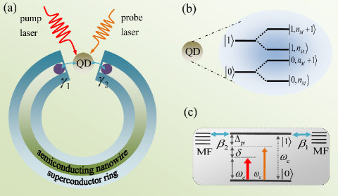
Figure 1 gives the schematic setup that will be studied in this paper, in which a QD coupled to a pair of MFs appearing in the hybrid S/S ring device, and the Hamiltonian is given by LiuDE ; Flensberg1 ; Leijnse ; Pientka ; Sau1 ; Chen03 ; Boyd

$$H = \hbar\omega_{e}S^{z}+i\epsilon_{M}\gamma_{1}\gamma_{2}/2+i\hbar\beta_{1}(S^{-}-S^{{\dagger}})\gamma_{1}$$ (1)

$$+i\hbar\beta_{2}(S^{-}-S^{{\dagger}})\gamma_{2}-\mu E_{c}(S^{{\dagger}}e^{-i\omega_{c}t}+S^{-}e^{i\omega_{c}t})$$

$$-\mu E_{s}(S^{{\dagger}}e^{-i\omega_{s}t}+S^{-}e^{i\omega_{s}t}),$$

where the first term indicates the Hamiltonian of the QD with the exciton frequency $\omega_{e}$. To distinguish from previous theoretical schemes for detecting MFs, where QD is consider as a single resonant level with spin-singlet state LiuDE ; Flensberg1 ; Leijnse ; Pientka ; Sau1 , here we consider the QD is a TLS including the ground state $\left|0\right\rangle$ and the single exciton state $\left|1\right\rangle$ ZrennerA ; StuflerS at low temperature. We introduce the pseudospin operators $S^{z}$ and $S^{\pm}$ with the commutation relations $\left[S^{z},S^{\pm}\right]=\pm S^{\pm}$ and $\left[S^{+},S^{-}\right]=2S^{z}$ to describe the TLS QD.

The second term gives the interaction of a pair of MFs emerging in the hybrid S/S ring device. We use Majorana operators $\gamma_{1}$ and $\gamma_{2}$ to describe MFs satisfying the relation $\gamma^{\dagger}=\gamma$ and $\gamma^{2}=1$ as they are their own antiparticle. Here, $\epsilon_{M}=\hbar\omega_{M}\sim e^{-l/\xi}$ is the coupling energy with $l$ being the semiconductor nanowire length and $\xi$ the superconducting coherent length with Majorana frequency $\omega_{M}$. Obviously, when the semiconductor nanowire length $l$ is large enough, the coupling energy $\epsilon_{M}$ approach zero. Therefore, it is necessary to discuss the two conditions, i.e., the coupled Majorana edge states $\epsilon_{M}\neq 0$ and the uncoupled Majorana edge states $\epsilon_{M}=0$.

The third and the fourth terms describe a pair MFs $\gamma_{1}$ and $\gamma_{2}$ coupled to the QD with the coupling strengths $\beta_{1}$ and $\beta_{2}$, and the coupling strengths relate to the distance of the QD and S/S ring device. For simplicity, we introduce the regular fermion creation (annihilation) operator $f^{{\dagger}}$($f$), and then Majorana operator $\gamma$ can be transformed into the regular fermion operator $f$ with the relation of $\gamma_{1}=f^{{\dagger}}+f$ and $\gamma_{2}$ $=i(f^{{\dagger}}-f)$. Therefore, the third and the fourth terms in Eq. (1) can be rewritten as $i\hbar\beta_{1}(S^{-}f^{{\dagger}}-S^{+}f)-\hbar\beta_{2}(S^{-}f^{{\dagger}}+S^{+}f)$ in the rotating wave approximation RidolfoA , where the non-conservation terms of energy $i\hbar\beta_{1}(S^{-}f-S^{+}f^{+})$ and $\hbar\beta_{2}(S^{-}f+S^{+}f^{+})$ are neglected due to their effect are too small to be considered in our theoretical treatment.

The last two terms in Eq. (1) indicate the interactions between the QD and two laser fields including a strong pump field with frequency $\omega_{c}$ and a weak probe field with frequency $\omega_{s}$ simultaneously irradiating to the QD, where $\mu$ is the electric dipole moment of the exciton, $E_{c}$ and $E_{s}$ are the slowly varying envelope of the pump field and probe field, respectively.

In a frame rotating with the frequency $\omega_{c}$ of the pump field, the Hamiltonian of the system in Eq. (1) can be rewritten as

$$H = \hbar\Delta_{c}S^{z}+\hbar\Delta_{M}(f^{{\dagger}}f-1/2)+i\hbar\beta_{1}(S^{-}f^{{\dagger}}-S^{+}f)$$ (2)

$$-\hbar\beta_{2}(S^{-}f^{{\dagger}}+S^{+}f)-\hbar\Omega_{c}(S^{+}+S^{-})$$

$$-\mu E_{s}(S^{+}e^{-i\delta t}+S^{-}e^{i\delta t}),$$

where $\Delta_{c}=\omega_{e}-\omega_{c}$ is the exciton-pump field detuning, $\Delta_{M}=\omega_{M}-\omega_{c}$ is the Majorana-pump field detuning, and $\delta=\omega_{s}-\omega_{c}$ is the probe-pump detuning. $\Omega_{c}=\mu E_{c}/\hbar$ is the Rabi frequency of the pump field. The Heisenberg-Langevin equations of the operators for the resonators, including the corresponding noise and damping terms, can be written as follows Chen03 ; Walls :

$$\partial_{t}S^{z} = -\Gamma_{1}(S^{z}+1/2)-\beta_{1}(S^{-}f^{{\dagger}}+S^{{\dagger}}f)$$ (3)

$$-i\beta_{2}(S^{-}f^{{\dagger}}+S^{{\dagger}}f)+i\Omega_{c}(S^{{\dagger}}-S^{-})$$

$$+\frac{i\mu E_{s}}{\hbar}(S^{{\dagger}}e^{-i\delta t}-S^{-}e^{i\delta t}),$$

$$\partial_{t}S^{-} = -(i\Delta_{c}+\Gamma_{2})S^{-}+2(\beta_{1}-i\beta_{2})S^{z}f$$ (4)

$$-2i\Omega_{c}S^{z}-\frac{2i\mu E_{s}S^{z}e^{-i\delta t}}{\hbar}+\tau_{in}\text{,}$$

$$\partial_{t}f=-(i\Delta_{M}+\kappa_{M}/2)f+(\beta_{1}+i\beta_{2})S^{-}+\xi\text{,}$$ (5)

where $\Gamma_{1}$ ($\Gamma_{2}$) is the exciton relaxation rate (exciton dephasing rate), and $\kappa_{M}$ is the decay rate of the MFs. $\tau_{in}$ is the $\delta$-correlated Langevin noise operator with zero mean, and $\xi$ is Langevin force arising from the interaction between the Majorana modes and the environment.

Using $S^{z}=S_{0}^{z}+\delta S^{z}$, $S=S_{0}+\delta S$ and $f=f_{0}+\delta f$, Eqs. (3)-(5) can be divided into the steady parts and the fluctuation ones. Substituting the division forms into Eqs. (3)-(5) and setting all the time derivations at the steady parts to be zero, we obtain the steady state solutions of the variables determining the steady-state population inversion ($w_{0}=2S_{0}^{z}$) of the exciton, which obeys the following equation

$$\Gamma_{1}(w_{0}+1)[w_{0}^{2}(\beta_{1}^{2}+\beta_{2}^{2})^{2}-w_{0}(\beta_{1}^{2}+\beta_{2}^{2})(\Gamma_{2}\kappa_{M}-2\Delta_{c}\Delta_{M})$$

$$+(\Delta_{c}^{2}+\Gamma_{2}^{2})(\Delta_{M}^{2}+\kappa_{M}^{2}/4)]+4\Omega_{c}^{2}w_{0}\Gamma_{2}(\Delta_{M}^{2}+\kappa_{M}^{2}/4)=0.$$ (6)

As all the pump fields are assumed to be sufficiently strong, all the operators can be identified with their expectation values under the mean-field approximation $\left\langle Qc\right\rangle=\left\langle Q\right\rangle\left\langle c\right\rangle$ AgarwalGS . After being linearized by neglecting nonlinear terms in the fluctuations, the Langevin equations for the expectation values

$$\left\langle\partial_{t}\delta S^{z}\right\rangle = -\Gamma_{1}\left\langle\delta S^{z}\right\rangle-(\beta_{1}+i\beta_{2})(S_{0}\left\langle\delta f^{{\dagger}}\right\rangle+f_{0}^{\ast}\left\langle\delta S^{-}\right\rangle)$$ (7)

$$-(\beta_{1}-i\beta_{2})(S_{0}^{\ast}\left\langle\delta f\right\rangle+f_{0}\left\langle\delta S^{{\dagger}}\right\rangle)$$

$$+i\Omega_{pu}(\left\langle\delta S^{{\dagger}}\right\rangle-\left\langle\delta S^{-}\right\rangle)$$

$$+\dfrac{i\mu E_{s}}{\hbar}[S_{0}^{\ast}e^{-i\delta t}-S_{0}e^{i\delta t}]\text{,}$$

$$\left\langle\partial_{t}\delta S^{-}\right\rangle = -(i\Delta_{pu}+\Gamma_{2})\left\langle\delta S^{-}\right\rangle+w_{0}(\beta_{1}-i\beta_{2})\left\langle\delta f\right\rangle$$ (8)

$$+2[f_{0}(\beta_{1}-i\beta_{2})-i\Omega_{c}]\left\langle\delta S^{z}\right\rangle$$

$$-\frac{i\mu w_{0}E_{s}}{\hbar}e^{-i\delta t}\text{,}$$

$$\left\langle\partial_{t}\delta f\right\rangle=-(i\Delta_{M}+\kappa_{M}/2)\left\langle\delta f\right\rangle+(\beta_{1}+i\beta_{2})\left\langle\delta S^{-}\right\rangle\text{,}$$ (9)

which is a set of nonlinear equations and the steady-state response in the frequency domain is composed of many frequency components. To solve these equations, we make the ansatz Boyd as $\left\langle\delta O\right\rangle=O_{+}e^{-i\delta t}+O_{-}e^{i\delta t}$ ($O=S^{z},S^{-},f$), and substitute them into Eqs. (7)-(9) with ignoring the second-order terms and working to the lowest order in $E_{s}$ but to all orders in $E_{c}$, we obtain the linear optical susceptibility as $\chi_{eff}^{(1)}(\omega_{s})=\mu S_{+}(\omega_{s})/E_{s}=(\mu^{2}/\hbar\Gamma_{2})\chi^{(1)}(\omega_{s})$, and $\chi^{(1)}(\omega_{s})$ is given by

$$\chi^{(1)}(\omega_{s})=\frac{[{\epsilon}_{7}\Pi_{1}(\Lambda_{4}+\epsilon_{3}\Pi_{2})-iw_{0}\Lambda_{4}]\Gamma_{2}}{{\Lambda_{1}\Lambda_{4}+}\Pi_{1}\Pi_{2}\epsilon_{3}\epsilon_{4}},$$ (10)

where $\Pi_{1}=2[(\beta_{1}-i\beta_{2})f_{0}-i\Omega_{c}]$, $\Pi_{2}=2[(\beta_{1}+i\beta_{2})f_{0}+i\Omega_{c}]$, ${\epsilon}_{1}=(\beta_{1}+i\beta_{2})/[i(\Delta_{M}-\delta)+\kappa_{M}/2]$, ${\epsilon}_{2}=(\beta_{1}+i\beta_{2})/[i(\Delta_{M}+\delta)+\kappa_{M}/2]$, ${\epsilon}_{3}=[i\Omega_{c}-(\beta_{1}-i\beta_{2})f_{0}-(\beta_{1}+i\beta_{2})S_{0}{\epsilon}_{2}^{\ast}]/(\Gamma_{1}-i\delta)$, ${\epsilon}_{4}=[i\Omega_{c}+(\beta_{1}+i\beta_{2})f_{0}^{\ast}+(\beta_{1}-i\beta_{2})S_{0}^{\ast}{\epsilon}_{1}]/(\Gamma_{1}-i\delta)$, ${\epsilon}_{5}=[i\Omega_{c}-(\beta_{1}-i\beta_{2})f_{0}-(\beta_{1}+i\beta_{2})S_{0}{\epsilon}_{1}^{\ast}]/(\Gamma_{1}+i\delta)$, ${\epsilon}_{6}=[i\Omega_{c}+(\beta_{1}+i\beta_{2})f_{0}^{\ast}+(\beta_{1}-i\beta_{2})S_{0}^{\ast}{\epsilon}_{2}]/(\Gamma_{1}+i\delta)$, ${\epsilon}_{7}=iS_{0}^{\ast}/(\Gamma_{1}-i\delta)$, ${\epsilon}_{8}=iS_{0}/(\Gamma_{1}+i\delta)$, ${\Lambda_{1}=i(\Delta_{c}-\delta)}+\Gamma_{2}-w_{0}(\beta_{1}-i\beta_{2}){\epsilon}_{1}+\Pi_{1}\epsilon_{4}$, ${\Lambda_{2}=-i(\Delta_{c}-\delta)}+\Gamma_{2}-w_{0}(\beta_{1}+i\beta_{2}){\epsilon}_{1}^{\ast}-\Pi_{2}\epsilon_{5}$, ${\Lambda_{3}=i(\Delta_{c}+\delta)}+\Gamma_{2}-w_{0}(\beta_{1}-i\beta_{2}){\epsilon}_{2}+\Pi_{1}\epsilon_{6}$, ${\Lambda_{4}=-i(\Delta_{c}+\delta)}+\Gamma_{2}-w_{0}(\beta_{1}+i\beta_{2}){\epsilon}_{1}+\Pi_{2}\epsilon_{3}$. The imaginary and real parts of $\chi^{(1)}(\omega_{s})$ indicate absorption and dispersion, respectively.

Based on the hybrid QD-S/S ring device, we can determine the light group velocity as Harris ; Bennink $v_{g}=c/[n+\omega_{s}(dn/d\omega_{s})]$ where $n\approx 1+2\pi\chi_{eff}^{(1)}$. Therefore

$$c/v_{g} = 1+2\pi Re\chi_{eff}^{(1)}(\omega_{s})_{\omega_{s}=\omega_{e}}$$ (11)

$$+2\pi\omega_{s}Re(d\chi_{eff}^{(1)}/d\omega_{s})_{\omega_{s}=\omega_{e}}\text{.}$$

Obviously, when $Re\chi_{eff}^{(1)}(\omega_{s})_{\omega_{s}=\omega}=0$, the dispersion is steeply positive or negative, and the group velocity is significantly reduced or increased. Thus we define the group velocity index $n_{g}$ as

$$n_{g} = \dfrac{c}{v_{g}}-1=\dfrac{c-v_{g}}{v_{g}}$$ (12)

$$= \frac{2\pi\omega_{e}\rho\mu^{2}}{\hbar\Gamma_{2}}Re(\frac{d\chi_{eff}^{(1)}}{d\omega_{s}})_{\omega_{s}=\omega_{e}}$$

$$= \Gamma_{2}\Sigma Re(\frac{d\chi_{eff}^{(1)}}{d\omega_{s}})_{\omega_{s}=\omega_{e}}\text{,}$$

where $\Pi=2\pi\omega_{e}\rho\mu^{2}/\hbar\Gamma_{2}$. One can observe the slow light when $n_{g}>0$, and the superluminal light when $n_{g}<0$ Boyd01 .

The parameter values used in the paper MourikV ; DasA ; DengMT ; Nadj-PergeS2 ; Chen03 ; Wilson-RaeI : the QD-MFs coupling strength $\beta_{1}=\beta_{2}=0.05$ GHz, the decay rate of the MFs $\kappa_{M}=0.1$ MHz, $\Gamma_{1}=0.3$ GHz, $\Gamma_{2}=0.15$ GHz, and $\Omega_{pu}^{2}=0.005($GHz$)^{2}$.

III MMIT, Fano resonance, and tunable switch of fast-to-slow light

III.1 Case A: the exciton-pump field detuning $\Delta_{c}=0$ and $\Delta_{c}=0.5$ GHz under uncoupled Majorana modes $\Delta_{M}=0$ ($\epsilon_{M}=0$), respectively.

In Fig. 1, we first consider the condition of uncoupled Majorana modes, i.e., $\Delta_{M}=0$ or $\epsilon_{M}=0$ under the exciton-pump field detuning $\Delta_{c}=0$. Then the Hamiltonian of the coupled QD-MFs system reduce to $H_{MFs-QD}=i\hbar\beta_{1}(S^{-}f^{{\dagger}}-S^{+}f)-\hbar\beta_{2}(S^{-}f^{{\dagger}}+S^{+}f)$ which is similar to J-C Hamiltonian of standard model, and no the term of $\hbar\Delta_{M}(f^{{\dagger}}f-1/2)$ in Eq.(1). Therefore, the probe absorption spectra will present symmetric splitting. Figure 2(a) gives the imaginary part of the dimensionless susceptibility Im$\chi^{(1)}$ which indicates the probe absorption spectra of the probe field as a function of the probe detuning $\Delta_{s}=\omega_{s}-\omega_{e}$ under four different QD-MFs coupling strengths $\beta_{2}$ under $\beta_{1}=0.05$ GHz. The black curve in Fig.2(a) shows the result of only considering the QD-MFs coupling $\beta_{1}$, and the probe absorption spectrum shows a symmetric splitting. With increasing the QD-MFs coupling strengths $\beta_{2}$, the distance of the splitting is enhanced significantly, and the bigger QD-MFs coupling $\beta_{2}$ induced larger peak width of splitting. Figure 2(b) shows the dispersion of the probe light in the case $\Delta_{c}=0$ under uncoupled Majorana modes for several different QD-MFs coupling strengths $\beta_{2}$ with $\beta_{1}=0.05$ GHz. When increasing the coupling strength $\beta_{2}$ from $\beta_{2}=0$ to $\beta_{2}=3\beta_{1}$, the dispersion of the probe light varies from negative to positive around $\Delta_{s}=0$, which results in positive group delay or slow light propagation through the system. Therefore, the change of dispersion from negative to positive slope with manipulating the coupling strength $\beta_{2}$ corresponds to the control of fast-to-slow light propagation. In Fig.2(c), we further present three different QD-MFs coupling strength including ($\beta_{1}=0.05$ GHz, $\beta_{2}=0.05$ GHz), ($\beta_{1}=0.07$ GHz, $\beta_{2}=0.03$ GHz), and ($\beta_{1}=0.09$ GHz, $\beta_{2}=0.01$ GHz), which also manifests a symmetric splitting in the probe absorption spectrum, and Fig.2(d) gives the dispersion of the probe light in this condition. The physical origin of such results are due to the coherent interaction between the QD and MFs, and here we introduce the dressed state theory between the QD and MFs to interpret this physical phenomena. As the QD is consider as a TLS with the ground state $\left|0\right\rangle$ and exciton state $\left|e\right\rangle$, when QD couple to MFs, the two-level QD will modify by the number states of the MFs $n_{M}$ ($n_{M}$ is the number states of the MFs) generating the Majorana dressed states $\left|0,n_{M}\right\rangle$, $\left|0,n_{M}+1\right\rangle$, $\left|1,n_{M}\right\rangle$, $\left|1,n_{M}+1\right\rangle$. The left sharp peak of splitting in the probe absorption spectra indicate the transition from $\left|0\right\rangle$ to $\left|1,n_{M}\right\rangle$, and the right sharp peak is due to the transition of $\left|0\right\rangle$ to $\left|1,n_{M}+1\right\rangle$. In addition, the probe absorption spectra show the analogous phenomenon of electromagnetically induced transparency (EIT) (the symmetric splitting) FleischhauerM in $\Lambda$-type atoms systems. Due to it is majorana modes induced such phenomenon, and then we term the phenomenon as Majorana modes induced transparency (MMIT). Obviously, the absorption dip approaches zero around $\Delta_{s}=0$ under uncoupled Majorana modes $\epsilon_{M}=0$, which means the input probe field is transmitted to the coupled system without experiencing any absorption.

Figure 2: (a) The probe absorption spectra of the probe field as a function of the probe detuning $\Delta_{s}=\omega_{s}-\omega_{e}$ under four different QD-MFs coupling strengths $\beta_{2}$ under $\beta_{1}=0.05$ GHz and (b) gives their dispersion of the probe light in this condition. (c) plots three different QD-MFs coupling strengths $\beta_{1}$ and $\beta_{2}$ and (d) is the related dispersion. The detuning conditions are $\Delta_{c}=0$ and $\Delta_{M}=0$.

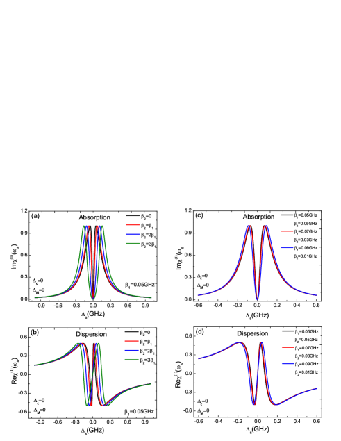
When switching the exciton-pump field detuning $\Delta_{c}$ from $\Delta_{c}=0$ and $\Delta_{c}=0.5$ GHz, the probe absorption spectra experience the symmetric splitting (i.e., EIT) to unsymmetric splitting (i.e., Fano resonance) under the condition of uncoupled majorana modes $\epsilon_{M}=0$ as shown in Fig. 3. Figure 3(a) displays the probe absorption spectra presenting Fano resonance under several different QD-MFs coupling strengths $\beta_{2}$ with $\beta_{1}=0.05$ GHz, and Fig. 3(b) is its detail around $\Delta_{s}=0$. It is obvious that the unsymmetric splitting is increased with bigger QD-MFs coupling strengths $\beta_{2}$. Figure 3(c) plots the dispersion of the probe light for four different QD-MFs coupling strengths $\beta_{2}$ and Fig. 3(d) is its detail. We see that there is a steep positive slope around $\Delta_{s}=0$, which signifies the potential of ultraslow light achievement. Compared with Fig.2(a) and Fig.2(c), the absorption dip in Fig. 3(a) also approaches zero around $\Delta_{s}=0$, which is also analogous EIT without experiencing any absorption. However, the physical regimes are different from in Fig. 2. The results are ascribed to the destructive quantum interference effect between Majorana modes and the beat frequency $\delta$ of the two input laser fields irradiating on the QD. Once the beat frequency $\delta$ approximates to the resonance frequency $\omega_{M}$ of Majorana modes, Majorana modes begin oscillating coherently resulting in Stokes-like ($\Delta_{S}=\omega_{c}-\omega_{M}$) and anti-Stokes-like ($\Delta_{A-S}=\omega_{c}+\omega_{M}$) scattering of light from the QD. When the condition is highly off-resonant ($\Delta_{c}=0.5$ GHz), the Stokes-like scattering is strongly suppressed, and only leaving the anti-Stokes-like field interferes with the near-resonant probe field modifying the probe absorption spectra. As a result, the probe absorption spectra present zero absorption, i.e., MMIT.

Figure 3: (a) The probe absorption spectra under several different QD-MFs coupling strengths $\beta_{2}$ with $\beta_{1}=0.05$ GHz, and (b) is its detail aroud $\Delta_{s}=0$. (c) The dispersion of the probe light for four different QD-MFs coupling strengths $\beta_{2}$, and (d) is its detail. The detuning conditions are $\Delta_{c}=0.5$ GHz and $\Delta_{M}=0$.

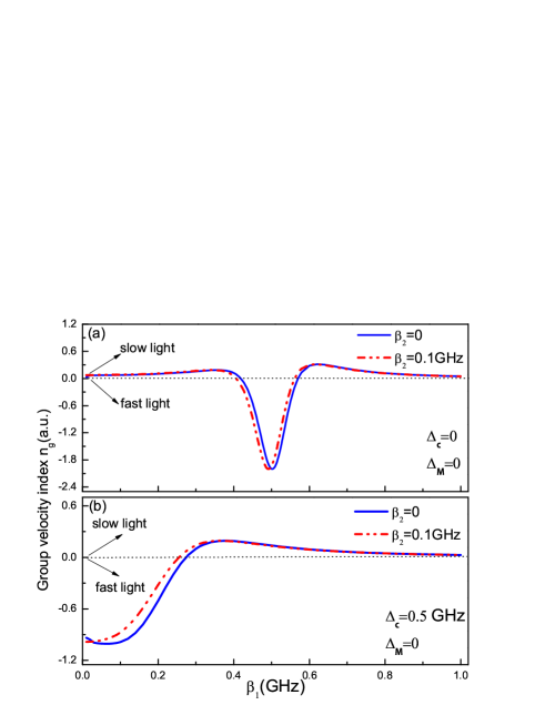
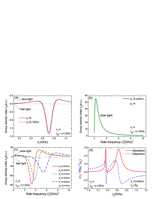
No matter what regimes induce the zero absorption in the probe absorption spectra, once MMIT appear in the hybrid coupled system, the remarkable phenomena of slow light or fast light can appear in the hybrid system. The dispersion of the probe light in Fig.2(b) and Fig.3(d) show the dispersion experiencing negative to positive slope with controlling the coupling strength $\beta_{2}$ corresponds to the control of fast-to-slow light propagation. In Fig.4(a), we consider the condition of $\Delta_{c}=0$ and $\Delta_{M}=0$. Figure 4(a) plots the group velocity index $n_{g}$ of probe laser (in the unit of $\Pi$) as a function of one of QD-MFs coupling strengths $\beta_{1}$ under two cases of $\beta_{2}=0$ and $\beta_{2}=0.1$ GHz, respectively. It is obvious that group velocity index $n_{g}$ experiences the change of positive-negative-positive, which corresponds to the slow-fast-slow light in the both two conditions, respectively. In Fig.4(b), we consider the condition of $\Delta_{c}=0.5$ GHz and $\Delta_{M}=0$. We further show the group velocity index $n_{g}$ as a function of $\beta_{1}$ under the cases of $\beta_{2}=0$ and $\beta_{2}=0.1$ GHz, respectively, which presents $n_{g}$ experiencing the switch from fast to slow light.

Figure 4: (a) The group velocity index $n_{g}$ of probe laser as a function of $\beta_{1}$ under two cases of $\beta_{2}=0$ and $\beta_{2}=0.1$ GHz under $\Delta_{c}=0$ and $\Delta_{M}=0$, respectively. (b) The group velocity index $n_{g}$ as a function of $\beta_{1}$ under the cases of $\beta_{2}=0$ and $\beta_{2}=0.1$ GHz under $\Delta_{c}=0.5$ GHz and $\Delta_{M}=0$, respectively.

III.2 Case B: the exciton-pump field detuning $\Delta_{c}=0$ under coupled Majorana modes $\epsilon_{M}\neq 0$

When the semiconductor nanowire length $l$ is large enough, the coupling energy $\epsilon_{M}$ approach zero. For the realistic device, length $l$ is limited, and then $\epsilon_{M}\neq 0$. Therefore, it is necessary to discuss the condition, of the coupled Majorana edge states $\epsilon_{M}\neq 0$. In Fig.5, we discuss the Fano resonance on the condition of coupled Majorana modes ($\epsilon_{M}\neq 0$). Figure 5(a) plots the probe absorption spectra under $\Delta_{c}=0$ for several different QD-MFs coupling strengths $\beta_{2}$ with $\beta_{1}=0.05$ GHz, and Fig. 5(b) is its detail. With increasing the coupling strengths $\beta_{2}$, the splitting of the two peaks is broadened. In this case, the transparency windows locate at $\Delta_{s}=-0.5$ GHz, which is different from in Fig.3(a) locating at $\Delta_{s}=0$. Figure 5(c) plots the dispersion of the probe light with four coupling strengths $\beta_{2}$ and Fig. 5(d) is its detail, which has the same process of evolution as in Fig.3(c).

Figure 5: (a) The probe absorption spectra under four QD-MFs coupling strengths $\beta_{2}$ with $\beta_{1}=0.05$ GHz, and (b) is its detail aroud $\Delta_{s}=0$. (c) The dispersion of the probe light for four different QD-MFs coupling strengths $\beta_{2}$, and (d) is its detail. The detuning conditions are $\Delta_{c}=0$ and $\Delta_{M}=-0.5$ GHz.

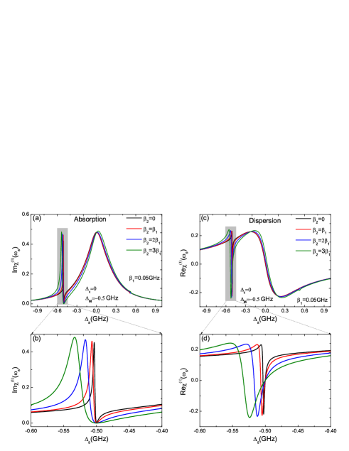
Figure 6 plots the group velocity index $n_{g}$ of probe laser under different parameter regimes. In Fig.6(a), we investigate the group velocity index $n_{g}$ as a function of $\beta_{1}$ under the condition of $\beta_{2}=0$ and $\beta_{2}=0.1$ GHz, respectively, which presents the same evolution as in Fig.4(a) indicating the slow-fast-slow light in the hybrid system. We further discuss several different QD-MFs coupling strengths, such as ($\beta_{2}=0.05$ GHz, $\beta_{2}=0$), ($\beta_{2}=0.05$ GHz, $\beta_{2}=0.05$ GHz), ($\beta_{2}=0.07$ GHz, $\beta_{2}=0.03$ GHz), and ($\beta_{2}=0.09$ GHz, $\beta_{2}=0.01$ GHz), which influences the group velocity index $n_{g}$. Figure 6(b) plots the group velocity index $n_{g}$ of probe laser versus the Rabi frequency $\Omega_{pu}^{2}$ of the pump field in the case of $\beta_{1}=0.05$ GHz and $\beta_{2}=0$ under the condition of $\Delta_{c}=0$ and $\epsilon_{M}\neq 0$. One can see from Fig. 6(b) that the group velocity index $n_{g}$ is positive when the Rabi frequency varies, which represent the slow light effect. Figure 6(c) presents the group velocity index $n_{g}$ vs. Rabi frequency $\Omega_{pu}^{2}$ under other three conditions, i.e., ($\beta_{2}=0.05$ GHz, $\beta_{2}=0.05$ GHz), ($\beta_{2}=0.07$ GHz, $\beta_{2}=0.03$ GHz), and ($\beta_{2}=0.09$ GHz, $\beta_{2}=0.01$ GHz). When the QD is close to one MF (such as $\gamma_{1}$, and then $\beta_{1}>\beta_{2}$), the experience of the group velocity index $n_{g}$ is different from the case of $\beta_{1}=\beta_{2}$, which can reach the switch of slow to fast light. The QD-MFs coupling strength can be controlled via adjusting the distance of the QD and the hybrid S/SR device. Therefore, with controlling the QD-MFs coupling strengths, the fast-to-slow light or vice versa can be achieved straightforward in the hybrid system. In Fig.6(d), we further give much more bigger coupling strengths $\beta_{2}$ ($\beta_{2}=5\beta_{1}$) that influence the absorption and dispersion of the QD. Obviously, the absorption and dispersion are enhanced with bigger $\beta_{2}$ that induce distinct Fano resonance and optical propagation, respectively.

Figure 6: (a) The group velocity index $n_{g}$ as a function of $\beta_{1}$ under the condition of $\beta_{2}=0$ and $\beta_{2}=0.1$ GHz, respectively. (b) The group velocity index $n_{g}$ versus the Rabi frequency $\Omega_{pu}^{2}$ in the case of $\beta_{1}=0.05$ GHz and $\beta_{2}=0$. (c) The group velocity index $n_{g}$ vs. Rabi frequency $\Omega_{pu}^{2}$ under other three conditions. (d) The absorption and dispersion of the QD in much more bigger coupling strengths $\beta_{2}$ ($\beta_{2}=5\beta_{1}$). The detuning conditions are $\Delta_{c}=0$ and $\Delta_{M}=-0.5$ GHz.

III.3 Case C: the exciton-pump field detuning off-resonant $\Delta_{c}\neq 0$ under coupled Majorana modes $\epsilon_{M}\neq 0$

In this case, we first adjust the detuning $\Delta_{c}$ from $\Delta_{c}=0$ to $\Delta_{c}=0.5$ GHz under coupled Majorana modes $\epsilon_{M}\neq 0$. Figure 7(a) gives the probe absorption spectra with several different QD-MFs coupling strengths $\beta_{2}$ for $\beta_{1}=0.05$ GHz under the condition of $\Delta_{M}=-0.5$ GHz and $\Delta_{c}=0.5$ GHz, which shows more remarkable Fano resonance and the intensity is also enhanced simultaneously. Figure 7(b) is the detail parts of the left peaks in Fig.7(a). Compared with Fig.3(a) and Fig.5(a), we find the splitting distance in Fig.7(a) is the sum of the splitting distance in Fig.3(a) and Fig.5(a), i.e., the splitting distance is $\Delta_{c}-\Delta_{M}$. Figure 7(c) plots the dispersion of the probe light with four coupling strengths $\beta_{2}$ and Fig. 7(d) is its detail. Therefore, the remarkable fast to slow light (or vice versa) can also be achieved in this condition.  Moreover, when we make a comparison between the conditions in Case C and Case A (or Case B), we find the full width at half maximum (FWHM) is narrower in Case C than in Case A (or Case B), as well as the stronger intensity. So, the sideband peak induced by coupled Majorana modes coincides with sharp peaks induced by pump off-resonant $\Delta_{c}\neq 0$, which makes the coherent interaction of QD-MF more strong.

Figure 7: (a) The probe absorption spectra for several different QD-MFs coupling strengths $\beta_{2}$ at $\beta_{1}=0.05$ GHz, and (b) is the detail parts of the left peaks. (c) The dispersion of the probe light with four coupling strengths $\beta_{2}$ and (d) is its detail. The detuning conditions are $\Delta_{M}=-0.5$ GHz and $\Delta_{c}=0.5$ GHz,

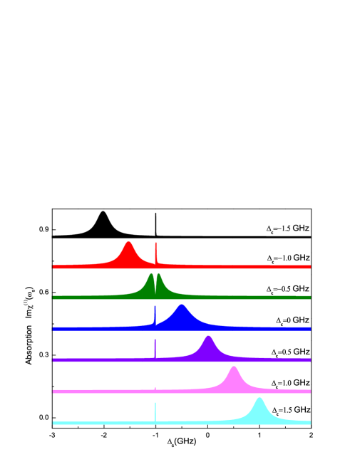
We then change the exciton-pump field detuning $\Delta_{c}$ from $\Delta_{c}=-1.5$ GHz to $\Delta_{c}=1.5$ GHz under $\Delta_{M}=-0.5$ GHz, the scenario of absorption becomes completely different. Figure 8 shows the probe absorption spectra as a function of $\Delta_{s}$ with fixed pump intensity $\Omega_{pu}^{2}=0.005($GHz$)^{2}$, which experiences the switch from Fano resonance to EIT to Fano resonance with the change of the detuning $\Delta_{c}$. It is obvious that these Majorana-induced resonances have a Fano-like shape that varies with the detuning $\Delta_{c}$. When the drive-resonance detuning $\Delta_{c}=\Delta_{M}$, the Fano-like resonance changes into a symmetric Lorentzian-shaped absorption peak (i.e., MMIT). In addition, we find that the transparency windows (the absorption dip approaches zero) still locate at $\Delta_{s}=-1.0$ GHz. However, the Lorentz peaks vary with the change of the detuning $\Delta_{c}$ and locate at $\Delta_{c}+\Delta_{M}$. This behavior may be ascribed to the off-resonant coupling between the QD and MFs. In addition, the probe absorption splits into two resonances, known as the Autler-Townes (AT) splitting, is also observed in strongly driven quantum dot system XuX , where the probe absorption spectra display symmetrical splitting when the pump is on resonance and show unsymmetric splitting at off-resonance. When we consider a pair of MFs coupled to the QD, the evolution of the absorption changes significantly and the probe absorption spectra are very different from a single QD system. This further demonstrate the role of MFs in the hybrid system, and MFs provide a quantum channel to affect the probe absorption. Obviously, the absorption spectra can be modified effectively via the off-resonant coupling between the QD and MFs.

Figure 8: The probe absorption spectra as a function of $\Delta_{s}$ with fixed pump intensity $\Omega_{pu}^{2}=0.005($GHz$)^{2}$ for seven different detuning $\Delta_{c}$ under $\Delta_{M}=-0.5$ GHz.

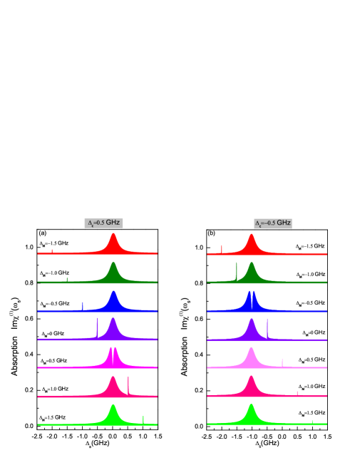
On the other hand, we discuss the variation of the probe absorption spectra under two conditions of $\Delta_{c}=0.5$ GHz and $\Delta_{c}=-0.5$ GHz with change the Majorana-pump field detuning $\Delta_{M}$ from $\Delta_{M}=-1.5$ GHz to $\Delta_{M}=1.5$ GHz, respectively. Figure 9(a) plots a series of probe absorption spectra under $\Delta_{c}=0.5$ GHz with several different $\Delta_{M}$. In this condition, Fano resonance vary significantly and Lorentz-like peaks locate at $\Delta_{s}=0$, except $\Delta_{M}=0.5$ GHz presenting EIT. The location of the transparency windows (i.e., the absorption dip approaches zero) vary with the change of $\Delta_{M}$, and we find that the distance of the splitting is $\Delta_{M}-\Delta_{c}$. Figure 9(b) gives a series of probe absorption spectra under $\Delta_{c}=-0.5$ GHz with seven different $\Delta_{M}$. In this situation, the evolution of Fano resonances are also remarkable and Lorentz-like peaks locate at $\Delta_{s}=-1.0$ GHz, but the phenomenon of EIT locating at $\Delta_{M}=-1.0$ GHz, and the distance of the splitting of two peaks is also $\Delta_{M}-\Delta_{c}$. Compared with Fig. 9(a) and Fig. 9(b), we find probe absorption spectra at $\Delta_{M}=\Phi$ and $\Delta_{M}=-\Phi$ ($\Phi$ indicates numerical value) presenting mirror symmetry, such as $\Delta_{M}=1.5$ GHz and $\Delta_{M}=-1.5$ GHz, and so on.

Figure 9: A series of probe absorption spectra under $\Delta_{c}=0.5$ GHz with several different $\Delta_{M}$. (b) A series of probe absorption spectra under $\Delta_{c}=-0.5$ GHz with seven different $\Delta_{M}$.

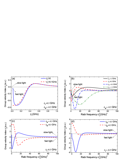
In Fig. 10, we plot the group velocity index $n_{g}$ of probe laser under different detuning regimes. In Fig.10(a), we investigate the group velocity index $n_{g}$ as a function of $\beta_{1}$ for $\beta_{2}=0$ and $\beta_{2}=0.1$ GHz under $\Delta_{c}=0.5$ GHz and $\Delta_{M}=-0.5$ GHz, respectively, which presents the conversion from fast to slow light. When $\beta_{1}<0.1$ GHz, the experience of the group velocity index $n_{g}$ is a little difference, while when $\beta_{1}>0.1$ GHz, the two curves are approximate coincide. Figure 10(b) shows the group velocity index $n_{g}$ of probe laser versus the Rabi frequency $\Omega_{pu}^{2}$ of the pump field corresponding to Fig.8, and we only plot four curves at four different detuning $\Delta_{c}$ under $\Delta_{M}=-0.5$ GHz. Obviously, the group velocity index $n_{g}$ undergo advance to delay corresponding to fast to slow light. Figure 10(c) plots the group velocity index $n_{g}$ versus the Rabi frequency $\Omega_{pu}^{2}$ corresponding to Fig.9(a), and we give two curves at $\Delta_{M}=-0.5$ GHz (the blue one) and $\Delta_{M}=0.5$ GHz (the red one) under $\Delta_{c}=0.5$ GHz, which indicates the conversion from fast to slow light and slow to fast light, respectively. Figure 10(d) plots the group velocity index $n_{g}$ versus the Rabi frequency $\Omega_{pu}^{2}$ corresponding to Fig.9(b), and we give two curves at $\Delta_{M}=-0.5$ GHz (the blue one) and $\Delta_{M}=0.5$ GHz (the red one) under $\Delta_{c}=-0.5$ GHz. Compared with Fig. 10(c), although it can also obtain the conversion from fast to slow light and vice versa, the process of evolution is a little different from in Fig.10(c). Thus, with controlling different detuning regimes, the fast-to-slow light or vice versa can be achieved straightforward in the hybrid system.

Figure 10: (a) The group velocity index $n_{g}$ as a function of $\beta_{1}$ for $\beta_{2}=0$ and $\beta_{2}=0.1$ GHz under $\Delta_{c}=0.5$ GHz and $\Delta_{M}=-0.5$ GHz, respectively, (b) The group velocity index $n_{g}$ of probe laser versus the Rabi frequency $\Omega_{pu}^{2}$ of the pump field for four different detuning $\Delta_{c}$ under $\Delta_{M}=-0.5$ GHz. (c) The group velocity index $n_{g}$ versus the Rabi frequency $\Omega_{pu}^{2}$ under $\Delta_{M}=-0.5$ GHz and $\Delta_{M}=0.5$ GHz with $\Delta_{c}=0.5$ GHz. (d) The group velocity index $n_{g}$ versus the Rabi frequency $\Omega_{pu}^{2}$ at $\Delta_{M}=-0.5$ GHz and $\Delta_{M}=0.5$ GHz for under $\Delta_{c}=-0.5$ GHz.

IV Conclusion

We have investigated the Fano resonance and coherent optical propagation properties in the hybrid QD-S/S ring device, which includes a QD driven by two-tone fields coupled to a couple of MFs emerging in the ends of the nanowire of the hybrid S/S ring device. We found Majorana modes induced transparency, the Fano resonances and their related propagation properties such as fast and slow light effects can achieved under different parameter regimes, such as the exciton-pump field detuning $\Delta_{c}$, the Majorana-pump field detuning $\Delta_{M}$, and the QD-MFs coupling strengths $\beta_{1}$ and $\beta_{2}$. With controlling the detuning of $\Delta_{c}$ and $\Delta_{M}$, a series of asymmetric Fano line shapes can appear and the positions of the Fano line shapes are closely related to the two detuning. In addition, the fast-to-slow light or vice versa can be achieved in the hybrid system by controlling different detuning regimes. The scheme proposed here may provide potential applications in all-optically controlled quantum computing based on MFs in solid-state devices.

References

- (1) M. Fleischhauer, A. Imamoglu, J. P. Marangos, Rev. Mod. Phys. 77, 633 (2005).
- (2) L. V. Hau, S. E. Harris, Z. Dutton, and C. H. Behroozi, Nature 397, 594 (1999).
- (3) D. Budker, D. F. Kimball, S. M. Rochester, and V. V. Yashchuk, Phys. Rev. Lett. 83, 1767 (1999).
- (4) C. Liu, Z. Dutton, C. H. Behroozi, and L. V. Hau, Nature, 409, 490 (2001).
- (5) S. E. Harris, J. E. Field, and A. Imamoglu, Phys. Rev. Lett. 64, 1107 (1990).
- (6) J. Q. Shen and S. He, Phys. Rev. A 74, 063831 (2006).
- (7) J. Q. Shen, Phys. Rev. A 90, 023814 (2014).
- (8) U. Fano, Phys. Rev. 124, 1866 (1961).
- (9) A. E. Miroshnichenko, S. Flach, and Y. S. Kivshar, Rev. Mod. Phys. 82, 2257 (2010).
- (10) J. Guo, L. Jiang, Y. Jia, X. Dai, Y. Xiang, and D. Fan, Opt. Express 25, 5972 (2017).
- (11) S. Nojima, M. Usuki, M. Yawata, and M. Nakahata, Phys. Rev. A 85, 063818 (2012).
- (12) A. Artar, Y. Ahmet Ali, and H. Altug, Nano Lett. 11, 3694(2011).
- (13) K.-L. Lee, S.-H. Wu, C.-W. Lee, and P.-K. Wei, Opt. Express 19, 24530 (2011).
- (14) Z.-K. Zhou, X.-N. Peng, Z.-J. Yang, Z.-S. Zhang, M. Li, X.-R. Su, Q. Zhang, X. Shan, Q.-Q.Wang, and Z. Zhang, Nano. Lett. 11, 49(2011).
- (15) C. Wu, A. B. Khanikaev, and G. Shvets, Phys. Rev. Lett. 106, 107403 (2011).
- (16) Alicea, J. Rep. Prog. Phys. 75, 076501 (2012).
- (17) V. Mourik, K. Zuo, S. M. Frolov, S. R. Plissard, E. P. A. M. Bakkers, and L. P. Kouwenhoven. Science, 336, 1003 (2012).
- (18) A. Das, Y. Ronen, Y. Most, Y. Oreg, M. Heiblum and H. Shtrikman. Nat. Phys. 8, 887 (2012).
- (19) M. T. Deng, C. L. Yu, G. Y. Huang, M. Larsson, P. Caroff, and H. Q. Xu, Nano Lett. 12, 6414 (2012).
- (20) S. Nadj-Perge, I. K. Drozdov, J. Li, H. Chen, S. Jeon, J. Seo, A. H. MacDonald, B. A. Bernevig, A. Yazdani, Science, 346, 602 (2014).
- (21) J. Chen, P. Yu, J. Stenger, M. Hocevar, D. Car, S. R. Plissard, E. P. A. M. Bakkers, T. D. Stanescu, and S. M. Frolov, Sci. Adv. 2017, 3: e1701476
- (22) J.-X. Yin, Z. Wu, J.-H. Wang, Z.-Y. Ye, J. Gong, X.-Y. Hou, L. Shan, A. Li, X.-J. Liang, X.-X. Wu, J. Li, C.-S. Ting, Z.-Q. Wang, J.-P. Hu, P.-H. Hor, H. Ding, and S. H. Pan, Nat. Phys., 11, 543 (2015).
- (23) S. M. Albrecht, A. P. Higginbotham, M. Madsen, F. Kuemmeth, T. S. Jespersen, J. Nygård, P. Krogstrup, and C. M. Marcus, Nature, 531, 206 (2016).
- (24) H.-H. Sun, K.-W. Zhang, L.-H. Hu, C. Li, G.-Y. Wang, H.-Y. Ma, Z.-A. Xu, C.-L. Gao, D.-D. Guan, Y.-Y. Li, C. Liu, D. Qian, Y. Zhou, L. Fu, S.-C. Li, F.-C. Zhang, and J.-F. Jia, Phys. Rev. Lett., 116, 257003 (2016).
- (25) Q. L. He, L. Pan1, A. L. Stern, E. C. Burks, X. Che, G. Yin, J. Wang, B. Lian, Q. Zhou, E. S. Choi, K. Murata, X. Kou1, Z. Chen, T. Nie, Q. Shao, Y. Fan, S.-C. Zhang, K. Liu, J. Xia, K. L. Wang, Science, 357, 294 (2017).
- (26) S. R. Elliott, M. Franz, Rev. Mod. Phys. 87, 137 (2015).
- (27) L. P. Rokhinson, X. Liu, J. K. Furdyna, Nat. Phys. 8, 795 (2012).
- (28) S. Jeon, Y. Xie, J. Li, Z. Wang, B. A. Bernevig, A. Yazdani, Science, 358, 772 (2017).
- (29) B. Urbaszek, X. Marie, T. Amand, O. Krebs, P. Voisin, P. Maletinsky, A. Högele, and A. Imamoglu, Rev. Mod. Phys, 85, 79 (2013).
- (30) D. E. Liu, H. U. Baranger, Phys. Rev. B 84, 201308(R) (2011).
- (31) K. Flensberg, Phys. Rev. Lett. 106, 090503 (2011).
- (32) M. Leijnse, K. Flensberg, Phys. Rev. B 84, 140501(R) (2011).
- (33) F. Pientka, G. Kells, A. Romito, P. W. Brouwer, and F. von Oppen, Phys. Rev. Lett. 109, 227006 (2012).
- (34) J. D. Sau, S. D. Sarma, Nat. Commu., 3, 964 (2012).
- (35) M. T. Deng, S. Vaitiekėnas, E. B. Hansen, J. Danon, M. Leijnse, K. Flensberg, J. Nygård, P. Krogstrup, C. M. Marcus, Science, 354, 1557 (2016).
- (36) H. J. Chen, K. D, Zhu, Nanoscale Res. Lett. 9, 166 (2014).
- (37) H. J. Chen, X. W. Fang, C. Z. Chen, Y. Li, X. D. Tang, Sci. Rep. 6, 36600 (2016).
- (38) H. J. Chen, H. W. Wu, Sci. Rep, 8, 17677 (2018).
- (39) R. W. Boyd, Nonlinear Optics. (Academic Press, Amsterdam, 2008).
- (40) A. Zrenner, E. Beham, S. Stufler, E. Findeis, M. Bichler, and G. Abstreiter, Nature (London) 418, 612 (2002).
- (41) S. Stufler, P. Ester, A. Zrenner, and M. Bichler Phys. Rev. B 72, 121301 (2005).
- (42) A. Ridolfo, O. D. Stefano, N. Fina, R. Saija, S. Savasta, Phys. Rev. Lett. 105, 263601 (2010).
- (43) D. F. Walls, and G. J. Milburn, Quantum Optics (Springer, 1994) p. 245
- (44) G. S. Agarwal, S. Huang, Phys. Rev. A 81, 041803 (2010).
- (45) S. E. Harris, J. E. Field, A. Kasapi, Phys. Rev. A 46, R29 (1992).
- (46) R. S. Bennink, R. W. Boyd, C. R. Stroud, V. Wong, Phys. Rev. A 63, 033804 (2001).
- (47) R. W. Boyd, D.J. Gauthier, Science 326, 1074 (2009).
- (48) I. Wilson-Rae, P. Zoller, and A. Imamoḡlu, Phys. Rev. Lett. 92, 075507 (2004).
- (49) X. Xu, B. Sun, P. R. Berman, D. G. Steel, A. S. Bracker, D. Gammon, and L. J. Sham, Science 317, 929 (2007).