A GraphBLAS Approach for Subgraph Counting

Abstract.

Subgraph counting aims to count the occurrences of a subgraph template T in a given network G. The basic problem of computing structural properties such as counting triangles and other subgraphs has found applications in diverse domains. Recent biological, social, cybersecurity and sensor network applications have motivated solving such problems on massive networks with billions of vertices. The larger subgraph problem is known to be memory bounded and computationally challenging to scale; the complexity grows both as a function of T and G. In this paper, we study the non-induced tree subgraph counting problem, propose a novel layered software-hardware co-design approach, and implement a shared-memory multi-threaded algorithm: 1) reducing the complexity of the parallel color-coding algorithm by identifying and pruning redundant graph traversal; 2) achieving a fully-vectorized implementation upon linear algebra kernels inspired by GraphBLAS, which significantly improves cache usage and maximizes memory bandwidth utilization. Experiments show that our implementation improves the overall performance over the state-of-the-art work by orders of magnitude and up to 660x for subgraph templates with size over 12 on a dual-socket Intel(R) Xeon(R) Platinum 8160 server. We believe our approach using GraphBLAS with optimized sparse linear algebra can be applied to other massive subgraph counting problems and emerging high-memory bandwidth hardware architectures.

1. Introduction

The naive algorithm of counting the exact number of subgraphs (including a triangle in its simplest form) of size $k$ in a $n$-vertex network takes $O(k^{2}n^{k})$ time and is an NP-hard problem and computationally challenging, even for moderate values of $n$ and $k$. Nevertheless, counting subgraphs from a large network is fundamental in numerous applications, and approximate algorithms are developed to estimate the exact count with statistical guarantees. In protein research, the physical contacts between proteins in the cell are represented as a network, and this protein-protein interaction network (PPIN) is crucial in understanding the cell physiology which helps develop new drugs. Large PPINs may contain hundreds of thousands of vertices (proteins) and millions of edges (interactions) while they usually contain repeated local structures (motifs). Finding and counting these motifs (subgraphs) is essential to compare different PPINs. Arvind et al.(Arvind and Raman, 2002) counts bounded treewidth graphs but still has a time complexity super-polynomial to network size $n$. Alon et al. (Alon et al., 2008; Alon and Gutner, 2007) provide a practical algorithm to count trees and graphs of bounded treewidth (size less than 10) from PPINs of unicellular and multicellular organisms by using the color-coding technique developed in (Alon et al., 1995). In online social network (OSN) analysis, the graph size could even reach a billion or trillion, where a motif may not be as simple as a vertex (user) with a high degree but a group of users sharing specific interests. Studying these groups improves the design of the OSN system and the searching algorithm. (Chen and Lui, 2018) enables an estimate of graphlet (size up to 5) counts in an OSN with 50 million of vertices and 200 million of edges. Although the color-coding algorithm in (Alon et al., 2008) has a time complexity linear in network size, it is exponential in the size of subgraph. Therefore, efficient parallel implementations are the only viable way to count subgraphs from large-scale networks. To the best of our knowledge, a multi-threaded implementation named FASCIA (Slota and Madduri, 2013) is considered to be the state-of-the-art work in this area. Still, it takes FASCIA more than 4 days (105 hours) to count a 17-vertex subgraph from the RMAT-1M network (1M vertices, 200M edges) on a 48-core Intel (R) Skylake processor. While our proposed shared memory multi-threaded algorithm named Pgbsc, which prunes the color-coding algorithm as well as implements GraphBLAS inspired vectorization, takes only 9.5 minutes to complete the same task on the same hardware. The primary contributions of this paper are as follows:

• Algorithmic optimization. We identify and reduce the redundant computation complexity of the sequential color-coding algorithm to improve the parallel performance by a factor of up to 86.

• System design and optimization. We refactor the data structure as well as the execution order to maximize the hardware efficiency in terms of vector register and memory bandwidth usage. The new design replaces the vertex-programming model by using linear algebra kernels inspired by the GraphBLAS approach.

• Performance evaluation and comparison to prior work. We characterize the improvement compared to state-of-the-art work Fascia from both of theoretical analysis and experiment results, and our solution attains the full hardware efficiency according to a roofline model analysis.

2. Background and Related Work

2.1. Subgraph Counting by Color coding

A subgraph $H(V_{H},E_{H})$ of a simple unweighted graph $G(V,E)$ is a graph $H$ whose vertex set and edge set are subsets of those of $G$. $H$ is an embedding of a template graph $T(V_{T},E_{T})$ if $T$ is isomorphic to $H$. The subgraph counting problem is to count the number of all embeddings of a given template $T$ in a network $G$.

Figure 1. Illustration of the template partitioning within a colored input $G=(V,E)$

Color coding (Alon et al., 2008) provides a fixed parameter tractable algorithm to address the subgraph counting problem where $T$ is a tree. It has a time complexity of $O(c^{k}\text{poly}(n))$, which is exponential to template size $k$ but polynomial to vertex number $n$. The algorithm consists of three main phases:

1. Random coloring. Each vertex $v\in G(V,E)$ is given an integer value of color randomly selected between $0$ and $k-1$, where $k\geq|V_{T}|$. We consider $k=|T|$ for simplicity, and $G(V,E)$ is therefore converted to a labeled graph. We consider an embedding $H$ as ”colorful” if each of its vertices has a distinct color value. In (Alon et al., 1995), Alon proves that the probability of $H$ being colorful is $\frac{k!}{k^{k}}$, and color coding approximates the exact number of $H$ by using the count of colorful $H$.

2. Template partitioning. When partitioning a template $T$, a single vertex is selected as the root $\rho$ while $T_{s}(\rho)$ refers to the $s$-th sub-template rooted at $\rho$. Secondly, one of the edges $(\rho,\tau)$ adjacent to root $\rho$ is cut, creating two child sub-templates. The child holding $\rho$ as its root is named active child and denoted as $T_{s,a}(\rho)$. The child rooted at $\tau$ of the cutting edge is named passive child and denoted as $T_{s,p}(\tau)$. This partitioning recursively applies until each sub-template has just one vertex. A dynamic programming process is then applied in a bottom-up way through all the sub-templates $T_{s}$ to obtain the count of $T$.

3. Counting by dynamic programming. For each vertex $V_{i}\in G(V,E)$ at each sub-template $T_{s}$, we notate $N(V_{i},T_{s},C_{s})$ as the count of embeddings of $T_{s}$ with its root mapped to $V_{i}$ using a color set $C_{s}$ drawn from $k=|T|$ colors. Each $C_{s}$ is split into a color set $C_{s,a}$ for $T_{s,a}$ and another $C_{s,p}$ for $T_{s,p}$. For bottom sub-template $|T_{s}|=1$, $N(V_{i},T_{s},C_{s})$ is $1$ only if $C_{s}$ equals the color randomly assigned to $V_{0}$ and otherwise it is $0$. For non-bottom sub-template with $|T_{s}|\geq 1$, we have $N(V_{i},T_{s},C_{s})=\sum_{V_{j}\in N(V_{i})}N(V_{i},T_{s,a},C_{s,a})N(V_{j},T_{s,p},C_{s,p})$, where $N(V_{i},T_{s,a},C_{s,a})$ and $N(V_{j},T_{s,p},C_{s,p})$ have been calculated in previous steps of the dynamic programming because $|T_{s,a}|\leq|T_{s}|,|T_{s,p}|\leq|T_{s}|$.

A tree subgraph enumeration algorithm by combining color coding with a stream-based cover decomposition was developed in  (Zhao et al., 2010). To process massive networks, (Zhao et al., 2012) developed a distributed version of color-coding based tree counting solution upon MapReduce framework in Hadoop, (Slota and Madduri, 2014) implemented a MPI-based solution, and  (Zhao et al., 2018) (Chen et al., 2018) pushed the limit of subgraph counting to process billion-edged networks and trees up to 15 vertices.

Beyond counting trees, a sampling and random-walk based technique has been applied to count graphlets, a small induced graph with size up to 4 or 5, which include the work of (Ahmed et al., 2015) and (Chen and Lui, 2018). Later, (Chakaravarthy et al., 2016) extends color coding to count any graph with a treewidth of 2 in a distributed system. Also, (Reza et al., 2018) provides a pruning method on labeled networks and graphlets to reduce the vertex number by orders of magnitude prior to the actual counting.

Other subgraph topics include: 1) subgraph finding. As in (Ekanayake et al., 2018), paths and trees with size up to 18 could be detected by using multilinear detection; 2) Graphlet Frequency Distribution estimates relative frequency among all subgraphs with the same size (Bressan et al., 2017) (Pržulj, 2007); 3) clustering networks by using the relative frequency of their subgraphs  (Rahman et al., 2014).

2.2. GraphBLAS

A Graph can be represented as its adjacency matrix, and many key graph algorithms are expressed in terms of linear algebra  (Kepner et al., 2016) (Kepner et al., 2015). The GraphBLAS project was inspired by the Basic Linear Algebra Subprograms (BLAS) familiar to the HPC community with the goal of building graph algorithms upon a small set of kernels such as sparse matrix-vector multiplication (SpMV) and sparse matrix-matrix multiplication (SpGEMM). The GraphBLAS community standardizes (Mattson et al., 2013) such kernel operations, and a GraphBLAS C API has been provided (Mattson et al., 2017). Systems consistent with GraphBLAS philosophy include: Combinatorial BLAS (Buluç and Gilbert, 2011), GraphMat (Sundaram et al., 2015), Graphhulo (Hutchison et al., 2016), and GraphBLAS Template Library (Zhang et al., 2016). Recently, SuiteSparse GraphBLAS (Davis, 2018) provides a sequential implementation of the GraphBLAS C API. GraphBLAST (Yang et al., 2018) provides a group of graph primitives implemented on GPU.

GraphBLAS operations have been successfully employed to implement a suite of traditional graph algorithms including Breadth-first traversal (BFS) (Sundaram et al., 2015), Single-source shortest path (SSSP) (Sundaram et al., 2015), Triangle Counting (Azad et al., 2015), and so forth. More complex algorithms have also been developed with GraphBLAS primitives. For example, the high-performance Markov clustering algorithm (HipMCL) (Azad et al., 2018) that is used to cluster large-scale protein-similarity networks is centered around a distributed-memory SpGEMM algorithm.

3. Color coding in Shared-Memory System

Algorithm 1 introduces the implementation of a single iteration of a color-coding algorithm within a multi-threading and shared-memory system, which is adopted by state-of-the-art work like Fascia  (Slota and Madduri, 2013). We refer to it as the Fascia color coding for the rest of the paper, and we will address its performance issues from both algorithmic level and system implementation level.

Figure 2. Illustrate Line 7 to 13 of Algorithm 1) by a five-vertex $G=(V,E)$ and a three-vertex template $T$. The column indices in $M_{s,a}$ and $M_{s,p}$ are calculated from their color combinations by Equation 1.

A first for loop over $T_{s}$ at line 1 implements the dynamic programming technique introduced in Section 2.1, a second for loop over all $v_{i}\in G=(V,E)$ at line 6 is parallelized by threads. Hence, each thread processes the workload associated with one vertex at a time, and the workload of each thread includes another three for loops: 1) line 7 is a for loop over all the color combination occurrences $C_{s}$, satisfying $|C_{s}|=|T_{s}|$; 2) line 8 describes a loop over all the color set splits $C_{s,a}$ and $C_{s,p}$, where $|C_{s,a}|$, $|C_{s,p}|$ equals the sizes of partitioned active and passive children of template $T_{s}$ in Section 2.1; 3) line 9 loops over all of the neighbor vertices of $V_{i}$ to multiply $N(V_{i},T_{s,a},C_{s,a})$ by $N(V_{j},T_{s,p},C_{s,p})$. The Fascia color coding uses data structures as follows: 1) using an adjacency list $Adj[][]$ to hold the vertex IDs of each $V_{i}$’s neighbors, i.e., $Adj[i][]$ stores $V_{j}\in N(V_{i})$; 2) Using a map to record all the sub-templates $T_{s}$ partitioned from $T$ in pairs $(s,T_{s})$. 3) Using an array of dense matrix $M_{s}$ to hold the count data for each sub-template $T_{s}$. We have:

• Row $i$ of $M_{s}$ stores count data for each $C_{s}$ associated to a certain $V_{i}$

• Column $j$ in $M_{s}$ stores count data of all $V_{i}$ associated to a certain color combination $C_{s}$.

• $M_{s}$ has $|V|$ rows and $\binom{|T|}{|T_{s}|}$ columns

We suppose that $T_{s}$ has an active child $T_{s,a}$ and a passive child $T_{s,p}$. To generate an integer index for each color set $C_{s}$ in $M_{s}$, (Slota and Madduri, 2013) proposes an index system that hashes an arbitrary color set $C$ with arbitrary size at line 7 of Algorithm 1 into an unique 32-bit integer index according to Equation 1.

(1) $$I_{c}=\binom{c_{1}}{1}+\binom{c_{2}}{2}+\cdots+\binom{c_{h}}{h}$$

Here, we have $h=|C|$ integers (color values) satisfying $0\leq c_{1}<c_{2}<\dots<c_{h}\leq k-1$, where $h\leq k$. We illustrate the major steps of Algorithm 1 in Figure 2, where a vertex $V_{1}$ is updating its count value from three color combinations for $T_{s,a}$ and $T_{s,p}$. Equation 1 calculates the column index value for $T_{s,a}$ to access the its data in $M_{s,a}$ and $T_{s,p}$ to access the its data in $M_{s,p}$, respectively. Since $V_{1}$ has two neighbors of $V_{0},V_{3}$, for each $C_{s}$, it requires $M_{s,a}(1,I_{s,a})$ to multiply $M_{s,p}(0,I_{s,p})$ and $M_{s,p}(2,I_{s,p})$ accordingly.

Table 1. Definitions and Notations for Color coding

Notation	Definition
$G(V,E)$, $T$	Network and template
$n$,$k$	$n=|V|$ is vertex number, $k=|T|$ is template size
$A_{G}$	Adjacency matrix of $G(V,E)$
$T_{s}$, $T_{s,a}$, $T_{s,p}$	The $s$th sub-template, active child of $T_{s}$, passive child of $T_{s}$
$C_{s}$, $C_{s,a}$, $C_{s,p}$	Color set for $T_{s}$, $T_{s,a}$, $T_{s,p}$
$N(V_{i},T_{s},C_{s})$	Count of $T_{s}$ colored by $C_{s}$ on $V_{i}$
$M_{s}$, $M_{s,a}$, $M_{s,p}$	Dense matrix to store counts for $T_{s}$, $T_{s,a}$, $T_{s,p}$
$I_{s}$, $I_{s,a}$, $I_{s,p}$	Column index of color set $C_{s}$, $C_{s,a}$, $C_{s,p}$ in $M_{s}$, $M_{s,a}$, $M_{s,p}$

3.1. Redundancy in Traversing Neighbor Vertices

The first performance issue we observed in Algorithm 1 exists at the two-fold for loops from line 7 to line 9. When the sub-template size $|T_{s}|\leq|T|$, it is probable to have multiple color combinations, where the passive children hold the same color set $C_{s,p}$ (i.e., the same column index) in $M_{s,p}$ while the active children have different color sets $C_{s,a1},C_{s,a2},\dots,C_{s,al}$, where $l=\binom{|T|-|T_{s,p}|}{|T_{s}|-|T_{s,p}|}$. Except for the last step of dynamic programming where $|T_{s}|=|T|$ and $l=1$, the repeated access to $M_{s,p}(:,I_{s,p})$ is considered to be redundant.

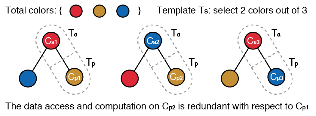
Figure 3. Identify the redundancy of Fascia color coding in a two-vertex sub-template $T_{s}$, which is further split into an active child and a passive child.

In Figure 3, we illustrate this redundancy by a $T_{s}$ with two colors taken out of three. Supposing $T_{s}$ has an active child $T_{s,a}$ with one color and a passive child $T_{s,p}$ with one color. The data access to $C_{s,p2}$ is redundant with respect to that of $C_{s,p1}$ because they share the same color of green. This redundant data access on passive children is non-trivial because it loops over all neighbors of $V_{i}$, where data locality is usually poor. Therefore, we develop a pruning technique in Section 4.1 to address this issue.

3.2. Lack of Vectorization and Data Locality

Although $M_{s}$ stores its values in a dense matrix, the index system of Equation 1 does not guarantee that the looping over $C_{s,a}$ and $C_{s,p}$ at line 8 of Algorithm 1 would have contiguous column indices at $M_{s,a}$ and $M_{s,p}$. For instance, in Figure 2, $I_{s,ca1}=1$, $I_{s,ca1}=0$ while $I_{s,ca3}=2$. Hence, the work by a thread on each row of $M_{s,a}$ and $M_{s,p}$ cannot be vectorized because of this irregular access pattern. Also, this irregular access pattern compromises the data locality of cache usage. For example, a cache line that prefetches a 64-Byte chunk from memory address starting at $\&M_{s,a}(1,1)$ and ending at $\&M_{s,a}(1,16)$ cannot serve the request to access $M_{s,a}(1,0)$. It is even harder to cache data access to $M_{s,p}$ because they belong to different rows (neighbor vertices). We shall address this issue by re-designing data structure and thread execution order in Section 4.2 to 4.4.

4. Design and Implementation

To resolve the performance issues in Section 3.1 and 3.2, we first identify and prune the unnecessary computation and memory access in Algorithm 1. Secondly, we modify the underlying data structure, the thread execution workflow, and provide a fully-vectorized implementation by using linear algebra kernels.

4.1. Pruning Color Combinations

To remove the redundancy observed in Section 3.1, we first apply the transformation by Equation 2 using the distributive property of addition and multiplication,

(2) $$\sum_{V_{j}\in N(i)}M_{s,a}(i,I_{s,a})\cdot M_{s,p}(j,I_{s,p})=M_{s,a}(i,I_{s,a})\sum_{V_{j}\in N(i)}M_{s,p}(j,I_{s,p})$$

where it adds up all the $M_{s,p}(j,I_{s,p})$ before multiplying $M_{s,a}(i,I_{s,a})$ while keeping the same arithmetic result. The implementation will be illustrated in detail in Figure 5.

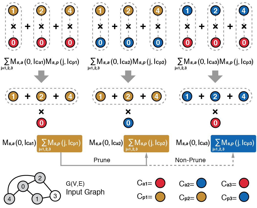
Figure 4. Illustrate steps of pruning optimization from vertex 0 in $G=(V,E)$ with the three color combinations shown in Figure 3. 1) Re-order addition and multiplication (grey arrow); 2): prune the vertex neighbor summation.

Secondly, we check whether multiple color combinations share the same $C_{s,p}$ and prune them by re-using the result from its first occurrence. In Figure 4, we examine a case with a sub-template $T_{s}$ choosing two colors out of three. In this case, $T_{s}$ is split into an active child $T_{s,a}$ with one vertex and a passive child $T_{s,p}$ with one vertex. Obviously, the neighbor traversal of vertex $V_{0}$ for $C_{s,a2},C_{s,p2}$ is pruned by using the results from $\{C_{s,a1},C_{s,p1}\}$.

4.2. Pre-compute Neighbor Traversal

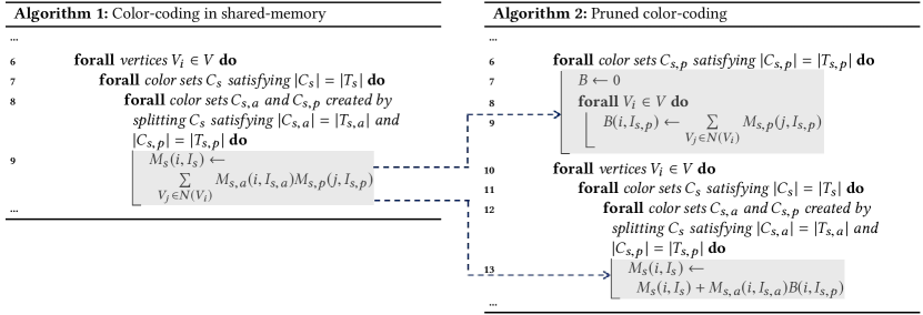
Figure 5. Pre-compute the pruned vertex-neighbor traversal by: 1) stripping out the summation of count data $M_{s,p}$ from its multiplication by count data from $M_{s,a}$; 2) storing the summation value of $M_{s,p}$ and looking it up before multiplying count data from $M_{s,a}$

Furthermore, the traversal of neighbors to sum up $M_{s,p}$ counts is stripped out from the for loop at line 2 of Algorithm 1 as a pre-computation module shown in Figure 4. We use an array buffer of length $|V|$ to temporarily hold the summation results for a certain $C_{s,p}$ across all $V_{i}$ with $SumBuf[i]=\sum_{V_{j}\in N(i)}M_{s,p}(j,I_{s,p})$. After the pre-computation for $C_{s,p}$, we write the content of buffer back to $M_{s,p}(V_{i},I_{s,p})$ and release $SumBuf$ for the next $C_{s,p}$. We then replace the calculations of $\sum_{V_{j}\in N(i)}M_{s,p}(j,I_{s,p})$ by looking up their values from $M_{s,p}(i,I_{s,p})$. Meanwhile, except for the $|V|$-sized array buffer, we do not increase the memory footprint for this pre-computation module.

It is worth noting that the pruning of vertex neighbor traversal shall also benefit the performance in a distributed memory system, where the data request to a vertex neighbor would be much expensive than that in a shared-memory system because of explicit interprocess communication.

4.3. Data Structure for Better Locality

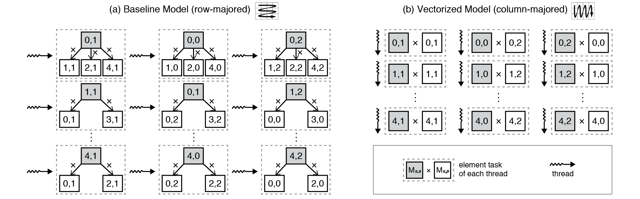
Figure 6. Comparing the thread execution order, where (a) Fascia color coding (baseline Model) has count data stored in memory with a row-majored layout, and (b) Pgbsc (Vectorized Model) has count data stored in memory with a column-majored layout.

We replace the adjacency list $adj[][]$ of network $G(V,E)$ by using an adjacency matrix $A_{G}$, where $A_{G}(i,j)=1$ if $V_{j}$ is a neighbor of $V_{i}$, and otherwise $A_{G}(i,j)=0$. The adjacency matrix has two advantages in our case:

1. It enables us to represent the neighbor vertex traversal at line 9 of Algorithm 2 by using a matrix operation.

2. It allows a pre-processing step upon the sparse matrix to improve the data locality of the network if necessary.

The pre-processing step would be quite efficient in processing an extremely large network with a high sparsity in a distributed-memory system. For example, the Reverse Cuthill-McKee Algorithm (RCM) reduces the communication overhead as well as improves the bandwidth utilization (Azad et al., 2017). Because the sparse matrix would be re-used by each vertex $V_{i}$, this additional pre-processing overhead is amortized and neglected in practice.

For count tables in $M[]$, we keep the dense matrices but change the data layout in physical memory from row-majored order in Figure 6(a) to column-majored order in Figure 6(b). The column-majored viewpoint reflects a vector form of count data, i.e., the count data for a certain color combination $C$ is stored in a $|V|$ dimensional vector, which is essential to our next vectorization effort, because all of the count data for a certain color combination $C$ from all vertices $V_{i}\in G(V,E)$ are now stored in contiguous memory space.

4.4. Vectorized Thread Execution and Memory Access

With the new locality-friendly data structure, we vectorize the counting tasks and memory access by re-ordering the thread execution workflow. Here the thread is created by users, e.g., we use OpenMP 4.0 to spawn threads.

To vectorize the pre-computation of $\sum_{V_{j}\in N(i)}M_{s,p}(j,w)$ for each vertex $V_{i}$, we extend the buffer in Section 3.1 from an $|V|$ dimensional array into a $|V|\times Z$ matrix $M_{buf}$, where $Z$ is a pre-selected batch size and data is stored in a row-majored order. We have the following procedure:

1. For each vertex $V_{i}$, load the first $Z$ values from row $M_{s,p}(i,:)$ into $M_{buf}(i,:)$.

2. All rows (vertices) of $M_{buf}$ are processed by threads in parallel.

3. For each row, a thread sequentially loops over $V_{j}\in N(i)$ to calculate $M_{s,p}(i,z)\leftarrow M_{s,p}(i,z)+M_{buf}(j,z)$.

The batch size value $Z$ shall be a multiple of the SIMD unit length or the cache line size, which ensures full utilization of the vector register length and the prefetched data in a cache line.

To vectorize the execution of count task at line 9 of Algorithm 1, we change the thread workflow from Figure 6(a) to Figure 6(b). In Figure 6(a), the Fascia color coding has each thread process counting work belonging to a vertex at a time. Conversely, in Figure 6(b), we characterize the thread workflow as:

1. Tasks belong to one color combination but for all vertices in $G(V,E)$, is dispatched altogether to all threads at a time. All threads collaboratively finish these tasks before moving to tasks for the next color combination.

2. For the tasks from the same color combination, each thread is assigned an equal portion of element tasks with consecutive row numbers in $M_{s,a}$ and $M_{s,p}$.

3. For each thread, within its portion of element tasks, the calculation is vectorized due to the consecutive row number and the column-majored data storage layout.

Typically $|V|$ has more than one million vertices in the network and is much larger than the total thread number. Each thread gets a portion of tasks much larger than the SIMD unit length and ensures full utilization of its SIMD resource. Furthermore, regular stride 1 memory access of each thread on $M_{s,a}$ and $M_{s,p}$ enables an efficient data prefetching from memory into cache lines.

4.5. Exploit Linear Algebra Kernels

According to the GraphBLAS philosophy, the looping over a vertex’s neighbors is represented as a multiplication of a vector by the adjacency matrix. Therefore, the looping of neighbors for each $V_{i}\in V$ for pre-computing $M_{s,p}$ at line 8,9 of Algorithm 2 is written as $A_{G}M_{s,p}(:,I_{s,p})$ at line 4 of Algorithm 3, where $A_{G}$ is the adjacency matrix notated in Section 4.3 and $I_{s,p}$ is the column index for a color set $C_{s,p}$ in $M_{s,p}$. Such multiplication is identified as Sparse Matrix-Vector multiplication (SpMV). To save memory space, we store the multiplication result back to $M_{s,p}(:,I_{s,p})$ with the help of a buffer. In practice, our Pgbsc adopts a Compressed Sparse Column (CSC) format on $A_{G}$ and the looping over color sets $C_{s,p}$ to do SpMV at line 3,4 in Algorithm 3 is combined with a sparse matrix dense matrix (SpMM) kernel to apply the vectorization in Algorithm 4.

The vectorized counting task is implemented by an element-wise vector-vector multiplication and addition (named as eMA) kernel at line 7 of Algorithm 4, where vector $M_{s}(:,I_{c})$, $M_{s,a}(:,I_{s,a})$, and $M_{s,p}(:,I_{s,p})$ are retrieved from $M_{s}$, $M_{s,a}$, and $M_{s,p}$, respectively. We code this kernel by using Intel (R) AVX intrinsics, where multiplication and addition are implemented by using fused multiply-add (FMA) instruction set that leverages the 256/512-bit vector registers.

5. Complexity Analysis

In this section, we will first analyze the time complexity of the Pgbsc algorithm to show a significant reduction. Then, we will give the formula to estimate the improvement of Pgbsc versus Fascia.

5.1. Time Complexity

We assume that the size of the sub-templates is uniformly distributed between $1$ and $n$. We will use two matrix/vector operations, sparse matrix dense matrix multiplication (SpMM) and element-wise multiplication and addition (eMA). The time complexity of SpMV is considered as $|E|$, and the time complexity of eMA is $|V|$.

Lemma 5.1.

For a template or a sub-template $T_{s}$, if the counting of the sub-templates of $T_{s}$ has been completed, then the time complexity of counting $T_{s}$ is:

(3) $$O(|E|\binom{|T|}{|T_{s,p}|}+|V|\binom{|T|}{|T_{s}|}\binom{|T_{s}|}{|T_{s,p}|}).$$

Proof.

Since $T_{s,p}$ has $\binom{|T|}{|T_{s,p}|}$ color combinations, which requires $\binom{|T|}{|T_{s,p}|}$ times SpMV operations. The total time consumption of this step is $O(|E|\binom{|T|}{|T_{s,p}|})$. In the next step, $T_{s}$ has a total of $\binom{|T|}{|T_{s}|}$ different color combinations, and its sub-templates have a total of $\binom{|T_{s}|}{|T_{s,p}|}$ color combinations, a two-layer loop is needed here. The total time consumption of this step is $O(|V|\binom{|T|}{|T_{s}|}\binom{|T_{s}|}{|T_{s,p}|})$. ∎

Lemma 5.2.

For integers $l\leq m\leq n$, and $l_{0}\leq 0,l_{1}\leq 1,\dots,l_{n}\leq n,$ the following equations hold:

1. $\max_{m}\binom{n}{m}=O(n^{-1/2}2^{n})$

2. $\max_{\{m,l\}}\binom{n}{m}\binom{m}{l}=O(n^{-1}3^{n})$

3. $\max_{\{l_{0},l_{1},\dots,l_{n}\}}\sum_{m=0}^{n}\binom{n}{m}\binom{m}{l_{m}}=O(n^{-1/2}3^{n})$

Lemma 5.3.

In the worst case, the total time complexity of counting a $k$-node template using Pgbsc is

(4) $$O((e^{k}\log{(\frac{1}{\delta})}\frac{1}{\epsilon^{2}})(|E|2^{k}+|V|k^{-1/2}3^{k})).$$

Proof.

A template with $k$ nodes generates up to $O(k)$ sub-templates. And $O(e^{k}\log{(\frac{1}{\delta}})\frac{1}{\epsilon^{2}})$ iterations are performed in order to get the $(\epsilon,\delta)$-approximation. The conclusion is proved by combining Lemma 5.2. ∎

Table 2. Comparison with Original Subgraph Counting

Time complexity	One sub-template	One iteration
Fascia	$O(|E|\binom{|T|}{|T_{s}|}\binom{|T_{s}|}{|T_{s,p}|})$	$O(|E|\cdot k^{-1/2}3^{k})$
Pfascia	$O(|E|\binom{|T|}{|T_{s,p}|}+$ $|V|(\binom{|T|}{|T_{s}|}\binom{|T_{s}|}{|T_{s,p}|}+\binom{|T|}{|T_{s,p}|}))$	$O(|E|2^{k}+|V|k^{-1/2}3^{k}$)
Pgbsc	$O(|E|\binom{|T|}{|T_{s,p}|}+$ $|V|\binom{|T|}{|T_{s}|}\binom{|T_{s}|}{|T_{s,p}|})$	$O(|E|2^{k}+|V|k^{-1/2}3^{k})$

5.2. Estimation of Performance Improvement

In this section, we present a model to estimate the run time of Pgbsc and its improvement over the original algorithm.

Run time

From the previous analysis, we know that the execution time of Pgbsc on a single sub-template is $O(|E|\binom{|T|}{|T_{s,p}|}+|V|\binom{|T|}{|T_{s}|}\binom{|T_{s}|}{|T_{s,p}|})$. By supplementing the constant term, we get

(5) $$runtime_{PGBSC}=\alpha|E|\binom{|T|}{|T_{s,p}|}+\beta|V|\binom{|T|}{|T_{s}|}\binom{|T_{s}|}{|T_{s,p}|},$$

where $\alpha$ and $\beta$ are constants, and we will calculate them by applying the data fitting. Similarly, we set:

(6) $$runtime_{FASCIA}=\gamma|E|\binom{|T|}{|T_{s}|}\binom{|T_{s}|}{|T_{s,p}|}.$$

Through the previous research we obtained that the time complexity of the original color-coding algorithm and Pgbsc are $O(|E|k^{-1/2}3^{k})$ and $O(|E|2^{k}+|V|k^{-1/2}3^{k})$ respectively. Since the $|E|2^{k}$ term is very close to the actual value, and the $k^{-1/2}3^{k}$ term may be overestimated, to be more rigorous, we assume that the actual running time of the two programs is $|E|f(T)$ and $|E|2^{k}+|V|f(T)$ respectively. Here $T$ is the input template, and $f$ is a function for $T$. According to previous analysis, we obtain an upper bound of $f$: $O(f(T))\leq O(k^{-1/2}3^{k})$. The lower bound of $f(T)$ is estimated in this form:

(7) $$f(T)=\sum_{T_{s}}{\binom{|T|}{|T_{s}|}\binom{|T_{s}|}{|T_{s}|}}\geq\sum_{T_{s}}\binom{|T|}{|T_{s}|}|T_{s}|\approx\sum_{i}i\binom{k}{i}=n\cdot 2^{k-1}$$

Thus, $O(k\cdot 2^{k})\leq O(f(T))\leq O(k^{-1/2}3^{k})$. Comparing the complexity of the two algorithms we obtain: $Improvement\approx\frac{\gamma|E|f(T)}{\alpha|E|2^{k}+\beta|V|f(T)}=\frac{\gamma}{\alpha\frac{2^{k}}{f(T)}+\beta|V|/|E|}=\frac{\gamma}{\alpha\frac{2^{k}}{f(T)}+\beta d^{-1}}.$

Since the influence of the constant term is not considered in the complexity analysis, we need to fill in the necessary constant terms:

(8) $$\gamma(\alpha\cdot 2\cdot k^{-1}+\beta\cdot d^{-1})^{-1}\leq Improvement\leq\gamma(\alpha\cdot(\frac{2}{3})^{k}+\beta\cdot d^{-1})^{-1},$$

where $d$ is the average degree of the network, $\alpha$, $\beta$,and $\gamma$ are constants.

For a given graph, the following implications are obtained from this formula:

1. The improvement grows with increasing template size, but no more than an upper bound, which is $\gamma\beta^{-1}d$.

2. For a relatively small average degree $d$, the improvement is proportional to $d$, and the ratio is $\gamma\beta^{-1}$.

3. For a relatively large average degree $d$, improvement will approach an upper bound between $\gamma\alpha^{-1}k$ and $\gamma\alpha^{-1}(\frac{3}{2})^{k}$.

6. Experimental Setup

6.1. Software

We use the following three implementations. All of the binaries are compiled by the Intel(R) C++ compiler for Intel(R) 64 target platform from Intel(R) Parallel Studio XE 2019, with compilation flags of “-O3“, “-xCore-AVX2”, “-xCore-AVX512”, and the Intel(R) OpenMP.

• Fascia implements the FASCIA algorithm in (Slota and Madduri, 2013), which serves as a performance baseline.

• PFascia implements the data structure of Fascia but applying a pruning optimization on the graph traversal.

• Pgbsc implements both of pruning optimization and the GraphBLAS inspired vectorization.

6.2. Datasets and Templates

Figure 7. Templates used in experiments

The datasets in our experiments are listed in Table 3, where Graph500 Scale=20, 21, 22 are collected from (GraphChallenge, 2019); Miami, Orkut, and NYC are from  (Barrett et al., 2009) (Leskovec and Krevl, 2014) (Yang and Leskovec, 2012); RMAT are widely used synthetic datasets generated by the RMAT model (Chakrabarti et al., 2004). The templates in Figure 7 are from the tests in (Slota and Madduri, 2013) or created by us. The template size increases from 10 to 17 while some templates have two different shapes.

Table 3. Datasets used in the experiments (K=$10^{3}$, M=$10^{6}$)

Data	Vertices	Edges	Avg Deg	Max Deg	Abbreviation	Source
Graph500 Scale=20	600K	31M	48	67K	GS20	Graph500 (GraphChallenge, 2019)
Graph500 Scale=21	1M	63M	51	107K	GS21	Graph500 (GraphChallenge, 2019)
Graph500 Scale=22	2M	128M	53	170K	GS22	Graph500 (GraphChallenge, 2019)
Miami	2.1M	200M	49	10K	MI	Social network (Barrett et al., 2009)
Orkut	3M	230M	76	33K	OR	Social network (Leskovec and Krevl, 2014)
NYC	18M	960M	54	429	NY	Social network (Yang and Leskovec, 2012)
RMAT-1M	1M	200M	201	47K	RT1M	Synthetic data (Chakrabarti et al., 2004)
RMAT(k=3)	4M	200M	52	26K	RTK3	Synthetic data (Chakrabarti et al., 2004)
RMAT(k=5)	4M	200M	73	144K	RTK5	Synthetic data (Chakrabarti et al., 2004)
RMAT(k=8)	4M	200M	127	252K	RTK8	Synthetic data (Chakrabarti et al., 2004)

6.3. Hardware

In the experiments, we use: 1) a single node of a dual-socket Intel(R) Xeon(R) CPU E5-2670 v3 (architecture Haswell), and 2) a single node of a dual-socket Intel(R) Xeon(R) Platinum 8160 CPU (architecture Skylake-SP) processors.

Table 4. Node Specification of Testbed

Arch	Sockets	Cores	Threads	CPU Freq	Peak Performance
Haswell	2	24	48	2.3GHz	1500 GFLOPS
Skylake	2	48	96	2.1GHz	4128 GFLOPS
Arch	L1(i/d)	L2	L3	Memory Size	Memory Bandwidth
Haswell	32KB	256KB	30MB	125GB	95GB/s
Skylake	32KB	1024KB	33MB	250GB	140GB/s

The Operating System is Red Hat Enterprise Linux Server version 7.6 for both of the nodes, whose specifications are shown in Table 4. We use Haswell and Skylake to refer to the Intel(R) Xeon(R) CPU E5-2670 v3 and Intel(R) Xeon(R) Platinum 8160 CPU respectively in the rest of the paper. The memory bandwidth is measured by STREAME Benchmark (McCalpin et al., 1995) while the peak performance is measured by using the Intel(R) Optimized LINPACK Benchmark for Linux. We use, by default, the number of threads equal to the number of physical cores, i.e., 48 threads on Skylake node and 24 threads on Haswell node. The threads are bound to cores with a spread affinity. As the Skylake node has twice the memory size and physical cores as the Haswell node, we use it as our primary testbed in the experiments.

7. Performance and Hardware Utilization

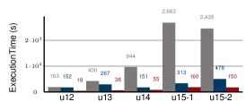
(a) Miami

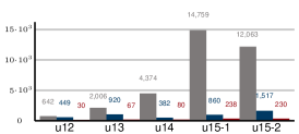
(b) Orkut

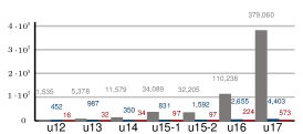
(c) RMAT-1M

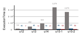
(d) Graph500 Scale=20

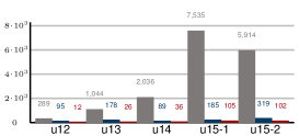
(e) Graph500 Scale=21

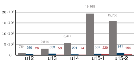
(f) Graph500 Scale=22

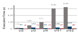
(g) RMAT K=3

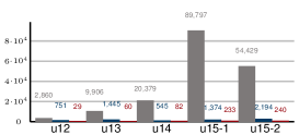
(h) RMAT K=5

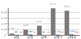
(i) RMAT K=8

Figure 8. Execution time of Fascia  versus PFascia versus Pgbsc with increasing template sizes, from U12 to U17. Tests run on a Skylake node.

In Figure 8(a)(b)(c), we scale the template size up to the memory limitation of our testbed for each dataset, and the reduction of execution time is significant particularly for template sizes larger than 14. For instance, Fascia spends four days to process a million-vertex dataset RMAT-1M with template u17 while Pgbsc only spends 9.5 minutes. For relatively smaller templates such as u12, Pgbsc still achieves 10x to 100x the reduction of execution time on datasets Miami, Orkut, and RMAT-1M. As discussed in Section 5.2, the improvement is proportional to its average degree. This is observed when comparing datasets Miami (average degree of 49) and Orkut (average degree of 76), where Pgbsc achieve 10x and 20x improvement on u12 respectively. In Figure 8(d)(e)(f), we scale up the size of Graph500 datasets in Table 3. Note that all of the Graph500 datasets have similar average degrees and get similar improvement by Pgbsc for the same template. This implies that Pgbsc delivers the same performance boost to datasets with a comparable average degree but different scales. Finally, in Figure 8(g)(h)(i), we compare RMAT datasets with increasing skewness, which causes the imbalance of vertex degree distribution. The results show that Pgbsc has comparable execution time regardless of the growing degree distribution skewness. In contrast, Fascia spends significantly (2x to 3x) more time on skewed datasets. To validate the performance gained by using Pgbsc, we investigate the performance improvement contributed by pruning and vectorization, accordingly to Section 7.1 and 7.2.

7.1. Pruning Optimization

In Figure 9, we compare six datasets with each starting from the template u12 and up to the largest templates whose count data the Skylake node can hold. Three observations are made: 1) PFascia achieves a performance improvement of 10x by average and up to 86x. 2) PFascia obtains higher relative performance on large templates. For instance, it gets 17.2x improvement for u15-1 while only 2.2x for u13 for dataset Orkut. 3) PFascia works better at datasets with high skewness of degree distribution. Datasets like Miami and Orkut that have a power law distribution only get 8.5x and 17.2x improvement at u15-1, while the RMAT-1M obtains 41x improvement.

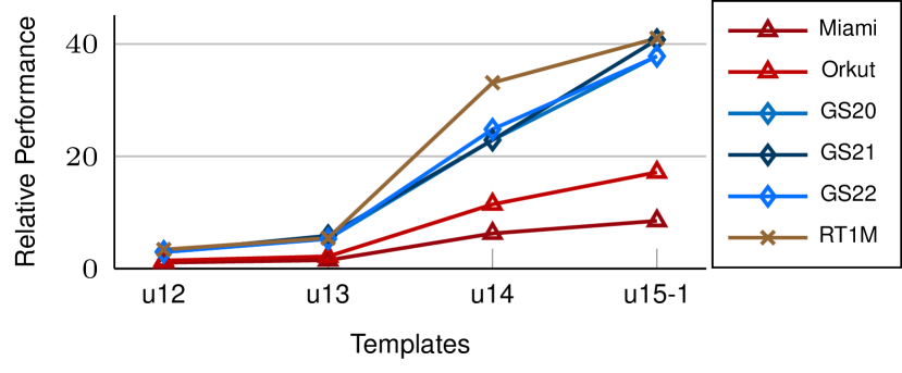
Figure 9. Relative performance of PFascia versus Fascia with increasing template sizes. Tests are done on a Skylake node.

7.2. Vectorization Optimization

We decompose Pgbsc into the two linear algebra kernels SpMM and eMA as described in Section 4.5.

7.2.1. CPU and VPU Utilization

Figure 10(a) first compares the CPU utilization defined as the average number of concurrently running physical cores. For Miami, PFascia and Fascia achieve 60% and 75% of CPU utilization. However, the CPU utilization drops below 50% on Orkut and NYC who have more vertices and edges than Miami. Conversely, SpMM kernel keeps a high ratio of 65% to 78% for all three of the datasets, and the eMA kernel has a growing CPU utilization from Miami (46%) to NYC (88%). We have two explanations: 1) the SpMM kernel splits and regroups the nonzero entries by their row IDs, which mitigates the imbalance of nonzero entries among rows; 2) the eMA kernel has its computation workload for each column of $M_{s,a},M_{s,p}$ evenly dispatched to threads.

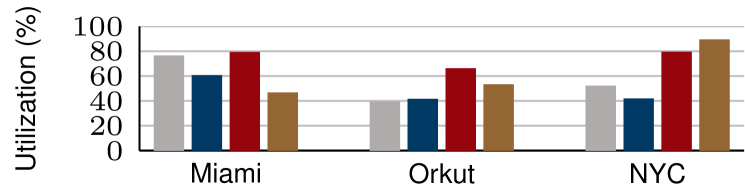
(a) CPU Utilization

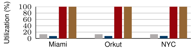
(b) VPU Utilization

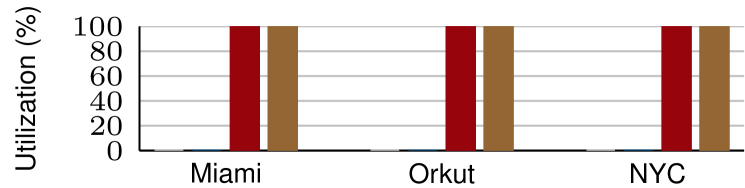
(c) Packed FP

Figure 10. The hardware utilization on Skylake node for template u12.

Secondly, we examine the code vectorization in Figure 10. VPU in a Skylake node is a group of 512-bit registers. The scalar instruction also utilizes the VPU but it cannot fully exploit its 512-bit length. Figure 10 refers to the portion of instructions vectorized with full vector capacity. For all of the three datasets, PFascia and Fascia only have 6.7% and 12.5% VPU utilization implying that the codes may not be vectorized, while for SpMM and eMA kernels of Pgbsc, the VPU utilization is 100%. A further metric of packed float point instruction ratio (Packed FP) justifies the implication that PFascia and Fascia have zero vectorized instructions but Pgbsc has all of its float point operations vectorized.

7.2.2. Memory Bandwidth and Cache

Because of the sparsity, subgraph counting is memory-bounded in a shared memory system. Therefore, the utilization of memory and cache resources are critical to the overall performance. In Table 5, we compare SpMM and eMA of to PFascia and Fascia. It shows that the eMA kernel has the highest bandwidth value around 110 GB/s for the three datasets, which is due to the highly vectorized codes and regular memory access pattern. Therefore, the data is prefetched into cache lines, which controls the cache miss rate as low as 0.1%.

The SpMM kernel also enjoys a decent bandwidth usage around 70 to 80 GB/s by average when compared to PFascia and Fascia. Although SpMM has an L3 miss rate as high as 74% in dataset NYC because the dense matrix is larger than the L3 cache capacity. The optimized thread level and instruction level vectorization ensures a concurrent data loading from memory leveraging the high memory bandwidth utilization. Fascia has the lowest memory bandwidth usage because of the thread imbalance and the irregular memory access.

Table 5. Memory and Cache Usage on Skylake Node

Miami	Bandwidth	L1 Miss Rate	L2 Miss Rate	L3 Miss Rate
FASCIA	6 GB/s	4.1%	1.8%	85%
PFASCIA	48.8 GB/s	9.5%	86.5%	50%
PGBSC-SpMM	86.95 GB/s	8.3%	51.2%	36.8%
PGBSC-eMA	106 GB/s	0.3%	20.6%	9.9%
Orkut	Bandwidth	L1 Miss Rate	L2 Miss Rate	L3 Miss Rate
FASCIA	8 GB/s	9.6%	5.3%	46%
PFASCIA	30 GB/s	8.4%	76.2%	46%
PGBSC-SpMM	59.5 GB/s	6.7%	42.8%	45%
PGBSC-eMA	116 GB/s	0.32%	22.2%	9.0%
NYC	Bandwidth	L1 Miss Rate	L2 Miss Rate	L3 Miss Rate
FASCIA	7 GB/s	2.4%	8.1%	87%
PFASCIA	38 GB/s	10%	90%	81%
PGBSC-SpMM	96 GB/s	7.7%	76%	74%
PGBSC-eMA	122 GB/s	0.1%	99%	14.8%

7.2.3. Roofline Model

The roofline model in Figure 11 reflects the hardware efficiency. The horizontal axis is the operational intensity (FLOP/byte) and the vertical axis refers to the measured throughput performance (FLOP/second). The solid roofline is the maximal performance the hardware can deliver under a certain operational intensity. From Fascia to PFascia, the performance gap to the roofline grows, implying that the pruning optimization itself does not improve the hardware utilization although it removes redundant computation. From PFascia to Pgbsc, the performance gap to the roofline is reduced significantly, resulting in a performance point hit by the roofline. This near-full hardware efficiency is contributed by the vectorization optimization, which exploits the memory bandwidth usage.

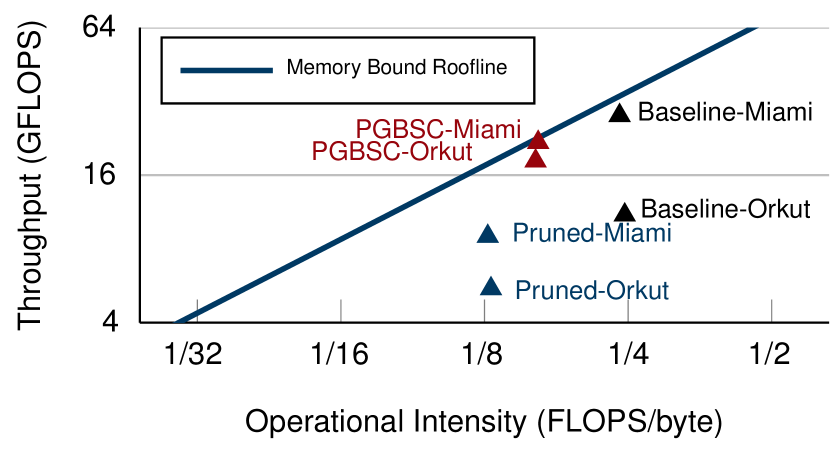
Figure 11. Apply roofline model to Fascia, PFascia,and Pgbsc. Dataset Miami, Orkut for template u15-1. Tests are done on a Skylake node.

Figure  12 compares the performance of Pgbsc between the Skylake node and the Haswell node. For both test beds, we set up threads numbered equal to their physical cores, and Skylake node in has a 1.7x improvement over Haswell node. Although the Skylake node doubles the CPU cores compared to the Haswell node, it increases the peak memory bandwidth by only 47% in Table 4. As Pgbsc is bounded by the memory roofline in Figure 11, the estimated improvement shall be a value between 1.47x and 2x, and the $1.7x$ improvement by Pgbsc is reasonable.

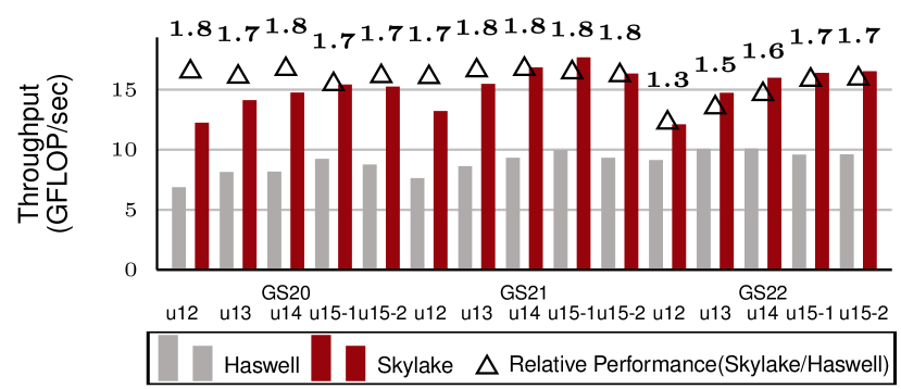
Figure 12. The performance throughput of Pgbsc on Haswell node versus. Skylake node.

7.3. Load Balance and Thread Scaling

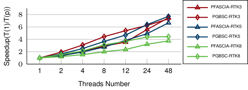
Figure 13. Thread scaling for RMAT datasets with increasing skewness on a Skylake node.

We perform a strong scaling test using up to 48 threads on Skylake node in Figure 13. We choose RMAT generated datasets with increasing skewness parameters of $K=3,5,8$. When $K=3$, Pgbsc has a better thread scaling than PFascia from 1 to 12 threads; after 12 threads, the thread scaling of Pgbsc slows down. As the performance is bounded by memory, which has 6 memory channels per socket, we have a total of 12 memory channels on a Skylake node that bounds the thread scaling. To the contrary, PFascia is not bounded by the memory bandwidth, which explains why it keeps an increasing thread scaling from 12 to 48 threads. Eventually, both of Pgbsc and PFascia obtain a 7.5x speedup at 48 threads. When increasing the skewness of datasets to $K=5,8$, the thread scalability of PFascia and Pgbsc both drop down because the skewed data distribution brings workload imbalance when looping vertex neighbors. However, Pgbsc has a better scalability than PFascia at 48 threads because of the SpMM kernel.

7.4. Error Discussion

Pgbsc with its pruning and vectorization optimization only differs from the Fascia due to the restructuring of the computation from Algorithm 1 to Algorithm 4, and so should give identical results with exact arithmetic in Equation 2. However,the range of values needed when processing large templates. As a consequence, both Fascia and our Pgbsc use floating point numbers to avoid overflow. Hence, slightly different results are observed between Fascia and Pgbsc due to the rounding error consequent from floating point arithmetic operations. Figure 14 reports such relative error in the range of $10^{-6}$ across all the tests on a Graph500 GS20 dataset with increasing template sizes, which is negligible.

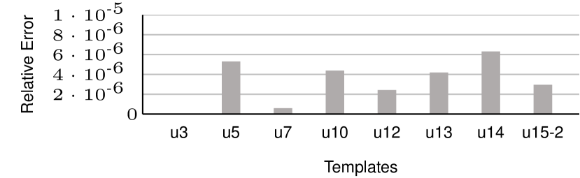
Figure 14. Relative error on dataset Graph500 Scale=20. Tests are done on a Skylake node.

7.5. Overall Performance Improvement

Figure 15 shows significant performance improvement of Pgbsc over Fascia for a variety of networks and subtemplates; the relative performance grows with template sizes.

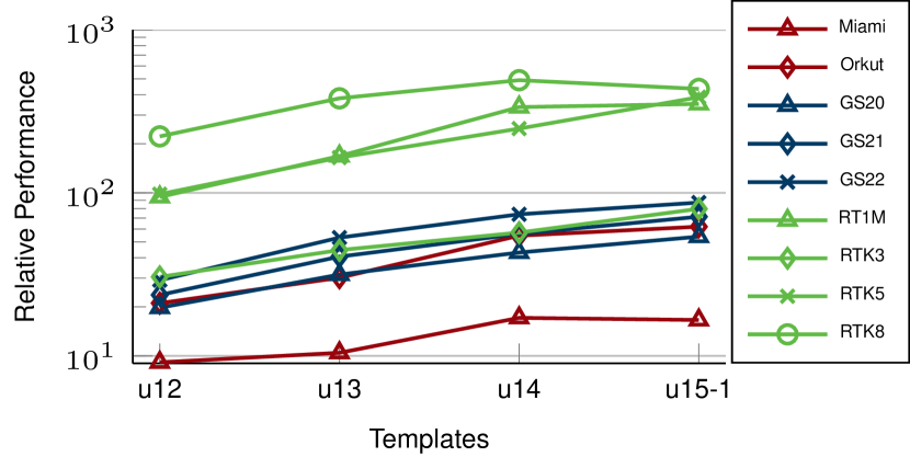
Figure 15. Performance improvement of Pgbsc vs. Fascia with increasing template sizes. Tests are done on a Skylake node.

For small dataset Miami and template u12, they still achieve 9x improvement, and for datasets like Graph500 (scale:20) and templates with size starting from u14, Pgbsc achieves around 50x improvement by average and up to 660x improvement for synthetic dataset RT1M at large template u17.

8. Conclusion

As the single machine with big shared memory and many cores is becoming an attractive solution to graph analysis problems (Perez et al., 2015), the irregularity of memory access remains a roadblock to improve hardware utilization. For fundamental algorithms, such as PageRank, the fixed data structure and predictable execution order are explored to improve data locality either in graph traversal approach  (Lakhotia et al., 2017)(Zhang et al., 2017) or in linear algebra approach (Beamer et al., 2017). Subgraph counting, with random access to vast memory region and dynamic programming workflow, requires much more effort to exploit the cache efficiency and hardware vectorization. To the best of our knowledge, we are the first to fully vectorize a sophisticated algorithm of subgraph analysis, and the novelty is a co-design approach to combine algorithmic improvement with pattern identification of linear algebra kernels that leverage hardware vectorization.

The overall performance achieves a promising improvement over the state-of-the-art work by orders of magnitude by average and up to 660x (RMAT1M with u17) within a shared-memory multi-threaded system, and we are confident to generalize this GraphBLAS inspired approach in our future work: 1) enabling counting of tree subgraph with size larger than 30 and subgraph beyond trees; 2) extending the shared-memory implementation to distributed system upon our prior work (Chen et al., 2018) (Slota and Madduri, 2014)  (Zhao et al., 2018) (Zhao et al., 2012); 3) exploring other graph and machine learning problems by this GraphBLAS inspired co-design approach; 4) adding support to more hardware architectures (e.g, NEC SX-Aurora and NVIDIA GPU). The codebase of our work on Pgbsc is made public in our open-sourced repository.

9. Acknowledgments

We gratefully acknowledge generous support from the Intel Parallel Computing Center (IPCC), the NSF CIF-DIBBS 1443054: Middleware and High-Performance Analytics Libraries for Scalable Data Science, and NSF BIGDATA 1838083: Enabling Large-Scale, Privacy-Preserving Genomic Computing with a Hardware-Assisted Secure Big-Data Analytics Framework. We appreciate the support from the IU PHI grand challenge, the FutureSystems team, and the ISE Modelling and Simulation Lab.

References

- (1)
- Ahmed et al. (2015) Nesreen K Ahmed, Jennifer Neville, Ryan A Rossi, and Nick Duffield. 2015. Efficient graphlet counting for large networks. In Data Mining (ICDM), 2015 IEEE International Conference on. IEEE, 1–10.
- Alon et al. (2008) Noga Alon, Phuong Dao, Iman Hajirasouliha, Fereydoun Hormozdiari, and S Cenk Sahinalp. 2008. Biomolecular network motif counting and discovery by color coding. Bioinformatics 24, 13 (2008), i241–i249.
- Alon and Gutner (2007) Noga Alon and Shai Gutner. 2007. Balanced families of perfect hash functions and their applications. In International Colloquium on Automata, Languages, and Programming. Springer, 435–446.
- Alon et al. (1995) Noga Alon, Raphael Yuster, and Uri Zwick. 1995. Color-coding. Journal of the ACM (JACM) 42, 4 (1995), 844–856.
- Arvind and Raman (2002) Vikraman Arvind and Venkatesh Raman. 2002. Approximation algorithms for some parameterized counting problems. In International Symposium on Algorithms and Computation. Springer, 453–464.
- Azad et al. (2015) A. Azad, A. Buluç, and J. Gilbert. 2015. Parallel Triangle Counting and Enumeration Using Matrix Algebra. In 2015 IEEE International Parallel and Distributed Processing Symposium Workshop (2015-05). 804–811. https://doi.org/10.1109/IPDPSW.2015.75
- Azad et al. (2017) Ariful Azad, Mathias Jacquelin, Aydin Buluç, and Esmond G Ng. 2017. The reverse Cuthill-McKee algorithm in distributed-memory. In Parallel and Distributed Processing Symposium (IPDPS), 2017 IEEE International. IEEE, 22–31.
- Azad et al. (2018) Ariful Azad, Georgios A Pavlopoulos, Christos A Ouzounis, Nikos C Kyrpides, and Aydin Buluç. 2018. HipMCL: a high-performance parallel implementation of the Markov clustering algorithm for large-scale networks. Nucleic acids research 46, 6 (2018), e33–e33.
- Barrett et al. (2009) Christopher L Barrett, Richard J Beckman, Maleq Khan, VS Anil Kumar, Madhav V Marathe, Paula E Stretz, Tridib Dutta, and Bryan Lewis. 2009. Generation and analysis of large synthetic social contact networks. In Winter Simulation Conference. Winter Simulation Conference, 1003–1014.
- Beamer et al. (2017) Scott Beamer, Krste Asanović, and David Patterson. 2017. Reducing PageRank communication via propagation blocking. In Parallel and Distributed Processing Symposium (IPDPS), 2017 IEEE International. IEEE, 820–831.
- Bressan et al. (2017) Marco Bressan, Flavio Chierichetti, Ravi Kumar, Stefano Leucci, and Alessandro Panconesi. 2017. Counting graphlets: Space vs time. In Proceedings of the Tenth ACM International Conference on Web Search and Data Mining. ACM, 557–566.
- Buluç and Gilbert (2011) Aydın Buluç and John R Gilbert. 2011. The Combinatorial BLAS: Design, implementation, and applications. The International Journal of High Performance Computing Applications 25, 4 (2011), 496–509.
- Chakaravarthy et al. (2016) Venkatesan T Chakaravarthy, Michael Kapralov, Prakash Murali, Fabrizio Petrini, Xinyu Que, Yogish Sabharwal, and Baruch Schieber. 2016. Subgraph counting: Color coding beyond trees. In Parallel and Distributed Processing Symposium, 2016 IEEE International. Ieee, 2–11.
- Chakrabarti et al. (2004) Deepayan Chakrabarti, Yiping Zhan, and Christos Faloutsos. 2004. R-MAT: A recursive model for graph mining. In Proceedings of the 2004 SIAM International Conference on Data Mining. SIAM, 442–446.
- Chen et al. (2018) Langshi Chen, Bo Peng, Sabra Ossen, Anil Vullikanti, Madhav Marathe, Lei Jiang, and Judy Qiu. 2018. High-Performance Massive Subgraph Counting Using Pipelined Adaptive-Group Communication. Big Data and HPC: Ecosystem and Convergence 33 (2018), 173.
- Chen and Lui (2018) Xiaowei Chen and John Lui. 2018. Mining graphlet counts in online social networks. ACM Transactions on Knowledge Discovery from Data (TKDD) 12, 4 (2018), 41.
- Davis (2018) Timothy A Davis. 2018. Graph algorithms via SuiteSparse: GraphBLAS: triangle counting and K-truss. In 2018 IEEE High Performance extreme Computing Conference (HPEC). IEEE, 1–6.
- Ekanayake et al. (2018) Saliya Ekanayake, Jose Cadena, Udayanga Wickramasinghe, and Anil Vullikanti. 2018. MIDAS: Multilinear Detection at Scale. In 2018 IEEE International Parallel and Distributed Processing Symposium (IPDPS). IEEE, 2–11.
- GraphChallenge (2019) GraphChallenge. 2019. Graph Challenge MIT. https://graphchallenge.mit.edu/data-sets
- Hutchison et al. (2016) Dylan Hutchison, Jeremy Kepner, Vijay Gadepally, and Bill Howe. 2016. From NoSQL Accumulo to NewSQL Graphulo: Design and utility of graph algorithms inside a BigTable database. In High Performance Extreme Computing Conference (HPEC), 2016 IEEE. IEEE, 1–9.
- Kepner et al. (2016) Jeremy Kepner, Peter Aaltonen, David Bader, Aydın Buluç, Franz Franchetti, John Gilbert, Dylan Hutchison, Manoj Kumar, Andrew Lumsdaine, Henning Meyerhenke, et al. 2016. Mathematical foundations of the GraphBLAS. arXiv preprint arXiv:1606.05790 (2016).
- Kepner et al. (2015) Jeremy Kepner, David Bade, Aydın Buluç, John Gilbert, Timothy Mattson, and Henning Meyerhenke. 2015. Graphs, matrices, and the GraphBLAS: Seven good reasons. arXiv preprint arXiv:1504.01039 (2015).
- Lakhotia et al. (2017) Kartik Lakhotia, Rajgopal Kannan, and Viktor Prasanna. 2017. Accelerating PageRank using Partition-Centric Processing. (2017).
- Leskovec and Krevl (2014) Jure Leskovec and Andrej Krevl. 2014. SNAP Datasets: Stanford Large Network Dataset Collection. http://snap.stanford.edu/data.
- Mattson et al. (2013) Tim Mattson, David Bader, Jon Berry, Aydin Buluc, Jack Dongarra, Christos Faloutsos, John Feo, John Gilbert, Joseph Gonzalez, Bruce Hendrickson, et al. 2013. Standards for graph algorithm primitives. In 2013 IEEE High Performance Extreme Computing Conference (HPEC). IEEE, 1–2.
- Mattson et al. (2017) Timothy G Mattson, Carl Yang, Scott McMillan, Aydin Buluç, and José E Moreira. 2017. GraphBLAS C API: Ideas for future versions of the specification. In High Performance Extreme Computing Conference (HPEC), 2017 IEEE. IEEE, 1–6.
- McCalpin et al. (1995) John D McCalpin et al. 1995. Memory bandwidth and machine balance in current high performance computers. IEEE computer society technical committee on computer architecture (TCCA) newsletter 1995 (1995), 19–25.
- Perez et al. (2015) Yonathan Perez, Rok Sosič, Arijit Banerjee, Rohan Puttagunta, Martin Raison, Pararth Shah, and Jure Leskovec. 2015. Ringo: Interactive graph analytics on big-memory machines. In Proceedings of the 2015 ACM SIGMOD International Conference on Management of Data. ACM, 1105–1110.
- Pržulj (2007) Nataša Pržulj. 2007. Biological network comparison using graphlet degree distribution. Bioinformatics 23, 2 (2007), e177–e183.
- Rahman et al. (2014) Mahmudur Rahman, Mansurul Alam Bhuiyan, and Mohammad Al Hasan. 2014. Graft: An efficient graphlet counting method for large graph analysis. IEEE Transactions on Knowledge and Data Engineering 26, 10 (2014), 2466–2478.
- Reza et al. (2018) Tahsin Reza, Matei Ripeanu, Nicolas Tripoul, Geoffrey Sanders, and Roger Pearce. 2018. PruneJuice: pruning trillion-edge graphs to a precise pattern-matching solution. In Proceedings of the International Conference for High Performance Computing, Networking, Storage, and Analysis. IEEE Press, 21.
- Slota and Madduri (2013) George M Slota and Kamesh Madduri. 2013. Fast approximate subgraph counting and enumeration. In Parallel Processing (ICPP), 2013 42nd International Conference on. IEEE, 210–219.
- Slota and Madduri (2014) George M Slota and Kamesh Madduri. 2014. Complex network analysis using parallel approximate motif counting. In Parallel and Distributed Processing Symposium, 2014 IEEE 28th International. IEEE, 405–414.
- Sundaram et al. (2015) Narayanan Sundaram, Nadathur Satish, Md Mostofa Ali Patwary, Subramanya R. Dulloor, Michael J. Anderson, Satya Gautam Vadlamudi, Dipankar Das, and Pradeep Dubey. 2015. GraphMat: High Performance Graph Analytics Made Productive. Proceedings of the VLDB Endowment 8, 11 (2015), 1214–1225. https://doi.org/10.14778/2809974.2809983
- Yang et al. (2018) Carl Yang, Aydin Buluc, and John D. Owens. 2018. Design Principles for Sparse Matrix Multiplication on the GPU. (2018).
- Yang and Leskovec (2012) Jaewon Yang and Jure Leskovec. 2012. Defining and evaluating network communities based on ground-truth. Knowledge & Information Systems 42, 1 (2012), 181–213.
- Zhang et al. (2016) P. Zhang, M. Zalewski, A. Lumsdaine, S. Misurda, and S. McMillan. 2016. GBTL-CUDA: Graph Algorithms and Primitives for GPUs. In 2016 IEEE International Parallel and Distributed Processing Symposium Workshops (IPDPSW) (2016-05). 912–920. https://doi.org/10.1109/IPDPSW.2016.185
- Zhang et al. (2017) Yunming Zhang, Vladimir Kiriansky, Charith Mendis, Saman Amarasinghe, and Matei Zaharia. 2017. Making caches work for graph analytics. In Big Data (Big Data), 2017 IEEE International Conference on. IEEE, 293–302.
- Zhao et al. (2018) Zhao Zhao, Langshi Chen, Mihai Avram, Meng Li, Guanying Wang, Ali Butt, Maleq Khan, Madhav Marathe, Judy Qiu, and Anil Vullikanti. 2018. Finding and counting tree-like subgraphs using MapReduce. IEEE Transactions on Multi-Scale Computing Systems 4, 3 (2018), 217–230.
- Zhao et al. (2010) Zhao Zhao, Maleq Khan, VS Anil Kumar, and Madhav V Marathe. 2010. Subgraph enumeration in large social contact networks using parallel color coding and streaming. In Parallel Processing (ICPP), 2010 39th International Conference on. IEEE, 594–603.
- Zhao et al. (2012) Zhao Zhao, Guanying Wang, Ali R. Butt, Maleq Khan, V. S. Anil Kumar, and Madhav V. Marathe. 2012. SAHAD: Subgraph Analysis in Massive Networks Using Hadoop. In IEEE International Parallel & Distributed Processing Symposium.