Largest scales from the largest galaxy surveys: the pseudo Karhunen-Loève method

Abstract

The increasing area and depth of galaxy surveys will give us access to the largest scales in the Universe and allow for a direct test of the primordial power spectrum set by inflation. To take full advantage of the survey’s volume, we must deal with redshift space distortions, growth of structure along the line of sight, luminosity-dependent bias, wide-angle effects and complex galaxy selection functions. We present a thorough description of the pseudo Karhunen-Loève method for measuring galaxy clustering, a method particularly well-tuned for the largest scales, and extend its applicability and power by taking into account light-cone effects, galaxy bias evolution, and by generalizing it to anisotropic selection functions. We also show that the combination of non-overlapping surveys result in more information than the sum of its parts and that clustering amplitude evolution along the line of sight, both due to galaxy bias and structure growth, must be taken into account at scales beyond the turn-over.

1 Introduction

Galaxy surveys provide a wealth of information about the Universe [1, 2, 3, 4, 5, 6, 7, 8, 9, 10] and different methods for analyzing galaxy clustering have been proposed in the literature [11, 12], focusing on: minimizing the variance and bias of 2-point statistics estimators [13, 14]; minimizing the mode-coupling effect caused by the finite survey volume or partial sky coverage [15]; dealing with redshift space distortions (RSD) [16, 17, 18, 19], luminosity-dependent bias [20], growth and non-linear structure [21, 22], multiplicative errors in the selection function [23, 24] and contamination by stars and quasars [25].

One such method is the so-called pseudo Karhunen-Loève (pKL) method [26, 27], first introduced in the context of cosmology in [28] and applied to the Two-degree-Field galaxy redshift survey (2dF) [29, 30] and to the Sloan Digital Sky Survey (SDSS) [31, 32]. The pKL method is based on the Karhunen-Loève transform, a statistical method closely related to Principal Component Analysis in which a stochastic signal is decomposed into a linear combination of orthogonal functions $\Psi_{i}(\mathbf{r})$ tailored to carry as much information as possible from that particular signal, according to its expected noise and signal covariance matrices. In its application to cosmology, this method is also accompanied by: the orthogonalization of the basis functions with respect to templates of potential systematics (which may represent contamination, uncertainties in the selection function and other unwanted physical effects); and the use of a spherical basis around the observer that allows for the modeling of line-of-sight effects such as RSD, photometric redshift (photo-$z$) errors, luminosity dependent bias, light-cone constraints and galaxy bias evolution in large regions of the sky, where the plane-parallel approximation cannot be applied. Finally, the pKL method includes a simplification responsible for the “pseudo” qualification: the functions $\Psi_{i}(\mathbf{r})$ are assumed to be separable into radial and angular parts, $\Psi_{i}(\mathbf{r})=\Psi^{\mathrm{z}}_{i}(r)\Psi^{\mathrm{\theta}}_{i}(\mathbf{\hat{r}})$, where the angular functions are chosen independently from the radial part (although the converse is not true).

The pKL method has several advantages over other approaches for studying galaxy clustering, particularly for surveys large in area and in depth like Euclid [33], LSST [34], DESI [35] and J-PAS [36]. As mentioned above, the use of a spherical basis grants easy and precise modeling of several important effects. Since the speed of light is finite and distant observations also probe farther in the past, deep surveys have to take into account galaxy bias evolution, growth of structure and other light-cone constraints. Moreover, observational effects all follow spherical symmetry, such that deep and wide surveys display a geometry that resembles a cone and not a box. Finally, the pKL method of orthogonalizing the measurements with respect to systematics is more robust than other alternatives such as mode projection [25] since the latter depends on an estimate of the systematics contribution level, while the former does not.

As an optimal analysis method for the largest scales, the pKL method can be valuable in the assessment of various hypotheses. For instance, it was shown that primordial non-Gaussianities set by certain inflationary models lead to scale-dependent halo biases that manifest themselves on Fourier modes with wavenumbers $k\lesssim 0.01h\mathrm{Mpc^{-1}}$ [37], and that a strong constraint can be placed on the respective parameter $f_{\mathrm{NL}}$ by large galaxy surveys [38]. Likewise, it has been shown that if galaxy formation happens only in regions where matter density contrast reaches a certain threshold (threshold biasing), then galaxy bias would also be scale-dependent at similar scales [39]. Large galaxy surveys can also be used to test for dark energy clustering, which would add power to scales greater then its sound horizon [40]. Finally, probing scales $k\lesssim 0.02h\mathrm{Mpc^{-1}}$ (beyond the turn-over of the power spectrum) with sufficient precision would provide a direct measurement of the epoch of matter-radiation equality that is independent from CMB observations, serving as an interesting consistency check.

In this paper we provide a comprehensive description of the pKL method, covering gaps in the literature, and extend its applications to deep and wide surveys by including all light-cone and radial effects presented above and by allowing for its application to non-separable selection functions that are piece-wise separable. As demonstrated by SDSS [41], even well calibrated surveys might suffer from selection effects that make the radial selection function dependent on the direction of the line of sight; and surveys relying on different instruments for different regions of the sky (e.g. the Euclid ground segment [42]) may also require spatially varying selection functions [43, 24]. As a bonus, our treatment permits the combination of multiple surveys, and such combination was shown to significantly improve their constraints on the amplitude of matter perturbations $\sigma_{8}$ and the total mass of neutrinos $\sum m_{\nu}$ [42]. As we show below, the pKL method is particularly useful to measure large scale perturbations and features that do not depend on the late-time growth of structure, such as the transfer function and the primordial power spectrum set by inflation.

This paper is organized as follows: in Sec. 2 we describe in detail and in general terms the properties of the Karhunen-Loève (KL) modes – orthogonalized with respect to systematics – and how they are built in practice. In Sec. 3 we present the process of building pseudo KL modes, that is, building the modes’ angular part independently from the radial part. Sec. 3.1 shows a method for optimizing the angular part while Sec. 3.2 demonstrates how the radial part is built taking into account evolving bias, structure growth and RSD, all in the light-cone. In Sec. 4 we expand the applicability of the pKL method to non-separable (but piece-wise) selection functions, and Sec. 5 shows how the pKL modes are used to measure the power spectrum, emphasizing their appropriateness for non-evolving features and the importance of taking light-cone effects into account. We present our final remarks in Sec. 6.

2 The Karhunen-Loève method with orthogonalization to systematics

2.1 Describing the data

Let us define the observed number density of sources classified as galaxies $n_{\mathrm{obs}}(\mathbf{r})$ at position $\mathbf{r}$ in redshift space as:

$$n_{\mathrm{obs}}(\mathbf{r})=W(\mathbf{r})\{\bar{n}_{\mathrm{g}}(\mathbf{r})[1+\delta_{\mathrm{g}}(\mathbf{r})]+\epsilon(\mathbf{r})+s(\mathbf{r})\}.$$ (2.1)

In the equation above, $W(\mathbf{r})$ is the survey window function with values either 1 or 0, describing the limits of the survey; $\bar{n}_{\mathrm{g}}(\mathbf{r})$ is the so-called selection function, which gives the expected number density in a completely homogeneous universe and in the absence of contaminations; $\delta_{\mathrm{g}}(\mathbf{r})$ is the galaxy density contrast, with $\langle\delta_{\mathrm{g}}(\mathbf{r})\rangle=0$; $\epsilon(\mathbf{r})$ are Poisson fluctuations in the observed density of galaxies; and $s(\mathbf{r})$ are systematics that might include contamination by stars and the dipole due to our own peculiar velocity with respect to the Cosmic Microwave Background (CMB) rest-frame [17]. The position $\mathbf{r}$ is written $\mathbf{r}=r\mathbf{\hat{r}}$, where $\mathbf{\hat{r}}$ is an unit vector describing the direction of $\mathbf{r}$ (i.e. the angular position) and $r$ is the comoving distance corresponding to the observed redshift $z$, which may include the contribution from peculiar velocities [17].

The systematics are considered to be non-statistical in nature, e.g. $\langle s(\mathbf{r})s(\mathbf{r^{\prime}})\rangle=\langle s(\mathbf{r})\rangle\langle s(\mathbf{r^{\prime}})\rangle=s(\mathbf{r})s(\mathbf{r^{\prime}})$. The Poisson fluctuations are assumed to have zero mean ($\langle\epsilon(\mathbf{r})\rangle=0$) and to be independent from the signal and from the systematics, $\langle\bar{n}_{\mathrm{g}}(\mathbf{r})[1+\delta_{\mathrm{g}}(\mathbf{r})]\epsilon(\mathbf{r})\rangle=\langle s(\mathbf{r})\epsilon(\mathbf{r})\rangle=0$. Its variance is given by:

$$\langle\epsilon(\mathbf{r})\epsilon(\mathbf{r^{\prime}})\rangle=\bar{n}_{\mathrm{obs}}(\mathbf{r})\delta_{\mathrm{D}}^{3}(\mathbf{r}-\mathbf{r^{\prime}})=[\bar{n}_{\mathrm{g}}(\mathbf{r})+s(\mathbf{r})]\delta_{\mathrm{D}}^{3}(\mathbf{r}-\mathbf{r^{\prime}}),$$ (2.2)

where $\delta_{\mathrm{D}}^{3}(\mathbf{r}-\mathbf{r^{\prime}})$ is the 3D Dirac delta function.

2.2 Desired properties

Our plan is to build a set of mode functions $\Psi_{i}(\mathbf{r})$ such that the maximum amount of clean cosmological information in $n_{\mathrm{obs}}(\mathbf{r})$ [that is, $\delta_{\mathrm{g}}(\mathbf{r})$] is encoded in the coefficients $x_{i}$. In other words, $x_{i}$ is a proxy for the Fourier transform of $\delta_{\mathrm{g}}(\mathbf{r})$, generalized to optimize to a specific survey geometry; thus, $\langle x_{i}x^{*}_{j}\rangle$ becomes our generalized estimator for the power spectrum. The coefficients are given by:

$$x_{i}\equiv\int\frac{n_{\mathrm{obs}}(\mathbf{r})}{w(\mathbf{r})}\Psi_{i}(\mathbf{r})\mathrm{d^{3}}r,$$ (2.3)

where $w(\mathbf{r})$ are arbitrary (inverse) weights and the integral is performed over the whole 3D space; in [32], for instance, $w(\mathbf{r})=\bar{n}_{\mathrm{g}}(\mathbf{r})$. We now list three important properties that we want our mode functions to have:

1. We want $\Psi_{i}(\mathbf{r})$ such that $x_{i}$ is insensitive to the contents in Eq. 2.1 that are void of cosmological information. This can be done by making $\Psi_{i}(\mathbf{r})$ orthogonal to the systematics $s(\mathbf{r})$ and to the selection function $\bar{n}_{\mathrm{g}}(\mathbf{r})$, both weighted by $w(\mathbf{r})$ and inside $W(\mathbf{r})$. Given that $\langle n_{\mathrm{obs}}(\mathbf{r})\rangle=\bar{n}_{\mathrm{g}}(\mathbf{r})+s(\mathbf{r})$, this requires [27]:

   $$\langle x_{i}\rangle=\int\frac{\langle n_{\mathrm{obs}}(\mathbf{r})\rangle}{w(\mathbf{r})}\Psi_{i}(\mathbf{r})\mathrm{d^{3}}r=0.$$ (2.4)

   Let us describe $\langle n_{\mathrm{obs}}(\mathbf{r})\rangle$ as a linear combination of $N$ components $M_{j}(\mathbf{r})$ with arbitrary amplitudes $a_{j}$ [so both $\bar{n}_{\mathrm{g}}(\mathbf{r})$ and $s(\mathbf{r})$ might include multiple contributions], $\langle n_{\mathrm{obs}}(\mathbf{r})\rangle=\sum_{j}^{N}a_{j}M_{j}(\mathbf{r})$. If we enforce the condition

   $$\int\frac{M_{j}(\mathbf{r})}{w(\mathbf{r})}\Psi_{i}(\mathbf{r})\mathrm{d^{3}}r=0,$$ (2.5)

   then Eq. 2.4 is satisfied for any value of $a_{j}$, which is a special advantage of the pKL method. Note that the templates $M_{j}(\mathbf{r})$ must of course include $W(\mathbf{r})$, and their linear combination must result in $\langle n_{\mathrm{obs}}(\mathbf{r})\rangle$. Also, a wrong estimate of $\bar{n}_{\mathrm{g}}(\mathbf{r})$ may still bias $\langle x_{i}x^{*}_{j}\rangle$ given its multiplicative effect on $\delta_{\mathrm{g}}(\mathbf{r})$, an issue that plagues most estimators.

   Since we set $\langle x_{i}\rangle=0$ above, the covariance matrix of $x_{i}$ is simply $\langle x_{i}x^{*}_{j}\rangle$:

   $$\langle x_{i}x^{*}_{j}\rangle =\int\frac{\langle n_{\mathrm{obs}}(\mathbf{r})n_{\mathrm{obs}}(\mathbf{r^{\prime}})\rangle}{w(\mathbf{r})w(\mathbf{r^{\prime}})}\Psi_{i}(\mathbf{r})\Psi^{*}_{j}(\mathbf{r^{\prime}})\mathrm{d^{3}}r\mathrm{d^{3}}r^{\prime}=S_{ij}+N_{ij},$$ (2.6)

   $$S_{ij} \equiv\int W(\mathbf{r})W(\mathbf{r^{\prime}})\frac{\bar{n}_{\mathrm{g}}(\mathbf{r})\bar{n}_{\mathrm{g}}(\mathbf{r^{\prime}})}{w(\mathbf{r})w(\mathbf{r^{\prime}})}\langle\delta_{\mathrm{g}}(\mathbf{r})\delta_{\mathrm{g}}(\mathbf{r^{\prime}})\rangle\Psi_{i}(\mathbf{r})\Psi^{*}_{j}(\mathbf{r^{\prime}})\mathrm{d^{3}}r\mathrm{d^{3}}r^{\prime},$$ (2.7)

   $$N_{ij} \equiv\int W(\mathbf{r})W(\mathbf{r^{\prime}})\frac{\langle\epsilon(\mathbf{r})\epsilon(\mathbf{r^{\prime}})\rangle}{w(\mathbf{r})w(\mathbf{r^{\prime}})}\Psi_{i}(\mathbf{r})\Psi^{*}_{j}(\mathbf{r^{\prime}})\mathrm{d^{3}}r\mathrm{d^{3}}r^{\prime},$$ (2.8)

   where $\mathsf{S}$ and $\mathsf{N}$ are the signal and noise covariance matrices with elements $S_{ij}$ and $N_{ij}$, respectively, and the remaining terms proportional to $\bar{n}_{\mathrm{g}}(\mathbf{r})$ and $s(\mathbf{r})$ were eliminated by Eq. 2.5. Eqs. 2.2 and 2.8 boil down to:

   $$N_{ij}=\int W(\mathbf{r})\frac{\bar{n}_{\mathrm{obs}}(\mathbf{r})}{w^{2}(\mathbf{r})}\Psi_{i}(\mathbf{r})\Psi^{*}_{j}(\mathbf{r})\mathrm{d^{3}}r.$$ (2.9)

2. The covariance matrix $\langle x_{i}x^{*}_{j}\rangle$ has only terms proportional to $\langle\delta_{\mathrm{g}}(\mathbf{r})\delta_{\mathrm{g}}(\mathbf{r^{\prime}})\rangle$ and $\langle\epsilon(\mathbf{r})\epsilon(\mathbf{r^{\prime}})\rangle$, and what we want is to maximize the first over the second. To put in more conventional terms, we can reach this by first having $\Psi_{i}(\mathbf{r})$ such that $N_{ij}=\delta^{\mathrm{K}}_{ij}$ is an identity matrix ($\delta^{\mathrm{K}}_{ij}$ is the Kronecker delta).

3. Since the noise has been normalized to one in the item above, our goal of maximizing signal over noise per mode is finally achieved by having $\Psi_{i}(\mathbf{r})$ that also diagonalizes $S_{ij}$ (so the signal is concentrated in single modes and not dispersed through correlations among modes) and that selects the modes with highest signal variance.

2.3 Obtaining the desired properties in practice

The actual process for achieving the three desired properties described in Sec. 2.2 involves transforming our problem into a linear algebra problem by first binning or band-limiting the data $n_{\mathrm{obs}}(\mathbf{r})$ by integrating it through a set of basis functions $\Phi_{i}(\mathbf{r})$:

$$y_{i}\equiv\int\frac{n_{\mathrm{obs}}(\mathbf{r})}{w(\mathbf{r})}\Phi_{i}(\mathbf{r})\mathrm{d^{3}}r.$$ (2.10)

As stated in [27], $\Phi_{i}(\mathbf{r})$ can be localized in space – e.g. bins or pixels – or wave-like and localized in frequency space – e.g. Fourier transforms; in any case, its application to data is described by Eq. 2.10. In this way, instead of having an infinite amount of information (one observed density for each point $\mathbf{r}$ in space), we will work with a finite set of bins or basis modes. This process evidently limits the information to the particular scales picked up by our choice of $\Phi_{i}(\mathbf{r})$, but apart from this scale choice, the final $\Psi_{i}(\mathbf{r})$ will not depend on the choice of $\Phi_{i}(\mathbf{r})$ [28] (assuming it forms a complete basis up to the chosen scale).

As we show below, we may obtain $x_{i}$ (possessing the properties described in Sec. 2.2) from $y_{i}$ above through a simple linear transformation (where we use the Einstein summation convention):

$$x_{i}=\mathcal{M}_{ij}y_{j}.$$ (2.11)

Our goal then is to determine the $\mathcal{M}_{ij}$ that fulfills all three tasks in Sec. 2.2, and this is achieved by describing $\mathcal{M}_{ij}$ as a product of three matrices, each one designed to accomplish each task without compromising previous ones. Comparing Eqs. 2.3, 2.10 and 2.11, we see that our pKL modes $\Psi_{i}(\mathbf{r})$ will be described in terms of our choice of basis functions $\Phi_{i}(\mathbf{r})$:

$$\Psi_{i}(\mathbf{r})=\mathcal{M}_{ij}\Phi_{j}(\mathbf{r})=K^{\dagger}_{ik}W^{\dagger}_{kn}\Pi_{nj}\Phi_{j}(\mathbf{r}),$$ (2.12)

that is, $\mathcal{M}_{ij}$ can be regarded as a set of coefficients for $\Phi_{j}(\mathbf{r})$ used to describe $\Psi_{i}(\mathbf{r})$. In the equation above, $\mathsf{\Pi}$ makes $\Psi_{i}(\mathbf{r})$ orthogonal to the systematics and mean density templates $M_{j}(\mathbf{r})$, $\mathsf{W^{\dagger}}$ pre-whitens the noise (makes the noise covariance matrix diagonal and uniform) and $\mathsf{K^{\dagger}}$ diagonalizes the signal covariance matrix. We now describe how each of these matrices are obtained:

1. From Eq. 2.12, we see that if

   $$\Pi_{ik}U_{kj} =0,$$ (2.13)

   $$U_{kj} \equiv\int\frac{M_{j}(\mathbf{r})}{w(\mathbf{r})}\Phi_{k}(\mathbf{r})\mathrm{d^{3}}r,$$ (2.14)

   then Eq. 2.5 is satisfied since the multiplication of $\mathsf{W^{\dagger}}$ and $\mathsf{K^{\dagger}}$ by zero still results in zero. As stated by [27], there is an infinite set of matrices $\mathsf{\Pi}$ that fulfill Eq. 2.13. Here, we stick to the simplest choice:

   $$\mathsf{\Pi}=\mathsf{I}-\mathsf{U}(\mathsf{U}^{\dagger}\mathsf{U})^{-1}\mathsf{U}^{\dagger},$$ (2.15)

   where $\mathsf{I}$ is the identity matrix. What $\mathsf{\Pi}$ does is to project vectors describing the pixelized data unto a subspace orthogonal to the columns of $\mathsf{U}$, which represent the pixelized systematics (and mean density). Note that $\mathsf{\Pi}$ is Hermitian ($\mathsf{\Pi}^{\dagger}=\mathsf{\Pi}$) and that $\mathsf{\Pi}^{2}=\mathsf{\Pi}$, which is a projection matrix property. Since $\mathsf{\Pi}$ is a square matrix but projects vectors unto a subspace of reduced dimensionality [by $N$, the number of templates $M_{j}(\mathbf{r})$], it transforms linearly independent vectors into linear dependent ones.

2. If we introduce Eq. 2.12 into Eq. 2.9, we have:

   $$N_{ij}=K^{\dagger}_{il}W^{\dagger}_{lk}\Pi_{kn}N^{\prime}_{nm}\Pi^{\dagger}_{mp}W_{pq}K_{qj}=\delta_{ij},$$ (2.16)

   $$N^{\prime}_{nm}\equiv\int W(\mathbf{r})\frac{\bar{n}_{\mathrm{obs}}(\mathbf{r})}{w^{2}(\mathbf{r})}\Phi_{n}(\mathbf{r})\Phi_{m}^{*}(\mathbf{r})\mathrm{d^{3}}r.$$ (2.17)

   We can obtain our second property (uncorrelated unit noise) by choosing $\mathsf{W}$ so

   $$W^{\dagger}_{ik}\Pi_{kn}N^{\prime}_{nm}\Pi^{\dagger}_{mp}W_{pj}=\delta_{ij}$$ (2.18)

   and by specifying that $\mathsf{K}$ is an unitary matrix, i.e. $K^{\dagger}_{il}K_{lj}=\delta_{ij}$, so its posterior application to Eq. 2.18 does not destroy the result. The process performed by $\mathsf{W}$ is known as pre-whitening.

   Covariance matrices like $\mathsf{N}^{\prime}$ are Hermitian ($\mathsf{A}^{\dagger}=\mathsf{A}$), and thus so it is $\mathsf{\Pi}\mathsf{N}^{\prime}\mathsf{\Pi}^{\dagger}$. Therefore, this last matrix can be decomposed as $\mathsf{\Pi}\mathsf{N}^{\prime}\mathsf{\Pi}^{\dagger}=\mathsf{Q}\mathsf{\Lambda}\mathsf{Q}^{\dagger}$, where $\mathsf{Q}$ is an unitary matrix whose columns are eigenvectors (and orthogonal with respect to one another) of $\mathsf{\Pi}\mathsf{N}^{\prime}\mathsf{\Pi}^{\dagger}$ and $\mathsf{\Lambda}$ is a diagonal matrix with the eigenvalues $\lambda_{i}$ of $\mathsf{\Pi}\mathsf{N}^{\prime}\mathsf{\Pi}^{\dagger}$ as diagonal elements. So we would like to build a matrix $\mathsf{B}\equiv\mathsf{Q}\mathsf{\Lambda}^{-1/2}$, where $\mathsf{\Lambda}^{-1/2}$ is a diagonal matrix with diagonal elements equal to $\lambda_{i}^{-1/2}$, that would transform $\mathsf{\Pi}\mathsf{N}^{\prime}\mathsf{\Pi}^{\dagger}$ into the identity matrix, as we desire. Unfortunately, the projection onto a subspace performed by $\mathsf{\Pi}$ makes $\mathsf{\Pi}\mathsf{N}^{\prime}\mathsf{\Pi}^{\dagger}$ singular, meaning that some of its eigenvalues are zero and $\mathsf{\Lambda}^{-1/2}$ cannot be computed.

   An eigenvalue of a covariance matrix corresponds to the variance of the variables when combined according to the associated eigenvector; and a null eigenvalue corresponds to the absence of variance that results from the combination of linearly dependent variables, that is, this variable combination does not carry any new information that was not present in previous ones. Therefore, we can eliminate this combination of variables from the system, which means excluding from $\mathsf{Q}$ the columns whose eigenvalues are zero and from $\mathsf{\Lambda}$ the associated rows/columns. Calling these matrices $\mathsf{Q_{0}}$ and $\mathsf{\Lambda_{0}}$ we finally have:

   $$\mathsf{W}=\mathsf{Q_{0}}\mathsf{\Lambda_{0}}^{-1/2}.$$ (2.19)

   For $D$ basis functions $\Phi_{i}(\mathbf{r})$ and $N$ systematics templates $M_{j}(\mathbf{r})$, $\mathsf{Q_{0}}$ and $\mathsf{\Lambda_{0}}$ have dimensions $D\times(D-N)$ and $(D-N)\times(D-N)$, respectively. The pre-whitening process in the pKL literature is either not clearly stated [27, 30, 32] or not applicable to a basis orthogonal to systematics [28], and therefore we infer this to be a new approach.

3. Lastly, we must find the matrix $\mathsf{K}$ that diagonalizes the signal covariance matrix. Substituting Eq. 2.12 into Eq. 2.7, we get:

   $$S_{ij}=K^{\dagger}_{il}W^{\dagger}_{lk}\Pi_{kn}S^{\prime}_{nm}\Pi^{\dagger}_{mp}W_{pq}K_{qj}=\lambda_{(i)}\delta_{ij},$$ (2.20)

   $$S^{\prime}_{nm}\equiv\int W(\mathbf{r})W(\mathbf{r^{\prime}})\frac{\bar{n}_{\mathrm{g}}(\mathbf{r})}{w(\mathbf{r})}\frac{\bar{n}_{\mathrm{g}}(\mathbf{r^{\prime}})}{w(\mathbf{r^{\prime}})}\langle\delta_{\mathrm{g}}(\mathbf{r})\delta_{\mathrm{g}}(\mathbf{r^{\prime}})\rangle\Phi_{n}(\mathbf{r})\Phi_{m}^{*}(\mathbf{r^{\prime}})\mathrm{d^{3}}r\mathrm{d^{3}}r^{\prime}.$$ (2.21)

   In this paper, indices inside parentheses [such as $(i)$ in Eq. 2.20] are not summed over.

   As $\mathsf{S^{\prime}}$ is a covariance matrix and given that $\mathsf{W}$ already reduced the dimensionality of $\mathsf{\Pi S^{\prime}\Pi^{\dagger}}$ by removing linearly dependent combinations of basis modes $\Phi_{n}(\mathbf{r})$, $\mathsf{W^{\dagger}\Pi S^{\prime}\Pi^{\dagger}W}$ is Hermitian and non-singular, therefore it allows the eigendecomposition $\mathsf{K}\mathsf{\Lambda}\mathsf{K}^{\dagger}$, where the matrix we are looking for, $\mathsf{K}$, is unitary, as required in the previous item.

Given $\mathsf{\Pi}$, $\mathsf{W}$ and $\mathsf{K}$ we can build $\Psi_{i}(\mathbf{r})$ (Eq. 2.12) whose coefficients $x_{i}$ (Eq. 2.3) have diagonal signal and noise covariance matrices. Since the noise is uniform, modes with highest signal variance $\lambda_{(i)}$ are modes with the highest signal-to-noise ratio (SNR). We can therefore select a fraction of the calculated modes and extract the most information out of a small set of modes $\Psi_{i}(\mathbf{r})$.

3 The “pseudo” in pKL: building a general angular part first

The program presented in Sec. 2 is complete from the theoretical point of view, but it may suffer from an implementation problem: the computation of potentially $D\times D$  $\mathcal{M}_{ij}$ terms that describe the $\Psi_{i}(\mathbf{r})$ modes in terms of $\Phi_{j}(\mathbf{r})$ (Eq. 2.12) requires eigenvector decompositions, a task whose computing time and storage increases as $D^{3}$ and $D^{2}$, respectively. If each spatial dimension were described by 50 independent modes, we would have $D=125000$. One proposal to ease implementation is to assume that $\Psi_{i}(\mathbf{r})=\Psi_{i}^{\mathrm{z}}(r)\Psi_{i}^{\mathrm{\theta}}(\mathbf{\hat{r}})$ is separable [30] into radial $\Psi_{i}^{\mathrm{z}}(r)$ and angular $\Psi_{i}^{\mathrm{\theta}}(\mathbf{\hat{r}})$ parts [implying the same for the basis functions $\Phi_{j}(\mathbf{r})$], and to do similarly to the selection function $\bar{n}_{\mathrm{g}}(\mathbf{r})=\bar{n}_{\mathrm{g}}^{\mathrm{z}}(r)\bar{n}_{\mathrm{g}}^{\mathrm{\theta}}(\mathbf{\hat{r}})$, the systematics templates $M_{j}(\mathbf{r})=M^{\mathrm{z}}_{j}(r)M^{\mathrm{\theta}}_{j}(\mathbf{\hat{r}})$ and the weights $w(\mathbf{r})=w_{\mathrm{z}}(r)w_{\mathrm{\theta}}(\mathbf{\hat{r}})$. More importantly, the proposal is to calculate $\Psi_{i}^{\mathrm{\theta}}(\mathbf{\hat{r}})$ in an independent way from $\Psi_{i}^{\mathrm{z}}(r)$. Once we have $\Psi_{i}^{\mathrm{\theta}}(\mathbf{\hat{r}})$ in hand and have selected only those with the highest SNR, we proceed to compute a set of radial modes $\Psi_{i}^{\mathrm{z}}(r)$ for each specific angular mode. The fact that we have previously selected a fraction of angular modes before computing the radial ones decreases the amount of computing time. Moreover, the computation of radial modes can be done in parallel.

Under this approach, we can completely separate Eq. 2.5:

$$\int\frac{M^{\mathrm{z}}_{j}(r)}{w_{\mathrm{z}}(r)}\Psi^{\mathrm{z}}_{k}(r)r^{2}\mathrm{d}r\int\frac{M^{\mathrm{\theta}}_{j}(\mathbf{\hat{r}})}{w_{\mathrm{\theta}}(\mathbf{\hat{r}})}\Psi^{\mathrm{\theta}}_{k}(\mathbf{\hat{r}})\mathrm{d^{2}}\hat{r}=0,$$ (3.1)

and we see that it is enough having either the angular or the radial modes orthogonal to their mean density and systematics templates (although we will require both just to be on the safe side), and these orthogonalizations may be achieved by radial and angular projection matrices $\mathsf{\Pi}_{\mathrm{z}}$ and $\mathsf{\Pi}_{\mathrm{\theta}}$ that combine radial $\Phi^{\mathrm{z}}_{k}(r)$ or angular $\Phi_{i}^{\mathrm{\theta}}(\mathbf{\hat{r}})$ basis modes.

If we assume that $\bar{n}_{\mathrm{obs}}(\mathbf{r})$ is also separable [which will not be the case if, for instance, $\bar{n}_{\mathrm{g}}(\mathbf{r})$ and $s(\mathbf{r})$ do not have either the same radial or angular parts], then we can also completely separate 2.17:

$$N^{\prime}_{[in][jm]}=\int W_{\mathrm{z}}(r)\frac{\bar{n}^{\mathrm{z}}_{\mathrm{obs}}(r)}{w^{2}_{\mathrm{z}}(r)}\Phi^{\mathrm{z}}_{i}(r)\Phi^{\mathrm{z}*}_{j}(r)r^{2}\mathrm{d}r\int W_{\mathrm{\theta}}(\mathbf{\hat{r}})\frac{\bar{n}^{\mathrm{\theta}}_{\mathrm{obs}}(\mathbf{\hat{r}})}{w^{2}_{\mathrm{\theta}}(\mathbf{\hat{r}})}\Phi_{n}^{\mathrm{\theta}}(\mathbf{\hat{r}})\Phi_{m}^{\mathrm{\theta}*}(\mathbf{\hat{r}})\mathrm{d^{2}}\hat{r}.$$ (3.2)

On the left side, we wrote the radial and angular indices inside square brackets to emphasize that, together, they represent a single dimension in $\mathsf{N^{\prime}}$ (i.e. $\mathsf{N^{\prime}}$ will be regarded as a block matrix). To pre-whiten $\mathsf{\Pi N^{\prime}\Pi^{\dagger}}$ and transform it into an identity matrix, we can pre-whiten the angular and radial parts separately.

Unfortunately, the separation obtained in Eqs. 3.1 and 3.2 is not feasible for $\mathsf{S^{\prime}}$ due to $\langle\delta_{\mathrm{g}}(\mathbf{r})\delta_{\mathrm{g}}(\mathbf{r^{\prime}})\rangle$. In other words, the fact that the galaxy correlation function $\xi_{\mathrm{g}}(|\mathbf{r}-\mathbf{r^{\prime}}|)=\langle\delta_{\mathrm{g}}(\mathbf{r})\delta_{\mathrm{g}}(\mathbf{r^{\prime}})\rangle$ cannot be described as a product of angular and radial parts precludes the separability of the signal covariance matrix $\mathsf{S^{\prime}}$. One solution is to compute optimal angular modes $\Psi_{i}^{\mathrm{\theta}}(\mathbf{\hat{r}})$ for the projected density, hoping the result will approximate the optimal angular functions for the unprojected density. The computation of such angular modes is analogue to setting the radial part of $\Phi_{n}(\mathbf{r})$ to unity in Eq. 2.21 and then solving Eq. 2.20. Note that, since Eq. 3.2 is separable, the $\mathsf{N^{\prime}}$ matrix for the angular part (last integral in Eq. 3.2) is the same as the $\mathsf{N^{\prime}}$ matrix for the projected density, apart from a overall constant [which does not affect the outcome of $\Psi_{i}^{\mathrm{\theta}}(\mathbf{\hat{r}})$].

3.1 Optimal angular modes

It is clear that the choice of $w_{\mathrm{z}}(r)$ used when projecting the number density of galaxies changes the resulting angular modes since it will emphasize the clustering at certain radial distances over others. One question we tackle in this paper is: what are the optimal weights for obtaining the angular modes?

To answer this question, we proposed two educated guesses:

1. That extracting the maximum amount of information from the correlation of a 3D field is equivalent to extracting the maximum amount of information from all correlations between tomographic slices of this field; this maximization for each pair of slices can be achieved by KL modes built specifically for them, using the same methodology described in Sec. 2. In this process, we can make the pre-whitening matrix $\mathsf{W}$ to be the same for every pair of slices if we adopt the radial weights $w_{\mathrm{z}}(r)=r\sqrt{\bar{n}^{\mathrm{z}}_{\mathrm{obs}}(r)}$. In this way, the only difference between KL modes for different pairs would come from the matrices $\mathsf{S^{\prime}}$.

2. Given the impossibility that a single set of angular modes can extract the maximum amount of information for all slice combinations (since $\mathsf{S^{\prime}}$ would be different for each one), the one that gets closest to this task would be the one extracted from the average of the $\mathsf{S^{\prime}}$ matrices; this corresponds to angular modes obtained from the projected density weighted by: $w_{\mathrm{z}}(r)=r\sqrt{\bar{n}^{\mathrm{z}}_{\mathrm{obs}}(r)}$.

As our basis angular functions we will choose spherical harmonics:

$$\Phi_{i}^{\mathrm{\theta}}(\mathbf{\hat{r}})=Y^{*}_{\ell_{i}m_{i}}(\mathbf{\hat{r}}).$$ (3.3)

Under these choices, the matrix $\mathsf{\Pi_{\mathrm{\theta}}}$ used to build the angular modes is obtained from Eq. 2.15, where the elements of $\mathsf{U}$ are given by:

$$U^{\mathrm{\theta}}_{kj}=\int\frac{M^{\mathrm{\theta}}_{j}(\mathbf{\hat{r}})}{w_{\mathrm{\theta}}(\mathbf{\hat{r}})}Y^{*}_{\ell_{k}m_{k}}(\mathbf{\hat{r}})\mathrm{d^{2}}\hat{r}.$$ (3.4)

We see that the columns of $\mathsf{U_{\mathrm{\theta}}}$ are the spherical harmonic coefficients of $M^{\mathrm{\theta}}_{j}(\mathbf{\hat{r}})/w_{\mathrm{\theta}}(\mathbf{\hat{r}})$.

The pre-whitening matrix $\mathsf{W}$ is obtained from the process described in Sec. 2.3 (Eq. 2.19), but starting from:

$$N^{\prime}_{ij}=\int W_{\mathrm{\theta}}(\mathbf{\hat{r}})\frac{\bar{n}^{\mathrm{\theta}}_{\mathrm{obs}}(\mathbf{\hat{r}})}{w^{2}_{\mathrm{\theta}}(\mathbf{\hat{r}})}Y^{*}_{\ell_{i}m_{i}}(\mathbf{\hat{r}})Y_{\ell_{j}m_{j}}(\mathbf{\hat{r}})\mathrm{d^{2}}\hat{r}.$$ (3.5)

Here we will define the functional $J_{\ell^{\prime}m^{\prime}\ell m}$:

$$\begin{split}&J_{\ell^{\prime}m^{\prime}\ell m}[f]\equiv\int f(\mathbf{\hat{r}})Y_{\ell^{\prime}m^{\prime}}^{*}(\mathbf{\hat{r}})Y_{\ell m}(\mathbf{\hat{r}})\mathrm{d^{2}}\hat{r}=\sum_{LM}f_{LM}\int Y_{LM}(\mathbf{\hat{r}})Y_{\ell m}(\mathbf{\hat{r}})Y_{\ell^{\prime}m^{\prime}}^{*}(\mathbf{\hat{r}})\mathrm{d^{2}}\hat{r}\\ &=\sum_{LM}f_{LM}\sqrt{\frac{(2L+1)(2\ell+1)(2\ell^{\prime}+1)}{4\pi}}(-1)^{m^{\prime}}\begin{pmatrix}L&\ell&\ell^{\prime}\\ 0&0&0\end{pmatrix}\begin{pmatrix}L&\ell&\ell^{\prime}\\ M&m&-m^{\prime}\end{pmatrix},\end{split}$$ (3.6)

where $f_{LM}\equiv\int f(\mathbf{\hat{r}})Y^{*}_{LM}\mathrm{d^{2}}\hat{r}$ and $\begin{pmatrix}L&\ell&\ell^{\prime}\\ M&m&m^{\prime}\end{pmatrix}$ are the Wigner 3-$j$ symbols. Thus, we have:

$$N^{\prime}_{ij}=J_{\ell_{i}m_{i}\ell_{j}m_{j}}\left[\frac{W_{\mathrm{\theta}}\bar{n}^{\mathrm{\theta}}_{\mathrm{obs}}}{w^{2}_{\mathrm{\theta}}}\right].$$ (3.7)

We also point out that, according to its definition (Eq. 3.6), $J_{\ell^{\prime}m^{\prime}\ell m}$ is Hermitian, that is: $J_{\ell^{\prime}m^{\prime}\ell m}=J^{*}_{\ell m\ell^{\prime}m^{\prime}}$.

Finally, the angular modes’ matrix $\mathsf{K}$ is computed following Sec 2.3, using an $\mathsf{S^{\prime}}$ matrix with elements:

$$S^{\prime}_{ij}=\int W_{\mathrm{\theta}}(\mathbf{\hat{r}})W_{\mathrm{\theta}}(\mathbf{\hat{r^{\prime}}})\frac{\bar{n}^{\mathrm{\theta}}_{\mathrm{g}}(\mathbf{\hat{r}})}{w_{\mathrm{\theta}}(\mathbf{\hat{r}})}\frac{\bar{n}^{\mathrm{\theta}}_{\mathrm{g}}(\mathbf{\hat{r}^{\prime}})}{w_{\mathrm{\theta}}(\mathbf{\hat{r}^{\prime}})}\langle\sigma_{\mathrm{g}}(\mathbf{\hat{r}})\sigma_{\mathrm{g}}(\mathbf{\hat{r}^{\prime}})\rangle Y^{*}_{\ell_{i}m_{i}}(\mathbf{\hat{r}})Y_{\ell_{j}m_{j}}(\mathbf{\hat{r}^{\prime}})\mathrm{d^{2}}\hat{r}\mathrm{d^{2}}\hat{r}^{\prime},$$ (3.8)

where $\sigma_{\mathrm{g}}(\mathbf{\hat{r}})$ is the density projected under radial weights $w_{\mathrm{z}}(r)=r\sqrt{\bar{n}^{\mathrm{z}}_{\mathrm{obs}}(r)}$:

$$\sigma_{\mathrm{g}}(\mathbf{\hat{r}})\equiv\int W_{\mathrm{z}}(r)\frac{\bar{n}^{\mathrm{z}}_{\mathrm{g}}(r)}{w_{\mathrm{z}}(r)}\delta_{\mathrm{g}}(\mathbf{r})r^{2}\mathrm{d}r.$$ (3.9)

Eq. 3.8 can be written in terms of the angular power spectrum $C_{[\ell m][\ell^{\prime}m^{\prime}]}\equiv C_{(\ell)}\delta_{\ell\ell^{\prime}}\delta_{mm^{\prime}}$ of the full-sky projected density $\sigma_{\mathrm{g}}(\mathbf{\hat{r}})$:

$$S^{\prime}_{ij}=J_{[\ell_{i}m_{i}][\ell m]}\left[\frac{W_{\mathrm{\theta}}\bar{n}^{\mathrm{\theta}}_{\mathrm{g}}}{w_{\mathrm{\theta}}}\right]C_{[\ell m][\ell^{\prime}m^{\prime}]}J^{\dagger}_{[\ell^{\prime}m^{\prime}][\ell_{j}m_{j}]}\left[\frac{W_{\mathrm{\theta}}\bar{n}^{\mathrm{\theta}}_{\mathrm{g}}}{w_{\mathrm{\theta}}}\right].$$ (3.10)

In the equation above, remember that indices inside square brackets actually describe a single dimension of the matrix and repeated indices get summed over (Eq. 3.10 is a matrix multiplication).

We thus see that the impact of the radial weights $w_{\mathrm{z}}(r)$ on the angular modes boils down to changing the full-sky angular power spectrum in Eq. 3.10. It is interesting to note that $C_{\ell}$ refers to an isotropic property and does not depend on the shape, size or orientation of the survey’s mask (or other angular properties). Therefore, different choices of a fiducial $C_{\ell}$, used to build the KL modes, conserve all their orthogonality properties: an optimal choice only leads to higher SNR for the selected modes.

To verify that our choice of $w_{\mathrm{z}}(r)$ – and, consequently, the weighted projected $C_{\ell}$ – has a positive impact on the extracted SNR, we compared the variances of the signal (computed numerically while the noise was set to unity) inside 16 thin slices in the redshift range $0.07<z<1.82$ for two different sets of angular KL modes: one built from our radial weighting and another from a simple projection of all galaxies into a single map [i.e. $w_{\mathrm{z}}(r)=1$]. As the radial and angular selection functions $\bar{n}^{\mathrm{z}}_{\mathrm{obs}}(r)$ and $W_{\mathrm{\theta}}(\mathbf{\hat{r}})\bar{n}^{\mathrm{\theta}}_{\mathrm{obs}}(\mathbf{\hat{r}})$, we adopted the Euclid-like redshift distribution and the almost full-sky binary mask shown in Fig. 1.

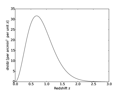
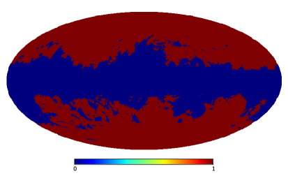
Figure 1: Selection function used in our numerical tests of different radial weightings. The left panel shows radial part (similar to the one expected from the Euclid survey), while the right panel shows the angular part, that removes regions of high stellar density and extinction, in Galactic coordinates. The angular mask was based in the one used in [44, 9].

Fig. 2 shows that there is a significant gain in the SNR for all modes and redshifts when the angular KL modes are built from the $C_{\ell}$ of the projected density that uses our radial weights. The reason is that this $C_{\ell}$ has a shape closer to the thin slices’ $C_{\ell}$s than the unweighted one. We point out that the $C_{\ell}$ overall amplitude does not alter the derived KL modes.

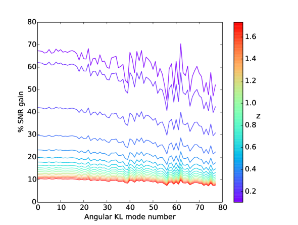
Figure 2: Fractional difference between the SNRs $S_{\mathrm{w}}$ and $S_{\mathrm{u}}$ ($S_{\mathrm{w}}/S_{\mathrm{u}}-1$) extracted from 16 thin redshift slices using angular KL modes built with weighted and unweighted projected $C_{\ell}$s, as a function of the first 78 KL modes (ordered by signal variance). The SNRs were computed with Eqs. 2.20 and 3.10 for each bin (colored according to their central redshift value) using the bin’s auto-$C_{\ell}$s.

It is worth pointing out that, in most cosmological models (as well as in the standard model), scales with the largest signal are intermediate ones. Consequently, these will be the scales probed by the KL modes constructed from a $C_{\ell}$ based on actual expected data. In case we want to build modes to probe the largest scales, one solution is to adopt a fiducial $C_{\ell}$ with boosted power on these scales. As mentioned above, this will not affect the orthogonality of the modes inside the survey’s mask and with respect to systematics’ maps, although it will turn the optimal radial weighting innocuous. Lastly, the RSD and lensing effects tend to increase the power on the largest scales [45], so the boosted fiducial $C_{\ell}$ is likely close to optimal.

The results from this section does not only serve as the angular part of 3D pKL modes, but also as a full KL method to analyze 2D, projected data. Moreover, our discussion of optimal weighting also applies to the quest of building a single set of angular KL modes to extract information for a set of tomographic slices of 3D cosmological fields.

3.2 Light-cone effects and new radial modes

Once the angular pKL modes $\Psi_{i}^{\mathrm{\theta}}(\mathbf{\hat{r}})$ are specified, we can write

$$\Psi_{[ij]}(\mathbf{r})=\mathcal{M}^{(i)}_{jn}\Phi_{n}^{\mathrm{z}}(r)\Psi_{(i)}^{\mathrm{\theta}}(\mathbf{\hat{r}})=\mathcal{M}^{\mathrm{\theta}}_{ip}\mathcal{M}^{(i)}_{jn}\Phi_{n}^{\mathrm{z}}(r)\Phi_{p}^{\mathrm{\theta}}(\mathbf{\hat{r}}),$$ (3.11)

remembering that we adopt the Einstein summation convention except for indices inside parentheses. In Eq. 3.11 we also chose to name the final pKL mode using a compound index made of two auxiliary indices, one for the angular part and the other for the radial part. What Eq. 3.11 says is that, for each angular mode $\Psi_{i}^{\mathrm{\theta}}(\mathbf{\hat{r}})$ held fixed, we will build a set of 3D modes $\Psi_{[ij]}(\mathbf{r})$ (where $i$ and $j$ select the angular and radial part, respectively) whose radial part is a linear combination of radial basis functions $\Phi_{n}^{\mathrm{z}}(r)$. Note that this linear combination is different for each angular mode, even if the radial index $j$ is the same, e.g.: $\mathcal{M}^{(1)}_{jn}\neq\mathcal{M}^{(2)}_{jn}$.

The choice for the radial basis functions $\Phi_{n}^{\mathrm{z}}(r)$ made in [30] was logarithmic waves [46]:

$$Z_{\omega}(r)\equiv\frac{1}{\sqrt{2\pi}}\frac{e^{-i\omega\ln(r)}}{r^{3/2}}.$$ (3.12)

This choice simplifies further calculations if light-cone effects can be ignored (i.e. if all galaxies in the survey are observed at the same Universe’s age) and if $\alpha(r)$, defined below, can be considered constant:

$$\alpha(r)\equiv\frac{\partial\ln[r^{2}\bar{n}_{\mathrm{g}}(r)]}{\partial\ln r}.$$ (3.13)

On the downside, $Z_{\omega}(r)$ are only orthogonal inside the interval $[0,\infty)$ and $\omega$, the number that characterizes the mode’s scale, is real and continuous. This last property is particularly unpleasant since it does not clear out which modes – and how many – are required to describe $\Psi^{\mathrm{z}}_{i}(r)$ up to a certain scale of interest. For this reason – and given that we take into consideration light-cone effects – we suggest the use of radial basis functions $\Phi_{n}^{\mathrm{z}}(r)$ that completely describes functions in a finite interval. Possible choices are discrete Fourier series, Legendre or Chebyshev polynomials or top-hat bins.

Legendre and Chebyshev polynomials have the advantage they are defined in a (non-periodic) finite interval (in contrast to Fourier series, which are periodical). Therefore, they may provide better descriptions for functions that would be discontinuous at periodic boundaries [e.g. $\bar{n}_{\mathrm{g}}(r)$], as they do not suffer from the Gibbs phenomenon. On the other hand, discrete Fourier series or top-hat functions might be easier to integrate (due to the use of fast Fourier transforms in the first and to the avoidance of oscillatory functions in the last case). Despite this choice, the final radial KL modes should be independent of the basis used (up to a certain scale).

To compute the radial $\mathcal{M}^{(i)}_{jn}$, we follow the usual procedure, described in Sec. 2.3, observing that it is not required to adopt the same choice for $w_{\mathrm{z}}(r)$ as in Sec. 3.1, now that $\Psi_{(i)}^{\mathrm{\theta}}(\mathbf{\hat{r}})$ is already built. Independently from the chosen radial basis, the first step is the orthogonalization with respect to the radial component of the systematics, $M^{\mathrm{z}}_{j}(r)$. As usual, we will use Eq. 2.15 with elements of $\mathsf{U}$ given by:

$$U^{\mathrm{z}}_{kj}=\int\frac{M^{\mathrm{z}}_{j}(r)}{w_{z}(r)}\Phi_{k}^{\mathrm{z}}(r)r^{2}\mathrm{d}r.$$ (3.14)

For separable $\bar{n}_{\mathrm{obs}}(\mathbf{r})$, the pre-whitening matrix $\mathsf{W}$ is obtained from the procedure described in Sec. 2.3, starting from:

$$N^{\prime}_{ij}=\int W_{\mathrm{z}}(r)\frac{\bar{n}^{\mathrm{z}}_{\mathrm{obs}}(r)}{w^{2}_{\mathrm{z}}(r)}\Phi_{i}^{\mathrm{z}}(r)\Phi_{j}^{\mathrm{z}*}(r)r^{2}\mathrm{d}r.$$ (3.15)

In this case, both $\mathsf{\Pi}$ and $\mathsf{W}$ are the same for every angular mode $\Psi_{i}^{\mathrm{\theta}}(\mathbf{\hat{r}})$, since $\mathsf{U}$ and $\mathsf{N^{\prime}}$ are separable.

Since the signal covariance matrix is non-separable, each angular mode will require its own $\mathsf{K}$ matrix. To compute them, we assume that the preparation of optimal angular pKL modes (Sec. 3.1) already made the covariance signal matrix for basis modes $\Phi_{n}^{\mathrm{z}}(r)\Psi_{i}^{\mathrm{\theta}}(\mathbf{\hat{r}})$ sufficiently close to zero for components whose angular parts are different [e.g. $\Phi_{n}^{\mathrm{z}}(r)\Psi_{1}^{\mathrm{\theta}}(\mathbf{\hat{r}})$ and $\Phi_{m}^{\mathrm{z}}(r)\Psi_{2}^{\mathrm{\theta}}(\mathbf{\hat{r}})$ for any $m,n$]. Therefore, we only need to diagonalize the matrix $\mathsf{W^{\dagger}\Pi S^{\prime}\Pi^{\dagger}W}$ for the same $\Psi_{i}^{\mathrm{\theta}}(\mathbf{\hat{r}})$. We start by computing $\mathsf{S^{\prime}}$.

We will begin by relating the galaxy density contrast $\delta_{\mathrm{g}}(\mathbf{r})$ directly accessible by observations – i.e. in redshift space and on the light-cone – to the matter density contrast in configuration space and at a fixed time, $\delta_{0}(\mathbf{r})$. Assuming a linear galaxy bias $b(r)$ (that depends on $r$ both due to luminosity bias [20] and due to galaxy evolution) and linear perturbation theory, this relation can be written as $\delta_{\mathrm{g}}(\mathbf{r})=\hat{S}\delta_{0}(\mathbf{r})$, where the RSD operator $\hat{S}$ is given by [47]:

$$\hat{S}=b(r)D(r)+\left[\gamma(r)\frac{\partial}{\partial r}+D(r)f(r)\frac{\partial^{2}}{\partial r^{2}}\right]\nabla^{-2}.$$ (3.16)

In the equation above, $D(r)$ is the matter growth function (described in terms of $r$ since the observations are made on the light-cone), $f(r)$ is its logarithmic derivative $f\equiv\mathrm{d}\ln D/\mathrm{d}\ln a$ in terms of the scale factor $a$, $\nabla^{-2}$ is the inverse of the Laplacian operator [easier to implement when $\delta_{0}(\mathbf{r})$ is described in Fourier space], and $\gamma(r)$ is:

$$\gamma(r)\equiv\frac{2D(r)f(r)}{r}+\frac{1}{\bar{n}^{\mathrm{z}}_{\mathrm{g}}(r)}\frac{\partial[D(r)f(r)\bar{n}^{\mathrm{z}}_{\mathrm{g}}(r)]}{\partial r}.$$ (3.17)

The second step is to express $\delta_{0}(\mathbf{r})$ by its Fourier transform $\tilde{\delta}_{0}(\mathbf{k})$, such that:

$$\nabla^{-2}\delta_{0}(\mathbf{r})=\frac{1}{(2\pi)^{3}}\int\frac{-\tilde{\delta}_{0}(\mathbf{k})}{k^{2}}e^{i\mathbf{k}\cdot\mathbf{r}}\mathrm{d^{3}}k;$$ (3.18)

and the third step is to expand $e^{i\mathbf{k}\cdot\mathbf{r}}$ in spherical waves [i.e. spherical Bessel functions $j_{\ell}(x)$ and spherical harmonics]:

$$e^{i\mathbf{k}\cdot\mathbf{r}}=4\pi\sum_{\ell=0}^{\infty}\sum_{m=-\ell}^{\ell}i^{\ell}j_{\ell}(kr)Y^{*}_{\ell m}(\mathbf{\hat{k}})Y_{\ell m}(\mathbf{\hat{r}}).$$ (3.19)

With Eqs. 3.16, 3.18 and 3.19, we can compute $\delta_{\mathrm{g}}(\mathbf{r})=\hat{S}\delta_{0}(\mathbf{r})$:

$$\delta_{\mathrm{g}}(\mathbf{r})=\frac{1}{2\pi^{2}}\sum_{\ell,m}i^{\ell}\int\tilde{\delta}_{0}(\mathbf{k})G_{\ell}(k,r)Y^{*}_{\ell m}(\mathbf{\hat{k}})Y_{\ell m}(\mathbf{\hat{r}})\mathrm{d^{3}}k,$$ (3.20)

$$G_{\ell}(k,r)\equiv b(r)D(r)j_{\ell}(kr)-\gamma(r)\frac{j^{\prime}_{\ell}(kr)}{k}-D(r)f(r)j^{\prime\prime}_{\ell}(kr),$$ (3.21)

where $j^{\prime}_{\ell}(x)$ and $j^{\prime\prime}_{\ell}(x)$ are $j_{\ell}(x)$’s first and second derivatives.

Let us call $s_{[ij]}$ (for ‘signal’) the $x_{[ij]}$ term proportional to $\delta_{\mathrm{g}}(\mathbf{r})$:

$$s_{[ij]}\equiv\int W(\mathbf{r})\frac{\bar{n}_{\mathrm{g}}(\mathbf{r})}{w(\mathbf{r})}\delta_{\mathrm{g}}(\mathbf{r})\Psi_{[ij]}(\mathbf{r})\mathrm{d^{3}}r.$$ (3.22)

By inserting Eqs. 3.11 and 3.20 into Eq. 3.22 and inverting the order of the integrals on $\mathbf{r}$ and $\mathbf{k}$, we get:

$$s_{[ij]}=\frac{\mathcal{M}^{(i)}_{jn}}{2\pi^{2}}\sum_{\ell,m}i^{\ell}\int\tilde{\delta}_{0}(\mathbf{k})\tilde{G}_{\ell m}^{in}(k)Y^{*}_{\ell m}(\mathbf{\hat{k}})\mathrm{d^{3}}k,$$ (3.23)

$$\tilde{G}_{\ell m}^{in}(k)\equiv\mathcal{M}^{\theta}_{ip}J_{[\ell_{p}m_{p}][(\ell m)]}\left[\frac{W_{\mathrm{\theta}}\bar{n}^{\mathrm{\theta}}_{\mathrm{g}}}{w_{\mathrm{\theta}}}\right]\int W_{\mathrm{z}}(r)\frac{\bar{n}_{\mathrm{g}}^{\mathrm{z}}(r)}{w_{\mathrm{z}}(r)}\Phi^{\mathrm{z}}_{n}(r)G_{\ell}(k,r)r^{2}\mathrm{d}r.$$ (3.24)

Remembering that the matter power spectrum at a fixed time $P_{0}(k)$ is defined by:

$$\langle\tilde{\delta}_{0}(\mathbf{k})\tilde{\delta}^{*}_{0}(\mathbf{k^{\prime}})\rangle=(2\pi)^{3}P_{0}(k)\delta_{\mathrm{D}}^{3}(\mathbf{k}-\mathbf{k^{\prime}}),$$ (3.25)

we can compute the signal covariance matrix $S_{[ij][np]}$ of the 3D pKL coefficients:

$$S_{[ij][np]}=\langle s_{[ij]}s^{*}_{[np]}\rangle=\mathcal{M}^{(i)}_{jq}~{}\frac{2}{\pi}\int P_{0}(k)\sum_{\ell,m}\tilde{G}_{\ell m}^{iq}(k)\tilde{G}_{\ell m}^{nr*}(k)k^{2}\mathrm{d}k~{}\mathcal{M}^{(n)\dagger}_{rp}.$$ (3.26)

In the above equation, the term on the right is of the kind $\mathcal{M}\mathsf{S^{\prime}}\mathcal{M^{\dagger}}$, where $\mathcal{M}$ is the matrix of coefficients that describes radial pKL modes in terms of the radial basis functions, given a certain angular pKL mode (set by the indices $i$ and $n$). If we want to solve Eq. 3.26 for $\mathcal{M}^{(i)}_{jq}$, the problem is overdetermined, since this same set of coefficients must solve for all $n$ in $\mathcal{M}^{(n)\dagger}_{rp}$ (when $i\neq n$ we expect $S_{[ij][np]}=0$ since these are off-diagonal terms). However, we assume that the diagonalization of the angular modes’ signal covariance matrix already made these terms sufficiently close to zero, so we can find the radial coefficients $\mathcal{M}^{(i)}_{jq}$ by setting $n=i$ in Eq. 3.26 and following the standard procedure (third item of Sec. 2.3).

Fig. 3 shows examples of radial KL modes, computed for the largest angular mode $\Psi_{0}^{\mathrm{\theta}}(\mathbf{\hat{r}})$. To simplify the calculations, we assumed $\Psi_{0}^{\mathrm{\theta}}(\mathbf{\hat{r}})=1$. To select large-scale modes, we adopted a power-law $P_{0}(k)$ so the signal is largest on the largest scales. The radial KL modes form an orthonormal basis in the redshift interval probed by the survey ($0<z<2$).

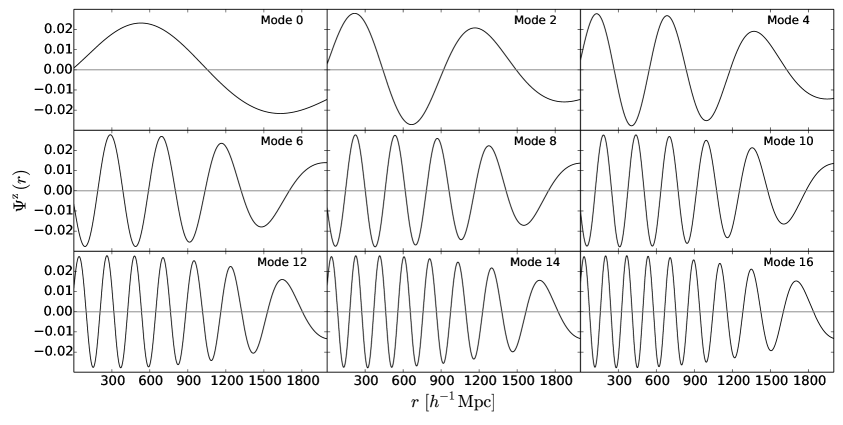
Figure 3: A few radial KL modes $\Psi_{i}^{\mathrm{z}}(r)$ computed for $\Psi_{0}^{\mathrm{\theta}}(\mathbf{\hat{r}})=1$. We adopted the radial weights $w_{\mathrm{z}}(r)=r\sqrt{\bar{n}^{\mathrm{z}}_{\mathrm{obs}}(r)}$, the redshift distribution shown in Fig. 1, 2000 top-hat basis functions covering the redshift range $0<z<2$, $P_{0}(k)=4000(k/0.1h\mathrm{Mpc^{-1}})^{-2.5}$ and remaining $\Lambda$CDM cosmological parameters given by Planck [48].

4 Building pKL modes for non-separable selection functions

Despite the efforts made by imaging and spectroscopic projects to cover the sky in a homogeneous way, it is very difficult to accomplish such task for the whole sky. For instance, on top of unanticipated calibration and technical problems and changes in pipelines that affected different regions of the sky, the SDSS data presented small differences between the north and south Galactic hemispheres [49]. Moreover, different instruments (such as those of the Euclid’s ground segment) also tend to result in slightly different galaxy selection functions and contamination rates. Given these challenges, we extended the pKL method for survey conditions that are non-separable into radial and angular parts; as a bonus, this extension allows the combined analysis of multiple surveys.

Our approach to deal with non-separable conditions is to assume they can be defined on angular sub-domains (i.e. they are piece-wise functions) and that in each sub-domain the separation between radial and angular parts is valid. This approach is adequate for the SDSS and WISE$\times$SuperCOSMOS [50] datasets, and should be valid for Euclid and LSST and also for combining data from different surveys. A concrete example is the analysis of SDSS Data Release 9 (DR9) galaxy distribution (see the left panel of Fig. 4), where we could describe the galaxy selection function in three sub-domains: the South Galactic Cap (SGC), and the regions in the North Galactic Cap (NGC) containing CMASS only and CMASS & LOWZ galaxies. In each of these sub-domains, the selection function can be considered separable. Since the window function $W(\mathbf{r})$ multiplies all terms in Eq. 2.1, it can be used as a “switch” for each one of the different separable selection functions defined over each sub-domain $h$: $W(\mathbf{r})=\sum_{h}W_{h}(\mathbf{r})$, where the non-zero regions of $W_{h}(\mathbf{r})$ do not overlap. Another real example is the WISE$\times$SuperCOSMOS catalog, built from observations made with different telescopes that lead to differences between the two equatorial hemispheres [50, 24]. These hemispheres can be described as sub-domains of separable selection functions (see the right panel of Fig. 4).

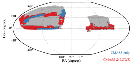
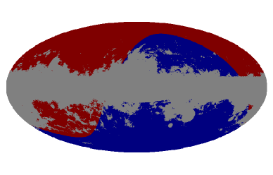
Figure 4: Left panel: map of the SDSS footprint in equatorial coordinates. The final BOSS footprint, with disjoint North (on the left) and South (on the right) Galactic Caps that present slightly different radial selection functions, is shown in gray. The colored dots represent the DR9 footprint: regions only containing observations of galaxies from the CMASS sample are presented in blue, while regions that also contain observations of galaxies from the LOWZ sample are presented in red. These two samples have very different radial selection functions. Figure from [41]. Right panel: mask of the WISE$\times$SuperCOSMOS catalog, in galactic coordinates, with the masked regions in gray. The red region is the northern equatorial hemisphere, observed with the POSS-II telescope, while the blue region is the southern equatorial hemisphere, observed with the UKST telescope [50].

For simplicity, we treat the case where there are two sub-domains with different $\bar{n}_{\mathrm{obs}}(\mathbf{r})$, indicated by the indices N and S (as in ‘North’ and ‘South’); however, the treatment of an arbitrary number of sub-domains is exactly the same and the generalization straightforward. In mathematical terms, this is given by:

$$\begin{split}n_{\mathrm{obs}}(\mathbf{r})=&W_{\mathrm{\theta}}^{\mathrm{N}}(\mathbf{\hat{r}})W_{\mathrm{z}}^{\mathrm{N}}(r)\{\bar{n}_{\mathrm{g}}^{\mathrm{\theta}}(\mathbf{\hat{r}})\bar{n}_{\mathrm{g}}^{\mathrm{z,N}}(r)[1+\delta_{\mathrm{g}}^{\mathrm{N}}(\mathbf{r})]+\epsilon(\mathbf{r})+s_{\mathrm{\theta}}^{\mathrm{N}}(\mathbf{\hat{r}})s_{\mathrm{z}}^{\mathrm{N}}(r)\}+\\ &W_{\mathrm{\theta}}^{\mathrm{S}}(\mathbf{\hat{r}})W_{\mathrm{z}}^{\mathrm{S}}(r)\{\bar{n}_{\mathrm{g}}^{\mathrm{\theta}}(\mathbf{\hat{r}})\bar{n}_{\mathrm{g}}^{\mathrm{z,S}}(r)[1+\delta_{\mathrm{g}}^{\mathrm{S}}(\mathbf{r})]+\epsilon(\mathbf{r})+s_{\mathrm{\theta}}^{\mathrm{S}}(\mathbf{\hat{r}})s_{\mathrm{z}}^{\mathrm{S}}(r)\}.\end{split}$$ (4.1)

In the equation above, we did not assign different angular parts $\bar{n}_{\mathrm{\theta}}(\mathbf{\hat{r}})$ to each sub-domain because the different $\mathbf{\hat{r}}$ already takes care of that [the same will happen to angular weights $w_{\mathrm{\theta}}(\mathbf{\hat{r}})$]. It is also worth remembering that the window function for one sub-domain is zero over the other sub-domains, and thus $W_{\mathrm{\theta}}^{\mathrm{N}}(\mathbf{\hat{r}})W_{\mathrm{\theta}}^{\mathrm{S}}(\mathbf{\hat{r}})=0$ for all $\mathbf{\hat{r}}$. We also considered the possibility that galaxy bias might be different in each sub-domain (e.g. due to different selection criteria). Luckily, the galaxy bias is always multiplied, in the equations, by the angular window function, such that in each sub-domain the bias can be described as dependent only on $r$.

4.1 Computing the angular pKL modes

We proceed through the same method described in Secs. 2.3 and 3, by computing the optimal angular modes. The first step is to determine the $\mathsf{\Pi}$ matrix. Since the systematics $M_{j}(\mathbf{r})$ describe $\langle n_{\mathrm{obs}}(\mathbf{r})\rangle$, they will also be described as piece-wise functions, e.g.: $M_{j}(\mathbf{r})=M_{j}^{\mathrm{N}}(\mathbf{r})+M_{j}^{\mathrm{S}}(\mathbf{r})$. From the definition of $M_{j}(\mathbf{r})$, we see this corresponds to simply increasing the number of systematic templates while the process of computing $\mathsf{\Pi}$ remains the same.

We continue by computing the angular modes’ pre-whitening matrix from $\mathsf{N^{\prime}}$. Since the Poisson noise $\epsilon(\mathbf{r})$ does not correlate at non-zero distances and $W_{\mathrm{\theta}}^{\mathrm{N}}(\mathbf{\hat{r}})$ and $W_{\mathrm{\theta}}^{\mathrm{S}}(\mathbf{\hat{r}})$ do not overlap, the basis modes’ noise covariance matrix $\mathsf{N^{\prime}}$ is simply the sum of the contributions coming from different sub-domains, each one computable by Eq. 3.2. Therefore, $\mathsf{N^{\prime}}$ becomes non-separable. In case $W_{\mathrm{z}}^{\mathrm{N}}(r)=W_{\mathrm{z}}^{\mathrm{S}}(r)$, this complication can be averted if and we adopt the radial weights $w_{\mathrm{z},h}(r)=r\sqrt{\bar{n}_{\mathrm{obs}}^{\mathrm{z,h}}(r)}$ ($h=\mathrm{N,S}$), thus making the radial part of $\mathsf{N^{\prime}}$ the same for every sub-domain and allowing us to factor it out. These weights happen to be the same as those that optimize the angular pKL modes (see Sec. 3.1). In any case, the noise covariance matrix of the angular basis functions is computed from Eq. 3.2 by fixing $\Phi_{i}^{\mathrm{z}}(r)=1$. Explicitly, we have:

$$N^{\prime}_{ij}=\int\left[I_{\mathrm{N}}W_{\mathrm{\theta}}^{\mathrm{N}}(\mathbf{\hat{r}})\frac{\bar{n}_{\mathrm{obs}}^{\mathrm{\theta}}(\mathbf{\hat{r}})}{w_{\mathrm{\theta}}^{2}(\mathbf{\hat{r}})}+I_{\mathrm{S}}W_{\mathrm{\theta}}^{\mathrm{S}}(\mathbf{\hat{r}})\frac{\bar{n}_{\mathrm{obs}}^{\mathrm{\theta}}(\mathbf{\hat{r}})}{w_{\mathrm{\theta}}^{2}(\mathbf{\hat{r}})}\right]\Phi_{i}^{\mathrm{\theta}}(\mathbf{\hat{r}})\Phi_{j}^{\mathrm{\theta}*}(\mathbf{\hat{r}})\mathrm{d^{2}}\hat{r},$$ (4.2)

$$I_{h}\equiv\int W_{\mathrm{z}}^{\mathrm{h}}(r)\frac{\bar{n}^{\mathrm{z,h}}_{\mathrm{obs}}(r)}{w_{\mathrm{z},h}^{2}(r)}r^{2}\mathrm{d}r.$$ (4.3)

If we use $\Phi_{i}^{\mathrm{\theta}}(\mathbf{\hat{r}})=Y^{*}_{\ell_{i}m_{i}}(\mathbf{\hat{r}})$, then:

$$\begin{split}N^{\prime}_{ij}=&J_{\ell_{i}m_{i}\ell_{j}m_{j}}\left[I_{\mathrm{N}}W_{\mathrm{\theta}}^{\mathrm{N}}\frac{\bar{n}_{\mathrm{obs}}^{\mathrm{\theta}}}{w_{\mathrm{\theta}}^{2}}+I_{\mathrm{S}}W_{\mathrm{\theta}}^{\mathrm{S}}\frac{\bar{n}_{\mathrm{obs}}^{\mathrm{\theta}}}{w_{\mathrm{\theta}}^{2}}\right]\\ =&I_{\mathrm{N}}J_{\ell_{i}m_{i}\ell_{j}m_{j}}\left[W_{\mathrm{\theta}}^{\mathrm{N}}\frac{\bar{n}_{\mathrm{obs}}^{\mathrm{\theta}}}{w_{\mathrm{\theta}}^{2}}\right]+I_{\mathrm{S}}J_{\ell_{i}m_{i}\ell_{j}m_{j}}\left[W_{\mathrm{\theta}}^{\mathrm{S}}\frac{\bar{n}_{\mathrm{obs}}^{\mathrm{\theta}}}{w_{\mathrm{\theta}}^{2}}\right].\end{split}$$ (4.4)

To derive the signal covariance matrix $\mathsf{S^{\prime}}$, we need to integrate the (weighted) observed density (Eq. 4.1) along the line of sight to work with the projected density contrast $\sigma_{\mathrm{g}}(\mathbf{\hat{r}})$. In this process, different selection functions will lead to different projected densities, so: $W_{\mathrm{\theta}}(\mathbf{\hat{r}})\sigma_{\mathrm{g}}(\mathbf{\hat{r}})=W_{\mathrm{\theta}}^{\mathrm{N}}(\mathbf{\hat{r}})\sigma_{\mathrm{g}}^{\mathrm{N}}(\mathbf{\hat{r}})+W_{\mathrm{\theta}}^{\mathrm{S}}(\mathbf{\hat{r}})\sigma_{\mathrm{g}}^{\mathrm{S}}(\mathbf{\hat{r}})$, where $\sigma_{\mathrm{g}}^{\mathrm{h}}(\mathbf{\hat{r}})$ is computed from Eq. 3.9 but with all functions specified for the sub-domain $h$. From Eq. 3.8, we see that $\mathsf{S^{\prime}}$ will be, like $\mathsf{N^{\prime}}$, a sum of contributions from different sub-domains; however, unlike $\mathsf{N^{\prime}}$, the signal from different sub-domains are correlated. Thus, we have:

$$S^{\prime}_{ij}={S^{\prime}}^{\mathrm{NN}}_{ij}+{S^{\prime}}^{\mathrm{NS}}_{ij}+{S^{\prime}}^{\mathrm{SN}}_{ij}+{S^{\prime}}^{\mathrm{SS}}_{ij},$$ (4.5)

where (in a similar way as in Eq. 3.10):

$${S^{\prime}}^{hk}_{ij}\equiv J_{[\ell_{i}m_{i}][\ell m]}\left[\frac{W_{\mathrm{\theta}}^{\mathrm{h}}\bar{n}^{\mathrm{\theta}}_{\mathrm{g}}}{w_{\mathrm{\theta}}}\right]C_{[\ell m][\ell^{\prime}m^{\prime}]}^{hk}J^{\dagger}_{[\ell^{\prime}m^{\prime}][\ell_{j}m_{j}]}\left[\frac{W_{\mathrm{\theta}}^{\mathrm{k}}\bar{n}^{\mathrm{\theta}}_{\mathrm{g}}}{w_{\mathrm{\theta}}}\right].$$ (4.6)

In the equation above, $C_{[\ell m][\ell^{\prime}m^{\prime}]}^{hk}=C^{hk}_{(\ell)}\delta^{\mathrm{K}}_{\ell\ell^{\prime}}\delta^{\mathrm{K}}_{mm^{\prime}}$ is the cross angular power spectrum (full-sky) of the projected densities $\sigma_{\mathrm{g}}^{h}(\mathbf{\hat{r}})$ and $\sigma_{\mathrm{g}}^{k}(\mathbf{\hat{r}})$.

Eq. 4.5 shows an interesting feature of the data: in principle, there is information in the cross-correlation between the two disjoint sectors (i.e. the total signal variance is not just the sum of the variances in each sector because the data has large scale correlations). To estimate the relevance of these cross terms, we considered the case of a hypothetical survey with the two sectors shown in the right panel of Fig. 4, in red and in blue. To make things simple, we assumed the only potential difference between the two sectors is the mean projected density.

We employed a monotonically decreasing $C_{\ell}$ to enforce the building of angular KL modes that probe the largest scales. The first four derived angular KL modes are shown in Fig. 5. Specially from the first three modes, it is easy to see that they are all orthogonal to the mean density in each hemisphere, separately. That is, uncertainties on the mean density in each hemisphere (and thus on their difference) do not affect the measured mode amplitude. Secondly, we note that none of the modes probe each hemisphere individually; they all account for density fluctuations in both hemispheres at the same time. This evidences that there is information in the cross-correlation between both hemispheres.

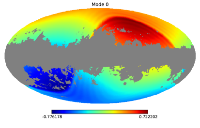
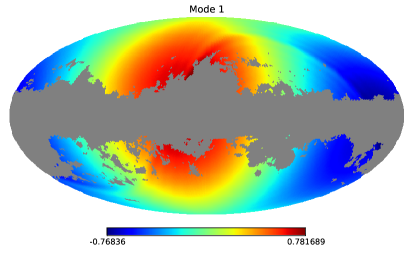
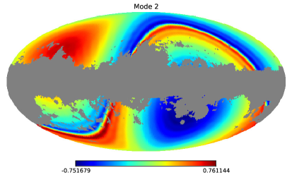
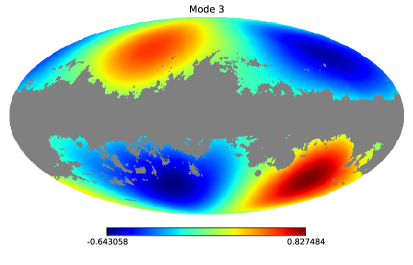
Figure 5: The first four angular KL modes to probe the largest scales, assuming a survey comprised of two disjoint regions depicted in the right panel of Fig. 4. The oscillations near the border between the northern and southern hemispheres, easily seen in modes 0 and 2, are artifacts known as Gibbs phenomenon.

We also can verify that the KL modes extract information across sectors by computing their fractional contribution to the diagonal of the total signal matrix, that is: $(\mathsf{S}^{\mathrm{NS}}+\mathsf{S}^{\mathrm{SN}})_{(ii)}/(\mathsf{S}^{\mathrm{NN}}+\mathsf{S}^{\mathrm{NS}}+\mathsf{S}^{\mathrm{SN}}+\mathsf{S}^{\mathrm{SS}})_{(ii)}$, where $\mathsf{S}^{\mathrm{hk}}=\mathcal{M}\mathsf{S^{\prime}}^{\mathrm{hk}}\mathcal{M}^{\dagger}$ and _(ii) denotes the $i$th element of the diagonal. Fig. 6 shows these quantities for the case discussed here (two sectors as in the right panel of Fig. 4) and for the same case but with a 13^∘-wide buffer zone between the northern and southern hemispheres (i.e. we masked out the frontier between the two sectors). We see that the cross-terms contribute to the signal, specially on the largest scales where it reaches up to $\sim$15% of the total. The fact that the buffer zone significantly reduces the cross-term contribution tells us that the information across sectors comes from data correlations near their border. This makes sense as density correlations rapidly decrease with distance but still do not care if they cross human-made boundaries.

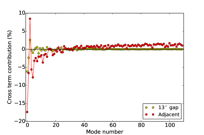
Figure 6: Fraction of the expected variance of the coefficients describing the weighted projected density in terms of angular KL modes that comes from cross-correlations between two disjoint sky sectors, as a function of mode number (largest scales first). The red dots represent the results obtained for the two hemispheres shown in the right panel of Fig. 4, while the ochre dots represent the results for the same hemispheres but with a $13^{\circ}$ wide buffer zone (masked region) between the two hemispheres. See the text for the exact expression generating these values.

4.2 Computing the radial pKL modes

Just like for the angular part described in the previous section, the separation of the selection function in sub-domains multiplies the amount of systematic templates the radial part has to deal with. That is, the matrix $\mathsf{\Pi}$ needs to project out from $\Psi^{\mathrm{z}}_{i}(r)$ the radial part $M_{j}^{\mathrm{z}}(r)$ of all templates (from all sub-domains).

When dealing with piece-wise separable selection functions like we do in this section, the process of pre-whitening the noise covariance matrix for the 3D pKL modes (Eq. 2.16) can be slightly more complicated if the radial window functions for each sub-domain $h$, $W_{\mathrm{z}}^{h}(r)$, are different: in this case we cannot use radial weights to factor out the radial part (see Sec. 4.1). Once the angular pKL modes $\Psi_{i}^{\mathrm{\theta}}(\mathbf{\hat{r}})$ are defined from Eq. 4.2, the matrix $\mathsf{N^{\prime}}$ for the 3D pKL modes will be a sum of contributions from each sub-domain:

$$\begin{split}N^{\prime}_{[ni][mj]}=&\int W_{\mathrm{z}}^{\mathrm{N}}(r)\frac{\bar{n}^{\mathrm{z,N}}_{\mathrm{obs}}(r)}{w^{2}_{\mathrm{z,N}}(r)}\Phi_{n}^{\mathrm{z}}(r)\Phi_{m}^{\mathrm{z}*}(r)r^{2}\mathrm{d}r\int W_{\mathrm{\theta}}^{\mathrm{N}}(\mathbf{\hat{r}})\frac{\bar{n}^{\mathrm{\theta}}_{\mathrm{obs}}(\mathbf{\hat{r}})}{w^{2}_{\mathrm{\theta}}(\mathbf{\hat{r}})}\Psi_{i}^{\mathrm{\theta}}(\mathbf{\hat{r}})\Psi_{j}^{\mathrm{\theta}*}(\mathbf{\hat{r}})\mathrm{d^{2}}\hat{r}~{}+\\ &\int W_{\mathrm{z}}^{\mathrm{S}}(r)\frac{\bar{n}^{\mathrm{z,S}}_{\mathrm{obs}}(r)}{w^{2}_{\mathrm{z,S}}(r)}\Phi_{n}^{\mathrm{z}}(r)\Phi_{m}^{\mathrm{z}*}(r)r^{2}\mathrm{d}r\int W_{\mathrm{\theta}}^{\mathrm{S}}(\mathbf{\hat{r}})\frac{\bar{n}^{\mathrm{\theta}}_{\mathrm{obs}}(\mathbf{\hat{r}})}{w^{2}_{\mathrm{\theta}}(\mathbf{\hat{r}})}\Psi_{i}^{\mathrm{\theta}}(\mathbf{\hat{r}})\Psi_{j}^{\mathrm{\theta}*}(\mathbf{\hat{r}})\mathrm{d^{2}}\hat{r}.\end{split}$$ (4.7)

The problem is that, as Eq. 4.2 shows, $\Psi_{i}^{\mathrm{\theta}}(\mathbf{\hat{r}})$ are built to yield a unit noise covariance matrix only when applied to the combination of sub-domains N and S, weighted by $I_{\mathrm{N}}$ and $I_{\mathrm{S}}$ (Eq. 4.3), whereas Eq. 4.7 shows that a combination of radial basis modes $\Phi_{n}^{\mathrm{z}}(r)$ would only result in an unit 3D noise covariance matrix if $\Psi_{i}^{\mathrm{\theta}}(\mathbf{\hat{r}})$ led to a unit noise covariance matrix in each sub-domain separately. Consequently, we assume $W_{\mathrm{z}}^{\mathrm{N}}(r)=W_{\mathrm{z}}^{\mathrm{S}}(r)=W_{\mathrm{z}}(r)$ and adopt the weights:

$$w_{\mathrm{z,h}}(r)=r\sqrt{\frac{\bar{n}^{\mathrm{z},h}_{\mathrm{obs}}(r)}{I_{h}}},$$ (4.8)

allowing us to factor out the radial part:

$$\begin{split}N^{\prime}_{[ni][mj]}=&\int W_{\mathrm{z}}(r)\Phi_{n}^{\mathrm{z}}(r)\Phi_{m}^{\mathrm{z}*}(r)\mathrm{d}r\int\left[I_{\mathrm{N}}W_{\mathrm{\theta}}^{\mathrm{N}}(\mathbf{\hat{r}})\frac{\bar{n}_{\mathrm{obs}}^{\mathrm{\theta}}(\mathbf{\hat{r}})}{w_{\mathrm{\theta}}^{2}(\mathbf{\hat{r}})}+I_{\mathrm{S}}W_{\mathrm{\theta}}^{\mathrm{S}}(\mathbf{\hat{r}})\frac{\bar{n}_{\mathrm{obs}}^{\mathrm{\theta}}(\mathbf{\hat{r}})}{w_{\mathrm{\theta}}^{2}(\mathbf{\hat{r}})}\right]\Psi_{i}(\mathbf{\hat{r}})\Psi_{j}^{*}(\mathbf{\hat{r}})\mathrm{d^{2}}\hat{r}\\ =&\int W_{\mathrm{z}}(r)\Phi_{n}^{\mathrm{z}}(r)\Phi_{m}^{\mathrm{z}*}(r)\mathrm{d}r~{}\delta^{\mathrm{K}}_{ij}.\end{split}$$ (4.9)

In other words, under these conditions we only need to find a pre-whitening matrix $\mathsf{W}$ that turns $\Pi_{kn}\int W_{\mathrm{z}}(r)\Phi_{n}^{\mathrm{z}}(r)\Phi_{m}^{\mathrm{z}*}(r)\mathrm{d}r~{}\Pi^{\dagger}_{mp}$ into the identity matrix.

Finally, we need to compute a matrix $\mathsf{S^{\prime}}$ for the radial modes, one for each angular part $\Psi_{i}^{\mathrm{\theta}}(\mathbf{\hat{r}})$ (as in Sec. 3.2). Just like for the angular modes in the previous section, we can write $\mathsf{S^{\prime}}$ as a sum of contributions from each sub-domain (and from their cross-correlations). Explicitly, we obtain:

$${S^{\prime}}_{[in][jp]}=\frac{2}{\pi}\int P_{0}(k)\sum_{h,h^{\prime}}\sum_{\ell,m}\tilde{G}_{\ell m}^{h,in}(k)\tilde{G}_{\ell m}^{h^{\prime},jp*}(k)k^{2}\mathrm{d}k,$$ (4.10)

$$\tilde{G}_{\ell m}^{h,in}(k)\equiv\mathcal{M}^{\theta}_{i[LM]}J_{[LM][(\ell m)]}\left[W_{\mathrm{\theta}}^{(h)}\frac{\bar{n}^{\mathrm{\theta}}_{\mathrm{g}}}{w_{\mathrm{\theta}}}\right]\int\Phi^{\mathrm{z}*}_{n}(r)\frac{\bar{n}_{\mathrm{g}}^{\mathrm{z}(h)}(r)}{w_{\mathrm{z}(h)}(r)}G^{(h)}_{\ell}(k,r)r^{2}\mathrm{d}r,$$ (4.11)

$$G^{h}_{\ell}(k,r)\equiv b_{h}(r)D(r)j_{\ell}(kr)-\gamma_{h}(r)\frac{j^{\prime}_{\ell}(kr)}{k}-D(r)f(r)j^{\prime\prime}_{\ell}(kr),$$ (4.12)

$$\gamma_{h}(r)\equiv\frac{2D(r)f(r)}{r}+\frac{1}{\bar{n}^{\mathrm{z}(h)}_{\mathrm{g}}(r)}\frac{\partial[D(r)f(r)\bar{n}^{\mathrm{z}(h)}_{\mathrm{g}}(r)]}{\partial r}.$$ (4.13)

In the equations above, the indices $i$ and $j$ identify the angular part of the pKL modes, while $n$ and $p$ identify the radial basis functions; $h$ and $h^{\prime}$ informs to which sub-domain each function belongs to; and $\ell$ and $m$ are the usual spherical harmonic multipoles indices. We also remind that we adopt the Einstein summation convention except for indices inside parentheses, that compound indices (representing a single dimension) are written inside square brackets and that the weights $w_{\mathrm{z},h}(r)$ are given by Eq. 4.8. Again, the matrix $\mathsf{K}$ is obtained for each angular mode $\Psi_{i}^{\mathrm{\theta}}(\mathbf{\hat{r}})$ following the third item in Sec. 2.3 and using Eq. 4.10 with $i=j$.

5 Using pKL to measure $P_{0}(k)$

The previous sections dealt with the issue of finding optimal (pKL) modes $\Psi_{i}(\mathbf{r})$ to measure the clustering of galaxies, given the survey’s characteristics and assuming a fiducial $P_{0}(k)$. Although defining $\Psi_{i}(\mathbf{r})$ can be a lengthy process, once this is done it is straightforward to use them to measure $P_{0}(k)$.

The first step is to compute the coefficients $x_{i}$ that describe the observed density in terms of the pKL modes (Eq. 2.3), using the radial weights given by Eq. 4.8. As Eq. 2.4 shows, these coefficients have mean value zero, a feature that is completely independent of cosmology and therefore remains no matter the true value of $P_{0}(k)$. The covariance can be described as $\langle x_{i}x_{j}^{*}\rangle=S_{ij}+\delta^{\mathrm{K}}_{ij}$, and this fact also does not depend on cosmology (the noise covariance matrix, which is the identity matrix, only depends on the characteristics of the survey). Thus, all cosmological information is encoded in the signal covariance matrix, and in a rather simple way:

$$S_{ij}=\int P_{0}(k)H_{ij}(k)\mathrm{d}k,$$ (5.1)

where $H_{ij}(k)$ is pre-computed once and for all according to the designed optimal modes:

$$H_{[ir][js]}(k)\equiv\frac{2}{\pi}\mathcal{M}^{(i)}_{rn}\sum_{h,h^{\prime}}\sum_{\ell,m}\tilde{G}^{h,in}_{\ell m}(k)\tilde{G}^{h^{\prime},jp*}_{\ell m}(k)k^{2}\mathcal{M}^{(j)\dagger}_{ps}.$$ (5.2)

Since $x_{i}$ follow a Gaussian distribution [32], their likelihood function is well determined:

$$\mathcal{L}=\frac{1}{(2\pi)^{N/2}\sqrt{\det(\mathsf{S}+\mathsf{I})}}\exp\left[-\frac{1}{2}\mathsf{x}^{\dagger}(\mathsf{S}+\mathsf{I})^{-1}\mathsf{x}\right],$$ (5.3)

and we can take advantage of pKL compression and smaller number of modes that probe the largest scales to analyze $\mathcal{L}$ and find $P_{0}(k)$.

As a last strategy to speed up computations, we can model $P_{0}(k)$ as a piece-wise function of constant band-powers $p_{q}$:

$$P_{0}(k)=\sum_{q}p_{q}B_{q}(k),$$ (5.4)

where $B_{q}(k)$ are rectangular functions. Under this approach, Eq. 5.1 can be written as a weighted sum of pre-computed matrices:

$$S_{ij}=\sum_{q}p_{q}\int B_{q}(k)H_{ij}(k)\mathrm{d}k.$$ (5.5)

To highlight the importance of taking into account light-cone effects when measuring density fluctuations on the largest scales, we computed the signal covariance matrix $\mathsf{S}$ for the pKL modes presented in Fig. 3 assuming different cosmologies and compared to the case where light-cone effects are ignored. Fig. 7 shows the fractional difference of pKL modes’ variances with respect to a fiducial cosmology for these alternative cosmologies or approach.

It is evident that neglecting light-cone effects produces changes in $\mathsf{S}$ that are of the same order as reasonable changes in large-scale cosmological parameters (such as the spectral index $n_{\mathrm{s}}$ and running $\alpha_{\mathrm{s}}$ of the primordial power spectrum). Similar results might be expected if one is interested in measuring scale-dependent biases like those in [39, 37]. On smaller scales (larger mode numbers), the outcome of leaving light-cone effects out is degenerate to a constant factor change in $P_{0}(k)$ (i.e. changing the amplitude $A_{\mathrm{s}}$), and therefore such effects may not have to be taken into account at these scales.

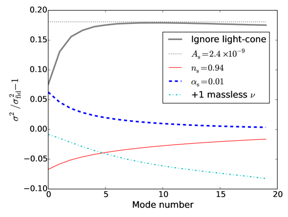
Figure 7: Fractional difference between the expected variance $\sigma^{2}$ of large-scale pKL modes (see Fig. 3) computed for variations over cosmological parameters and the variance $\sigma^{2}_{\mathrm{fid}}$ computed for a fiducial flat $\Lambda$CDM cosmology ($A_{\mathrm{s}}=2.2\times 10^{-9}$, $n_{\mathrm{s}}=0.96$, $\alpha_{\mathrm{s}}=0$, $\Omega_{\mathrm{b}}h^{2}=0.022$, $\Omega_{\mathrm{cdm}}h^{2}=0.12$ and 3 massless neutrinos). For each curve, we only varied one parameter. We also show as a thick gray curve the variance calculated when neglecting light-cone effects.

6 Discussion

In this paper we have presented in detail the pseudo Karhunen-Loève (pKL) method and its application to cosmology. This method includes the modes’ orthogonalization to systematics templates, a feature that makes the analysis less sensitive to contaminants and uncertainties on the mean density and/or observed dipole caused by our peculiar motion. This orthogonalization method has the advantage that it does not require the systematics contribution level to be determined; it only requires that systematics are properly modeled up to a constant factor. It is worth pointing out that this orthogonalization approach only mitigates additive systematics and not multiplicative ones. Strategies for dealing with multiplicative effects are given in [41, 23, 24].

During the orthogonalization process, the dimensionality of the space covered by the KL modes is reduced: all data is projected onto a sub-space that is orthogonal to the mean density and systematics templates. This hinders the subsequent step of pre-whitening the data because the covariance matrices become singular. We presented a solution for this in Eq. 2.19, where we identify redundant modes by their null variance. It is worth pointing out that the original dimensionality can be restored by including the systematics templates as “special modes”, since these are orthogonal to all other modes by construction. While the variance measured in these modes cannot be used to extract cosmological information, their amplitude provides an estimate of the level of contamination associated to a particular template.

As shown in Sec. 3, we simplify the application of the KL method to 3D data by first creating close to optimal angular modes that are later combined with radial ones to create full 3D modes. We proposed that these angular modes are obtained by applying the KL method to weighted instead of unweighted projected density of galaxies. The appropriate weights are those that make the noise level the same in every redshift slice (see Eq. 4.8). Sec. 3 can also be applied to tomographic analysis of galaxy surveys, in which case no simplifications to the KL method are made.

The SDSS and WISE$\times$SuperCOSMOS have indicated that achieving a constant radial selection function across the whole sky might be difficult, and this issue can affect future surveys such as the Euclid ground segment. Thus, we presented a generalization of previous implementations of the pKL method that can tackle this situation by segmenting the sky into patches with locally constant radial selection functions. This method can also be used to combine information from multiple surveys. Interestingly, in Sec. 4.1 we have also demonstrated that such combination leads to more information that the sum of its parts, given that galaxy densities are correlated over large distances (and across survey boundaries). This property is not unique to the pKL method and can be demonstrated for pseudo angular power spectra analysis (p$C_{\ell}$) [51] and the Landy-Szalay [13] configuration space estimator.

In the derivation and analysis of radial modes, we have taken into account the fact that our observations are made on the surface of our past light cone, and thus the farther we look in space, the farther we look in time. For deep enough surveys, the growth of structure and galaxy bias evolution along our line of sight must be taken into account. As shown in Fig. 7, these light-cone effects distort the observed clustering on the largest scales and could be confused (if not accounted for) with other physical effects like scale-dependent biases, different primordial spectral indices and their runnings. The combination of proper modeling of this evolution in the radial direction with the use of distinct sky sectors and their resulting synergy makes the method presented here a powerful tool to probe the largest scales in the Universe.

References

- [1] W. J. Percival, C. M. Baugh, J. Bland-Hawthorn, T. Bridges, R. Cannon, S. Cole et al., The 2dF Galaxy Redshift Survey: the power spectrum and the matter content of the Universe, MNRAS 327 (2001) 1297 [astro-ph/0105252].
- [2] D. J. Eisenstein, I. Zehavi, D. W. Hogg, R. Scoccimarro, M. R. Blanton, R. C. Nichol et al., Detection of the Baryon Acoustic Peak in the Large-Scale Correlation Function of SDSS Luminous Red Galaxies, ApJ 633 (2005) 560 [astro-ph/0501171].
- [3] C. Blake, S. Brough, M. Colless, C. Contreras, W. Couch, S. Croom et al., The WiggleZ Dark Energy Survey: the growth rate of cosmic structure since redshift z=0.9, MNRAS 415 (2011) 2876 [1104.2948].
- [4] A. J. Ross, W. J. Percival, A. Carnero, G.-b. Zhao, M. Manera, A. Raccanelli et al., The clustering of galaxies in the SDSS-III DR9 Baryon Oscillation Spectroscopic Survey: constraints on primordial non-Gaussianity, MNRAS 428 (2013) 1116 [1208.1491].
- [5] S. Riemer-Sørensen, C. Blake, D. Parkinson, T. M. Davis, S. Brough, M. Colless et al., WiggleZ Dark Energy Survey: Cosmological neutrino mass constraint from blue high-redshift galaxies, PRD 85 (2012) 081101 [1112.4940].
- [6] A. G. Sánchez, E. A. Kazin, F. Beutler, C.-H. Chuang, A. J. Cuesta, D. J. Eisenstein et al., The clustering of galaxies in the SDSS-III Baryon Oscillation Spectroscopic Survey: cosmological constraints from the full shape of the clustering wedges, MNRAS 433 (2013) 1202 [1303.4396].
- [7] P. Laurent, J.-M. Le Goff, E. Burtin, J.-C. Hamilton, D. W. Hogg, A. Myers et al., A 14 h-3 Gpc3 study of cosmic homogeneity using BOSS DR12 quasar sample, JCAP 11 (2016) 060 [1602.09010].
- [8] C. A. P. Bengaly, Jr., A. Bernui, J. S. Alcaniz, H. S. Xavier and C. P. Novaes, Is there evidence for anomalous dipole anisotropy in the large-scale structure?, MNRAS 464 (2017) 768 [1606.06751].
- [9] C. P. Novaes, A. Bernui, H. S. Xavier and G. A. Marques, Tomographic local 2D analyses of the WISExSuperCOSMOS all-sky galaxy catalogue, MNRAS 478 (2018) 3253 [1805.04078].
- [10] E. de Carvalho, A. Bernui, G. C. Carvalho, C. P. Novaes and H. S. Xavier, Angular Baryon Acoustic Oscillation measure at z=2.225 from the SDSS quasar survey, JCAP 4 (2018) 064 [1709.00113].
- [11] D. Jeong, Cosmology with high () redshift galaxy surveys, Ph.D. thesis, University of Texas at Austin (djeong@astro.as.utexas.edu), August, 2010.
- [12] B. Leistedt and J. D. McEwen, Exact Wavelets on the Ball, IEEE Transactions on Signal Processing 60 (2012) 6257 [1205.0792].
- [13] S. D. Landy and A. S. Szalay, Bias and variance of angular correlation functions, ApJ 412 (1993) 64.
- [14] H. A. Feldman, N. Kaiser and J. A. Peacock, Power-spectrum analysis of three-dimensional redshift surveys, ApJ 426 (1994) 23 [astro-ph/9304022].
- [15] M. Tegmark, A Method for Extracting Maximum Resolution Power Spectra from Galaxy Surveys, ApJ 455 (1995) 429 [astro-ph/9502012].
- [16] A. F. Heavens and A. N. Taylor, A spherical harmonic analysis of redshift space, MNRAS 275 (1995) 483 [astro-ph/9409027].
- [17] A. J. S. Hamilton, Linear Redshift Distortions: a Review, in The Evolving Universe (D. Hamilton, ed.), vol. 231 of Astrophysics and Space Science Library, p. 185, 1998, astro-ph/9708102, DOI.
- [18] K. Yamamoto, M. Nakamichi, A. Kamino, B. A. Bassett and H. Nishioka, A Measurement of the Quadrupole Power Spectrum in the Clustering of the 2dF QSO Survey, PASJ 58 (2006) 93 [astro-ph/0505115].
- [19] E. A. Kazin, A. G. Sánchez and M. R. Blanton, Improving measurements of and by analysing clustering anisotropies, MNRAS 419 (2012) 3223 [1105.2037].
- [20] W. J. Percival, L. Verde and J. A. Peacock, Fourier analysis of luminosity-dependent galaxy clustering, MNRAS 347 (2004) 645 [astro-ph/0306511].
- [21] D. J. Eisenstein, H.-J. Seo, E. Sirko and D. N. Spergel, Improving Cosmological Distance Measurements by Reconstruction of the Baryon Acoustic Peak, ApJ 664 (2007) 675 [astro-ph/0604362].
- [22] F. Simpson, A. F. Heavens and C. Heymans, Clipping the cosmos. II. Cosmological information from nonlinear scales, PRD 88 (2013) 083510 [1306.6349].
- [23] D. L. Shafer and D. Huterer, Multiplicative errors in the galaxy power spectrum: self-calibration of unknown photometric systematics for precision cosmology, MNRAS 447 (2015) 2961 [1410.0035].
- [24] H. S. Xavier, M. V. Costa-Duarte, A. Balaguera-Antolínez and M. Bilicki, All-sky angular power spectra from cleaned WISESuperCOSMOS galaxy number counts, arXiv e-prints (2018) [1812.08182].
- [25] F. Elsner, B. Leistedt and H. V. Peiris, Unbiased pseudo- power spectrum estimation with mode projection, MNRAS 465 (2017) 1847 [1609.03577].
- [26] M. Tegmark, A. N. Taylor and A. F. Heavens, Karhunen-Loève Eigenvalue Problems in Cosmology: How Should We Tackle Large Data Sets?, ApJ 480 (1997) 22 [astro-ph/9603021].
- [27] M. Tegmark, A. J. S. Hamilton, M. A. Strauss, M. S. Vogeley and A. S. Szalay, Measuring the Galaxy Power Spectrum with Future Redshift Surveys, ApJ 499 (1998) 555 [astro-ph/9708020].
- [28] M. S. Vogeley and A. S. Szalay, Eigenmode Analysis of Galaxy Redshift Surveys. I. Theory and Methods, ApJ 465 (1996) 34 [astro-ph/9601185].
- [29] M. Colless, G. Dalton, S. Maddox, W. Sutherland, P. Norberg, S. Cole et al., The 2dF Galaxy Redshift Survey: spectra and redshifts, MNRAS 328 (2001) 1039 [astro-ph/0106498].
- [30] M. Tegmark, A. J. S. Hamilton and Y. Xu, The power spectrum of galaxies in the 2dF 100k redshift survey, MNRAS 335 (2002) 887 [astro-ph/0111575].
- [31] D. G. York, J. Adelman, J. E. Anderson, Jr., S. F. Anderson, J. Annis, N. A. Bahcall et al., The Sloan Digital Sky Survey: Technical Summary, AJ 120 (2000) 1579 [astro-ph/0006396].
- [32] M. Tegmark, M. R. Blanton, M. A. Strauss, F. Hoyle, D. Schlegel, R. Scoccimarro et al., The Three-Dimensional Power Spectrum of Galaxies from the Sloan Digital Sky Survey, ApJ 606 (2004) 702 [astro-ph/0310725].
- [33] D. Lumb, L. Duvet, R. Laurijs, M. Te Plate, I. Escudero Sanz and G. Saavedra Criado, Euclid Mission: assessment study, in UV/Optical/IR Space Telescopes: Innovative Technologies and Concepts IV, vol. 7436 of Proc. SPIE, p. 743604, Aug., 2009, DOI.
- [34] LSST Science Collaboration, P. A. Abell, J. Allison, S. F. Anderson, J. R. Andrew, J. R. P. Angel et al., LSST Science Book, Version 2.0, arXiv e-prints (2009) arXiv:0912.0201 [0912.0201].
- [35] DESI Collaboration, A. Aghamousa, J. Aguilar, S. Ahlen, S. Alam, L. E. Allen et al., The DESI Experiment Part I: Science,Targeting, and Survey Design, arXiv e-prints (2016) [1611.00036].
- [36] N. Benitez, R. Dupke, M. Moles, L. Sodre, J. Cenarro, A. Marin-Franch et al., J-PAS: The Javalambre-Physics of the Accelerated Universe Astrophysical Survey, arXiv e-prints (2014) [1403.5237].
- [37] N. Dalal, O. Doré, D. Huterer and A. Shirokov, Imprints of primordial non-Gaussianities on large-scale structure: Scale-dependent bias and abundance of virialized objects, PRD 77 (2008) 123514 [0710.4560].
- [38] R. de Putter and O. Doré, Designing an inflation galaxy survey: How to measure (fNL)1 using scale-dependent galaxy bias, PRD 95 (2017) 123513 [1412.3854].
- [39] R. Durrer, A. Gabrielli, M. Joyce and F. Sylos Labini, Bias and the Power Spectrum beyond the Turnover, ApJ 585 (2003) L1 [astro-ph/0211653].
- [40] M. Takada, Can a galaxy redshift survey measure dark energy clustering?, PRD 74 (2006) 043505 [astro-ph/0606533].
- [41] A. J. Ross, W. J. Percival, A. G. Sánchez, L. Samushia, S. Ho, E. Kazin et al., The clustering of galaxies in the SDSS-III Baryon Oscillation Spectroscopic Survey: analysis of potential systematics, MNRAS 424 (2012) 564 [1203.6499].
- [42] B. Jain, D. Spergel, R. Bean, A. Connolly, I. Dell’antonio, J. Frieman et al., The Whole is Greater than the Sum of the Parts: Optimizing the Joint Science Return from LSST, Euclid and WFIRST, arXiv e-prints (2015) [1501.07897].
- [43] M. Bilicki, T. H. Jarrett, J. A. Peacock, M. E. Cluver and L. Steward, Two Micron All Sky Survey Photometric Redshift Catalog: A Comprehensive Three-dimensional Census of the Whole Sky, ApJS 210 (2014) 9 [1311.5246].
- [44] C. A. P. Bengaly, C. P. Novaes, H. S. Xavier, M. Bilicki, A. Bernui and J. S. Alcaniz, The dipole anisotropy of WISE SuperCOSMOS number counts, MNRAS 475 (2018) L106 [1707.08091].
- [45] A. Challinor and A. Lewis, Linear power spectrum of observed source number counts, PRD 84 (2011) 043516 [1105.5292].
- [46] A. J. S. Hamilton and M. Culhane, Spherical redshift distortions, MNRAS 278 (1996) 73 [astro-ph/9507021].
- [47] T. Matsubara, The Correlation Function in Redshift Space: General Formula with Wide-Angle Effects and Cosmological Distortions, ApJ 535 (2000) 1 [astro-ph/9908056].
- [48] Planck Collaboration, P. A. R. Ade, N. Aghanim, M. Arnaud, M. Ashdown, J. Aumont et al., Planck 2015 results. XIII. Cosmological parameters, A&A 594 (2016) A13 [1502.01589].
- [49] B. Reid, S. Ho, N. Padmanabhan, W. J. Percival, J. Tinker, R. Tojeiro et al., SDSS-III Baryon Oscillation Spectroscopic Survey Data Release 12: galaxy target selection and large-scale structure catalogues, MNRAS 455 (2016) 1553 [1509.06529].
- [50] M. Bilicki, J. A. Peacock, T. H. Jarrett, M. E. Cluver, N. Maddox, M. J. I. Brown et al., WISE SuperCOSMOS Photometric Redshift Catalog: 20 Million Galaxies over 3 Steradians, ApJS 225 (2016) 5 [1607.01182].
- [51] D. Alonso, J. Sanchez and A. Slosar, A unified pseudo- framework, arXiv e-prints (2018) [1809.09603].