The many avatars of Curzon-Ahlborn efficiency

Abstract

Efficiency at maximum power output of irreversible heat engines has attracted a lot of interest in recent years. We discuss the occurence of a particularly simple and elegant formula for this efficiency in various different models. The so-called Curzon-Ahlborn efficiency is given by the square-root formula: $1-\sqrt{T_{c}/T_{h}}$, where $T_{c}$ and $T_{h}$ are the cold and hot reservoir temperatures.

I Introduction

Industrial revolution fueled our efforts to understand the working of thermal machines to improve their performance. This gave rise to the science of thermodynamics which identifies the permissible limits—put by physical laws—on our energy conversion devices. Carnot’s insight on the maximum efficiency of a heat engine operating between two heat reservoirs at temperatures $T_{h}$ (hot) and $T_{c}$ (cold), yielded the universal expression:

$$\eta_{C}=1-\frac{T_{c}}{T_{h}},$$ (1)

which involves only the ratio of the temperatures, and is independent of the details of the working medium. However, Carnot bound is not realistic for actual heat engines and power plants. Naturally, real machines operate under irreversibilities caused by various factors, like finite rates of energy and matter flows, internal friction, heat leakage and so on, unlike the idealized quasi-static processes of textbook models. Further, real engines are required to produce a finite power output within a finite cycle time, whereas the power output of a Carnot engine vanishes due to infeasibly large cycle times. In fact, the observed efficiencies are usually much less than the Carnot limit. Thus the analysis of irreversible models with finite-rate processes seems a desirable goal to pursue.

In recent years, there has been a great interest in extending thermodynamic models to justify the observed performance of industrial power plants Curzon and Ahlborn (1975); Bejan (1997); Esposito et al. (2010). An interesting quantity is the efficiency at maximum power (EMP) of an irreversible model. An elegant expression is often derived in some models, given as

$$\eta_{CA}=1-\sqrt{\frac{T_{c}}{T_{h}}}.$$ (2)

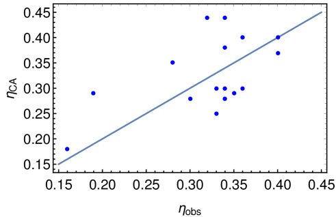
Figure 1: The observed efficiencies ($\eta_{\rm obs}$) of power plants, plotted relative to the CA-value for respective plants, as given in Ref. Johal (2017). A data point lying on the diagonal has the observed efficiency equal to CA-value. For data points above the diagonal, $\eta_{\rm obs}$ is below the CA-value, while the converse is true for the points below the diagonal.

Due to historical priority Vaudrey et al. (2014), the above expression is also addressed as Reitlinger-Chambadal-Novikov efficiency (see Box I). However, more recently it was rediscovered by Curzon and Ahlborn (CA) Curzon and Ahlborn (1975), and in the physics literature, it is popularly addressed as CA efficiency. For small differences in the reservoir temperatures, this formula yields the following behaviour:

$$\eta_{CA}\sim\frac{\eta_{C}}{2}+\frac{\eta_{C}^{2}}{8}+\cdots$$ (3)

So to first approximation, CA efficiency is “about” one-half of the Carnot value, which gives a reasonable estimate for the observed efficiencies of many actual plants (see Fig. 1).

In fact, CA expression for the efficiency can be derived by various different approaches and models. In this article, we highlight a few of the models which have been studied in recent years.

II CA efficiency with finite-time Carnot engine

The model proposed by Curzon and Ahlborn ascribes the only sources of irreversibilities to the finite rates of heat transfer across thermal resistances at both contacts with reservoirs (see Fig. 2). Further, it is assumed that the working medium remains in internal equilibrium at temperature $T_{1}<T_{h}(T_{2}>T_{c})$ while exchanging heat with the hot (cold) reservoir. Assuming a Newtonian flow of heat, the amount of heat flowing for time $t_{1}$ across the hot contact is:

$$Q_{h}=\alpha(T_{h}-T_{1})t_{1}.$$ (4)

Similarly, at the cold contact:

$$Q_{c}=\beta(T_{2}-T_{c})t_{2},$$ (5)

where $\alpha,\beta$ are the heat transfer coefficients. Thus, the work, $W=Q_{h}-Q_{c}$, is generated in time $t=t_{1}+t_{2}$. Note that the time for the adiabatic steps can be taken to be negligible by assuming fast relaxation times within the working medium.

An important assumption in this model is that the work generating compartment functions in a reversible way. This means that the working medium is in internal equilibrium, and this is called the endoreversible assumption, expressed as:

$$\frac{Q_{h}}{T_{1}}=\frac{Q_{c}}{T_{2}}.$$ (6)

Then, the average power output of the cycle, defined as $P=W/t$, may be optimized over the contact times ($t_{1},t_{2}$) Curzon and Ahlborn (1975), or alternately, over the intermediate temperature variables ($T_{1},T_{2}$). It is found that EMP is given by the CA formula, which, interestingly, is independent of the heat-transfer coefficients. Note that, obtaining the CA result here depends on the choice of the phenomenological heat transfer law. For instance, the choice of a different law gives a different expression for EMP, and so it is not quite general.

III Linear Irreversible model

There is another class of models, which do not consider a step-wise cycle of the working medium in a finite time. These models consider the fluxes of entropy, matter and energy in steady-state regime. The theoretical framework is based on Onsager theory Lebon et al. (2008) in which the fluxes ($J_{k}$) and their corresponding thermodynamic forces ($X_{k}$), or gradients, are identified. Applied to a heat engine between two heat reservoirs, suppose the engine performs work on the environment against a fixed external force $F$. Then the work output is $W=-Fx$, where $x$ is the conjugate variable of the force. The power output is written as $\dot{W}=-F\dot{x}$, where the dot represents the time derivative. Apart from the power flux, there is heat flux arising due to temperature gradient. Thus we can identify two flux-force pairs, as follows:

$$J_{1} = \dot{x},\quad X_{1}=\frac{F}{T},$$ (7)

$$J_{2} = \dot{Q}_{h},\quad X_{2}=\frac{\Delta T}{T^{2}},$$ (8)

where $T\approx T_{h}\approx T_{c}$, and $\Delta T=T_{h}-T_{c}$ is small compared to $T$. Then the rate of entropy generation can be written in a bilinear form:

$$\dot{S}=J_{1}X_{1}+J_{2}X_{2}.$$ (9)

In the limit of small gradients, each flux is assumed to be a linear combination of the available forces. Thus,

$$J_{1} = L_{11}X_{1}+L_{12}X_{2},$$ (10)

$$J_{2} = L_{21}X_{1}+L_{22}X_{2},$$ (11)

where the $L_{ij}$ are the phenomenological Onsager coefficients, satisfying the reciprocity relation, $L_{12}=L_{21}$. Then, the power can be written as

$$\dot{W}=-TJ_{1}X_{1}=-T(L_{11}X_{1}+L_{12}X_{2})X_{1}.$$ (12)

For given $X_{2}$, power may be optimized w.r.t $X_{1}$, which yields $X_{1}^{*}=-L_{12}X_{2}/2L_{11}$. Then the EMP, defined as $\eta^{*}=\dot{W}(X_{1}^{*})/\dot{Q}_{h}(X_{1}^{*})$, is evaluated to be:

$$\eta^{*}=\frac{\Delta T}{2T}\frac{q^{2}}{2-q^{2}}.$$ (13)

Here, $q=L_{12}/\sqrt{L_{11}L_{22}}$, denotes the strength of the coupling between the two fluxes, and satisfies $-1\leq q\leq+1$. At the tight-coupling condition $q^{2}=1$, we obtain the upper bound to EMP as $\Delta T/2T$, which is the half-Carnot value, or in other words, CA value is obtained to first approximation.

Thus, within the framework of linear irreversible thermodynamics, valid for small values of forces or gradients, and which assumes a linear dependence of fluxes on the forces, the EMP is bounded from above by $\eta_{\rm C}/2$ Van den Broeck (2005). Further, including conditions due to a certain left-right symmetry in the model, leads to the second order term of $\eta_{\rm C}^{2}/8$. Thus, although the CA formula—in its exact form—seems to be valid under more specific conditions, there is a universality of EMP upto second order, based on more general thermodynamic considerations.

Figure 2: Curzon Ahlborn model based on external irreversibilities, or the endoreversible assumption. The middle box represents the reversible, work-extracting compartment.

IV CA efficiency with a quasi-static model

IV.1 The case of complete information

Consider a textbook example Callen (1985) of two finite ideal-gas systems with a constant heat capacity $C$, at initial temperatures $T_{h}$ and $T_{c}$, which serve as our heat source and the sink in their initial states, respectively. We also assume the availability of heat reservoirs at fixed temperatures $T_{h}$ and $T_{c}$, by using which, the given systems may be prepared or brought to their initial states.

Now, the finite source and the sink are coupled to a reversible engine, which extracts maximal work due to the available temperature gradient. The total process will involve the two systems coming to mutual equilibrium at a common final temperature. Suppose, at an intermediate stage, the source has acquired a temperature $T_{1}$ while the sink is at temperature $T_{2}$. The amount of heat taken from the source by the engine is $Q_{\rm in}=C(T_{h}-T_{1})$, while the heat rejected to the sink is $Q_{\rm out}=C(T_{2}-T_{c})$. The process being reversible, the total entropy change in the two systems is zero. So, we have $\bigtriangleup S=C\ln{(T_{1}/T_{h})}+C\ln{(T_{2}/T_{c})}=0$. This yields the following relation between the final system temperatures

$$T_{1}=\frac{T_{h}T_{c}}{T_{2}}.$$ (14)

The extracted work, $W=Q_{\rm in}-Q_{\rm out}$, is given by

$$W=C(T_{h}+T_{c}-T_{1}-T_{2}).$$ (15)

Using Eq. (14), the efficiency $\eta=W/Q_{\rm in}$, can be written as:

$$\eta = 1-\frac{T_{c}}{T_{1}},$$ (16)

$$= 1-\frac{T_{2}}{T_{h}}.$$ (17)

We note that the work is maximum when the final temperatures of the systems are equal: $T_{1}=T_{2}=\sqrt{T_{h}T_{c}}$, and so the efficiency of the total process is $\eta_{\rm CA}$. Thus CA-efficiency emerges as the efficiency at maximum total work from finite ideal-gas systems.

For the curious reader, we wish to point out that by considering arbitrary thermodynamic systems as our source and sink, and possibly of different sizes, a general expression for efficiency can be derived Johal and Rai (2016). It also leads to the $\eta_{\rm C}/2$ result in the linear response regime, i.e. upto first order in temperature differences. When the sizes of the two systems are similar, it leads to the universal 1/8 factor in the second order term. Thus, we note that universality of efficiency, at maximum power (finite-time models), and at maximum work (quasi-static models), share similar features.

IV.2 Model with partial information

In the following, we introduce a completely different mechanism for arriving at CA efficiency. We shall first discuss the set-up, of finite-sized source and sink, from the point of view of a partial information and employ the methodology of inference (see Box II).

Now, from Eqs. (14) and (15), the work performed by our engine can be rewritten as

$$W(T_{2})=T_{h}+T_{c}-T_{2}-\frac{T_{h}T_{c}}{T_{2}}.$$ (18)

We let $C=1$, for simplicity. Clearly, a similar expression for work can be written in terms of $T_{1}$. So, just from the expression for work, it is not apparent as to which system (source or sink) the value $T_{2}$ belongs to. We have to look at the expression for the heat exchanged to assign a label corresponding to a specific system (in the above case, $T_{2}$ refers to the temperature of the sink). Clearly, in the standard thermodynamic model, the information conveyed by the symbol $T_{2}$, consists of two parts: i) the individual value of the temperature and ii) the label for the system to which it is assigned.

Now, suppose that we do not extract the maximal total work from the systems, but abort the process when the temperatures of one of the systems is $T$, and so, that of the other is $T_{h}T_{c}/T$. We imagine an observer who completes the cycle—bringing the systems back to their initial states by putting them in contact with respective reservoirs. In the case of an exact information, our observer makes no mistakes, and puts back the correct system with its respective reservoir. But, suppose, there is a probability of making an error in this last step. Maybe, the observer is careless and does not read the labels properly, or the labels may have got partially erased, and so on. Let us quantify the odds of this error with a probability, i.e a certain number $0\leq\gamma\leq 1$.

Now, given the above state of partial information, the task ahead of the observer is to make an estimate of the work performed, the efficiency of the process and so on. As mentioned above, the work expression does not reveal unambiguously the individual labels of the systems. Thus given one temperature value as $T$, the work expression will be written as: $W(T)=T_{h}+T_{c}-T-{T_{h}T_{c}}/{T}$.

To illustrate how the estimates may be based on our state of knowledge, suppose the observer is completely ignorant of the exact labels for the systems, which means he makes the maximal error, and given a system, he assigns equal probabilities that it may be the source or the sink, i.e., we assume $\gamma=1/2$. Then, the estimated temperature of each system can be given by the mean value over the two possible values:

$$\overline{T}=\frac{1}{2}\left(T+\frac{T_{h}T_{c}}{T}\right).$$ (19)

Now, we may estimate other quantities relevant to the performance of the engine. Our estimate of the heat absorbed by the engine is

$$Q_{\rm in}=T_{h}-\overline{T}.$$ (20)

Similarly, our estimate for the heat rejected to the sink will be:

$$Q_{\rm out}=\overline{T}-T_{c}.$$ (21)

The estimate for work, $W$, turns out to be the same, i.e. equal to the actual work performed, showing that the work is not affected by uncertainty in the labels of the final states of the systems.

For brevity, let us normalize all temperatures w.r.t to the initial temperature of the source, and define $\theta=T_{c}/T_{h}$ and $\tau=T/T_{h}$. So the estimate for work is

$$W(\tau)=1+\theta-\tau-\frac{\theta}{\tau}.$$ (22)

The estimate for the efficiency $\eta=W/Q_{\rm in}$ is then

$$\eta_{{1}/{2}}(\tau)=\frac{2(\tau+\theta\tau-\tau^{2}-\theta)}{2\tau-\tau^{2}-\theta}.$$ (23)

Now, if a given temperature value, $\tau$, actually belongs to the source, then the efficiency is: $\eta=1-\theta/\tau$, whereas if this value belongs to the sink, then $\eta=1-\tau$ (see Eqs. (16) and (17)). In the case of maximal error, the efficiency is as in Eq. (23).

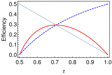
Figure 3: Plots of efficiency for $\theta=0.5$. $\tau$ takes values in the range $[\theta,1]$. Dashed curve is $\eta=1-\theta/\tau$, while the dotted curve is $\eta=1-\tau$. The solid curve is the estimate as in Eq. (23), whose maximal value is at $\tau=\sqrt{\theta}$ and is equal to CA value. Carnot limit is 0.5.

From Fig. 3, we see that in both cases of certainty about the labels (dotted and dashed curves), the maximum efficiency is the Carnot value ($1-\theta$). But, an uncertainty in the correct labels reduces the maximal efficiency below the Carnot value, which reduces to CA value in the case of maximal uncertainty. So, here we have a mechanism which shows how inference under partial information leads us to expect a lower value for the maximum efficiency obtainable in a heat engine. Thus, the upper bound for the efficiency is directly related to our state of knowledge and CA efficiency emerges from an entirely different perspective Johal et al. (2015).

Finally, we would like to illustrate the important role played by Bayes’ theorem (see Box III) in the theory of inference. Let us consider a two-level system with energy levels 0 and $a$, denoted by symbols ($\downarrow$) and ($\uparrow$), respectively. When we put this system in contact with a heat reservoir at a certain temperature $T$, the equilibrium Boltzmann distribution is given by $p(\uparrow|a)=1/(1+\exp(a/k_{B}T))$, and $p(\downarrow|a)=1-p(\uparrow|a)$. These probabilities can be regarded as conditional upon the given values of the energy gap $a$ and the temperature $T$. Now, suppose, we are ignorant about the exact value of the gap parameter $a$. So, instead we treat quantity $a$ as a random variable in the sense of subjective probability. We assign a prior distribution $\Pi(a)$, which for simplicity, may be taken as uniform density over some interval, $[0,a_{\rm max}]$, i.e. $\Pi(a)=1/a_{\rm max}$. Note that this range is to be based on some background information such as the permissible values (real positive, in this case) and the maximal gap that may be obtained in the laboratory or under given physical conditions, and so on. Let us now make a measurement on the system to know whether it is in the ground or excited state. Based on the result of the measurement, we can use Bayes’ theorem to update our probability for the gap as follows:

$$p(a|\uparrow)da=\frac{p(\uparrow|a)\Pi(a)da}{\int_{0}^{a_{\rm max}}p(\uparrow|a)\Pi(a)da},$$ (24)

which is a continuous-variable version, in contrast to the discrete case discussed in Box III. In order to appreciate the product form of the probabilities in the above equation, note that $\int p(\uparrow|a)\Pi(a)da\equiv p(\uparrow)$.

Now, initially, we have assumed all values of the gap to be equally likely (uniform prior). Then, upon measurement, if we find the system in ($\uparrow$) state, our revised guess or the posterior probabilities should assign more weight to smaller values of the gap, because these are more likely to cause the system to absorb energy from the reservoir and make it jump to ($\uparrow$) state. Otherwise, if the system is found in ($\downarrow$) state, then our posterior guess would be that the larger values of the gap are more likely. These inferences are illustrated in Fig. 4. Application of Bayes’ theorem in the above fashion to quantum heat cycles, where such a two-level system acts as a working medium, leads to the estimates of the work per cycle which becomes optimal at CA-efficiency, under certain conditions. Remarkably, this feature holds for a class of prior distributions Johal (2010).

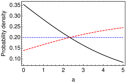
Figure 4: Probability density for the energy gap $a$ in two-level quantum system. Uniform prior is shown as dotted horizontal line. If the measurement shows the system in ($\uparrow$) state, the posterior density is given by solid line, indicating that the density becomes higher for smaller gap values. In case, the measurement shows ($\downarrow$) state, then the posterior density becomes higher for larger gaps (dashed line). Here, $a_{\rm max}=5$, temperature $T=2.5$, and $k_{B}=1$.

V Summary

Efficiency at maximum power output is an important figure of merit in the current research on nonequilibrium thermodynamics. Due to the simplicity and elegance of the CA formula, universal properties of the efficiency have been intensively studied in recent years. We have seen that CA value is obtained in a variety of models, ranging from finite time to quasi-static models of work extraction, including more abstract models of heat engines with partial thermodynamic information. Although other expressions for efficiency are also derived in different models, CA value provides an important benchmark against which these values may be compared, as, for instance, in the observed efficiencies of real power plants.

Box I: History of CA formula

The earliest known such model (1929) which derived the CA-efficiency, is ascribed to Reitlinger Reitlinger (2008). It involved a heat exchanger receiving heat from a finite hot stream fed by a combustion process. An analogous model (1957) was applied to a steam turbine by Chambadal Chambadal (1957). The considered heat exchanger in these models is effectively infinite. Novikov Novikov (1958) considered the heat transfer process (1958) between a hot stream and a finite heat exchanger with a given heat conductance. There are two simple, but significant assumptions used in these models: i) a constant specific heat of the inlet hot stream and ii) the validity of Newton’s law for heat transfer. Further, there appears a floating temperature-variable in between the highest and the lowest values, such as the temperature of the exhaust warm stream, over which the output power can be optimized. This yields an optimal value of the intermediate temperature which is usually found to be $\sqrt{T_{h}T_{c}}$, the geometric mean of $T_{h}$ and $T_{c}$. This leads directly to the result that the efficiency at maximum power is the CA value. The CA model (1975) Curzon and Ahlborn (1975), which was apprarently posed as a classroom problem, attracted the attention of the physics community and and it led to a new field termed as Finite-time Thermodynamics Andresen (2011). In the engineering literature, the analogous approach is called Entropy Generation Minimization Bejan (1996, 1997).

Box II: Prediction vs. Inference

It is important to appreciate the significance of inference in science, in general. Whereas prediction is concerned with the question of finding out the consequences when the causes are given, inference, on the other hand, deals with guessing the plausible causes, given the consequences. The questions of interest in the latter category, are also called inverse problems. For example, a traditional question may be to guess the diffraction pattern, given the size and shape of the aperture. But the corresponding question of inference would be that, given the pattern, one is required to guess the possible shape of the aperture. Inference is a useful tool when only a limited or partial information is available. Thus, another domain of inference is probability theory. A standard problem may be that given a certain proportion of black and white balls in a closed bag, what is the probability that a white ball will show up in the next draw? The problem of inference could be that the results of previous, finite number of draws are given and one is required to guess the proportion of white/black balls in the bag. Usually, inference is based on plausible reasoning, which makes a rational guess based on incomplete information, and arrives at the estimates for the uncertain quantities (see also Box III).

Box III: Bayes’ Theorem

In Bayesian approach to probability theory, all uncertainty is treated probabilistically. Thus, probability can be interpreted in a subjective sense—as the degree of rational belief of the observer based on his/her state of incomplete or partial knowledge about the system. A central role is played in this framework by the notion of prior probabilities, which reflect the state of background knowledge of the observer, before the data from observation is included in the analysis. Then, Bayes’ theorem is a tool by which the initial (prior) guess of probabilities for certain events/hypotheses is updated whenever a new piece of information or data is incorporated. To take a simple example, scientists may have some conjectures about the possibility of life on a certain planet, based on previous data. Then, suppose that the presence of water is discovered on this planet. Now, since water represents a distinct potential for life—as we know it, so the estimates of scientists about the existence of life on that planet are expected to change. Bayes’ theorem can be a useful tool here, if we are able to model its essential elements. More precisely, let $B$ represent the background knowledge before the discovery of water which is depicted as event $W$, and $L$ be the fact that life exists on the planet. Then $p(W|B)$ and $p(L|B)$ are the prior probabilities for the existence of water and life, respectively, on the planet. Similarly, $p(W|L,B)$ denotes the (conditional) probability for water, given that life exists there. Then, we are interested in $p(L|W,B)$, the updated or posterior probability for the existence of life, after water is discovered. This can be obtained from the product law of probabilities, i.e. $$p(L|W,B)p(W|B)=p(W|L,B)p(L|B).$$ (25) This is the essence of Bayes’ theorem, which takes into account how the new information updates our previous beliefs and their probabilities. Now, probabilities are numbers, which by definition, lie between zero and unity. Thus, an assignment of unit value implies certainty. In a specific scenario, we may assign $p(W|L,B)=1$, if we feel sure about the presence of water, in case, life is already known to exist. Then, we can conclude from the above that $p(L|W,B)>p(L|B)$. Thus our or scientists’ expectation about life on the planet increases, after the discovery of water.

References

- Curzon and Ahlborn (1975) F. L. Curzon and B. Ahlborn, Am. J. Phys. 43, 22 (1975).
- Bejan (1997) A. Bejan, Advanced Engineering Thermodynamics (Wiley, New York, 1997) p. 377.
- Esposito et al. (2010) M. Esposito, R. Kawai, K. Lindenberg, and C. Van den Broeck, Phys. Rev. Lett. 105, 150603 (2010).
- Johal (2017) R. S. Johal, The European Physical Journal Special Topics 226, 489 (2017).
- Vaudrey et al. (2014) A. Vaudrey, F. Lanzetta, and M. Feidt, J. Noneq. Therm. 39, 199 (2014).
- Reitlinger (2008) H. B. Reitlinger, Sur l’utilisation de la chaleur dans les machines á feu (”On the use of heat in steam engines”, in French). (Vaillant-Carmanne, Liége, Belgium, 2008).
- Chambadal (1957) P. Chambadal, Armand Colin, Paris, France 4, 1 (1957).
- Novikov (1958) I. Novikov, J. Nucl. Energy II 7, 125 (1958).
- Andresen (2011) B. Andresen, Ange. Chem. 50, 2690 (2011).
- Bejan (1996) A. Bejan, J. Appl. Phys. 79, 1191 (1996).
- Lebon et al. (2008) G. Lebon, D. Jou, and J. Casas-Vázquez, Understanding Non-equilibrium Thermodynamics: Foundations, Applications, Frontiers (Springer-Verlag, Berlin Heidelberg, 2008).
- Van den Broeck (2005) C. Van den Broeck, Phys. Rev. Lett. 95, 190602 (2005).
- Callen (1985) H. B. Callen, Thermodynamics and an Introduction to Thermostatistics, 2nd ed. (John Wiley, New York, 1985).
- Johal and Rai (2016) R. S. Johal and R. Rai, EPL (Europhys. Lett.) 113, 10006 (2016).
- Johal et al. (2015) R. S. Johal, R. Rai, and G. Mahler, Foundations of Physics 45, 158 (2015).
- Johal (2010) R. S. Johal, Phys. Rev. E 82, 061113 (2010).