On Robustness of Individualized Decision Rules

Abstract

With the emergence of precision medicine, estimating optimal individualized decision rules (IDRs) has attracted tremendous attention in many scientific areas. Most existing literature has focused on finding optimal IDRs that can maximize the expected outcome for each individual. Motivated by complex individualized decision making procedures and the popular conditional value at risk (CVaR) measure, we propose a new robust criterion to estimate optimal IDRs in order to control the average lower tail of the individuals’ outcomes. In addition to improving the individualized expected outcome, our proposed criterion takes risks into consideration, and thus the resulting IDRs can prevent adverse events. The optimal IDR under our criterion can be interpreted as the decision rule that maximizes the “worst-case” scenario of the individualized outcome when the underlying distribution is perturbed within a constrained set. An efficient non-convex optimization algorithm is proposed with convergence guarantees. We investigate theoretical properties for our estimated optimal IDRs under the proposed criterion such as consistency and finite sample error bounds. Simulation studies and a real data application are used to further demonstrate the robust performance of our methods. Several extensions of the proposed method are also discussed.

Keywords and Phrases: Conditional value at risk; Individualized decision rules; Non-convex optimization; Robustness; Tail controls

1 Introduction

Decision making is a long standing research problem in many scientific areas, ranging from engineering, management science, to statistics. In the era of big data, the traditional “one fits all” decision rules are no longer ideal in many applications due to data heterogeneity. A decision rule that works for certain individuals may not necessarily work for others. Motivated by this, it is desirable to make individualized decision rules (IDRs) that map from individual characteristics into available decision assignments. Developing effective IDRs has a wide range of applications. For example, a credit card company hopes to send a special offer for each targeted customer tailoring to their personal needs. An epidemiologist needs to decide whether to deliver a vaccine plan to a specific region in order to prevent the spread of diseases. In medical applications, IDRs can be developed for better prevention and treatment methods that are tailored to each individual patient. Developing optimal IDRs is one of the main goals of precision medicine, also known as personalized medicine.

Most existing methods in the literature, from the data analytic perspective, are focused on estimating the optimal IDR that can maximize the expected outcome or minimize the expected loss for each individual (Qian and Murphy 2011, Manski 2004). For example, we may want to learn an IDR $d$ that maps an individual’s covariate $\mathbf{X}\in{\cal X}$ into a binary decision space ${\cal A}=\{1,-1\}$, i.e., $d:{\cal X}\rightarrow{\cal A}$, in order to maximize the expectation of $R(d)$ or a utility function $u$ of $R(d)$. Here $R(d)$ is the random outcome under IDR $d$, which will be formally defined in Section 2. Then the problem can be mathematically formulated as the following optimization problem:

$$\max_{d\in{\cal D}_{0}}\hskip 12.0pt\mathbf{E}[R(d)],$$ (1)

where ${\cal D}_{0}$ is a class of all IDRs. If some utility function $u$ is used, then one could replace the objective function in (1) with $\mathbf{E}[u(R(d))]$. The equivalent form of Problem (1) is

$$\max_{t\in\mathbb{R},d\in{\cal D}_{0}} \hskip 12.0ptt$$ (2)

subject to $$\hskip 12.0ptt\leq\mathbf{E}[R(d)],$$

by using the hypographical representation (Rockafellar and Wets 2009).

According to (2), it may be reasonable to restrict the expected outcome larger than some threshold when stochastic ups and downs of outcome $R(d)$ can be safely averaged out. Then by implementing the IDR obtained by (2), we can guarantee on average the outcome will be at least as good as some threshold $t$. However, in practice, practitioners usually want to have a safe margin to protect against undesired outcomes, especially when the lower tails of the outcome are more important. For instance, in reliability engineering (Rockafellar and Royset 2010), people are often interested in controlling the failure probability of some designed systems or structures such as buildings and bridges, instead of expected failure time. Here the selection of designs can be interpreted as IDRs, which are based on environmental conditions, existing materials, etc. In precision medicine, sometimes the gain in the expected outcome may be very little by comparing two treatments while the tail of the potential outcome distribution is of direct interest (Wang et al. 2018). Suppose two drugs are used to improve CD4 T cell amount of AIDS patients. Since the normal range of CD4 cells is $500$-$1500$, then in practice the event of a certain subject $\{R_{i}(d)=600\}$ may be treated as good as the event of $\{R_{i}(d)=800\}$. In contrast, the event $\{R_{i}(d)=50\}$ may be considered much worse than $\{R_{i}(d)=400\}$. Hence only using (2) to search for the best IDR may not be sufficient when the tails are more important or the variability of the outcomes needs to be controlled. In this case, one may consider using the truncated mean with a fixed cutoff as a criterion for better decision making, i.e., $\mathbf{E}[\min(R(d),L)]$, where $L$ is a fixed cutoff. However, in general, the cutoff $L$ is unknown and can be difficult to determine. Even though $L$ can be pre-determined in some ideal case, when the scale of $R(d)$ is changed or there is some measurement error or batch effect in the observed $R_{i}(d)$, the final $L$ needs to be properly modified, which could still be hard to choose. In addition, for many applications especially medical studies, normal ranges are usually determined by quantiles of healthy people. Therefore it may be more reasonable to consider the expected outcome lower than a certain quantile when evaluating IDRs.

In this paper, motivated by the conditional value at risk (CVaR) used extensively in finance and risk management (Rockafellar and Uryasev 2000), we propose a new criterion that considers average lower tails of outcome to evaluate IDRs. The resulting IDR under our proposed criterion can optimize the outcome of each individual and provide a safe margin against adverse events jointly. Our work is closely related to the recent paper by Qi et al. 2019a, where they established a mathematical framework to study IDRs under general risk measures. In this work, we are more specific on the lower tail of outcomes for making decisions and develop a thorough statistical analysis. We propose an efficient optimization algorithm for our specific problem with better convergence guarantee than that of Qi et al. 2019a. In addition, several practical extensions are also discussed.

1.1 Related Literature

There is an increasing body of literature in learning optimal IDR under the framework of (1). The literature spans across various fields such as statistics, economics, and machine learning. Along the line of statistics literature, most existing methods can be roughly divided into two categories: model based methods and direct search methods. Q-learning (Watkins 1989, Murphy 2005, Schulte et al. 2014) and A-learning (Murphy 2003, Robins 2004, Shi et al. 2018) are two representative model based methods. Other variants include Fan et al. 2017, Gunter et al. 2011, etc. For direct search methods, by viewing IDR problems as a weighted classification problem, Zhao et al. 2012 proposed to use the weighted support vector machine method to estimate the optimal IDR. Following that, various types of machine learning methods were proposed, such as Liu et al. 2018, Zhou et al. 2017, Zhao et al. 2015, Cui et al. 2017, Tao and Wang 2017, Laber and Zhao 2015, Zhang et al. 2015, Chen et al. 2018, Zhang et al. 2020. In addition, Tian et al. 2014, Qi and Liu 2018 and Qi et al. 2019b proposed to use regression methods to directly estimate the optimal IDR. Recently, Wang et al. 2018 proposed to use the quantile of $R(d)$ as a criterion to search for best IDRs, which is closely related to this paper. Their method can help to obtain robust optimal IDRs by controlling the lower quantile. However, it can be unstable when the potential outcome distribution is discrete. More importantly, as we mentioned in the example of CD4 T cells, lower tails of the outcome should be treated differently: if both $\{R_{i}(d)=50\}$ and $\{R_{i}(d)=400\}$ are below the $25\%$ quantile, the first event should be considered much worse than the latter one. We will discuss this further in Section 2. Other quantile-based methods include Linn et al. 2017, Xiao et al. 2019 and Fang et al. 2021.

In the econometrics literature, Manski 2004 provided a comprehensive regret analysis on the estimation of optimal IDRs with some connection to statistical decision theory (Savage 1951). Later on, exact finite sample regret analysis was established by Stoye 2009 and Tetenov 2012. Under smooth parametric and semi-parametric settings, Hirano and Porter 2009 investigated asymptotic optimality and large sample properties of optimal IDRs. Other related work includes Chamberlain 2011, Bhattacharya and Dupas 2012, Kasy 2016. Recently, Kitagawa and Tetenov 2018 and Athey and Wager 2021 established rate-optimal regret bounds for learning optimal IDRs. All of these existing developments are based on expected outcome or expected utility. Dehejia 2008 studied the risk aversion of treatment effect evaluation by using the mean-variance trade off criterion.

We would like to point out the increasing literature of learning optimal IDRs in the machine learning community, which is often referred as batch learning from bandit feedback, such as Beygelzimer and Langford 2009, Dudík et al. 2011, Swaminathan and Joachims 2015, Dudík et al. 2011, Kallus 2018. Finally, in the reinforcement learning literature, CVaR has been used as constraints in Markov decision processes such as Tamar et al. 2015 and Chow et al. 2017.

1.2 Main Contributions and Outline

The main contributions of this paper can be summarized as follows. We leverage the CVaR criterion and propose a robust criterion to directly estimate the optimal IDR that can improve the expected outcome while simultaneously controlling the average lower tails of the outcome. We discuss several important properties of our criterion and its practical usage by providing safety protection for implementing optimal IDRs. An efficient non-convex optimization algorithm is proposed to compute the solutions with a convergence guarantee. We establish several important theoretical properties of our estimator under the proposed criterion similar to the regret analysis in Zhou et al. 2017, Athey and Wager 2021, where the difference is to handle additional estimation error due to the special structure of the CVaR criterion.

The remainder of this paper is organized as follows. In Section 2, supplementing the previous value function framework, we introduce a new criterion to estimate the optimal IDR by using the concept of CVaR in risk management. We present several properties of our proposed criterion. In Section 3, we discuss our statistical estimation procedure to compute optimal IDRs under our proposed criterion. An efficient non-convex optimization algorithm is presented by using some recent developments in difference of convex algorithms (DCA). In Section 4, we establish several important theoretical properties of our method based on statistical learning theory. We demonstrate our method via extensive simulation studies and a real data application in Sections 5. In Section 6, we discuss several extensions of our proposed criterion from the perspectives of algorithm and modeling. Some technical results are provided in the supplementary materials.

2 Robust Criteria to Estimate Optimal IDRs

2.1 Notation and Basic Settings

We discuss our IDR problem under the potential outcome framework (Rubin 1974). We use $R$ to denote the outcome after receiving treatment $A$. We consider a binary-treatment setting and encode $A$ as either $1$ or $-1$. The treatment space is denoted by ${\cal A}$, i.e., ${\cal A}=\left\{-1,1\right\}$. Let $\mathbf{X}\in{\cal X}$ denote the $p$-dimensional random vector for covariates. Here ${\cal X}\subset\mathbb{R}^{p}$ is the covariate space. Throughout this paper, we make the following three standard assumptions.

Assumption 2.1.

$R=R(A)$.

Assumption 2.2.

$R(a)\;\bot\;A\,|\,\mathbf{X}$ for any $a\in{\cal A}$, where $\bot$ represents independence.

Assumption 2.3.

$\pi(a|\mathbf{X})\geq c$ almost surely for any $a\in{\cal A}$ and some positive constant $c$.

For simplicity, we assume the random outcome $R$ has a bounded support. This assumption can be relaxed by the high-order moment condition. See Athey and Wager 2021 for more details. Without loss of generality, we assume that the larger $R$ indicates the better condition an individual is in. Throughout this paper, we consider a randomized experiment and therefore the propensity score $\pi(A|\mathbf{X})$ is known. For the observational studies, the proposed method can be applied as well by estimating the propensity score using various methods such as the logistic regression. An IDR $d$ is defined as a measurable function mapping from the covariate space ${\cal X}$ into the treatment space ${\cal A}$. We also let $L^{r}({\cal T},{\cal F}_{1},\mathbb{P})$ be the space of all measurable functions such that $\int_{T\in{\cal T}}|f(T)|^{r}\text{d}P^{d}<\infty$, where ${\cal F}_{1}$ is the $\sigma$-field generated by ${\cal T}:={\cal X}\times{\cal A}\times\mathbb{R}$ and $\mathbb{P}$ is the corresponding probability measure.

2.2 Expected Value Function Framework

Before introducing our new criterion and methods, we first present the value function framework used by the most existing methods, such as (Manski 2004) and (Qian and Murphy 2011). The value function of an IDR $d$ is defined as

$$V(d) =\mathbf{E}[R(d)]=\mathbf{E}_{\mathbf{X}}\left[\mathbf{E}[R(d)|\mathbf{X}]\right]=\mathbf{E}_{\mathbf{X}}\left[\mathbf{E}[R(d)|\mathbf{X},A=d(\mathbf{X})]\right]$$ (3)

$$=\mathbf{E}_{\mathbf{X}}\left[\mathbf{E}[R|\mathbf{X},A=d(\mathbf{X})]\right]=\mathbf{E}\left[\frac{R\mathbb{I}(A=d(\mathbf{X}))}{\pi(A|\mathbf{X})}\right],$$

where the first line is based on Assumption 2.2, the first equality in the second line is based on Assumption 2.1 and the last equality relies on Assumption 2.3. Based on this value function, an optimal IDR $d_{v}$ under the mean criterion is defined as

$$d_{v}\in\text{argmax}_{d\in{\cal D}_{0}}V(d),$$

which is equivalent to

$$d_{v}(\mathbf{X})\in\text{argmax}_{a\in{\cal A}}\,\mathbf{E}\left[R\,|\,\mathbf{X},A=a\right],$$

almost surely. It is observed that under the value function framework, the optimal IDR is to select the treatment with the largest expected outcome among all treatments for each individual.

Despite much progress towards developing optimal IDRs in the intersection of statistics, econometrics, and machine learning, only focusing on obtaining the largest expected outcome for each individual can be too restrictive and sometimes may not be even safe. For example, doctors may want to know whether a treatment does the best to improve the worst scenario, in particular for a patient with high risk. Without such a risk consideration, it may lead to serious consequences, such as exacerbation or hospitalization in practice. Similar concerns may happen in the credit card company, where the “best” policy should not only improve the expected profit, but also reduce the chance of incurring a heavy loss. This motivates us to control risk exposure associated with the corresponding decision rules, in addition to maximizing the expected outcome for each individual.

2.3 Conditional Value at Risk

It is natural to consider some robust metrics such as quantiles of $R$ given $\mathbf{X}$ and $A$ to measure the effect of a treatment (Wang et al. 2018). The corresponding optimal IDR $\widetilde{d}$ under the quantile may be defined as

$$\widetilde{d}\in\text{argmax}_{d\in{\cal D}_{0}}\,Q_{\gamma}(R(d)),$$ (4)

where $Q_{\gamma}(R(d))=\inf\{y:P(R(d)\leq y)\geq 1-\gamma\}$ and $\gamma\in(0,1)$. Analogous to Problems (1) and (2), an equivalent form of Problem (4) can be constructed as follows:

$$\max_{t\in\mathbb{R},d\in{\cal D}_{0}} \hskip 12.0ptt$$ (5)

subject to $$\hskip 12.0ptt\leq Q_{\gamma}(R(d)).$$

Based on the above representation, roughly speaking, the constraint set $\{t\leq Q_{\gamma}(R(d))\}$ implies that $(1-\gamma)\times 100\%$ of the population under the given IDR are controlled to be at least as good as a certain threshold $t$. Thus under the quantile criterion, one can obtain a robust IDR that can improve almost $(1-\gamma)\times 100\%$ of the population to some extent.

There are several potential drawbacks of using quantile in IDR problems. First of all, using the quantile criterion treats all the outcomes lower than $Q_{\gamma}(R(d))$ as the same. However, as we discussed in the aforementioned example, the CD4 T cell $\{R_{i}(d)=400\}$ below the normal level is considered to be much better than $\{R_{i}(d)=50\}$, therefore they should be treated differently in practice. Secondly, $Q_{\gamma}(R(d))$ is generally not continuous in $\gamma$, which may cause instability. For instance, if the outcome distribution is discrete and there is a small change in $\gamma$, the resulting optimal $\widetilde{d}$ may change significantly. Lastly, from the computational perspective, the quantile makes the optimization Problem (4) hard to solve and thus may limit its use in practice.

In order to address the drawbacks of using quantiles, we propose to use the conditional value at risk (CVaR), also known as expected tail loss, which was proposed by Artzner et al. 1999 in risk management. Consider a continuous random variable $Y$. Then the $\gamma$-CVaR of $Y$ may be defined as

$$S(F_{Y}):=\frac{1}{\gamma}\mathbf{E}[Y\mathbb{I}(Y\leq Q_{\gamma}(F_{Y}))],$$ (6)

where $F_{Y}$ is the corresponding probability distribution of $Y$. Based on this definition, the $\gamma$-CVaR can be interpreted as a truncated mean lower than $\gamma$-quantile of $Y$. For the general setting, instead of assuming a continuous distribution of $Y$, $\gamma$-CVaR is defined as an optimal value of a concave maximization problem by the celebrated work of Ben-Tal and Teboulle 1986, Rockafellar and Uryasev 2000, which is defined as follows:

$$S(F_{Y}):=\sup_{\alpha\in\mathbb{R}}\left\{\alpha-\frac{1}{\gamma}\mathbf{E}[(\alpha-Y)_{+}]\right\},$$ (7)

where $[t]_{+}=\max(0,t)$. The leftmost of the optimal solution set to (7) is $Q_{\gamma}(F_{Y})$ (Rockafellar and Uryasev, 2000,  Theorem 1). Then one can see that the definition in (7) is equivalent to (6) when the outcome distribution of $Y$ is continuous. We also remark that $Y$ is often referred to a loss in the finance literature. Here we call $Y$ an outcome/reward in order to be consistent with our problem setting.

Lastly, we would like to point out that $\gamma$-CVaR has several nice properties discussed by Artzner et al. 1999 and it is in general preferable to the quantile measure (Sarykalin et al. 2008). In particular, based on the interpretation of (6), $\gamma$-CVaR considers average outcomes lower than $\gamma$-quantile, which treats lower tails of outcome differently. This exactly satisfies our purpose. The concave maximization formulation in (7) demonstrates the continuity of $\gamma$-CVaR with respect to $\gamma$, which provides more stability measure compared with the quantile one. Furthermore, $\gamma$-CVaR is considered to be more computationally efficient than the quantile criterion because of the concave maximization formulation. Finally, Pflug 2000 and Rockafellar and Uryasev 2002 showed that $S(F_{Y})\leq Q_{\gamma}(F_{Y})$, suggesting that $\gamma$-CVaR is more conservative than $\gamma$-quantile. This also implies that a larger $\gamma$-CVaR of a random outcome indicates a larger $\gamma$-quantile. Clearly the reverse inequality does not necessarily hold. All these nice properties motivate us to use CVaR in the IDR problems. For the related theoretical discussion about CVaR, we refer to Rockafellar and Uryasev 2002 and the references therein.

2.4 A New Robust Criterion for IDR Problems

We borrow the concept of CVaR in order to conduct risk control to obtain a robust optimal IDR that can improve the lower tails of outcomes. Specifically, we define the following decision-rule based $\gamma$-CVaR criterion as

$$M_{0,\gamma}(d):=\sup_{\alpha\in\mathbb{R}}\left\{\alpha-\frac{1}{\gamma}\mathbf{E}[(\alpha-R(d))_{+}]\right\}.$$ (8)

Note that the difference between the criterion (8) and the original CVaR is to let the outcome $R$ depend on IDR $d$. The proposed criterion is not restricted to the continuous outcomes but can also be used in the discrete outcome cases, thus providing a broad application. In addition, if a small value of the outcome is more desirable (i.e., measuring the loss instead of the reward), one can replace $R(d)$ by $-R(d)$. All properties preserve. Given the coherent property of CVaR shown in Artzner et al. 1999, we have the following proposition for $M_{0,\gamma}(d)$.

Proposition 2.1.

The following properties of $M_{0,\gamma}(d)$ hold.

• If $R$ is shifted by a constant $c$, then $M_{0,\gamma}(d)$ is also shifted by the same constant $c$;

• If $R$ is multiplied by a positive constant $c$, then the corresponding $M_{0,\gamma}(d)$ is also multiplied by the same constant $c$;

• Given two IDRs $d_{1}$ and $d_{2}$, if $R(d_{1})\leq R(d_{2})$ almost surely, then

  $$M_{0,\gamma}(d_{1})\leq M_{0,\gamma}(d_{2});$$

• Given IDR $d$, $M_{0,\gamma}(d)\leq\min\{V(d),Q_{\gamma}(R(d))\}$.

In addition, if outcome $R=c$ almost surely, then $M_{0,\gamma}(d)=c$.

Remark 2.1.

Proposition (2.1) justifies the use of $M_{0,\gamma}(d)$. In particular, $(a)$ and $(b)$ demonstrate that $M_{0,\gamma}(d)$ is not affected by a constant shift or multiplication. $(c)$ implies that if one IDR is no worse than the other, $M_{0,\gamma}(d)$ preserves the preferences. The last property indicates that $M_{0,\gamma}(d)$ is more conservative than the expected outcome and the quantile criterion when evaluating an IDR $d$.

If the distribution of $R(d)$ is continuous, then we could rewrite (8) as

$$M_{0,\gamma}(d)=\frac{\mathbf{E}^{d}[R\mathbb{I}(R\leq Q_{\gamma}(R(d)))]}{\gamma}.$$ (9)

Note that

$$P(R(d)<\alpha)=\mathbf{E}[\sum_{a\in{\cal A}}\mathbb{I}(d(\mathbf{X})=a)P(R<\alpha|\mathbf{X},A=a)]=\mathbf{E}[P(R<\alpha|\mathbf{X},A=d(\mathbf{X}))].$$ (10)

Then $Q_{\gamma}(R(d))$ can be further expressed as

$$Q_{\gamma}(R(d))=\inf\left\{\alpha\,|\,\mathbf{E}[P(R<\alpha|\mathbf{X},A=d(\mathbf{X}))]\geq\gamma\right\},$$ (11)

which can be interpreted as the average $\gamma$-quantile of $R$ under the decision rule $d$. Correspondingly $M_{0,\gamma}(d)$ can be understood as the $\gamma$-average CVaR.

According to Proposition 2.1 (d), $M_{0,\gamma}(d)$ can be regarded as a lower bound of $V(d)$ and $Q_{\gamma}(R(d))$. Based on this, maximizing $M_{0,\gamma}(d)$ can thus potentially improve both $V(d)$ and $Q_{\gamma}(R(d))$. Then the optimal IDR under our proposed robust criterion $M_{0,\gamma}(d)$ is defined as

$$d_{0,\gamma}\in\text{argmax}_{d\in{\cal D}_{0}}\ M_{0,\gamma}(d).$$ (12)

The optimal IDR with respect to $M_{0,\gamma}(d)$ is to select a treatment/decision with the largest $\gamma$-average CVaR. Moreover, if we again use hypographical representation similar as those in (2) and (5), then we could formulate (12) as the following constraint optimization problem.

$$\max_{d\in{\cal D}_{0},t\in\mathbb{R}} \hskip 12.0ptt$$ (13)

subject to $$\hskip 12.0pt\sup_{\alpha\in\mathbb{R}}\left\{\alpha-\frac{1}{\gamma}\mathbf{E}[(\alpha-R(d))_{+}]\right\}\geq t.$$

Based on the formulation (13), $d_{0,\gamma}$ can be interpreted as the best IDR with the average lower tail of the outcome being at least as good as some certain threshold. Besides, based on statement (d) in Proposition (2.1), the constraint set in (13) implies $\min\{V(d),Q_{\gamma}(R(d))\}\geq t$. Therefore, by using $M_{0,\gamma}(d)$, the resulting optimal $d_{0,\gamma}$ can guarantee both $(1-\gamma)\times 100\%$ of the population’s outcomes and the expected outcome no worse than some threshold $t$.

By a similar derivation as that in (3), we have the following proposition.

Proposition 2.2.

$M_{0,\gamma}(d)=\sup_{\alpha\in\mathbb{R}}\left\{\alpha-\frac{1}{\gamma}\mathbf{E}[\frac{\mathbb{I}(A=d(\mathbf{X}))}{\pi(A|\mathbf{X})}(\alpha-R)_{+}]\right\}.$

The definition in (8) and Proposition (2.2) give us an efficient way to compute the optimal IDR $d_{0,\gamma}$ and $\alpha_{0}$ via jointly optimizing

$$(d_{0,\gamma},\alpha_{0})\in\underset{\alpha\in\mathbb{R},d\in{\cal D}_{0}}{\text{argmax}}\left\{\alpha-\frac{1}{\gamma}\mathbf{E}^{d}[(\alpha-R)_{+}]\right\}.$$ (14)

2.5 Dual Representation

Note that $M_{0,\gamma}(d)$ involves concave maximization with respect to $\alpha$. Thus it would be useful to investigate its dual representation by making use of convex duality theory in optimization (e.g., Rockafellar 1974). To begin with, we first define the following set:

$${\cal V}_{0}^{d}:=\{V\in L^{1}({\cal T},{\cal F}_{1},P^{d})\,|\,\mathbf{E}^{d}[V]=1,\,0\leq V(\omega)\leq\frac{1}{\gamma},\;\text{for}\;\omega\in{\cal T}\,\text{almost surely}\},$$

where $P^{d}$ is the probability measure under the IDR $d$. We have the following theorem that gives the dual representation of $M_{0,\gamma}(d)$.

Theorem 2.1.

$M_{0,\gamma}(d)=\inf_{V\in{\cal V}_{0}^{d}}\mathbf{E}^{d}[VR]$.

Dual representation of $M_{0,\gamma}(d)$: According to the dual representation of $M_{0,\gamma}(d)$ and its proof in the appendix, we can define a conditional probability measure $P^{\mathbf{V}}(B)=\int_{B}VdP^{d}$ for any measurable set $B\in{\cal F}_{1}$, where $V\in{\cal V}^{d}_{0}$. Then $V=\frac{dP^{\mathbf{V}}}{dP^{d}}$. Define

$$\zeta_{\gamma}(u)=\begin{cases}0&\text{if \ $0\leq u\leq\frac{1}{\gamma}$}\\ +\infty&\text{otherwise}\\ \end{cases}.$$

Then we can further rewrite $\mathbf{E}^{d}[VR]$ in $M_{0,\gamma}(d)$ as

$$\mathbf{E}^{d}[RV] =\mathbf{E}^{d}[R\frac{\text{d}P^{\mathbf{V}}}{\text{d}P^{d}}]+\mathbf{E}\left[\zeta_{\gamma}(\frac{\text{d}P^{\mathbf{V}}}{\text{d}P^{d}})\right]=\mathbf{E}_{\mathbf{X}}[\mathbf{E}_{P^{\mathbf{V}}_{|\mathbf{X}}}[R]]+\mathbf{E}_{\mathbf{X}}\left[\int\zeta_{\gamma}(\frac{dP^{\mathbf{V}}}{dP^{d}})dP^{d}\right]=\mathbf{E}_{P^{\mathbf{V}}}[R]+I_{\zeta_{\gamma}}(\frac{dP^{\mathbf{V}}}{dP^{d}}),$$

where $I_{\zeta_{\gamma}}(\cdot)$ can be interpreted as the $f$-divergence distance between $P^{\mathbf{V}}$ and $P^{d}$. Then $M_{0,\gamma}(d)=\inf_{P^{\mathbf{V}}\ll P^{d}}\mathbf{E}_{P^{\mathbf{V}}}[R]+I_{\zeta_{\gamma}}(\frac{dP^{\mathbf{V}}}{dP^{d}})$, where that $u\ll v$ denotes the probability measure $u$ is absolutely continuous with respect to the probability measure $v$. Thus the optimal IDR can also be written as

$$d_{0,\gamma}\in\text{argmax}_{d\in{\cal D}_{0}}\left\{\inf_{P^{\mathbf{V}}\ll P^{d}}\mathbf{E}_{P^{\mathbf{V}}}[R]+I_{\zeta_{\gamma}}(\frac{dP^{\mathbf{V}}}{dP^{d}})\ \right\},$$

which can be interpreted as choosing an optimal decision rule in terms of the worst expected outcome within the $f$-divergence distance from the original distribution $P^{d}$.

According to our problem setting, define the density under $P^{d}$ as $f_{0}(x)\mathbb{I}(d(x)=a)f_{1}(r|x,a)$. Since $P^{\mathbf{V}}\ll P^{d}$, then the density under $P^{\mathbf{V}}$ should be $v_{0}(x)\mathbb{I}(d(x)=a)v(r|x,a)$ for some conditional probability density $v_{0}(x)$ and $v_{1}(r|x,a)$. Then we have $\frac{dP^{\mathbf{V}}}{dP^{d}}=\frac{v_{0}(x)v_{1}(r|x,a=d(x))}{f_{0}(x)f_{1}(r|x,a=d(x))}$ by the chain rule. Therefore, we can further rewrite $M_{0,\gamma}(d)$ as

$$M_{0,\gamma}(d)=\inf_{P^{\mathbf{V}}}\left\{\mathbf{E}_{P^{\mathbf{V}}}[R]\,|\,P^{\mathbf{V}}\ll P^{d},\;0\leq\frac{v_{0}(\mathbf{X})v_{1}(r|\mathbf{X},a=d(\mathbf{X}))}{f_{0}(\mathbf{X})f_{1}(r|\mathbf{X},a=d(\mathbf{X}))}\leq\frac{1}{\gamma},\;\mbox{almost surely}\right\}.$$ (15)

This gives us a natural link to distributionally robust statistical models that can evaluate a decision rule under ambiguity. Maximizing $M_{0,\gamma}(d)$ over ${\cal D}_{0}$ is equivalent to identifying an optimal IDR that is robust to the contamination of both outcome $R$ and covariates $\mathbf{X}$ characterized by a probability constraint set. Recently, Mo et al. 2020 investigated distributionally robust ITRs by directly optimizing the expected rewards for the worse ITR within a perturbation set around the training distribution. Their method mainly focuses on potential covariate shifts. In contrast, by using a CVaR-based criterion, our proposed method is robust to distributional changes of both the outcome and covariates.

3 Statistical Estimation and Optimization

In this section, we discuss the estimation and optimization procedures for Problem (2.2) given observed data. The optimization in (14) can be rewritten as

$$\max_{\alpha\in\mathbb{R},d\in{\cal D}}\mathbf{E}[\frac{(\alpha-\frac{(\alpha-R)_{+}}{\gamma})\mathbb{I}(A=d(\mathbf{X}))}{\pi(A|\mathbf{X})}],$$

where ${\cal D}$ is some pre-specified classes of decision rules such as the linear ones. Consider the binary treatment setting and let $d(\mathbf{X})=\text{sign}(f(\mathbf{X}))$. Suppose we observe independently and identically distributed data $(\mathbf{X}_{i},A_{i},R_{i});i=1,\cdots,n$. Then we can estimate the optimal IDR via the empirical approximation:

$$\max_{\alpha\in\mathbb{R},d\in{\cal D}}\frac{1}{n}\sum_{i=1}^{n}\frac{\mathbb{I}(A_{i}=\text{sign}(f(\mathbf{X}_{i})))}{\pi(A_{i}|\mathbf{X}_{i})}(\alpha-\frac{(\alpha-R_{i})_{+}}{\gamma}).$$ (16)

It is well known that optimization over indicator functions is NP hard. Alternatively, similar to Zhou et al. 2017, we can replace the $0$-$1$ loss function by the following smooth truncated loss,

$$S(u)=\begin{cases}0&\text{if $u\leq-\delta$}\\ (1+u/\delta)^{2}/2&\text{if $0>u\geq-\delta$}\\ 1-(1-u/\delta)^{2}/2&\text{if $\delta>u\geq 0$}\\ 1&\text{if $u>\delta$},\end{cases}$$

and then use a functional margin representation to express $\mathbb{I}(A_{i}=\text{sign}(f(\mathbf{X}_{i}))$ as $\mathbb{I}(A_{i}f(\mathbf{X}_{i})>0)$ for each $i$. The corresponding function plot of $S(u)$ is shown in Figure 1 with $\delta=1$. From the plot, we can see that the smooth approximation $S(u)$ is very close to the $0$-$1$ loss. The parameter $\delta$ can control the closeness of this approximation. In practice, we can simply choose $\delta=1$.

Figure 1: Plot of the smooth surrogate loss function with $\delta=1$

By using the surrogate function, we can estimate the optimal IDR under $M_{0,\gamma}(d)$ via computing

$$\min_{\alpha\in\mathbb{R},f\in{\cal H}}\frac{1}{n}\sum_{i=1}^{n}\frac{S(A_{i}f(\mathbf{X}_{i}))}{\pi(A_{i}|\mathbf{X}_{i})}(-\alpha+\frac{(\alpha-R_{i})_{+}}{\gamma})+\frac{\lambda_{n}}{2}||f||^{2}_{{\cal H}},$$ (17)

where $||f||^{2}_{{\cal H}}$ is some convex penalty function on $f$. For example, if we consider ${\cal H}$ as a Reproducing Kernel Hilbert Space (RKHS), then $||f||^{2}_{{\cal H}}$ could be the square of the RKHS norm of $f$. The estimated IDR is given by $\hat{d}_{0,\gamma}(\mathbf{X})=\text{sign}(\hat{f}(\mathbf{X}))$. Note that Problem (17) involves a non-convex and potentially non-smooth optimization problem. Recent developments in difference-of-convex (DC) optimization (Pang et al. 2016) motivate us to use DC programming to efficiently solve this problem. Note that $S(u)$ can be expressed as a difference of convex differentiable functions: $S_{1}(u)-S_{2}(u)$, where

$$S_{1}(u)=\begin{cases}0&\text{if $u\leq-\delta$}\\ (1+u/\delta)^{2}/2&\text{if $-\delta<u\leq 0$}\\ 1/2+u/\delta&\text{if $0<u$}\\ \end{cases},$$

$$S_{2}(u)=\begin{cases}0&\text{if $u\leq 0$}\\ (u/\delta)^{2}/2&\text{if $0<u\leq\delta$}\\ u/\delta-1/2&\text{if $u>\delta$}\\ \end{cases}.$$

Define

$$G^{(1)}(f,\alpha):=\frac{1}{n}\sum_{i=1}^{n}\frac{S(A_{i}f(\mathbf{X}_{i}))}{\pi(A_{i}|\mathbf{X}_{i})}(-(\alpha-\frac{(\alpha-R_{i})_{+}}{\gamma}))+\frac{\lambda_{n}}{2}||f||^{2}_{{\cal H}},$$ (18)

and

$$G^{(1)}_{j}(f)=\frac{1}{n}\sum_{i=1}^{n}\frac{S(A_{i}f(\mathbf{X}_{i}))}{\pi(A_{i}|\mathbf{X}_{i})}(-R_{j}+\frac{(R_{j}-R_{i})_{+}}{\gamma}).$$ (19)

The following proposition gives us a way to express (17) as a DC function.

Proposition 3.1.

The following two optimization problems have the same optimal value, $i.e.$,

$$\min_{\alpha\in\mathbb{R},f\in{\cal H}}G^{(1)}(f,\alpha)=\min_{f\in{\cal H}}\left\{\widetilde{G}^{(1)}(f)\right\},$$ (20)

where $\widetilde{G}^{(1)}(f):=\min_{1\leq j\leq n}\{G^{(1)}_{j}(f)\}+\frac{\lambda}{2}||f||^{2}_{{\cal H}}$. More importantly, the optimal solution sets of $f$ to both problems are the same.

Based on Proposition 3.1, instead of solving (17), we can equivalently solve the optimization problem on the right hand side of (20). Let $c_{ij}=\frac{-(R_{j}-\frac{(R_{j}-R_{i})_{+}}{\gamma})}{\pi(A_{i}|\mathbf{X}_{i})}$ for $i=1,\cdots,n$ and $j=1,\cdots,n$, and note that $c_{ij}$ is not necessarily nonnegative. Recall that $S(u)=S_{1}(u)-S_{2}(u)$. We can further rewrite $G_{j}^{(1)}(f)$ as

$$G_{j}^{(1)}(f) =\frac{1}{n}\sum_{i=1}^{n}(\max(c_{ij},0)S_{1}(A_{i}f(\mathbf{X}_{i}))+\max(-c_{ij},0)S_{2}(A_{i}f(\mathbf{X}_{i})))$$

$$-\frac{1}{n}\sum_{i=1}^{n}(\max(c_{ij},0)S_{2}(A_{i}f(\mathbf{X}_{i}))+\max(-c_{ij},0)S_{1}(A_{i}f(\mathbf{X}_{i}))):=F_{j}(f)-H_{j}(f),$$

where both $F_{j}(f)$ and $H_{j}(f)$ are convex functions with respect to $f$ for $j=1,\cdots,n$. Then we can further decompose

$$\widetilde{G}^{(1)}(f)=\min_{1\leq j\leq n}\{F_{j}(f)-H_{j}(f)\}+\frac{\lambda}{2}||f||^{2}_{{\cal H}}$$

$$= \sum_{i=1}^{n}F_{j}(f)-\max_{1\leq j\leq n}\{H_{j}(f)+\sum_{k\neq j}^{n}F_{k}(f)\}+\frac{\lambda}{2}||f||^{2}_{{\cal H}}:= F(f)-\max_{1\leq j\leq n}h_{j}(f)+\frac{\lambda}{2}||f||^{2}_{{\cal H}},$$

as a DC function, where $h_{j}(f):=H_{j}(f)+\sum_{k\neq j}^{n}F_{k}(f)$. Note that $\widetilde{G}^{(1)}(f)$ is a potentially non-smooth function if there exits multiple $k$’s such that $h_{k}(f)=\max_{1\leq j\leq n}h_{j}(f)$. As discussed by Pang et al. 2016, traditional DC programming may converge to nonsense points. To address this issue, motivated by Pang et al. 2016, we define ${\cal M}_{\epsilon}(f):=\{j\ |\ h_{j}(f)\geq\max_{1\leq k\leq n}h_{k}(f)-\epsilon\}$, i.e., “$\epsilon$-argmax” index set, and use the following enhanced probabilistic DC algorithm summarized in Table 1 below to solve Problem (17).

Algorithm 1 Algorithm for solving (17)

1:Given a fixed $\epsilon>0$, let $f^{(v)}$ be the solution at the $v$ iteration for $v=1,2,\cdots$.

2:Randomly select $j\in{\cal M}_{\epsilon}(f^{(v)})$, and compute

$$f^{(v+1)}\in\text{argmin}_{f\in{\cal H}}\{F(f)-\frac{\partial h_{j}(f^{(v)})}{\partial f}(f-f^{(v)})+\frac{\lambda}{2}||f||^{2}_{{\cal H}}\}.$$ (21)

3:The algorithm stops when $|\widetilde{G}^{(1)}(f^{(v)})-\widetilde{G}^{(1)}(f^{(v+1)})|<\kappa$, for some pre-specified positive constant $\kappa$.

The proof of the convergence to sharp stationary points by the above algorithm can be found in Pang et al. 2016. For the computation of the subproblem (21), efficient algorithms such as the quasi-Newton method can be used. Compared with the algorithm proposed in Qi et al. 2019a, by using the surrogate loss, we avoid directly solving a discontinuous optimization problem. While Qi et al. 2019a transformed the problem into a constraint optimization by using the epigraph representation, it can be less efficient than our proposed algorithm as the number of constraints is proportional to the number of observations. In addition, the convergence to a shaper stationary point can be guaranteed by our algorithm. For a general treatment on non-convex and non-smooth optimization problems, we refer to Cui and Pang 2021.

4 Analysis of Statistical Convergence

In this section, we discuss the statistical theory related to our estimation under $M_{0,\gamma}(d)$. For the ease of presentation, we assume that Assumptions 2.1-2.3 always hold. With some abuse of notation, we first define

$$M_{0,\gamma}(d,\alpha)=\mathbf{E}[\frac{\mathbb{I}(A=d(\mathbf{X}))}{\pi(A|\mathbf{X})}(\alpha-\frac{1}{\gamma}(\alpha-R)_{+})],$$ (22)

and denote the optimal solution of maximizing (22) as $d_{0,\gamma}=\text{sign}(f_{0})$ and $\alpha_{0}$. Since we use the surrogate loss function $S(u)$, we further define

$$M_{S}(f,\alpha)=\mathbf{E}[\frac{S(Af(\mathbf{X}))}{\pi(A|\mathbf{X})}(\alpha-\frac{1}{\gamma}(\alpha-R)_{+})]$$

as the surrogate value function. Our theoretical results are similar to the standard regret analysis such as Zhou et al. 2017. The additional challenge is to handle the “nuisance” parameter $\alpha$, which requires additional efforts. For example, Fisher consistency cannot be directly obtained by using the standard proof such as that in Zhou et al. 2017.

4.1 Fisher Consistency

We first establish Fisher consistency of estimating optimal ITRs under $M_{S}(f,\alpha)$ to justify the use of the surrogate loss $S(u)$, compared with $M_{0,\gamma}(d,\alpha)$. The proof is different from the classical Fisher consistency in classification, which only involves one functional class of interest. Here we need to consider the effect of the surrogate function on estimating $\alpha$, which is thus more involved.

Theorem 4.1.

For any measurable function $f$ and $\alpha$ and a given $0<\gamma\leq 1$, if $(f_{S}^{\ast},\alpha_{S}^{\ast})$ maximizes $M_{S}(f,\alpha)$, then $(\text{sign}(f_{S}^{\ast}),\alpha_{S}^{\ast})$ maximizes $M_{0,\gamma}(d,\alpha)$.

Based on Theorem 4.1, instead of $M_{0,\gamma}(d,\alpha)$, we can target on $M_{S}(d,\alpha)$ equivalently.

4.2 Excess Value Bound

Based on Theorem 4.1, we can further justify the use of the surrogate function $S(u)$ by establishing the following excess value bound for the $0$-$1$ loss in $M_{0,\gamma}(d,\alpha)$.

Theorem 4.2.

For any measurable function $f,\alpha$ and any probability distribution over $(\mathbf{X},A,R)$,

$$M_{0,\gamma}(d_{0,\gamma},\alpha_{0})-M_{0,\gamma}(\text{sign}(f),\alpha)\leq 2(M_{S}(f_{S}^{\ast},\alpha_{S}^{\ast})-M_{S}(f,\alpha)).$$

Theorem 4.2 gives us a way of bounding the difference between the optimal IDR and the estimated IDR under $M_{0,\gamma}(d,\alpha)$ by using $M_{S}(d,\alpha)$ instead.

4.3 Convergence Rate

In order to obtain the finite sample performance of our estimated optimal IDR under $M_{0,\gamma}(d,\alpha)$, it is enough to focus on the difference of $M_{S}(d,\alpha)$ between the estimated optimal IDR and the optimal ITR based on Theorem 4.2. Define

$$(\hat{f},\hat{\alpha})=\text{argmin}_{f\in{\cal H},\alpha\in\mathbb{R}}O_{n}(f,\alpha)+\frac{\lambda_{n}}{2}||f||^{2}_{{\cal H}},$$ (23)

where $O_{n}(f,\alpha):=\frac{1}{n}\sum_{i=1}^{n}\frac{S(A_{i}f(\mathbf{X}_{i}))}{\pi(A_{i}|\mathbf{X}_{i})}(\frac{(\alpha-R_{i})_{+}}{\gamma}-\alpha)$. For simplicity, in the following we consider ${\cal H}$ be a RKHS. The results can be extended to other scenarios such as the class of linear functions with the $l_{1}$ penalty. Define $O_{T}(f,\alpha)=-M_{S}(f,\alpha)$ and let $(f_{\lambda_{n}},\alpha_{\lambda_{n}})=\text{argmin}_{f\in{\cal H},\alpha\in\mathbb{R}}O_{T}(f,\alpha)+\frac{\lambda_{n}}{2}||f||^{2}_{{\cal H}}.$ Then ${\cal A}(\lambda_{n}):=O_{T}(f_{\lambda_{n}},\alpha_{\lambda_{2n}})+\frac{\lambda_{n}}{2}||f_{\lambda_{n}}||^{2}_{{\cal H}}-O_{T}(f^{\ast}_{S},\alpha_{S}^{\ast})$ is considered to be the approximation error. The following theorem gives us a finite sample upper bound of our estimated optimal IDR and the optimal IDR based on $M_{0,\gamma}(d,\alpha)$.

Theorem 4.3.

For any distribution $P$ over $(\mathbf{X},A,R)$ such that the reward is uniformly bounded, i.e., $|R|\leq C_{0}$ for some positive constant $C_{0}$, if ${\cal A}(\lambda_{n})\leq C_{1}\lambda_{n}^{w_{1}}$, where $w_{1}\in(0,1]$, then with probability at least $1-\epsilon$,

$$M_{0,\gamma}(d_{0,\gamma},\alpha_{0})-M_{0,\gamma}(\text{sign}(\hat{f}),\hat{\alpha})\leq C_{2}n^{-\frac{w_{1}}{2w_{1}+1}},$$

for some positive constant $C_{2}$.

The above theorem shows that the difference between our estimated IDR and the optimal IDR under $M_{0,\gamma}(d,\alpha)$ converges to $0$ in probability under some conditions. The derivation requires additional control on the $\hat{\alpha}$, which can be shown to be uniformly bounded due to the optimization property. The upper bound assumption on the approximation error ${\cal A}(\lambda_{n})$ is analogous to those in the statistical learning literature such as Steinwart and Scovel 2007 to derive the convergence rate. The convergence rate is the same as those in Zhao et al. 2012 and Zhou et al. 2017. This is not surprising because the proposed $M_{0,\gamma}(d)$ can be roughly regarded as the truncated mean.

5 Numerical Studies

We conduct extensive simulation studies and real data analysis to illustrate the performance of our proposed method. For all simulation settings, we consider binary randomized trials with equal probabilities of patients being assigned to each treatment group. The performance will be similar when the difference in terms of the treatment assigned probabilities is not too large. In the extremely unbalanced case, the variance of the empirical approximation (17) could be large, which thus requires a large sample to achieve desired performance. For the ease of presentation, we only present results of estimated optimal IDRs under $M_{0,\gamma}(d)$ with the $l_{2}$ penalty on $f$ in Problem (17), where $f$ is a linear function of $\mathbf{X}$. We denote this method as $l2$-$\text{CVaR}_{\gamma}$.

All tuning parameters are selected based on the $10$-fold-cross-validation procedure. We select the tuning parameter that maximizes the empirical average of $M_{0,\gamma}(d)$ on the validation set. We compare our methods with the following four methods: (1) the $l_{1}$-PLS by Qian and Murphy 2011 with the basis function $(1,\mathbf{X},A,\mathbf{X}A)$; (2) the RWL by Zhou et al. 2017 with the linear kernel and the $l_{2}$ penalty. Note that RWL used the same truncated hinge loss as ours; (3) the $\gamma$-quantile optimal treatment regime denoted by $\text{IPWEQ}_{\gamma}$ (Wang et al. 2018); (4) the model-based $\gamma$-quantile regression for the optimal treatment regime denoted by $\text{QR}_{\gamma}$ (Linn et al. 2017, Xiao et al. 2019). All results are based on 100 replications.

Since we only consider the randomized design study where $A$ is either $1$ or $-1$ with equal probabilities, we do not compare those methods designed for observational studies such as (Zhang et al. 2012).

5.1 A Motivating Example

We use one toy example to demonstrate the necessity of tail control. In particular, the categorical covariate gender $X$ is generated by the uniform distribution over $\{1,-1\}$, where $1$ and $-1$ denote male and female respectively. Based on the randomly assigned treatment, the corresponding outcome $R$ is generated by the following model:

$$R=\mathbb{I}(XA=1)\epsilon_{1}+\mathbb{I}(XA=-1)\epsilon_{2},$$

where $\epsilon_{1}\sim{\cal N}(-0.1,1)$ and $\epsilon_{2}\sim{\cal N}(0,0.5)$. The corresponding plot is given in Figure 2. We consider training data with the sample size $n=200$ and independently generated test data of size $10000$. Based on test data, in Figure 3, we plot box plots of five different outcome distributions if treatments follow estimated IDRs by $l_{1}$-PLS, linear-RWL, $\text{IPWEQ}_{0.5}$, $\text{QR}_{0.5}$, and $l2$-$\text{CVaR}_{0.5}$, respectively. Based on these box plots, we can observe that since there is not much difference between these two treatments based on the expected outcome, the empirical mean of value functions resulted from these five methods are indistinguishable. However, besides improving the expected or median outcome for each individual, our methods also control the tails of individuals, thus prefer treatments with less variability. The resulting outcome distribution by our method is more stable, and thus has less variability than the other four methods. If we choose different $\gamma$ for $\text{IPWEQ}_{\gamma}$ and $\text{QR}_{\gamma}$, e.g., 0.25, their resulting outcome distributions will be similar to ours since they focus more on the tail like our proposed method.

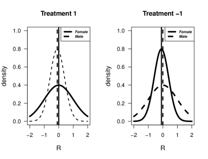
Figure 2: Plots of a motivating example. The dash and solid lines in the left plot show the probability densities of ${\cal N}(-0.1,0.5)$ and ${\cal N}(0,1)$ respectively. The dash and solid lines in the right plot correspond to the probability densities of ${\cal N}(0,1)$ and ${\cal N}(-0.1,0.5)$ respectively.

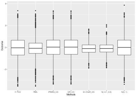
Figure 3: Box plots of value functions computed by five methods and two reference distributions. Methods starting from left to right are $l_{1}$-PLS, linear RWL, $\text{IPWEQ}_{0.5}$ $\text{QR}_{0.5}$, $l2$-$\text{CVaR}_{0.5}$ respectively. The last two box plots correspond to two reference normal distributions, i.e., ${\cal N}(-0.1,0.5)$ and ${\cal N}(0,1)$.

5.2 An illustrative Example

To further illustrate how our proposed method differs from the mean and quantile optimal treatment regimes, we consider another simulating example, motivated by Wang et al. 2018. Consider the reward $R=1+X+(3-5X)A+(1+A+2AX)\epsilon$, where $\epsilon\sim{\cal N}(0,1)$ and $X\sim\text{uniform}(0,1)$. We implement the above mentioned five methods with $\gamma=0.1,0.25,0.5$ using $50000$ observations. Then we report their performance on $10^{6}$ testing observations under different criteria in Table 1. As expected, methods perform the best under their corresponding criteria. For the $\text{QR}_{\gamma}$ method, while the goal is to find the best treatment with the largest conditional quantile treatment effect, it is not necessary to maximize the population quantile, i.e., $Q_{\gamma}(R(d))$. But their performances are also robust. In general, under the mean evaluation criterion, since our proposed methods focus on outcomes lower than certain quantiles, the performances are not as good as those mean-optimal treatment regimes, especially when $\gamma$ is small. However, when the evaluating criterion is on the low tails of outcomes, our methods are the most robust among all compared methods as $M_{0,\gamma}(d)\leq\min\{V(d),Q_{\gamma}(R(d))\}$. Furthermore, based on the reported coefficients of all estimated IDRs, it seems that robust IDRs given by our methods (or quantile based methods) tend to assign the treatment $A=-1$ as the majority treatment as it is better in improving lower tails of the outcome. Here we normalize the coefficients of IDRs so that all intercepts equal to $1$.

Table 1: Mean, different quantiles, and CVaR of the outcomes under 11 different treatment regimes given by different methods. The last two rows are the corresponding optimal IDRs’ coefficients.

Criterion	$l_{1}$PLS	RWL	$\text{IPWEQ}_{0.5}$	$\text{IPWEQ}_{0.25}$	$\text{IPWEQ}_{0.1}$	$\text{QR}_{0.5}$	$\text{QR}_{0.25}$	$\text{QR}_{0.1}$	$l2$$\text{CVaR}_{0.5}$	$l2$$\text{CVaR}_{0.25}$	$l2$$\text{CVaR}_{0.1}$
Mean	2.802	2.803	2.747	2.798	2.721	2.803	2.707	2.46	2.761	2.684	2.499
$Q_{0.5}$	2.81	2.801	2.853	2.761	2.594	2.797	2.569	2.233	2.666	2.532	2.281
$Q_{0.25}$	1.32	1.325	1.191	1.331	1.246	1.326	1.226	0.891	1.296	1.197	0.943
$Q_{0.1}$	-0.153	-0.116	-0.566	-0.018	0.119	-0.106	0.119	-0.037	0.094	0.118	-0.002
$\text{CVaR}_{0.5}$	0.932	0.947	0.727	0.985	0.997	0.952	0.988	0.766	1.011	0.974	0.806
$\text{CVaR}_{0.25}$	-0.231	-0.197	-0.614	-0.099	0.066	-0.187	0.071	-0.024	0.026	0.079	0.004
$\text{CVaR}_{0.1}$	-1.594	-1.535	-2.179	-1.355	-0.944	-1.516	-0.912	-0.744	-1.076	-0.864	-0.744
Opt. IDR	$l_{1}$-PLS	RWL	$\text{IPWEQ}_{0.5}$	$\text{IPWEQ}_{0.25}$	$\text{IPWEQ}_{0.1}$	$\text{QR}_{0.5}$	$\text{QR}_{0.25}$	$\text{QR}_{0.1}$	$\text{CVaR}_{0.5}$	$\text{CVaR}_{0.25}$	$\text{CVaR}_{0.1}$
intercept	1	1	1	1	1	1	1	1	1	1	1
coefficient	-1.635	-1.663	-1.420	-1.759	-2.115	-1.672	-2.165	2.959	-1.965	-2.241	-2.831

5.3 Distributional Shift Examples

Next we demonstrate the superior performance of our methods under distributional shifts of both covariates $\mathbf{X}$ and outcome $R$ based on the dual representations of $M_{0,\gamma}(d)$ in (15). Since (15) is related to the expected outcome under some class of distributions, we only compare with mean-optimal IDRs such as $l_{1}$-PLS and RWL. For the purpose of illustration, we only consider the sample size $n=200$ and the dimension $p=20$. The outcome $R$ is generated by the model: $R=1+X_{1}+X_{2}+A(X_{1}-X_{2}+X_{3})+\epsilon$. We consider the following two distributional shift scenarios:

• Each training covariate follows a two-component Gaussian mixture distribution of ${\cal N}(0,1)$ and asymmetric log-normal distribution $lognorm(0,2)$ with probabilities of the two mixture components to be $0.7$ and $0.3$ respectively and $\epsilon$ follows the standard Gaussian distribution. Each test covariate and the test $\epsilon$ follow the standard Gaussian distribution.

• Covariates $X$ are generated by the uniform distribution between $-1$ and $1$ and $\epsilon$ follows a two-component mixture distribution of ${\cal N}(0,1)$ and asymmetric log-normal distribution $lognorm(0,2)$ with probabilities of the two mixture component to be $0.7$ and $0.3$ respectively. For the test data, covariates X follow uniform distribution from $-1$ to $1$ and the test $\epsilon$ follows the standard Gaussian distribution.

The first scenario considers the covariate distributional shift and the second scenario considers the outcome distributional shift. For simplicity, we only report misclassification error rates given by $l_{1}$-PLS, RWL and $l2$-$\text{CVaR}_{0.5}$ in Table 2. For Scenario (1), since $l_{1}$-PLS assumes a linear model, its performance is not affected by the distributional shift of covariates. In contrast, RWL, which is based on maximizing the value function, depends heavily on correct approximations to the value function empirically. Thus the performance of RWL is worse than $l_{1}$-PLS under this scenario. For the estimated optimal IDR under our proposed $M_{0,\gamma}(d)$, the performance is superior to RWL because $M_{0,\gamma}(d)$ considers the perturbation of the covariate distributional shift. For Scenario (2), since the estimated optimal IDR under $M_{0,\gamma}(d)$ is a minimax estimator under the outcome distributional shift, the performance is much better than the other two methods developed under the value function framework.

Table 2: Comparisons of misclassification error rates (standard deviations) for simulated examples with $n=200$ and $p=20$.

	Scenario (1)	Scenario (2)
$l_{1}$-PLS	0.07 (0.01)	0.41 (0.007)
RWL	0.14 (0.006)	0.40 (0.008)
$l2$-$\text{CVaR}_{0.5}$	0.08 (0.01)	0.19 (0.004)

5.4 Additional Simulation Scenarios

We further study the performance of our proposed methods via three additional simulation examples, where the treatment-covariate interactions are linear. Nonlinear scenarios can be found in the supplementary material. We consider different combinations of $n$ and $p$, i.e., $n=500,1000$ and $p=5,10,20$, respectively. For the ease of presentation, we only present results of $n=1000$ and $p=10$ since it is close to our real data size. Other results can be found in the Supplementary material. We consider covariates $\mathbf{X}$ generated by the uniform distribution between $-1$ and $1$. The outcome $R$ is generated by the model: $R=m(\mathbf{X})+A\delta(\mathbf{X})+\epsilon$. We consider the following three different combinations of $m(\mathbf{X})$, $\delta(\mathbf{X})$ and $\epsilon$:

• $m(\mathbf{X})=1+X_{1}+X_{2}$, $\delta(\mathbf{X})=X_{1}-X_{2}+X_{3}$, and $\epsilon\sim{\cal N}(0,2)$;

• $m(\mathbf{X})=1+X_{1}+X_{2}$, $\delta(\mathbf{X})=X_{1}-X_{2}+X_{3}$, and $\log(\epsilon)\sim{\cal N}(0,1)$;

• $m(\mathbf{X})=1+X_{1}+X_{2}+X_{3}+X_{4}$, $\delta(\mathbf{X})=\exp(2X_{1})(-1+X_{1}-X_{2}+X_{3})$, and $\log(\epsilon)\sim{\cal N}(0,2)$.

In the first scenario, we consider the standard normal error distribution. This setting is oracle for $l_{1}$-PLS and $\text{QR}_{0.5}$. The second scenario considers the error generated by log-normal distribution, which has a heavy right tail. This setting is used to test the robustness of different IDRs and is oracle for $\text{QR}_{\gamma}$. The last setting is used to show the advantage of direct methods over model-based methods when the model is misspecified but the decision function is correctly specified. In addition, this scenario considers the same error distribution as the second one. Note that in all these three scenarios, the treatment only interacts with $\delta(\mathbf{X})$ in the mean model. Therefore the global optimal decision rule is always $\text{sign}(\delta(\mathbf{X}))$.

For our proposed method, $\text{IPWEQ}_{\gamma}$ and $\text{QR}_{\gamma}$, three different $\gamma$’s, i.e., $\gamma=0.1,0.25,0.5$. are considered. In order to evaluate different methods, we generate test data and compute mean, different quantiles and CVaRs on the test data under all estimated IDRs. More results can be found in Supplementary material. Since the global optimal IDR is known, i.e., $\text{sign}(\delta(\mathbf{X}))$, we can compute misclassification error rates for different methods on the test data, denoted by overall-error-rate in all tables below. In addition, to further show the robustness of different IDRs, we also compute the upper-error-rate and lower-error-rate. The upper-error-rate refers to misclassification error of observations with outcomes larger than $90\%$ quantiles and the lower-error-rate is for observations with outcomes smaller than $10\%$ quantiles. The results are summarized in Tables 3-5. Overall, our methods show competitive performances among all methods. In particular, for Scenario (1), which is the standard simulation setting in the literature, our proposed methods performs well in finding optimal IDRs, despite the slightly worse performance than mean-optimal IDRs. Since we focus more on the lower-tail, this is not surprising. For Scenario (2), as the error distribution is heavily right-tailed, methods under the value function framework ignore individuals with potentially high risks, i.e., outcome lower than the threshold, while only focusing on maximizing the value function. Therefore the resulting performances could be worse than robust methods. Among three robust methods, $\text{QR}_{\gamma}$ performs the best as it is oracle in this scenario. It can also be seen that our method performs better than that of Wang et al. 2018 in improving outcomes of lower tails. One potential reason is due to the optimization instability in training $\text{IPWEQ}_{\gamma}$. In terms of misclassification errors, all robust methods have smaller lower-error-rates than mean-optimal methods, demonstrating the superior performance of these estimated IDRs on the individuals with poor outcomes. In addition, we can observe that our method is more accurate than $\text{IPWEQ}_{\gamma}$ in identifying optimal treatments for individuals with small outcomes. For Scenario (3), our method performs the best among all methods. This is not surprising as our method does not model the outcome directly and thus does not suffer from model misspecification like $\text{QR}_{\gamma}$. In addition, our method is more robust than those under the value function framework, thus shows better empirical performance in this setting. Note that $\text{IPWEQ}_{\gamma}$ performs similar to ours as it is also a direct method.

Table 3: Setting 1 with $n=1000$ and $p=10$. Mean, different quantiles, and CVaR of the outcomes under 11 different treatment regimes given by different methods are reported. The corresponding standard errors are in the parentheses.

Criterion	$l_{1}$-PLS	RWL	$\text{IPWEQ}_{0.5}$	$\text{IPWEQ}_{0.25}$	$\text{IPWEQ}_{0.10}$
mean	2.162(0.002)	2.152(0.003)	2.081(0.011)	2.108(0.009)	2.11(0.008)
$Q_{0.5}$	2.151(0.001)	2.141(0.002)	2.089(0.009)	2.107(0.007)	2.107(0.007)
$Q_{0.1}$	0.192(0.006)	0.175(0.005)	0.016(0.026)	0.079(0.021)	0.088(0.016)
$\text{CVaR}_{0.5}$	0.931(0.004)	0.916(0.004)	0.798(0.019)	0.843(0.015)	0.849(0.012)
$\text{CVaR}_{0.1}$	-0.482(0.008)	-0.5(0.007)	-0.718(0.038)	-0.63(0.028)	-0.611(0.02)
overall-error-rate	0.029(0.005)	0.05(0.004)	0.117(0.008)	0.097(0.008)	0.095(0.006)
upper-error-rate	0.006(0.001)	0.014(0.002)	0.032(0.003)	0.027(0.003)	0.029(0.003)
lower-error-rate	0.01(0.002)	0.013(0.001)	0.049(0.007)	0.034(0.005)	0.03(0.003)
Criterion	$\text{QR}_{0.5}$	$\text{QR}_{0.25}$	$\text{QR}_{0.1}$	$l2$-$\text{CVaR}_{0.5}$	$l2$-$\text{CVaR}_{0.25}$	$l2$-$\text{CVaR}_{0.1}$
mean	2.163(0.001)	2.163(0.001)	2.16(0.001)	2.143(0.004)	2.141(0.004)	2.131(0.007)
$Q_{0.5}$	2.151(0.001)	2.15(0.001)	2.148(0.001)	2.135(0.004)	2.132(0.004)	2.124(0.006)
$Q_{0.1}$	0.199(0.001)	0.197(0.002)	0.191(0.002)	0.156(0.01)	0.15(0.009)	0.132(0.014)
$\text{CVaR}_{0.5}$	0.935(0.001)	0.933(0.001)	0.929(0.002)	0.902(0.007)	0.897(0.007)	0.883(0.011)
$\text{CVaR}_{0.1}$	-0.47(0.002)	-0.473(0.002)	-0.481(0.004)	-0.527(0.013)	-0.532(0.011)	-0.551(0.016)
overall-error-rate	0.026(0.002)	0.028(0.002)	0.035(0.002)	0.061(0.006)	0.065(0.005)	0.075(0.006)
upper-error-rate	0.007(0.001)	0.008(0.001)	0.009(0.001)	0.016(0.002)	0.017(0.002)	0.022(0.003)
lower-error-rate	0.007(0.001)	0.008(0.001)	0.01(0.001)	0.018(0.002)	0.019(0.002)	0.02(0.002)

Table 4: Setting 2 with $n=1000$ and $p=10$. Mean, different quantiles, and CVaR of the outcomes under 11 different treatment regimes given by different methods are reported. The corresponding standard errors are in the parentheses.

Criterion	$l_{1}$-PLS	RWL	$\text{IPWEQ}_{0.5}$	$\text{IPWEQ}_{0.25}$	$\text{IPWEQ}_{0.10}$
mean	8.875(0.122)	8.933(0.106)	9.316(0.029)	9.42(0.017)	9.459(0.01)
$Q_{0.5}$	3.208(0.107)	3.268(0.092)	3.574(0.011)	3.62(0.006)	3.635(0.004)
$\text{CVaR}_{0.5}$	1.454(0.136)	1.514(0.119)	1.961(0.034)	2.094(0.02)	2.148(0.012)
$\text{CVaR}_{0.1}$	-0.337(0.187)	-0.301(0.157)	0.281(0.084)	0.559(0.049)	0.686(0.027)
overall-error-rate	0.336(0.039)	0.318(0.034)	0.18(0.012)	0.127(0.009)	0.099(0.007)
upper-error-rate	0.334(0.039)	0.317(0.034)	0.177(0.011)	0.125(0.009)	0.098(0.007)
lower-error-rate	0.265(0.06)	0.247(0.052)	0.096(0.019)	0.047(0.01)	0.027(0.005)
Criterion	$\text{QR}_{0.5}$	$\text{QR}_{0.25}$	$\text{QR}_{0.1}$	$l2$-$\text{CVaR}_{0.5}$	$l2$-$\text{CVaR}_{0.25}$	$l2$-$\text{CVaR}_{0.1}$
mean	9.504(0.006)	9.512(0.003)	9.507(0.002)	9.485(0.008)	9.502(0.006)	9.501(0.006)
$Q_{0.5}$	3.656(0.001)	3.662(0)	3.663(0)	3.647(0.003)	3.652(0.002)	3.651(0.002)
$Q_{0.1}$	1.405(0.001)	1.408(0)	1.335(0.011)	1.363(0.007)	1.364(0.007)	1.364(0.007)
$\text{CVaR}_{0.5}$	2.21(0.003)	2.231(0)	2.233(0)	2.183(0.007)	2.201(0.005)	2.2(0.005)
$\text{CVaR}_{0.1}$	0.818(0.008)	0.861(0.001)	0.865(0)	0.76(0.016)	0.797(0.011)	0.798(0.01)
overall-error-rate	0.051(0.004)	0.014(0.001)	0.006(0)	0.077(0.006)	0.062(0.005)	0.063(0.005)
upper-error-rate	0.051(0.004)	0.014(0.001)	0.006(0)	0.076(0.006)	0.061(0.005)	0.063(0.005)
lower-error-rate	0.01(0.002)	0.003(0)	0.001(0)	0.015(0.003)	0.011(0.002)	0.011(0.002)

Table 5: Setting 3 with $n=1000$ and $p=10$. Mean, different quantiles, and CVaR of the outcomes under 11 different treatment regimes given by different methods are reported. The corresponding standard errors are in the parentheses.

Criterion	$l_{1}$-PLS	RWL	$\text{IPWEQ}_{0.5}$	$\text{IPWEQ}_{0.25}$	$\text{IPWEQ}_{0.10}$
mean	9.228(0.232)	9.302(0.208)	10.123(0.11)	10.351(0.034)	10.355(0.03)
$Q_{0.5}$	3.439(0.152)	3.511(0.132)	4.074(0.069)	4.227(0.023)	4.232(0.02)
$Q_{0.1}$	-0.177(0.264)	-0.144(0.254)	0.738(0.141)	1.023(0.048)	1.044(0.037)
$\text{CVaR}_{0.5}$	0.924(0.239)	0.967(0.221)	1.845(0.128)	2.12(0.046)	2.138(0.037)
$\text{CVaR}_{0.1}$	-2.555(0.564)	-2.544(0.522)	-0.519(0.312)	0.138(0.115)	0.191(0.094)
overall-error-rate	0.348(0.041)	0.333(0.037)	0.168(0.026)	0.102(0.013)	0.098(0.011)
upper-error-rate	0.34(0.042)	0.322(0.038)	0.155(0.024)	0.094(0.012)	0.09(0.01)
lower-error-rate	0.28(0.055)	0.278(0.053)	0.09(0.031)	0.028(0.011)	0.023(0.009)
Criterion	$\text{QR}_{0.5}$	$\text{QR}_{0.25}$	$\text{QR}_{0.1}$	$l2$-$\text{CVaR}_{0.5}$	$l2$-$\text{CVaR}_{0.25}$	$l2$-$\text{CVaR}_{0.1}$
mean	10.01(0.032)	10.034(0.022)	10.014(0.033)	10.419(0.018)	10.427(0.017)	10.424(0.013)
$Q_{0.5}$	4(0.02)	4.002(0.015)	4.004(0.021)	4.291(0.013)	4.296(0.011)	4.29(0.01)
$Q_{0.1}$	0.602(0.034)	0.633(0.023)	0.605(0.036)	1.137(0.029)	1.151(0.026)	1.142(0.021)
$\text{CVaR}_{0.5}$	1.707(0.035)	1.734(0.024)	1.711(0.036)	2.23(0.026)	2.242(0.024)	2.235(0.018)
$\text{CVaR}_{0.1}$	-0.851(0.091)	-0.746(0.058)	-0.849(0.092)	0.379(0.067)	0.408(0.059)	0.4(0.041)
overall-error-rate	0.208(0.007)	0.208(0.005)	0.207(0.007)	0.059(0.009)	0.053(0.008)	0.058(0.008)
upper-error-rate	0.19(0.006)	0.191(0.005)	0.189(0.007)	0.054(0.008)	0.049(0.008)	0.054(0.007)
lower-error-rate	0.12(0.009)	0.11(0.006)	0.12(0.009)	0.008(0.006)	0.006(0.005)	0.006(0.003)

5.5 Real Data Applications

We perform a real data analysis to further evaluate our proposed robust criterion for estimating optimal IDRs. We use the clinical trial dataset from “AIDS Clinical Trials Group (ACTG) 175” in Hammer et al. 1996 to study whether there exists some subpopulations that are suitable for different combinations of treatments for AIDS. In this study, a total number of $2139$ patients with HIV infection is randomly assigned into four treatment groups: zidovudine (ZDV) monotherapy, ZDV combined with didanosine (ddI), ZDV combined with zalcitabine (ZAL), and ddI monotherapy with equal probabilities. In this data application, we focus on finding optimal IDRs between two treatments: ZDV with ddI and ZDV with ZAL as our interest. The total number of patients receiving these two treatments is 1046.

Similar to the previous studies by Lu et al. 2013 and Fan et al. 2017, we select $12$ baseline covariates for our model: age (year), weight(kg), CD4 T cells amount at baseline, Karnofsky score (scale at 0-100), CD8 amount at baseline, gender ($1$ = male, $0$ = female), homosexual activity ($1$ = yes, $0$ = no), race ($1$ = non white, $0$ = white), history of intravenous drug use ($1$ = yes, $0$ = no), symptomatic status ($1$=symptomatic, $0$=asymptomatic), antiretroviral history ($1$=experienced, $0$=naive) and hemophilia ($1$=yes, $0$=no). The first five covariates are continuous and have been scaled before estimation. The remaining seven covariates are binary categorical variables. We consider the outcome as the difference between early stage (around $25$ weeks) CD4+ T (cells/mm³) cell amount and the baseline. Using this outcome, we can estimate the optimal IDR under our proposed robust criterion. To evaluate the performance of our proposed methods under the robust criterion, we randomly divide the dataset into five folds and use four of them to estimate optimal IDRs by different methods. The remaining one fold of data is used to evaluate the performances of different methods. We repeat this procedure $200$ times. For each method, we report same quantities as before except misclassification errors as we do not know the truth.

Table 6: Results of value function comparison (standard errors) for the AIDS data. First column represents the means of empirical value functions. Second and third columns represent means of $50\%$ and $25\%$ quantiles of empirical value functions, respectively.

Criterion	$l_{1}$-PLS	RWL	$\text{IPWEQ}_{0.5}$	$\text{IPWEQ}_{0.25}$	$\text{IPWEQ}_{0.10}$
mean	50.737(1.165)	48.679(1.2)	51.259(1.156)	49.47(1.215)	44.621(1.305)
$Q_{0.5}$	40.57(1.267)	37.92(1.207)	42.085(1.241)	40.33(1.302)	35.565(1.305)
$Q_{0.25}$	-27.665(1.21)	-28.387(1.196)	-26.222(1.104)	-24.613(1.257)	-32.305(1.312)
$Q_{0.1}$	-99.447(2.226)	-97.038(2.318)	-100.372(2.222)	-95.981(2.115)	-107.521(2.364)
$\text{CVaR}_{0.5}$	-50.56(1.194)	-50.598(1.317)	-50.403(1.193)	-48.507(1.323)	-54.844(1.398)
$\text{CVaR}_{0.25}$	-108.622(1.894)	-107.12(2.012)	-109.023(1.903)	-104.985(2.031)	-112.784(1.996)
$\text{CVaR}_{0.1}$	-186.459(3.329)	-183.688(3.446)	-189.305(3.34)	-180.473(3.443)	-188.242(3.279)
Criterion	$\text{QR}_{0.5}$	$\text{QR}_{0.25}$	$\text{QR}_{0.1}$	$l2$-$\text{CVaR}_{0.5}$	$l2$-$\text{CVaR}_{0.25}$	$l2$-$\text{CVaR}_{0.1}$
mean	47.669(1.113)	46.268(1.169)	42.264(1.06)	53.345(1.341)	55.042(1.235)	48.711(1.818)
$Q_{0.5}$	37.37(1.193)	35.31(1.252)	30.825(1.1)	44.855(1.433)	46.85(1.441)	41.07(1.88)
$Q_{0.25}$	-29.47(1.216)	-31.63(1.088)	-32.682(1.126)	-25.552(1.295)	-23.8(1.261)	-28.613(1.531)
$Q_{0.1}$	-100.229(2.198)	-101.004(2.196)	-98.603(1.998)	-100.084(2.228)	-92.861(2.335)	-96.221(2.282)
$\text{CVaR}_{0.5}$	-52.678(1.214)	-53.882(1.203)	-51.421(1.129)	-47.621(1.403)	-47.055(1.32)	-50.579(1.448)
$\text{CVaR}_{0.25}$	-109.928(1.903)	-110.554(1.894)	-103.035(1.658)	-106.173(2.08)	-105.262(2.023)	-107.446(1.899)
$\text{CVaR}_{0.1}$	-189.68(3.263)	-189.613(3.58)	-169.252(2.902)	-181.626(3.556)	-186.562(3.611)	-185.402(3.379)

From Table 6, we can see that our proposed methods are competitive. Due to the possible right tail distribution of $R$ as shown in Figure 4, we observe the similar pattern as Scenario (2) where the outcome distribution has potential right tails. Robust methods seem to outperform mean-based methods in this application as mean-based methods tend to ignore individuals with small outcomes due to the individuals with particularly large outcomes. Among all robust methods we compare, it seems that $l2$-$\text{CVaR}_{0.25}$ overall performs the best. It is somewhat surprising to see that while our methods in general have better performances in terms of quantiles and mean than other robust methods, $\text{QR}_{\gamma}$ methods show better performance than ours in terms of the CVaR criteria. This is possibly due to the difference between model-based and direct methods as observed in our simulation scenario (2). After comparison, we then apply our method on the whole dataset using $\gamma=0.25$ and find that the estimated optimal rule tends to assign all individuals to the combined treatment: ZDV with ZAL, which indicates ZDV with ZAL has uniformly better treatment effect than ZDV with ddI under this criterion. This implies that if one considers personalized treatments for individuals at risk (below $25\%$ in this case), it may be more desirable to always assign the second treatment. In contrast, there seems to have a subgroup that can benefit from the treatment 1 according to the results from $l_{1}$-PLS and RWL. We also examine the estimated IDR using our method with $\gamma=0.5$. The most important variables that contribute to our estimated IDR are age, Karnofsky score, gender, race, antiretroviral history, and CD4 T cells at the baseline. In particular, our estimated IDR recommends ZDV with ZAL to old patients, but ZDV with ddI to young patients. This is consistent with the finding in the existing literature such as Fan et al. 2017. To further investigate whether the subgroup is valid or not under the proposed criterion, it will be interesting to develop and conduct a similar hypothesis testing under the CVaR criteria to that in Shi et al. 2019.

Figure 4: Histogram of the difference between early stage CD4+T cell and the baseline. It exhibits a right tail behavior.

6 Discussion and Extensions

In this paper, we discuss the robustness issue for ITR problems and propose new criteria to control tails of the individuals’ outcomes. Our framework is broad and can cover a wide range of criteria. In this section, we further discuss two extensions of our proposed criteria in terms of modelings. More discussions and results can be found in the Supplementary Material.

6.1 Control of Two-sided Truncated Outcome

In this subsection, we extend the $\gamma$-CVaR criterion to the truncated mean over a certain range of quantiles. Consider two quantiles $\gamma_{1}$ and $\gamma_{2}$ with $\gamma_{1}>\gamma_{2}$, we evaluate each IDR $d$ by considering its truncated mean between $\gamma_{2}$ and $\gamma_{1}$ quantiles, i.e.,

$$\mathbf{E}^{d}[R\mathbb{I}(R\leq Q_{\gamma_{1}}(R(d)))]-\mathbf{E}^{d}[R\mathbb{I}(R\leq Q_{\gamma_{2}}(R(d)))].$$ (24)

By the property of truncated mean, similar as $\gamma$-CVaR, we can use the following measure to evaluate each IDR $d$:

$$M_{\gamma_{1},\gamma_{2}}(d)=\sup_{\alpha_{1}\in\mathbb{R}}\left\{\gamma_{1}\alpha_{1}-\mathbf{E}[\frac{\mathbb{I}(A=d(\mathbf{X}))}{\pi(A|\mathbf{X})}(\alpha_{1}-R)_{+}]\right\}-\sup_{\alpha_{2}\in\mathbb{R}}\left\{\gamma_{2}\alpha_{2}-\mathbf{E}[\frac{\mathbb{I}(A=d(\mathbf{X}))}{\pi(A|\mathbf{X})}(\alpha_{2}-R)_{+}]\right\},$$ (25)

which is the same as (24) when the outcome has an continuous distribution. Then the optimal IDR under this criterion is defined as

$$d_{3}\in\text{argmax}_{d\in{\cal D}_{0}}M_{\gamma_{1},\gamma_{2}}(d).$$ (26)

In order to estimate $d_{3}$, we can also replace the $0$-$1$ loss by the smooth surrogate loss function $S(u)$ and solve the following optimization problem.

$$\min_{f\in{\cal H}} \left\{\left(\min_{\alpha_{1}\in\mathbb{R}}\frac{1}{n}\sum_{i=1}^{n}\frac{S(A_{i}f(\mathbf{X}_{i}))}{\pi(A_{i}|\mathbf{X}_{i})}(-\gamma_{1}\alpha_{1}+(\alpha_{1}-R_{i})_{+})\right)\right.$$ (27)

$$\left.-\left(\min_{\alpha_{2}\in\mathbb{R}}\frac{1}{n}\sum_{i=1}^{n}\frac{S(A_{i}f(\mathbf{X}_{i}))}{\pi(A_{i}|\mathbf{X}_{i})}(-\gamma_{2}\alpha_{2}+(\alpha_{2}-R_{i})_{+})\right)\right.$$

$$\left.+\frac{\lambda_{n}}{2}||f||^{2}_{{\cal H}}\right\}.$$

One can similarly use Proposition 3.1 to decompose the objective function in (27) into a DC function and develop a corresponding DC algorithm. In addition, we note that $d_{3}$ indeed can approximate the optimal quantile IDR $\widetilde{d}_{\gamma}$ when $\gamma_{1}$ and $\gamma_{2}$ are chosen to be close to $\gamma$.

6.2 Flexible Models

In previous applications of our proposed method, we only use the CVaR criterion to estimate a robust IDR. In practice, one can combine it with other criteria. For example, in order to have tail controls and more mean-outcome improvement, we can consider to use $M_{1,\gamma}(d)$ defined below by combining our proposed $M_{0,\gamma}(d)$ and $V(d)$ together:

$$M_{1,\gamma}(d) :=0.5V(d)+0.5M_{0,\gamma}(d).$$ (28)

All our results in Sections 3 and 4 can be naturally extended. This is indeed roughly equivalent to maximizing $V(d)$ among all the decision rules with $M_{0,\gamma}(d)$ larger than some threshold. Such an interpretation motivates us to consider another approach to find the optimal IDR when observing multiple outcomes after receiving treatments. Without loss of generality, suppose we can observe a risk outcome $H$ in addition to $R$. In general, we prefer a smaller risk outcome. By some modification on $M_{0,\gamma}(d)$, we can search the optimal IDRs by

$$\max_{d\in{\cal D}_{0}} V(d)$$ (29)

subject to $$\min_{\alpha\in\mathbb{R}}\left\{\alpha+\frac{1}{\gamma}\mathbf{E}[(H(d)-\alpha)_{+}]\right\}\leq t,$$

for some pre-specified constant $t$, so that we can control the risk outcome with the CVaR criterion. By a similar analysis as in Section 2, the resulting IDRs using (29) are the best IDRs among all the decision rules with the risk outcome of $(1-\gamma)\times 100\%$ of the population being less than some threshold $t$. Given the data, we could use the same techniques in Section 3 to estimate the IDR. Specifically, by using a surrogate function $S(u)$, we can solve the following optimization problem:

$$\max_{d\in{\cal D}} \frac{1}{n}\sum_{i=1}^{n}\frac{R_{i}S(A_{i}f(\mathbf{X}_{i}))}{\pi(A_{i}|\mathbf{X}_{i})}-\frac{\lambda}{2}||f||^{2}_{\cal H}$$ (30)

subject to $$\min_{1\leq j\leq n}\left\{\frac{1}{n}\sum_{i=1}^{n}\frac{(H_{j}+\frac{1}{\gamma}(H_{i}-H_{j})_{+})S(A_{i}f(\mathbf{X}_{i}))}{\pi(A_{i}|\mathbf{X}_{i})}\right\}\leq t,$$

which can be formulated as optimizing a DC function with a DC constraint as we can see that the minimum of a finite number of DC functions in the constraint is still a DC function. However, several issues need to be solved before proceeding. The existence of the optimal solution for the optimization problem (30) should be demonstrated. The use of a surrogate function to replace the indicator function in (29) needs to be further justified. Another challenge is to establish a regret bound for the optimal IDR obtained from Problem (30). Existing techniques in statistical learning theory may not be directly used since there is a stochastic term in the constraint of (29) and (30). Nevertheless, this can be an interesting direction to pursue in the future.

References

- Artzner et al. 1999 P. Artzner, F. Delbaen, J.-M. Eber, and D. Heath. Coherent measures of risk. Mathematical finance, 9(3):203–228, 1999.
- Athey and Wager 2021 S. Athey and S. Wager. Policy learning with observational data. Econometrica, 89(1):133–161, 2021.
- Ben-Tal and Teboulle 1986 A. Ben-Tal and M. Teboulle. Expected utility, penalty functions, and duality in stochastic nonlinear programming. Management Science, 32(11):1445–1466, 1986.
- Beygelzimer and Langford 2009 A. Beygelzimer and J. Langford. The offset tree for learning with partial labels. In Proceedings of the 15th ACM SIGKDD International Conference on Knowledge Discovery and Data Mining, KDD ’09, pages 129–138, New York, NY, USA, 2009. ACM. ISBN 978-1-60558-495-9. doi: 10.1145/1557019.1557040.
- Bhattacharya and Dupas 2012 D. Bhattacharya and P. Dupas. Inferring welfare maximizing treatment assignment under budget constraints. Journal of Econometrics, 167(1):168–196, 2012.
- Chamberlain 2011 G. Chamberlain. Bayesian aspects of treatment choice. In The Oxford Handbook of Bayesian Econometrics. Oxford University Press, 2011.
- Chen et al. 2018 J. Chen, H. Fu, X. He, M. R. Kosorok, and Y. Liu. Estimating individualized treatment rules for ordinal treatments. Biometrics, 74(3):924–933, 2018.
- Chow et al. 2017 Y. Chow, M. Ghavamzadeh, L. Janson, and M. Pavone. Risk-constrained reinforcement learning with percentile risk criteria. Journal of Machine Learning Research, 18(1):6070–6120, Jan. 2017. ISSN 1532-4435.
- Cui and Pang 2021 Y. Cui and J.-S. Pang. Modern nonconvex nondifferentiable optimization, 2021.
- Cui et al. 2017 Y. Cui, R. Zhu, and M. Kosorok. Tree based weighted learning for estimating individualized treatment rules with censored data. Electronic Journal of Statistics, 11(2):3927–3953, 2017.
- Dehejia 2008 R. Dehejia. When is ATE enough? Risk aversion and inequality aversion in evaluating training programs. In Modelling and Evaluating Treatment Effects in Econometrics, pages 263–287. Emerald Group Publishing Limited, 2008.
- Dudík et al. 2011 M. Dudík, J. Langford, and L. Li. Doubly robust policy evaluation and learning. arXiv preprint arXiv:1103.4601, 2011.
- Fan et al. 2017 C. Fan, W. Lu, R. Song, and Y. Zhou. Concordance-assisted learning for estimating optimal individualized treatment regimes. Journal of the Royal Statistical Society: Series B (Statistical Methodology), 79(5):1565–1582, 2017.
- Fang et al. 2021 E. X. Fang, Z. Wang, and L. Wang. Fairness-oriented learning for optimal individualized treatment rules. Journal of the American Statistical Association, (just-accepted):1–31, 2021.
- Gunter et al. 2011 L. Gunter, J. Zhu, and S. Murphy. Variable selection for qualitative interactions. Statistical methodology, 8(1):42–55, 2011.
- Hammer et al. 1996 S. M. Hammer, D. A. Katzenstein, M. D. Hughes, H. Gundacker, R. T. Schooley, R. H. Haubrich, W. K. Henry, M. M. Lederman, J. P. Phair, M. Niu, et al. A trial comparing nucleoside monotherapy with combination therapy in hiv-infected adults with cd4 cell counts from 200 to 500 per cubic millimeter. New England Journal of Medicine, 335(15):1081–1090, 1996.
- Hirano and Porter 2009 K. Hirano and J. R. Porter. Asymptotics for statistical treatment rules. Econometrica, 77(5):1683–1701, 2009.
- Kallus 2018 N. Kallus. Balanced policy evaluation and learning. In Advances in Neural Information Processing Systems 31, pages 8895–8906. Curran Associates, Inc., 2018.
- Kasy 2016 M. Kasy. Partial identification, distributional preferences, and the welfare ranking of policies. Review of Economics and Statistics, 98(1):111–131, 2016.
- Kitagawa and Tetenov 2018 T. Kitagawa and A. Tetenov. Who should be treated? empirical welfare maximization methods for treatment choice. Econometrica, 86(2):591–616, 2018.
- Laber and Zhao 2015 E. Laber and Y. Zhao. Tree-based methods for individualized treatment regimes. Biometrika, 102(3):501–514, 2015.
- Linn et al. 2017 K. A. Linn, E. B. Laber, and L. A. Stefanski. Interactive Q-learning for quantiles. Journal of the American Statistical Association, 112(518):638–649, 2017.
- Liu et al. 2018 Y. Liu, Y. Wang, M. R. Kosorok, Y. Zhao, and D. Zeng. Augmented outcome-weighted learning for estimating optimal dynamic treatment regimens. Statistics in Medicine, 37(26):3776–3788, 2018.
- Lu et al. 2013 W. Lu, H. H. Zhang, and D. Zeng. Variable selection for optimal treatment decision. Statistical methods in medical research, 22(5):493–504, 2013.
- Manski 2004 C. F. Manski. Statistical treatment rules for heterogeneous populations. Econometrica, 72(4):1221–1246, 2004.
- Mo et al. 2020 W. Mo, Z. Qi, and Y. Liu. Learning optimal distributionally robust individualized treatment rules. Journal of the American Statistical Association, page to appear, 2020.
- Murphy 2003 S. A. Murphy. Optimal dynamic treatment regimes. Journal of the Royal Statistical Society: Series B (Statistical Methodology), 65(2):331–355, 2003.
- Murphy 2005 S. A. Murphy. A generalization error for Q-learning. Journal of Machine Learning Research, 6(Jul):1073–1097, 2005.
- Pang et al. 2016 J.-S. Pang, M. Razaviyayn, and A. Alvarado. Computing B-stationary points of nonsmooth dc programs. Mathematics of Operations Research, 42(1):95–118, 2016.
- Pflug 2000 G. C. Pflug. Some remarks on the value-at-risk and the conditional value-at-risk. In Probabilistic Constrained Optimization, pages 272–281. Springer, 2000.
- Qi and Liu 2018 Z. Qi and Y. Liu. D-learning to estimate optimal individual treatment rules. Electronic Journal of Statistics, 12(2):3601–3638, 2018.
- Qi et al. 2019a Z. Qi, Y. Cui, Y. Liu, and J. Pang. Estimation of individualized decision rules based on an optimized covariate-dependent equivalent of random outcomes. SIAM Journal on Optimization, 29(3):2337–2362., 2019a.
- Qi et al. 2019b Z. Qi, D. Liu, H. Fu, and Y. Liu. Multi-armed angle-based direct learning for estimating optimal individualized treatment rules with various outcomes. Journal of the American Statistical Association, 2019b.
- Qian and Murphy 2011 M. Qian and S. A. Murphy. Performance guarantees for individualized treatment rules. The Annals of Statistics, 39(2):1180, 2011.
- Robins 2004 J. M. Robins. Optimal structural nested models for optimal sequential decisions. In Proceedings of the second seattle Symposium in Biostatistics, pages 189–326. Springer, 2004.
- Rockafellar 1974 R. Rockafellar. Conjugate Duality and Optimization. Society for Industrial and Applied Mathematics, 1974. doi: 10.1137/1.9781611970524. URL https://epubs.siam.org/doi/abs/10.1137/1.9781611970524.
- Rockafellar and Royset 2010 R. T. Rockafellar and J. O. Royset. On buffered failure probability in design and optimization of structures. Reliability engineering & system safety, 95(5):499–510, 2010.
- Rockafellar and Uryasev 2000 R. T. Rockafellar and S. Uryasev. Optimization of conditional value-at-risk. Journal of Risk, 2:21–42, 2000.
- Rockafellar and Uryasev 2002 R. T. Rockafellar and S. Uryasev. Conditional value-at-risk for general loss distributions. Journal of Banking & Finance, 26(7):1443–1471, 2002.
- Rockafellar and Wets 2009 R. T. Rockafellar and R. J.-B. Wets. Variational analysis, volume 317. Springer Science & Business Media, 2009.
- Rubin 1974 D. B. Rubin. Estimating causal effects of treatments in randomized and nonrandomized studies. Journal of educational Psychology, 66(5):688, 1974.
- Sarykalin et al. 2008 S. Sarykalin, G. Serraino, and S. Uryasev. Value-at-risk vs. conditional value-at-risk in risk management and optimization. Tutorials in Operations Research, pages 270–294, 2008.
- Savage 1951 L. J. Savage. The theory of statistical decision. Journal of the American Statistical association, 46(253):55–67, 1951.
- Schulte et al. 2014 P. J. Schulte, A. A. Tsiatis, E. B. Laber, and M. Davidian. Q-and A-learning methods for estimating optimal dynamic treatment regimes. Statistical science, 29(4):640, 2014.
- Shi et al. 2018 C. Shi, A. Fan, R. Song, and W. Lu. High-dimensional a-learning for optimal dynamic treatment regimes. Annals of statistics, 46(3):925, 2018.
- Shi et al. 2019 C. Shi, W. Lu, and R. Song. A sparse random projection-based test for overall qualitative treatment effects. Journal of the American Statistical Association, 2019.
- Steinwart and Scovel 2007 I. Steinwart and C. Scovel. Fast rates for support vector machines using gaussian kernels. The Annals of Statistics, pages 575–607, 2007.
- Stoye 2009 J. Stoye. Minimax regret treatment choice with finite samples. Journal of Econometrics, 151(1):70–81, 2009.
- Swaminathan and Joachims 2015 A. Swaminathan and T. Joachims. Batch learning from logged bandit feedback through counterfactual risk minimization. Journal of Machine Learning Research, 16:1731–1755, 2015.
- Tamar et al. 2015 A. Tamar, Y. Glassner, and S. Mannor. Optimizing the CVaR via sampling. In Proceedings of the Twenty-Ninth AAAI Conference on Artificial Intelligence, AAAI’15, pages 2993–2999. AAAI Press, 2015. ISBN 0-262-51129-0.
- Tao and Wang 2017 Y. Tao and L. Wang. Adaptive contrast weighted learning for multi-stage multi-treatment decision-making. Biometrics, 73(1):145–155, 2017.
- Tetenov 2012 A. Tetenov. Statistical treatment choice based on asymmetric minimax regret criteria. Journal of Econometrics, 166(1):157–165, 2012.
- Tian et al. 2014 L. Tian, A. A. Alizadeh, A. J. Gentles, and R. Tibshirani. A simple method for estimating interactions between a treatment and a large number of covariates. Journal of the American Statistical Association, 109(508):1517–1532, 2014.
- Wang et al. 2018 L. Wang, Y. Zhou, R. Song, and B. Sherwood. Quantile-optimal treatment regimes. Journal of the American Statistical Association, 113(523):1243–1254, 2018.
- Watkins 1989 C. J. C. H. Watkins. Learning from delayed rewards. PhD thesis, University of Cambridge England, 1989.
- Xiao et al. 2019 W. Xiao, H. H. Zhang, and W. Lu. Robust regression for optimal individualized treatment rules. Statistics in Medicine, 38(11):2059–2073, 2019.
- Zhang et al. 2012 B. Zhang, A. A. Tsiatis, E. B. Laber, and M. Davidian. A robust method for estimating optimal treatment regimes. Biometrics, 68(4):1010–1018, 2012.
- Zhang et al. 2020 C. Zhang, J. Chen, H. Fu, X. He, Y. Zhao, and Y. Liu. Multicategory outcome weighted margin-based learning for estimating individualized treatment rules. Statistica Sinica, 20(4):1857–1879, 2020.
- Zhang et al. 2015 Y. Zhang, E. B. Laber, A. Tsiatis, and M. Davidian. Using decision lists to construct interpretable and parsimonious treatment regimes. Biometrics, 71(4):895–904, 2015.
- Zhao et al. 2012 Y. Zhao, D. Zeng, A. J. Rush, and M. R. Kosorok. Estimating individualized treatment rules using outcome weighted learning. Journal of the American Statistical Association, 107(499):1106–1118, 2012.
- Zhao et al. 2015 Y.-Q. Zhao, D. Zeng, E. B. Laber, R. Song, M. Yuan, and M. R. Kosorok. Doubly robust learning for estimating individualized treatment with censored data. Biometrika, 102(1):151, 2015.
- Zhou et al. 2017 X. Zhou, N. Mayer-Hamblett, U. Khan, and M. R. Kosorok. Residual weighted learning for estimating individualized treatment rules. Journal of the American Statistical Association, 112(517):169–187, 2017.