Effects of small-scale dynamo and compressibility on the $\Lambda$ effect

Abstract

The $\Lambda$ effect describes a rotation-induced non-diffusive contribution to the Reynolds stress. It is commonly held responsible for maintaining the observed differential rotation of the Sun and other late-type stars. Here the sensitivity of the $\Lambda$ effect to small-scale magnetic fields and compressibility is studied by means of forced turbulence simulations either with anisotropic forcing in fully periodic cubes or in density-stratified domains with isotropic forcing. Effects of small-scale magnetic fields are studied in cases where the magnetic fields are self-consistently generated by a small-scale dynamo. The results show that small-scale magnetic fields lead to a quenching of the $\Lambda$ effect which is milder than in cases where also a large-scale field is present. The effect of compressibility on the $\Lambda$ effect is negligible in the range of Mach numbers from 0.015 to 0.8. Density stratification induces a marked anisotropy in the turbulence and a vertical $\Lambda$ effect if the forcing scale is roughly two times larger than the density scale height.

1 Introduction

Solar and stellar differential rotation is thought to arise due to the interaction of density-stratified convective turbulence and global rotation of the star (e.g. Rüdiger 1980, 1989; Rüdiger et al. 2013). While turbulence is often associated with only enhanced diffusion, several non-diffusive effects have also been discovered. Arguably the most well-known of these in the astrophysical context is the $\alpha$ effect which leads to the generation of large-scale magnetic fields in helical turbulence (Steenbeck et al. 1966). In the hydrodynamic (HD) context, a non-diffusive contribution to the Reynolds stress, also known as the $\Lambda$ effect, is thought to be crucial for the maintenance of stellar differential rotation (e.g. Rüdiger 1980; Kichatinov & Rüdiger 1993; Kitchatinov & Rüdiger 1995, 2005). Considerable observational (e.g. Rüdiger et al. 2014, and references therein) and numerical (e.g. Pulkkinen et al. 1993; Rüdiger et al. 2005; Käpylä & Brandenburg 2008; Käpylä 2019) evidence support the existence of the $\Lambda$ effect in flows akin to those in stellar convection zones. The $\Lambda$ effect occurs in rotating anisotropic turbulence which means that angular momentum transport in accretion disks is also likely affected by it (e.g. Snellman et al. 2009; Käpylä et al. 2010). Other non-diffusive HD effects include the anisotropic kinetic alpha (AKA) effect (e.g. Frisch et al. 1987; Käpylä et al. 2018) and the inhomogeneous helicity effect (Yokoi & Brandenburg 2016), but their role in the maintenance of stellar differential rotation is likely to be subdominant to the $\Lambda$ effect.

Numerical simulations of magnetohydrodynamic (MHD) convection in spherical coordinates have reached sufficient spatial resolution that allow the excitation of small-scale dynamo action (e.g. Nelson et al. 2013; Hotta et al. 2014; Käpylä et al. 2017). The study of Käpylä et al. (2017) showed that differential rotation in simulations is strongly quenched at the highest magnetic Reynolds numbers where an efficient small-scale dynamo is excited. Furthermore, the turbulent Reynolds and Maxwell stresses were found to have similar spatial distributions and magnitudes but opposite signs. These findings can be interpreted as magnetic quenching of the $\Lambda$ effect.

In a subsequent study (Käpylä 2019), the effect of large-scale magnetic fields on the $\Lambda$ effect was studied. These results show that the $\Lambda$ effect is significantly quenched when the large-scale magnetic field reaches a substantial fraction of the equipartition strength. However, imposing a large-scale field will also induce small-scale fields due to tangling by the turbulent motions and it is not possible to disentangle the two contributions. Here this caveat is avoided by self-consistent generation of small-scale magnetic fields by a small-scale dynamo in a setup where no simultaneous large-scale dynamo is present.

While the mean-field theory of the $\Lambda$ effect is derived under the assumption of incompressibility, the numerical simulations used to compute the coefficients are most often fully compressible (e.g. Käpylä & Brandenburg 2008; Pulkkinen et al. 1993; Käpylä et al. 2004). Although the Mach numbers in these studies are still clearly subsonic, the effects of compressibility have not been studied in detail. Here such an effort is undertaken with a controlled set of simulations where the minimal ingredients (rotation and anisotropic turbulence) for the $\Lambda$ effect are included while the Mach number is varied.

Another aspect that has not received much attention is the contribution of density stratification to the anisotropy of turbulence (see, however Brandenburg et al. 2012) and the resulting $\Lambda$ effect in rotating cases. Isolating these effects in convection is not possible because the forcing due to the convective instability is in itself highly anisotropic. Here this aspect is studied with isothermal but density stratified setups where the turbulence is driven by isotropic forcing and where the convective instability is absent.

2 The model

The model is the same as that used in Käpylä & Brandenburg (2008) and Käpylä (2019), except in cases where gravity and density stratification are included.

2.1 Basic equations

Compressible HD or MHD turbulent flow in a fully periodic cube is modeled. An isothermal equation of state with $p=\rho c_{\rm s}^{2}$, where $p$ is the pressure and $c_{\rm s}$ is the constant speed of sound, is assumed. The following set of MHD equations is solved:

$$\frac{\partial{\bm{A}}}{\partial t} = {\bm{U}}\times{\bm{B}}-\eta\mu_{0}{\bm{J}},$$ (1)

$$\frac{D\ln\rho}{Dt} = -\bm{\nabla}\bm{\cdot}{\bm{U}},$$ (2)

$$\frac{D{\bm{U}}}{Dt} = {\bm{g}}-c_{\rm s}^{2}\bm{\nabla}\ln\rho-2\ \bm{\Omega}\times{\bm{U}}+{\bm{F}}^{\rm visc}+{\bm{F}}^{\rm force},$$ (3)

where ${\bm{A}}$ is the magnetic vector potential, ${\bm{U}}$ is the fluid velocity, ${\bm{B}}=\bm{\nabla}\times{\bm{A}}$ is the magnetic field, ${\bm{J}}=\mu_{0}^{-1}\bm{\nabla}\times{\bm{B}}$ is the current density, $\eta$ is the magnetic diffusivity, $\mu_{0}$ is the permeability of vacuum, $\rho$ is the density, $D/Dt=\partial/\partial t-{\bm{U}}\bm{\cdot\nabla}$ is the advective time derivative, ${\bm{g}}=(0,0,-g)$ is the acceleration due to gravity, $\bm{\Omega}$ is the rotation vector, and ${\bm{F}}^{\rm visc}$ and ${\bm{F}}^{\rm force}$ describe the viscous force and external forcing, respectively.

The viscous force is given by

$${\bm{F}}^{\rm visc}=\nu\left(\nabla^{2}{\bm{U}}+{\textstyle{1\over 3}}\bm{\nabla}\bm{\nabla}\bm{\cdot}{\bm{U}}+2\bm{\mathsf{S}}\bm{\cdot}\bm{\nabla}\ln\rho\right),$$ (4)

where $\nu$ is the kinematic viscosity and

$$\mathsf{S}_{ij}={\textstyle{1\over 2}}\left(\frac{\partial U_{i}}{\partial x_{j}}+\frac{\partial U_{j}}{\partial x_{i}}\right)-{\textstyle{1\over 3}}\delta_{ij}\frac{\partial U_{k}}{\partial x_{k}}$$ (5)

is the traceless rate of strain tensor.

The forcing term on the rhs of Eq. (2) is given by

$${\bm{F}}^{\rm force}({\bm{x}},t)=Re\{\bm{\mathsf{N}}\bm{\cdot}{\bm{f}}_{{\bm{k}}(t)}\exp[{\rm i}{\bm{k}}(t)\bm{\cdot}{\bm{x}}-{\rm i}\phi(t)]\},$$ (6)

where ${\bm{x}}=(x,y,z)$, $\bm{\mathsf{N}}=\bm{\mathsf{f}}c_{\rm s}(kc_{\rm s}/\delta t)^{1/2}$ is a normalization factor, $\bm{\mathsf{f}}$ contains the dimensionless amplitudes of the forcing, $k=|{\bm{k}}|$, $\delta t$ is the length of the time step, and $-\pi<\phi(t)<\pi$ is a random delta–correlated phase. The vector ${\bm{f}}_{\bm{k}}$ describes nonhelical transversal waves, with

$${\bm{f}}_{\bm{k}}=\frac{{\bm{k}}\times\hat{\bm{e}}}{\sqrt{{\bm{k}}^{2}-({\bm{k}}\bm{\cdot}\hat{\bm{e}})^{2}}},$$ (7)

where $\hat{\bm{e}}$ is an arbitrary unit vector and where the wavenumber ${\bm{k}}$ is randomly chosen at every time step. The Pencil Code was used to perform the simulations.

2.2 Units, system parameters, and boundary conditions

The units of length, time, density, and magnetic field are

$$[x]=k_{1}^{-1},[t]=(c_{\rm s}k_{1})^{-1},[\rho]=\rho_{0},[B]=\sqrt{\mu_{0}\rho_{0}}c_{s},$$ (8)

where $k_{1}$ is the wavenumber corresponding to the scale of the domain and $\rho_{0}$ is the initially uniform value of density. The forcing amplitude $\mathsf{f}_{ij}$ is given by

$$\mathsf{f}_{ij}=f_{0}(\delta_{ij}+\delta_{iz}\cos^{2}\Theta_{\bm{k}}f_{1}/f_{0}),$$ (9)

where $f_{0}$ and $f_{1}$ are the amplitudes of the isotropic and anisotropic parts, respectively, $\delta_{ij}$ is the Kronecker delta, and $\Theta_{\bm{k}}$ is the angle between $\hat{\bm{e}}_{z}$ and ${\bm{k}}$. The forcing wavenumber is chosen from a narrow range around a predefined wavenumber $k_{\rm f}$. The Mach number of the flow is varied by adjusting the sound speed $c_{\rm s}$ and the forcing amplitudes $f_{0}$ and $f_{1}$.

The rotation vector is given by $\bm{\Omega}=\Omega_{0}(-\sin\theta,0,\cos\theta)^{\rm T}$, where $\theta$ is the angle with the vertical ($z$) direction. Viscosity and rotation can be combined into the Taylor number

$${\rm Ta}=\frac{4\,\Omega_{0}^{2}L_{\rm d}^{4}}{\nu^{2}},$$ (10)

where $L_{\rm d}=2\pi/k_{1}$ corresponds to the size of the computational domain. Furthermore, in the MHD cases the magnetic Prandtl number

$${\rm Pm}=\frac{\nu}{\eta},$$ (11)

is an additional system parameter. The density scale height $H_{\rho}=c_{\rm s}^{2}/g$ describes the stratification in cases with ${\bm{g}}\neq 0$.

In cases with ${\bm{g}}=0$ the system is fully periodic. When ${\bm{g}}\neq 0$, impenetrable stress-free boundary conditions corresponding to:

$$U_{z}=\frac{\partial U_{x}}{\partial z}=\frac{\partial U_{y}}{\partial z}=0$$ (12)

are enforced at the vertical ($z$) boundaries.

2.3 Diagnostics quantities

The following quantities are outcomes of the simulations that can only be determined a posteriori. The fluid and magnetic Reynolds numbers are given by

$${\rm Re}=\frac{u_{\rm rms}}{\nu k_{\rm f}},\ \ \ {\rm Re}_{\rm M}=\frac{u_{\rm rms}}{\eta k_{\rm f}}.$$ (13)

The rotational influence on the flow is quantified by the Coriolis number based on the forcing scale

$$\Omega^{\star}=\frac{2\,\Omega_{0}\ell}{u_{\rm rms}},$$ (14)

where $\ell=L_{\rm d}k_{1}/k_{\rm f}=2\pi/k_{\rm f}$. The Mach number is given by

$${\rm Ma}=\frac{u_{\rm rms}}{c_{\rm s}}.$$ (15)

The magnetic field strength is given in terms of the equipartition value

$$B_{\rm eq}=(\mu_{0}\rho{\bm{U}}^{2})^{1/2}.$$ (16)

Finally, the parameter

$$A_{\rm V}=\frac{Q_{xx}+Q_{yy}-2Q_{zz}}{u_{\rm rms}^{2}},$$ (17)

characterises vertical anisotropy of turbulence.

The density stratification is quantified by the ratio of the densities at the top and bottom of the domain, $\Delta\rho=\rho_{z_{\rm bot}}/\rho_{z_{\rm top}}$ where $z_{\rm bot}k_{1}=-\pi$ and $z_{\rm top}k_{1}=\pi$.

Table 1: Summary of the SSD simulations. Each set consists of ten runs where $\theta$ is varied in steps of $10\degr$. All runs have $\tilde{k}_{\rm f}=k_{\rm f}/k_{1}=10$, ${\rm Ta}=6.2\cdot 10^{7}$, $\Delta\rho=1$, $c_{\rm s}=3$, $\Omega^{\star}=0.9$, ${\rm Ma}=0.05$, and $A_{\rm V}=-0.5$.

$$\begin{array}[]{p{0.10\linewidth}ccccccc}\hline\cr\vskip 3.0pt plus 1.0pt minus 1.0pt\cr Set&{\rm Pm}&f_{0}&f_{1}/f_{0}&{\rm Re}&{\rm Re}_{\rm M}&\tilde{b}_{\rm rms}&\mbox{Grid}\\ \hline\cr SSD1&2.0&10^{-6}&4.0\cdot 10^{4}&14&27&0.10&144^{3}\\ SSD2&2.5&8\cdot 10^{-4}&49&14&36&0.21&144^{3}\\ SSD3&5.0&2\cdot 10^{-3}&19&14&68&0.39&288^{3}\\ SSD3&10&3.5\cdot 10^{-3}&10&14&135&0.52&288^{3}\\ \hline\cr\end{array}$$

Table 2: Summary of the MA simulations. Grid resolution $288^{3}$, $\tilde{k}_{\rm f}=10$, ${\rm Ta}=6.2\cdot 10^{7}$, $\Delta\rho=1$, $\theta=50\degr$, ${\rm Re}=15$, $\Omega^{\star}=0.8$, and $A_{\rm V}=-0.4$.

$$\begin{array}[]{p{0.10\linewidth}ccccc}\hline\cr\vskip 3.0pt plus 1.0pt minus 1.0pt\cr Set&c_{\rm s}&f_{0}&f_{1}/f_{0}&{\rm Ma}\\ \hline\cr MA1&0.2&0.13&19&0.80\\ MA2&0.5&0.03&19&0.31\\ MA3&1&0.01&19&0.15\\ MA4&2&4\cdot 10^{-3}&19&0.08\\ MA5&3&2\cdot 10^{-3}&19&0.05\\ MA6&5&9\cdot 10^{-4}&19&0.03\\ MA7&10&3\cdot 10^{-4}&19&0.015\\ \hline\cr\end{array}$$

Table 3: Summary of the STR simulations. Grid resolution $288^{3}$, $c_{\rm s}=3$, $f_{1}=0$, $H_{\rho}k_{1}=9/10$, $\Delta\rho=10^{3}$, and ${\rm Re}=15$. The values of $\Omega^{\star}$ and $A_{\rm V}$ indicate the extrema from the range $|z|<9\pi/10$. The starred runs were repeated at the same colatitudes as the SSD sets.

$$\begin{array}[]{p{0.11\linewidth}ccccccr}\hline\cr\vskip 3.0pt plus 1.0pt minus 1.0pt\cr Run&\tilde{k}_{\rm f}&\ell/H_{\rho}&f_{0}[10^{-3}]&{\rm Ta}[10^{5}]&\Omega^{\star}&A_{\rm V}\\ \hline\cr$\mbox{STR1}^{\star}$&1.5&4.5&4.7&0.39&0.6\ldots 1.3&-0.38\ldots 0.90\\ STR2&3&2.2&4.8&6.2&0.5\ldots 1.4&-0.08\ldots 0.57\\ STR3&5&1.4&4.9&39&0.5\ldots 1.2&-0.04\ldots 0.22\\ $\mbox{STR4}^{\star}$&10&0.7&5.5&620&0.6\ldots 1.0&-0.01\ldots 0.07\\ \hline\cr\end{array}$$

2.4 Data analysis

The coefficients pertaining to the $\Lambda$ effect were extracted by fitting the latitudinal profiles of the off-diagonal Reynolds stresses with the same procedure as in Käpylä (2019). The Reynolds stress is given by $Q_{ij}=\overline{u_{i}u_{j}}$ where the overline denotes horizontal averaging and where ${\bm{u}}={\bm{U}}-\overline{\bm{U}}$ is the fluctuating velocity. In the homogeneous cases an additional $z$-averaging is performed. The fitting procedure assumes that the off-diagonal Reynolds stresses are solely generated by the $\Lambda$ effect and that they can be represented as

$$Q_{xy} = \nu_{\rm t}\Omega_{0}\mathcal{H},$$ (18)

$$Q_{yz} = \nu_{\rm t}\Omega_{0}\mathcal{V},$$ (19)

$$Q_{xz} = \nu_{\rm t}\Omega_{0}\mathcal{M},$$ (20)

where $\nu_{\rm t}=\frac{2}{15}u_{\rm rms}\ell$ is an estimate of the turbulent viscosity,

$$\mathcal{H} = H\cos\theta,$$ (21)

$$\mathcal{V} = V\sin\theta,$$ (22)

$$\mathcal{M} = M\sin\theta\cos\theta,$$ (23)

and

$$H = H^{(1)}\sin^{2}\theta+H^{(2)}\sin^{4}\theta,$$ (24)

$$V = V^{(0)}+V^{(1)}\sin^{2}\theta+V^{(2)}\sin^{4}\theta,$$ (25)

$$M = M^{(0)}+M^{(1)}\sin^{2}\theta+M^{(2)}\sin^{4}\theta.$$ (26)

The expansions can in principle contain an arbitrary number of higher powers of $\sin^{2}\theta$ but here the simulations were made in such a regime that adding higher order contributions to the coefficients does not yield a significantly improved fit (see Käpylä 2019).

Error estimates were computed by dividing the time series in three parts and averaging over each part. The greatest deviation of these from the average over the full data set was taken to represent the error.

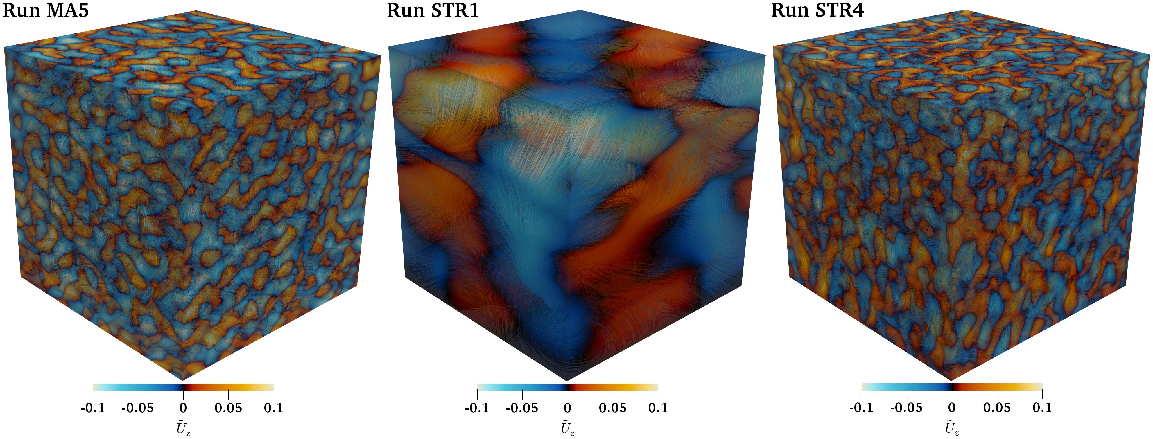
Figure 1: Vertical velocity $U_{z}$ near the periphery of the domain and streamlines of the flow from Runs MA5 (left), STR1 (middle), and STR4 (right).

3 Results

Three sets of simulations were made to study the effects of small-scale magnetic fields (Set SSD, Table 1), Mach number (Set MA, Table 2), and density stratification (Set STR, Table 3). In Sets SSD and MA the system is homogeneous and anisotropically forced while in Set STR the forcing is isotropic and a strong density stratification is present. Visualizations of typical flow patterns for three representative runs are shown in Figure 1. A somewhat surprising result is that the presence of strong density stratification is not clearly visible from the flow patterns, compare the left and right panels of Figure 1.

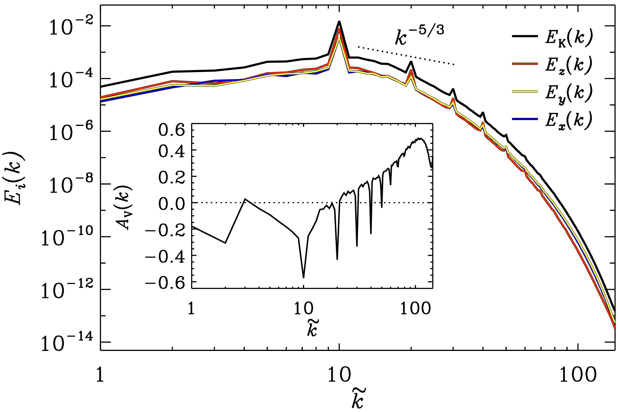
Figure 2: Power spectra of the total velocity (black), and its $x$ (blue), $y$ (yellow), and $z$ (red) components. The inset show the spectral anisotropy parameter $A_{\rm V}(k)$ according to Eq. (27) for Run MA7.

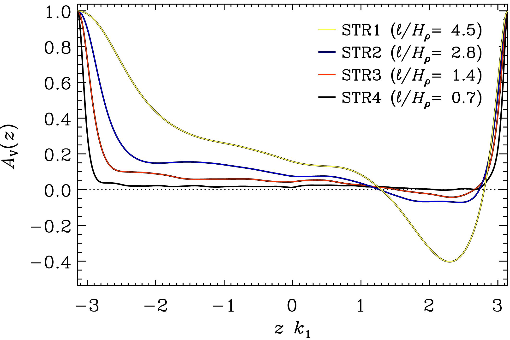
Figure 3: Anisotropy parameter $A_{\rm V}(z)$ from the runs in Set STR with varying $\tilde{k}_{\rm f}$.

3.1 Anisotropy of turbulence

Figure 2 shows the power spectra of the velocity from Run MA7. The power peaks near the forcing wavenumber for the total and vertical velocity. The peaks at the overtones of the forcing wavenumber arise because in the anisotropic case the forcing is no longer solenoidal. The spectrum is clearly steeper than the Kolmogorov (1941) (hereafter K41) $-5/3$ prediction. This is most likely due to the insufficient scale separation between the forcing and viscous scales which does not allow the formation of an inertial range. Indeed, even the highest resolution simulations up to date with $8192^{3}$ grid resolution are able recover only a rather modest well-defined inertial range (Iyer et al. 2017). The viscous scale is now well resolved due to the relatively modest Reynolds number (${\rm Re}\approx 15$) in the current simulations. It is also evident that the turbulence is anisotropic at all scales all the way down to the grid scale, see the red, blue and yellow curves in Figure 2. This is quantified by a spectral analogy of the anisotropy parameter:

$$A_{\rm V}(k)=\frac{E_{x}(k)+E_{y}(k)-2E_{z}(k)}{E_{\rm K}(k)},$$ (27)

where $E_{\rm K}(k)$ is the power spectrum of the total velocity and $E_{i}(k)$ are the power spectra of the individual velocity components. A representative result for $A_{\rm V}(k)$ is shown in the inset of Figure 2 for Run MA7. $A_{\rm V}(k)$ has a minimum at $k=k_{\rm f}$ which is due to the fact that the forcing mainly puts energy in the $z$ component of the velocity in this case.

While $A_{\rm V}(k)$ is mostly negative for large scales, it gradually increases and peaks around $0.5$ for $\tilde{k}\approx 100$. The fact that the anisotropy survives to the smallest resolved scales is in apparent disagreement with one of the cornerstones of the K41 theory which assumes that the turbulence is fully isotropic at small enough scales. However, the current simulations operate in a very modest Reynolds number regime which cannot be directly compared with the K41 theory which formally applies to fully developed turbulence at very high ${\rm Re}$.

In addition to using explicitly anisotropic forcing, setups where anisotropy arises naturally due to gravity and density stratification are studied in Set STR. By virtue of the isothermal equation of state this setup is characterised by a constant density scale height $H_{\rho}=c_{\rm s}^{2}/g=9/10$ such that simulation domain contains seven scale heights and a density contrast $\Delta\rho$ of more than a thousand. Although a modest resolution of 288 grid points was used, each scale height is covered by more than 40 grid points. This differs from the case of convection where the density (and pressure) scale height varies strongly as a function of depth and imposes much more restrictive constraints on the grid size (see, e.g. Käpylä et al. 2016).

Similar setups, albeit with somewhat lower stratification, were used in an earlier study by Brandenburg et al. (2012). They showed that turbulence anisotropy remains small when isotropic forcing is used unless the forcing scale is larger than the density scale height. This is confirmed by the current simulations where the scale separation ratio, quantified by the ratio of the forcing and system scales $\tilde{k}_{\rm f}=k_{\rm f}/k_{1}$, is varied between 1.5 and 10, see Figure 3 and Table 3 where a $z$-dependent variant of Equation (17) has been used. The density stratification-induced anisotropy is almost non-existent in the bulk of the domain in the case of the largest scale separation $\tilde{k}_{\rm f}=10$ or $\ell/H_{\rho}=0.7$. The stress-free and impenetrable boundary conditions enforce $U_{z}=0$ and lead to $A_{\rm V}=1$ at the vertical boundaries. In the cases with poorer scale separation or larger $\ell/H_{\rho}$, $A_{\rm V}$ tends to become more positive in the deep parts and obtains negative values near the surface. For the poorest scale separation (Run STR1, $\ell/H_{\rho}=4.5$) the magnitude of the anisotropy is comparable to typical values achieved with anisotropic forcing in Sets SSD and MA.

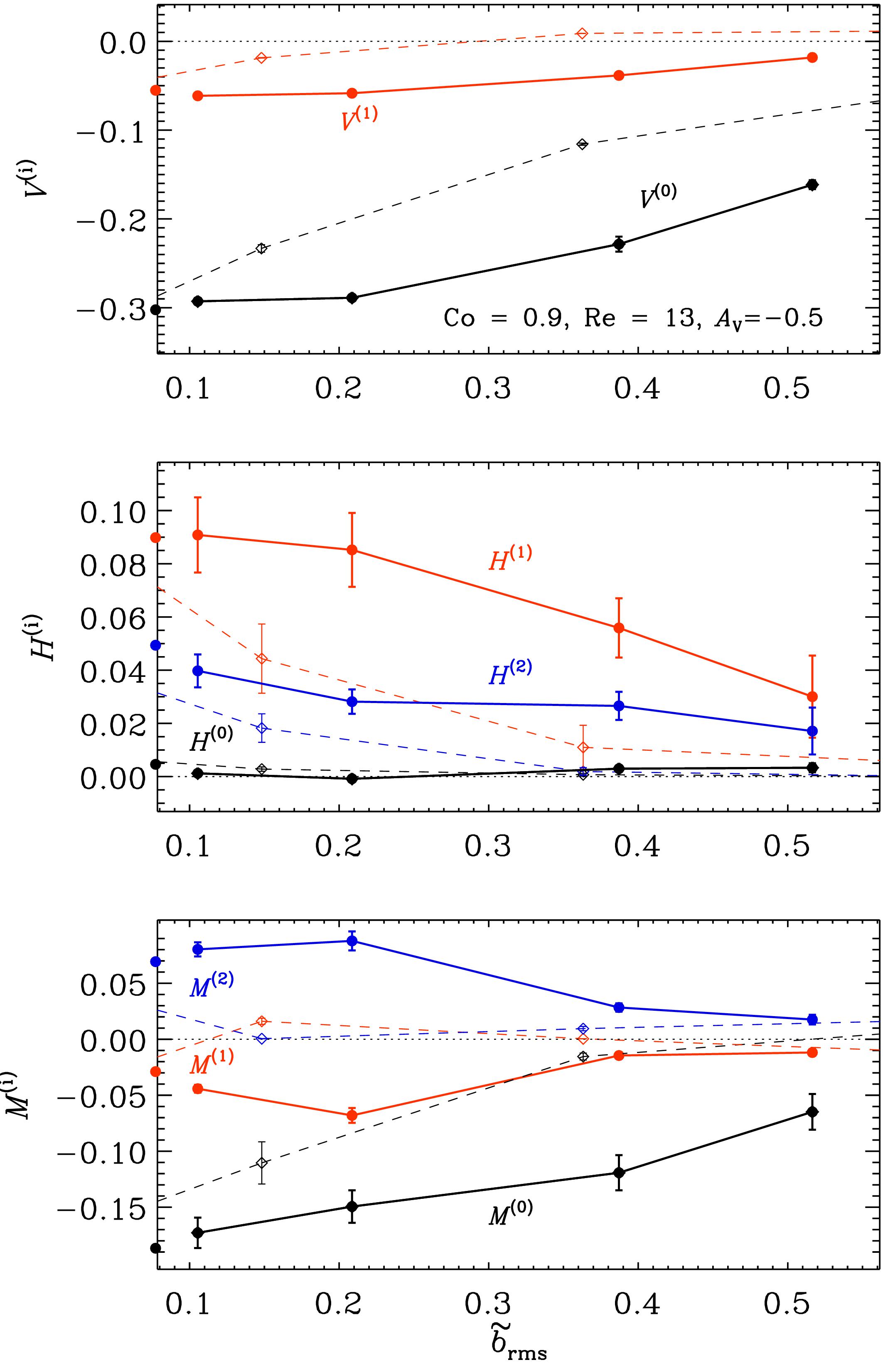
Figure 4: Coefficients $V^{(i)}$ (top), $H^{(i)}$ (middle), and $M^{(i)}$ (bottom) as functions of the normalized magnetic field strength $\tilde{b}_{\rm rms}=B_{\rm rms}/B_{\rm eq}$ from Sets SSD1-4. The thin dashed lines show the corresponding quantities from runs with an imposed vertical field from Käpylä (2019).

3.2 $\Lambda$ effect

3.2.1 Small-scale magnetic fields

Testing the dependence of purely small-scale magnetic fields is possible with the current homogeneous setups in cases where the magnetic Reynolds number exceeds that of the critical value for the excitation of a small-scale dynamo. Due to the absence of inhomogeneities, large-scale shear or helicity, no large-scale magnetic fields are expected to develop. A limited range of magnetic field strengths has been studied in the Set SSD, see Table 1. Run SSD1 with ${\rm Re}_{\rm M}=27$ corresponds to a slightly supercritical case whereas Run SSD4 corresponds to the highest ${\rm Re}_{\rm M}$ ($\approx 135$) that can be resolved with the adopted grid resolution. The saturation level $\tilde{b}_{\rm rms}=B_{\rm rms}/B_{\rm eq}$, where $B_{\rm rms}$ is the rms-value of the magnetic field, increases from roughly 10 to 50 per cent of the equipartition value in this range. In practice the characteristics of the flow, that is the Reynolds and Coriolis numbers and the degree of anisotropy, were kept fixed in all runs by adjusting $f_{0}$ and $f_{1}$ while ${\rm Re}_{\rm M}$ was varied by changing ${\rm Pm}$.

The results for the $\Lambda$ coefficients corresponding to Equations (24) to (26) from Sets SSD1-4 are shown in Figure 4. All of the coefficients are quenched as the small-scale magnetic fields increase: the values for $\tilde{b}_{\rm rms}\approx 0.5$ are typically roughly half of their hydrodynamic values. It is also evident that the quenching as a function of pure small-scale fields is weaker than that in the cases where an imposed large-scale vertical field is present, see the dashed lines in Figure 4 for the corresponding data from Käpylä (2019).

3.2.2 Dependence on Mach number

Although the Mach numbers in the foregoing studies (Käpylä & Brandenburg 2008; Käpylä 2019) were typically relatively low ($\mathcal{O}(0.1)$), it cannot be ruled out that a contribution due to compressibility is present. Furthermore, results from low-Reynolds number shear flows (Rogachevskii et al. 2011) suggest that compressibility significantly affects turbulent pumping for ${\rm Ma}\gtrsim 0.1$.

Results for the Mach number dependence from Set MA where $\Omega^{\star}=0.8$, $A_{\rm V}=-0.4$, and ${\rm Re}=15$ are kept fixed are shown in Figure 5. The range of Mach numbers spans from $0.015$ to $0.8$. Only the vertical stress $Q_{yz}$ for ${\rm Ma}\approx 0.8$ is statistically significantly different from the values obtained for lower ${\rm Ma}$ and even there the change is only on the order of ten per cent. Temporal fluctuations of $Q_{xz}$ increase, manifested by the drastically increased error estimates, as a function of ${\rm Ma}$ but the time-averaged values for all runs are still consistent with a ${\rm Ma}$-independent value.

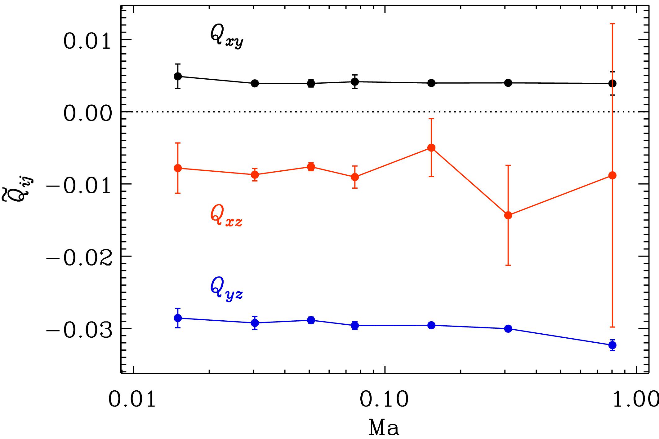
Figure 5: Off-diagonal Reynolds stresses $Q_{xy}$ (black), $Q_{xz}$ (red), and $Q_{yz}$ (blue) as functions of Mach number from Set MA, see Table 2.

3.2.3 Dependence on density stratification

In the foregoing analysis the $\Lambda$ effect resulted from the forcing that was designed to be anisotropic. While this is the case also in natural convection, a background density stratification also leads to anisotropy and should hence support a $\Lambda$ effect. This is indeed predicted by analytic theories (e.g. Kitchatinov & Rüdiger 2005; Pipin & Kosovichev 2018). Here this scenario is tested with a density-stratified setup with isotropic forcing in the Set STR, see Table 3.

The simulations considered here have $\Omega^{\star}\approx 0.8$ which is close to the Coriolis number where the Reynolds stresses obtain a maximum in Käpylä (2019). Furthermore, the simulation domain is situated at the equator at $\theta=90\degr$ where only the vertical Reynolds stress $Q_{yz}$ is non-zero. In order to isolate the contribution relevant for the $\Lambda$ effect, the horizontally averaged horizontal mean flows $\overline{U}_{x}$ and $\overline{U}_{y}$ are artificially removed from the solution similarly as in Rüdiger et al. (2019).

The results for the vertical stress $Q_{yz}$ are shown in Figure 6. The stress is positive everywhere even in the near-surface regions where $A_{\rm V}<0$. The results indicate that the scale separation ratio can play an important role for the density-induced anisotropy and consequently for the associated $\Lambda$ effect: both are substantial in the case of large-scale forcing and tend to approach zero when $\tilde{k}_{\rm f}$ increases. The values of $Q_{yz}$ are of the order of a few per cent of $u_{\rm rms}^{2}$ for $\ell/H_{\rho}=4.5$ whereas for $\ell/H_{\rho}=0.7$ the effect is no longer statistically significant at the equator. Figure 7(a) shows the normalized vertical stress $\tilde{Q}_{yz}$ from seven latitudes for the STR4 runs. The maximal values are generally on the order of one to two per cent of the squared rms-velocity. In this set the maximum value is obtained at $\theta=45\degr$ and only very small values are obtained at the equator ($\theta=90\degr$), see Figure 7(b). This, however, depends on the scale separation ratio because for a corresponding set with $\ell/H_{\rho}=4.5$, $Q_{yz}$ is consistent with a monotonic increase toward the equator. In all of these runs the sign of $A_{\rm V}$ differs from the sign of $Q_{yz}$. The mismatch of the signs of $Q_{yz}$ and $A_{\rm V}$ also suggests that non-locality may play a significant role when the scale separation ratio is small.

Another contribution to the $\Lambda$ effect due to a vertical gradient of the Coriolis number was discussed recently by Pipin & Kosovichev (2018). However, this effect is relevant only for large Coriolis numbers and thus not applicable here. Furthermore, the local Coriolis number ${\rm Co}=2\Omega_{0}\ell/u_{\rm rms}(z)$ varies by a factor between two and three in the current simulations (see the sixth column of Table 3) which is mild in comparison to the variation of four orders of magnitude in the solar convection zone as considered by Pipin & Kosovichev (2018).

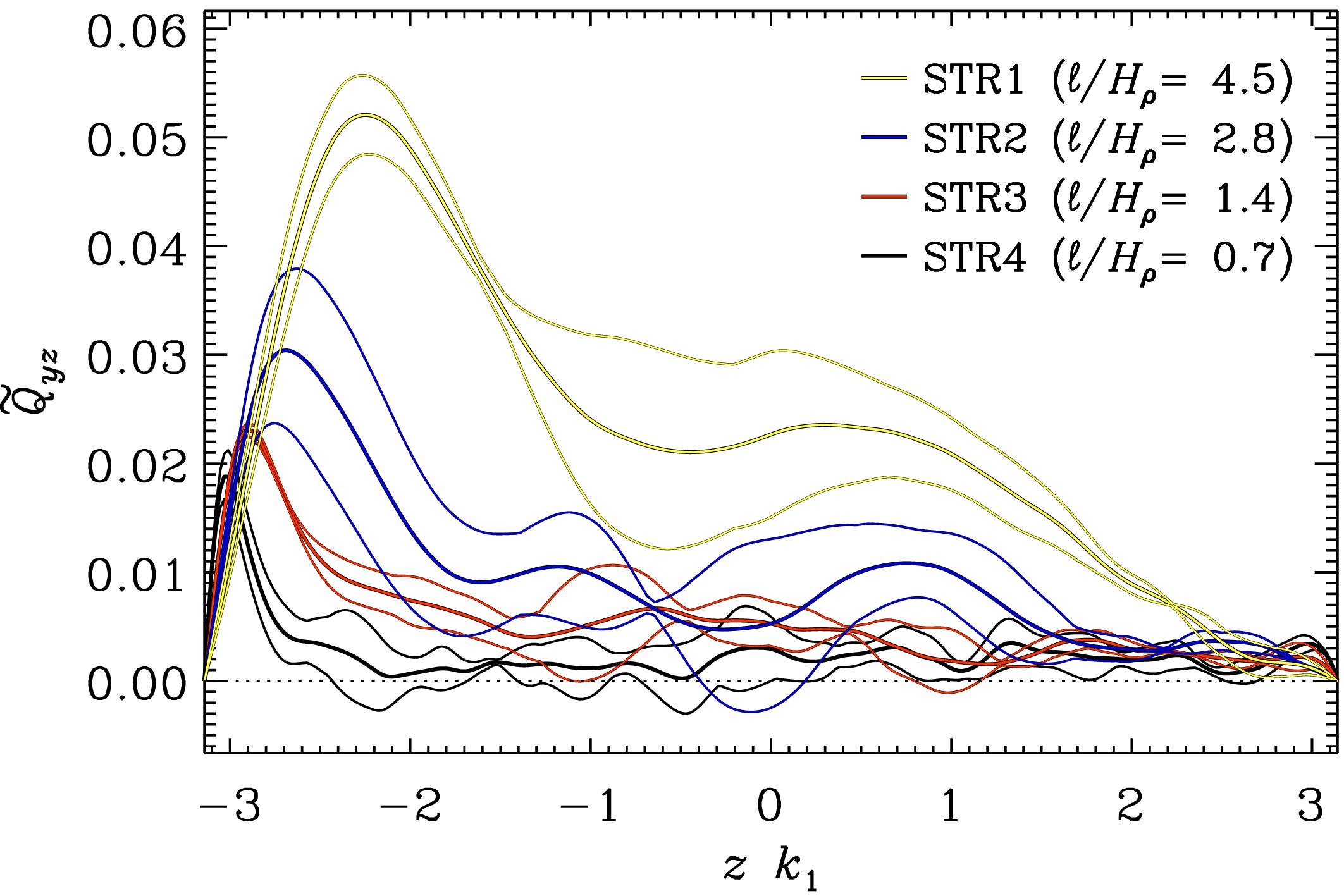
Figure 6: Vertical Reynolds stress $Q_{yz}$ normalized by the squared rms-velocity $u_{\rm rms}^{2}(z)$ in density-stratified runs with varying $\ell/H_{\rho}$.

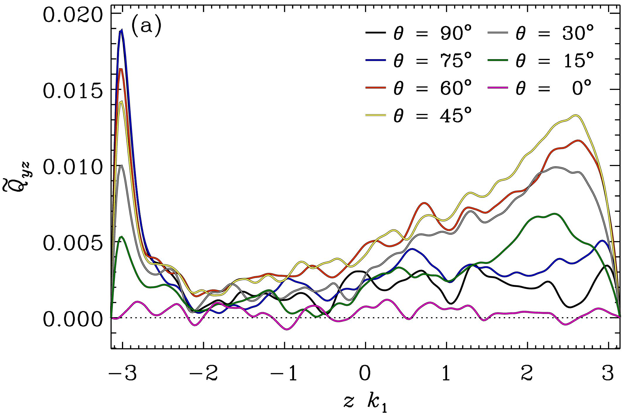
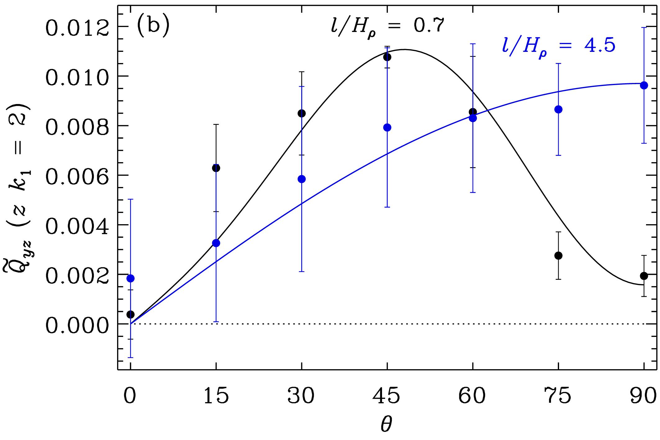
Figure 7: (a) Normalized vertical Reynolds stress $Q_{yz}$ as a function of height from runs with $\ell/H_{\rho}=0.7$ and $\Omega^{\star}=0.8$ from different colatitudes as indicated by the legend. (b) $\tilde{Q}_{yz}$ from $z\ k_{1}=2$ as functions of $\theta$ from two sets with $\ell/H_{\rho}=0.7$ (black) and $\ell/H_{\rho}=4.5$ (blue). The curves show best fits according to Eq. (25) with $V^{(0)}=0.011$, $V^{(1)}=0.027$, $V^{(2)}=-0.036$ for $\ell/H_{\rho}=0.7$ and $V^{(0)}=0.010$ for $\ell/H_{\rho}=4.5$

4 Conclusions

The effects of small-scale magnetic fields, compressibility and background density stratification on the $\Lambda$ effect were studied with numerical simulations of forced turbulence with an isothermal equation of state.

The small-scale magnetic fields generated by a small-scale dynamo lead to a significantly milder quenching of the $\Lambda$ effect in comparison to cases where also a uniform large-scale field is imposed (see, e.g. Käpylä 2019). Thus is appears that the small-scale dynamo alone could not explain the severely quenched differential rotation in recent semi-global convection simulations (Käpylä et al. 2017). It is also conceivable that other MHD instabilities, such as the magnetorotational instability (e.g. Masada 2011), can be excited in the high-resolution convection simulations, leading to repercussions for differential rotation.

Another aspect that has hitherto received little attention is the Mach number dependence of the $\Lambda$ effect although most numerical studies of the subject operate in a fully compressible regime (e.g. Käpylä & Brandenburg 2008; Käpylä 2019). The current results indicate that while the fluctuations of the $\Lambda$ coefficients tend to increase with ${\rm Ma}$, the mean values are consistent with a ${\rm Ma}$-independent value at least until ${\rm Ma}\approx 0.8$. Thus the effects of compressibility have most likely not had a significant contribution to the results regarding the $\Lambda$ effect in the previous numerical studies.

In the mean-field-theoretical treatment the $\Lambda$ effect has distinct contributions from the anisotropy of turbulence and from background density stratification. The former has been modeled by an anisotropic forcing in homogeneous and fully periodic setups (e.g. Käpylä 2019) while the latter requires a mean density gradient and inevitably leads to inhomogeneity. The latter setup was studied with a set of strongly stratified simulations where turbulence was driven by isotropic forcing. Thus the anisotropy of the turbulence was induced by the density stratification. The current results indicate that the anisotropy is weak in cases where the forcing scale is smaller or comparable with the density scale height. The vertical velocities are suppressed (enhanced) over the horizontal components in the deep (near-surface) parts of the simulations. The vertical Reynolds stress and hence the $\Lambda$ effect are, however, positive everywhere.

These results suggest an opposite sign of the vertical $\Lambda$ effect due to the density gradient in comparison to contribution from the vertically dominated homogeneous turbulence at a comparable Coriolis number. Further studies involving more realistic flows (e.g. convection) are needed to study the relevance of these findings for solar and stellar differential rotation.