Coresets for Ordered Weighted Clustering

Abstract

We design coresets for Ordered $k$-Median, a generalization of classical clustering problems such as $k$-Median and $k$-Center, that offers a more flexible data analysis, like easily combining multiple objectives (e.g., to increase fairness or for Pareto optimization). Its objective function is defined via the Ordered Weighted Averaging (OWA) paradigm of Yager (1988), where data points are weighted according to a predefined weight vector, but in order of their contribution to the objective (distance from the centers).

A powerful data-reduction technique, called a coreset, is to summarize a point set $X$ in $\mathbb{R}^{d}$ into a small (weighted) point set $X^{\prime}$, such that for every set of $k$ potential centers, the objective value of the coreset $X^{\prime}$ approximates that of $X$ within factor $1\pm\epsilon$. When there are multiple objectives (weights), the above standard coreset might have limited usefulness, whereas in a simultaneous coreset, which was introduced recently by Bachem and Lucic and Lattanzi (2018), the above approximation holds for all weights (in addition to all centers). Our main result is a construction of a simultaneous coreset of size $O_{\epsilon,d}(k^{2}\log^{2}|X|)$ for Ordered $k$-Median.

To validate the efficacy of our coreset construction we ran experiments on a real geographical data set. We find that our algorithm produces a small coreset, which translates to a massive speedup of clustering computations, while maintaining high accuracy for a range of weights.

1 Introduction

We study data reduction (namely, coresets) for a class of clustering problems, called ordered weighted clustering, which generalizes the classical $k$-Center and $k$-Median problems. In these clustering problems, the objective function is computed by ordering the $n$ data points by their distance to their closest center, then taking a weighted sum of these distances, using predefined weights $v_{1}\geq\cdots\geq v_{n}\geq 0$. These clustering problems can interpolate between $k$-Center (the special case where $v_{1}=1$ is the only non-zero weight) and $k$-Median (unit weights $v_{i}=1$ for all $i$), and therefore offer flexibility in prioritizing points with large service cost, which may be important for applications like Pareto (multi-objective) optimization and fair clustering. In general, fairness in machine learning is seeing a surge in interest, and is well-known to have many facets. In the context of clustering, previous work such as the fairlets approach of  [CKLV17], has addressed protected classes, which must be identified in advance. In contrast, ordered weighted clustering addresses fairness towards remote points (which can be underprivileged communities), without specifying them in advance. This is starkly different from many application domains, where remote points are considered as outliers (to be ignored) or anomalies (to be detected), see e.g., the well-known survey by  [CBK09].

Formally, we study two clustering problems in Euclidean space $\mathbb{R}^{d}$. In both of them, the input is $n$ data points $X\subset\mathbb{R}^{d}$ (and $k\in[n]$), and the goal is to find $k$ centers $C\subset\mathbb{R}^{d}$ that minimize a certain objective $\operatorname{cost}(X,C)$. In Ordered $k$-Median, there is a predefined non-decreasing weight vector $v\in\mathbb{R}_{+}^{n}$, and the data points $X=\{x_{1},\ldots,x_{n}\}$ are ordered by their distance to the centers, i.e., $d(x_{1},C)\geq\cdots\geq d(x_{n},C)$, to define the objective

$$\operatorname{cost}_{v}(X,C):=\sum_{i=1}^{n}v_{i}\cdot d(x_{i},C),$$ (1)

where throughout $d(\cdot,\cdot)$ refers to $\ell_{2}$ distance, extended to sets by the usual convention $\mathsf{dist}(x,C):=\min_{c\in C}\mathsf{dist}(x,c)$. This objective follows the Ordered Weighted Averaging (OWA) paradigm of  [Yag88], in which data points are weighted according to a predefined weight vector, but in order of their contribution to the objective. The $p$-Centrum problem is the special case where the first $p$ weights equal $1$ and the rest are $0$, denoting its objective function by $\operatorname{cost}_{p}(X,C)$. Observe that this problem already includes both $k$-Center (as $p=1$) and $k$-Median (as $p=n$).

A powerful data-reduction technique, called a coreset, is to summarize a large point set $X$ into a (small) multiset $X^{\prime}$, that approximates well a given cost function (our clustering objective) for every possible candidate solution (set of centers). More formally, $X^{\prime}$ is an $\epsilon$-coreset of $X$ for clustering objective $\operatorname{cost}(\cdot,\cdot)$ if it approximates the objective within factor $1\pm\epsilon$, i.e.,

$$\forall C\subset\mathbb{R}^{d},|C|=k,\quad\operatorname{cost}(X^{\prime},C)\in(1\pm\epsilon)\operatorname{cost}(X,C).$$

The size of $X^{\prime}$ is the number of distinct points in it. The above notion, sometimes called a strong coreset, was proposed by  [HM04], following a weaker notion of  [AHPV04]. In recent years it has found many applications, see the surveys of  [AHV05],  [Phi16] and  [MS18], and references therein.

The above coreset definition readily applies to ordered weighted clustering. However, a standard coreset is constructed for a specific clustering objective, i.e., a single weight vector $v\in\mathbb{R}_{+}^{n}$, which might limit its usefulness. The notion of a simultaneous coreset, introduced recently by  [BLL18], requires that all clustering objectives are preserved, i.e., the $(1+\epsilon)$-approximation holds for all weight vectors in addition to all centers. This “simultaneous” feature is valuable in data analysis, since the desired weight vector might be application and/or data dependent, and thus not known when the data reduction is applied. Moreover, since ordered weighted clustering includes classical clustering, e.g., $k$-Median and $k$-Center as special cases, all these different analyses may be performed on a single simultaneous coreset.

1.1 Our Contribution

Our main result is (informally) stated as follows. To simplify some expressions, we use $O_{\epsilon,d}(\cdot)$ to suppress factors depending only on $\epsilon$ and $d$. The precise dependence appears in the technical sections.

Theorem 1.1 (informal version of Theorem 4.6).

There exists an algorithm that, given an $n$-point data set $X\subset\mathbb{R}^{d}$ and $k\in[n]$, computes a simultaneous $\epsilon$-coreset of size $O_{\epsilon,d}(k^{2}\log^{2}{n})$ for Ordered $k$-Median.

Our main result is built on top of a coreset result for $p$-Centrum (the special case of Ordered $k$-Median in which the weight vector is $1$ in the first $p$ components and $0$ in the rest). For this special case, we have an improved size bound, that avoids the $O(\log^{2}n)$ factor, stated as follows. Note that this coreset is for a single value of $p$ (and not simultaneous).

Theorem 1.2 (informal version of Theorem 4.4).

There exists an algorithm that, given an $n$-point data set $X\subset\mathbb{R}^{d}$ and $k,p\in[n]$, computes an $\epsilon$-coreset of size $O_{\epsilon,d}(k^{2})$ for $p$-Centrum.

The size bounds in the two theorems are nearly tight. The dependence on $n$ in Theorem 1.1 is unavoidable, because we can show that the coreset size has to be $\Omega(\log n)$, even when $k=d=1$ (see Theorem 4.9). For both Theorem 1.1 and Theorem 1.2, the hidden dependence on $\epsilon$ and $d$ is $(\frac{1}{\epsilon})^{d+O(1)}$. This factor matches known lower bounds [D. Feldman, private communication] and state-of-the-art constructions of coresets for $k$-Center (which is a special case of Ordered $k$-Median) [AP02].

A main novelty of our coreset is that it preserves the objective for all weights ($v\in\mathbb{R}_{+}^{n}$ in the objective function) simultaneously. It is usually easy to combine coresets for two data sets, but in general it is not possible to combine coresets for two different objectives. Moreover, even if we manage to combine coresets for two objectives, it is still nontrivial to achieve a small coreset size for infinitely many objectives (all possible weight vectors $v\in\mathbb{R}_{+}^{n}$). See the overview in Section 1.2 for more details on the new technical ideas needed to overcome these obstacles.

We evaluate our algorithm on a real 2-dimensional geographical data set with about 1.5 million points. We experiment with the different parameters for coresets of $p$-Centrum, and we find out that the empirical error is always far lower than our error guarantee $\epsilon$. As expected, the coreset is much smaller than the input data set, leading to a massive speedup (more than 500 times) in the running time of computing the objective function. Perhaps the most surprising finding is that a single $p$-Centrum coreset (for one “typical” $p$) empirically serves as a simultaneous coreset, which avoids the more complicated construction and the dependence on $n$ in Theorem 1.1, with a coreset whose size is only 1% of the data set. Overall, the experiments confirm that our coreset is practically efficient, and moreover it is suitable for data exploration, where different weight parameters are needed.

1.2 Overview of Techniques

We start with discussing Theorem 1.2 (which is a building block for Theorem 1.1). Its proof is inspired by  [HK07], who constructed coresets for $k$-Median clustering in $\mathbb{R}^{d}$ by reducing the problem to its one-dimensional case. We can apply a similar reduction, but the one-dimensional case of $p$-Centrum is significantly different from $k$-Median. One fundamental difference is that the objective counts only the $p$ largest distances, hence the subset of “contributing” points depends on the center. We deal with this issue by introducing a new bucketing scheme and a charging argument that relates the error to the $p$ largest distances. See Section 3 for more details.

The technical difficulty in Theorem 1.1 is two-fold: how to combine coresets for two different weight vectors, and how to handle infinitely many weight vectors. The key observation is that every Ordered $k$-Median objective can be represented as a linear combination of $p$-Centrum objectives (see Lemma 4.7). Thus, it suffices to compute a simultaneous coreset for $p$-Centrum for all $p\in[n]$. We achieve this by “combining” the individual coresets for all $p\in[n]$, while crucially utilizing the special structure of our construction of a $p$-Centrum coreset, but unfortunately losing an $O(\log n)$ factor in the coreset size. In the end, we need to “combine” the $n$ coresets for all $p\in[n]$, but we can avoid losing an $O(n)$ factor by discretizing the values of $p$, so that only $O(\log n)$ coresets are combined, The result is a simultaneous coreset of size $O_{\epsilon,d}(\log^{2}n)$, see Section 4 for more details.

1.3 Related Work

The problem of constructing strong coresets for $k$-Means, $k$-Median, and other objectives has received significant attention from the research community [FMSW10, FL11, LS10, BHPI02, Che09]. For example,  [HM04] designed the first strong coreset for $k$-Means.  [FSS13] provided coresets for $k$-Means, PCA and projective clustering that are independent of the dimension. Recently,  [SW18] generalized the results of  [FSS13] and obtained strong coresets for $k$-Median and for subspace approximation that are independent of the dimension $d$.

Ordered $k$-Median and its special case $p$-Centrum generalize $k$-Center and are thus APX-hard even in $\mathbb{R}^{2}$ [MS84]. However, $p$-Centrum may be solved optimally in polynomial time for special cases such as lines and trees [Tam01]. The first provable approximation algorithm for Ordered $k$-Median was proposed by  [AS18], and they gave $2$-approximation for trees and $O(\log n)$-approximation for general metrics. The approximation ratio for general metrics was drastically improved to $38$ by  [BSS18], improved to $18+\epsilon$ by  [CS18b], and finally a $(5+\epsilon)$-approximation was obtained very recently by  [CS18a].

Previous work on fairness in clustering has followed the disparate impact doctrine of  [FFM⁺15], and addressed fairness with respect to protected classes, where each cluster in the solution should fairly represent every class.  [CKLV17] have designed approximation algorithms for $k$-Center and $k$-Median, and their results were refined and extended by  [RS18] and  [BCN19]. Recent work by  [SSS18] designs coresets for fair $k$-Means clustering. However, these results are not applicable to ordered weighted clustering.

2 Preliminaries

Throughout this paper we use capital letters other than $I$ and $J$ to denote finite subsets of $\mathbb{R}^{d}$. We recall some basic terminology from [HK07]. For a set $Y\subset\mathbb{R}$, define its mean point to be

$$\mu(Y):=\frac{1}{|Y|}\sum_{y\in Y}y,$$ (2)

and its cumulative error to be

$$\delta(Y):=\sum_{y\in Y}|y-\mu(Y)|.$$ (3)

Let $I(Y):=[\inf Y,\sup Y]$ denote the smallest closed interval containing $Y$. The following facts from [HK07] will be useful in our analysis.

Lemma 2.1.

For every $Y\subset\mathbb{R}$ and $z\in\mathbb{R}$,

• $\sum_{y\in Y}\Big{|}|z-y|-|z-\mu(Y)|\Big{|}\leq\delta(Y)$; and

• if $z\notin I(Y)$ then $\sum_{y\in Y}|y-z|=|Y|\cdot|\mu(Y)-z|$.

It will be technically more convenient to treat a coreset as a point set $X^{\prime}\subset\mathbb{R}^{d}$ associated with integer weights $w:X^{\prime}\to\mathbb{N}$, which is equivalent to a multiset (with weights representing multiplicity), and thus the notation of $\operatorname{cost}_{v}(X^{\prime},C)$ in (1) is well-defined. (These weights $w$ are unrelated to the predefined weights $\{v_{i}\}$.) While our algorithm always produces $X^{\prime}$ with integral weights $w$, our proof requires fractional weights during the analysis, and thus we extend (2) and (3) to a point set $Y$ with weights $w:Y\rightarrow\mathbb{R}_{+}$ by defining

$$\mu_{w}(Y) :=\frac{1}{\sum_{y\in Y}{w(y)}}\sum_{y\in Y}{w(y)\cdot y},$$

$$\delta_{w}(Y) :=\sum_{y\in Y}{w(y)\cdot|y-\mu(Y)|}.$$

We will use the fact that in one-dimensional Euclidean space, $p$-Centrum can be solved (exactly) in polynomial time by dynamic programming, as shown by  [Tam01].

Lemma 2.2 ([Tam01]).

There is a polynomial-time algoritm that, given a set of one-dimensional points $X=\{x_{1},\ldots,x_{n}\}\subset\mathbb{R}$ and parameters $k,p\in[n]$, computes a set of $k$ centers $C\subset\mathbb{R}^{d}$ that minimizes $\operatorname{cost}_{p}(X,C)$.

3 The Basic Case: $p$-Centrum for $k=d=1$ (one facility in one-dimensional data)

In this section we illustrate our main ideas by constructing a coreset for $p$-Centrum in the special case of one facility in one-dimensional Euclidean space (i.e., $k=d=1$). This is not a simultaneous coreset, but rather for a single $p$. The key steps of our construction described below will be repeated, with additional technical complications, also in the general case of $p$-Centrum, i.e., $k$ facilities in dimension $d$.

We will need two technical lemmas, whose proofs appear in Section 3.1. The first lemma bounds $\delta(Y)$ by the cost of connecting $Y$ to an arbitrary point outside $I(Y)$ (which in turn is part of the objective in certain circumstances).

Lemma 3.1.

Let $Y\subset\mathbb{R}$ be a set with (possibly fractional) weights $w:Y\to\mathbb{R}_{+}$. Then for every $z\in\mathbb{R}$ such that $z\not\in I(Y)$ or $z$ is an endpoint of $I(Y)$,

$$\delta_{w}(Y)\leq 2\sum_{y\in Y}w(y)\cdot|y-z|.$$

Recall that $k=1$, hence the cost in an instance of $p$-Centrum is the sum of the $p$ largest distances to the center. In the analysis of our coreset it will be useful to replace some points of the input set $X$ with another set $Y$. The second lemma will be used to bound the resulting increase in the cost; it considers two sequences, denoted $X$ and $Y$, of the connection costs, and bounds the difference between the sum of the $p$ largest values in $X$ and that in $Y$ by a combination of $\ell_{\infty}$ and $\ell_{1}$ norms.

Lemma 3.2.

Let $X=(x_{1},\ldots,x_{n})$ and $Y=(y_{1},\ldots,y_{n})$ be two sequences of real numbers. Then for all $S\subseteq[n]$,

$$|\operatorname{top}_{p}(X)-\operatorname{top}_{p}(Y)|\leq p\max_{i\in S}|x_{i}-y_{i}|+\sum_{i\in[n]\setminus S}|x_{i}-y_{i}|,$$

where $\operatorname{top}_{p}(Z)$ is the sum of the $p$ largest numbers in $Z$.

Outline of the Coreset Construction

In the context of a one-dimensional point set $X\subset\mathbb{R}$, the term interval will mean a subset of $X$ that spans a contiguous subsequence under a fixed ordering of the points, i.e., a subset $\{x_{i},\ldots,x_{j}\}$ when the points in $X$ are ordered as $x_{1}\leq\ldots\leq x_{n}$. Informally, our coreset construction works as follows. First, use Lemma 2.2 to find an optimal center $y^{*}$, its corresponding optimal cost $\mathrm{OPT}$, and a subset $P\subset X$ of size $|P|=p$ that contributes to the optimal cost. Then partition the data into three intervals, namely $X=L\cup R\cup Q$, as follows. Points from $P$ that are smaller or equal to $y^{*}$ are placed in $L$, points from $P$ that are larger than $y^{*}$ are placed in $R$, and all other points are placed in $Q=X\setminus P$. Now split $L$, $Q$ and $R$ into sub-intervals, in a greedy manner that we describe below, and represent the data points in each sub-interval by adding to the coreset a single point, whose weight is equal to the number of data points it replaces. See Figure 1 for illustration.

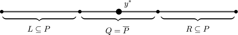
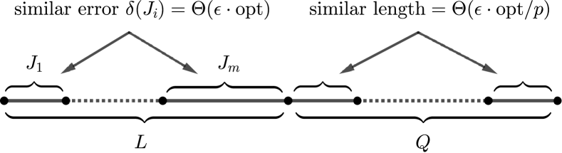
Figure 1: Coreset construction for $p$-Centrum with $k=1$ facilities in dimension $d=1$. The left figure depicts the partition of the data into $X=(L\cup R)\cup Q$, where $P=L\cup R$ contains the $p$ furthest points from an optimal center $y^{*}$. The right figure shows the different manners of splitting $L$ and $Q$ into intervals.

To split $L$ into sub-intervals, scan its points from the smallest to the largest and pack them into the same sub-interval $J$ as long as their cumulative error $\delta(J)$ is below a threshold set to $\Theta({\varepsilon\cdot\mathrm{OPT}})$. This ensures, by Lemma 3.1, a lower bound on their total connection cost to the optimal center $y^{*}$, which we use to upper bound the number of such intervals (which immediately affects the size of the coreset) by $O\left({1\over\epsilon}\right)$. The split of $R$ is done similarly. To split $Q=X\setminus P$, observe that the distance from every $q\in Q$ to the center $y^{*}$ is less than $\frac{\mathrm{OPT}}{p}$, hence the diameter of $Q$ is less than $\frac{2\mathrm{OPT}}{p}$, and $Q$ can be partitioned into $O(\frac{1}{\varepsilon})$ sub-intervals of length $O(\frac{\varepsilon\mathrm{OPT}}{p})$. Observe that the construction for $Q$ differs from that of $L$ and $R$.

Let $D$ denote the coreset resulting from the above construction. To prove that the resulting coreset has the desired error bound for every potential center $y\in\mathbb{R}$, we define an intermediate set $Z$ that contains a mix of points from $X$ and $D$. We stress that $Z$ depends on the potential center $y\in\mathbb{R}$, which is possible because $Z$ is used only in the analysis. The desired error bound follows by bounding both $|\operatorname{cost}(Z,y)-\operatorname{cost}(X,y)|$ and $|\operatorname{cost}(Z,y)-\operatorname{cost}(D,y)|$, (here we use Lemma 3.2), and applying the triangle inequality.

Detailed Construction and Coreset Size

We now give a formal description of our coreset construction. Let $X=\{x_{1},\ldots,x_{n}\}\subset\mathbb{R}$ be the input data set, and recall that $\operatorname{cost}_{p}(X,y)$ for a point $y\in\mathbb{R}$ is the sum of the $p$ largest numbers in $\{|x_{1}-y|,\ldots,|x_{n}-y|\}$. Denote the optimal center by $y^{*}:=\mathrm{argmin}_{y\in\mathbb{R}}\operatorname{cost}_{p}(X,y)$, and the corresponding optimal cost by $\mathrm{OPT}:=\operatorname{cost}_{p}(X,y^{*})$. By Lemma 2.2, $y^{*}$ and $\mathrm{OPT}$ can be computed in polynomial time. Next, sort $X$ by distances to $y^{*}$. For simplicity, we shall assume the above notation for $X$ is already in this sorted order, i.e., $|x_{1}-y^{*}|\geq\cdots\geq|x_{n}-y^{*}|$. Thus, $\operatorname{cost}_{p}(X,y^{*})=\sum_{i=1}^{p}|x_{i}-y^{*}|$.

Let $P:=\{x_{1},\ldots,x_{p}\}$, $L:=\{x_{i}\leq y^{*}:x_{i}\in P\}$, $R:=\{x_{i}>y^{*}:x_{i}\in P\}$ and $Q:=X\setminus P$. By definition, $X$ is partitioned into $L$, $Q$ and $R$, which form three intervals located from left to right. We now wish to split $L$, $Q$ and $R$ into sub-intervals, and then we will add to $D$ the mean of the points in each sub-interval, with weight equal to the number of such points.

Split $L$ into sub-intervals from left to right greedily, such that the cumulative error of each interval $J$ does not exceed $\frac{2\varepsilon\cdot\mathrm{OPT}}{21}$, and each sub-intervals is maximal, i.e., the next point cannot be added to it. Split $R$ into sub-intervals similarly but from right to left. We need to bound the number of sub-intervals produced in this procedure.

For sake of analysis, we consider an alternative split of $L$ that is fractional, i.e., allows assigning a point fractionally to multiple sub-intervals, say $1/3$ to the sub-interval to its left and $2/3$ to the sub-interval to its right. The advantage of this fractional split is that all but the last sub-interval have cumulative error exactly $\frac{2\varepsilon\cdot\mathrm{OPT}}{21}$. We show in Lemma 3.3 that the number of sub-intervals produced in the original integral split is at most twice that of the fractional split, and thus it would suffice to bound the latter by $O(\frac{1}{\varepsilon})$.

Lemma 3.3.

The number of sub-intervals in the integral split is at most twice than that of the fractional split.

Proof.

It suffices to show that for every $t$, the first $2t$ sub-intervals produced by the integral partitioning contain at least as many points as the first $t$ sub-intervals produced by the fractional partitioning. For this, the key observation is that in a fractional split, only the two endpoints of a sub-interval may be fractional, because the cumulative error of a singleton set is $0$.

We prove the above by induction on $t$. The base case $t=1$ follows from these observations, since the fractional sub-interval may be broken into two integral sub-intervals, each with cumulative error at most $\frac{2\varepsilon\cdot\mathrm{OPT}}{21}$. Suppose the claim holds for $t-1$ and let us show that it holds for $t$. Since the cumulative error is monotone in adding new points, we may assume the first $t-1$ sub-intervals from fractional split contain as many points as the first $2(t-1)$ sub-intervals from integral split. Now similarly to the base case, the $t$-th fractional interval may be broken into two integral sub-intervals, and this proves the inductive step. ∎

To see that the number of sub-intervals produced by a fractional partitioning of $L$ is $O(\frac{1}{\varepsilon})$, we use Lemma 3.1. Suppose there are $m$ such sub-intervals $J_{1},...,J_{m}$. We can assume that the first $m-4$ of them do not contain $y^{*}$ and have cumulative error at least $\frac{2\varepsilon\cdot\mathrm{OPT}}{21}$, because at most two sub-intervals can contain $y^{*}$, and at most one sub-interval from each of $L$ and $R$ may have cumulative error less than $\frac{2\varepsilon\cdot\mathrm{OPT}}{21}$. By Lemma 3.1 and the fact that $y^{*}$ is not in the first $i\leq m-4$ sub-intervals,

$$\mathrm{OPT}\geq\sum_{i=1}^{m-4}\sum_{x:x\in J_{i}}|x-y^{*}|\geq\frac{1}{2}\sum_{i=1}^{m-4}\delta_{w}(J_{i})=(m-4)\frac{\varepsilon\cdot\mathrm{OPT}}{21}.$$

Thus $m=O(\frac{1}{\varepsilon})$, and by Lemma 3.3 a similar bound holds also for the number of sub-intervals in the integral split of $L$ and of $R$.

Now split $Q$ greedily into maximal sub-intervals of length not larger than $\frac{\varepsilon\cdot\mathrm{OPT}}{3p}$. Since $\max_{q\in Q}|q-y^{*}|\leq|x_{p}-y^{*}|\leq\frac{\mathrm{OPT}}{p}$, the length of $I(Q)$ is at most $\frac{2\mathrm{OPT}}{p}$, and we conclude that $Q$ is split into at most $\frac{3}{\varepsilon}+1$ sub-intervals.

Finally, construct the coreset $D$ from the sub-intervals, by adding to $D$ the mean of each sub-interval in $D$, with weight that is the number of points in this sub-interval. Since the total number of sub-intervals is $O(\frac{1}{\epsilon})$, the size of the coreset $D$ is also bounded by $O(\frac{1}{\epsilon})$.

Coreset Accuracy

To prove that $D$ is an $\epsilon$-coreset for $X$, fix a potential center $y\in\mathbb{R}$ and let us prove that $|\operatorname{cost}_{p}(D,y)-\operatorname{cost}_{p}(X,y)|\leq\varepsilon\cdot\mathrm{OPT}$, where we interpret $D$ as a multi-set. Let $P_{1}\subseteq X$ denote the set of $p$ points in $X$ that are farthest from $y$. Now define an auxiliary set $Z:=\{z_{1},\ldots,z_{n}\}$, as follows. For each $i\in[n]$, let $X_{i}\subset X$ be the sub-interval containing $x_{i}$ in the construction of the coreset (recall it uses the optimal center $y^{*}$ and not $y$), and let $\pi(x_{i})=\mu(X_{i})$ be its representative in the coreset $D$. Now if (a) $i\leq p$; (b) $y\not\in X_{i}$; and (c) $P_{1}\cap X_{i}$ is either empty or all of $X_{i}$; then let $z_{i}:=\pi(x_{i})$. Otherwise, let $z_{i}:=x_{i}$.

We now aim to bound $|\operatorname{cost}_{p}(Z,y)-\operatorname{cost}_{p}(D,y)|$ using Lemma 3.2 with $S=\{p+1,...,n\}$. Consider first some $i\in S$ (i.e., $i>p$). Then

$$|d(z_{i},y)-d(\pi(x_{i}),y)| \leq|z_{i}-\pi(x_{i})|$$

$$=|x_{i}-\pi(x_{i})|\leq\frac{\varepsilon\cdot\mathrm{OPT}}{3p}.$$ (4)

Consider next $i\notin S$ (i.e., $i\leq p$). We can have $z_{i}\neq\pi(x_{i})$ only if $y\in X_{i}$ or if $P_{1}\cap X_{i}$ is neither empty nor all of $X_{i}$. This can happen for at most $7$ distinct sub-intervals $X_{i}$, because the former case can happen for at most $3$ sub-intervals $X_{i}$ (by a simple case analysis of how many sub-intervals might have an endpoint at $y$, e.g., two from $L$, or one from each of $L,R,Q$) and because $P_{1}$ is contained in $2$ intervals (to the left and right of $y$), and each of them can intersect at most $2$ distinct sub-intervals $X_{i}$ without containing all of $X_{i}$. We obtain

$$\sum_{i=1}^{p} |d(z_{i},y)-d(\pi(x_{i}),y)|=$$

$$=\sum_{i\in[p]:z_{i}\neq\pi(x_{i})}|d(x_{i},y)-d(\pi(x_{i}),y)|$$ (5)

$$\leq\sum_{X_{i}:i\in[p],(y\in X_{i})\lor(P_{1}\cap X_{i}\neq\emptyset,X_{i})}\delta(X_{i})$$ (6)

$$\leq 7\cdot\frac{2\varepsilon\cdot\mathrm{OPT}}{21}=\frac{2\varepsilon\cdot\mathrm{OPT}}{3},$$ (7)

where (6) is by Lemma 2.1, and (7) is by the fact that these $X_{i}$ are from $L$ or $R$ (recall $i\leq p$) and thus have a bounded cumulative error.

Applying Lemma 3.2 to our $S=\{p+1,...,n\}$ together with (4) and (7), we obtain

$$|\operatorname{cost}_{p}(Z,y)-\operatorname{cost}_{p}(D,y)|\leq p\cdot\frac{\varepsilon\cdot\mathrm{OPT}}{3p}+\frac{2\varepsilon\cdot\mathrm{OPT}}{3}=\varepsilon\cdot\mathrm{OPT}.$$

Lastly, we need to prove that $\operatorname{cost}_{p}(Z,y)=\operatorname{cost}_{p}(X,y)$. We think of $Z$ as if it is obtained from $X$ by replacing each $x_{i}$ with its corresponding $z_{i}=\pi(x_{i})=\mu(X_{i})$. We can of course restrict attention to indices where $z_{i}\neq x_{i}$, which happens only if all three requirements (a)-(c) hold. Moreover, whenever this happens for point $x_{i}$, it must happen also for all points in the same sub-interval $X_{i}$, i.e., every $x_{j}\in X_{i}$ is replaced by $z_{j}=\pi(x_{j})=\mu(X_{i})$. By requirement (c), $X_{i}$ is either disjoint from $P_{1}$ or contained in $P_{1}$. In the former case, points $x_{j}\in X_{i}$ do not contribute to $\operatorname{cost}_{P}(X,y)$ because they are not among the $p$ farthest points, and then replacing all $x_{j}\in X_{i}$ with $z_{j}=\mu(X_{i})$ would maintain this, i.e., the corresponding points $z_{j}$ do not contribute to $\operatorname{cost}_{p}(Z,y)$. In the latter case, the points in $X_{i}$ contribute to $\operatorname{cost}_{P}(X,y)$ because they are among the $p$ farthest points, and replacing every $x_{j}\in X_{i}$ with $z_{j}=\mu(X_{i})$ would maintain this, i.e., the corresponding points $z_{j}$ contribute to $\operatorname{cost}_{p}(Z,y)$. Moreover, their total contribution is the same because using requirement (b) that $y\notin X_{i}$, we can write their total contribution as $\sum_{x_{j}\in X_{i}}d(x_{j},y)=|X_{i}|\cdot d(\mu(X_{i}),y)=\sum_{x_{j}\in X_{i}}d(\pi(x_{j}),y)$.

3.1 Proofs of Technical Lemmas

Lemma 3.4 (restatement of Lemma 3.1).

Let $Y\subset\mathbb{R}$ be a set with (possibly fractional) weights $w:Y\to\mathbb{R}_{+}$. Then for every $z\in\mathbb{R}$ such that $z\not\in I(Y)$ or $z$ is an endpoint of $I(Y)$,

$$\delta_{w}(Y)\leq 2\sum_{y\in Y}w(y)\cdot|y-z|.$$

Proof.

Assume w.l.o.g. that $z$ is to the left of $I(Y)$, i.e., $z\leq\inf_{y\in Y}y$. Partition $Y$ into $Y_{L}=\{y\in Y:y\leq\mu_{w}(Y)\}$ and $Y_{R}=Y\setminus Y_{L}$. Define $w_{L}:=\sum_{x\in Y_{L}}w(x)$ and $w_{R}:=\sum_{x\in Y_{R}}w(x)$. Since

$$(w_{L}+w_{R})\cdot\mu_{w}(Y)=\sum_{y\in Y}w(y)\cdot y=\sum_{y\in Y_{L}}w(y)\cdot y+\sum_{y\in Y_{R}}w(y)\cdot y,$$

we have that

$$\sum_{y\in Y_{L}}w(y)(\mu_{w}(Y)-y)=\sum_{y\in Y_{R}}w(y)(y-\mu_{w}(Y)).$$

For every $y\in Y_{L}$ we actually have $z\leq y\leq\mu_{w}(Y)$, and we conclude that

$$2\sum_{y\in Y}w(y)(y-z) =2(w_{L}+w_{R})\cdot(\mu_{w}(Y)-z)$$

$$\geq 2w_{L}\cdot(\mu_{w}(Y)-z)$$

$$\geq 2\sum_{y\in Y_{L}}w(y)(\mu_{w}(Y)-y)$$

$$=\sum_{y\in Y_{L}}w(y)(\mu_{w}(Y)-y)+\sum_{y\in Y_{R}}w(y)(y-\mu_{w}(Y))$$

$$=\delta_{w}(Y).$$

∎

Lemma 3.5 (restatement of Lemma 3.2).

Let $X=(x_{1},\ldots,x_{n})$ and $Y=(y_{1},\ldots,y_{n})$ be two sequences of real numbers. Then for all $S\subseteq[n]$,

$$|\operatorname{top}_{p}(X)-\operatorname{top}_{p}(Y)|\leq p\max_{i\in S}|x_{i}-y_{i}|+\sum_{i\in[n]\setminus S}|x_{i}-y_{i}|,$$

where $\operatorname{top}_{p}(Z)$ is the sum of the $p$ largest numbers in $Z$.

Proof.

For all $T\subseteq[n],|T|=p$,

$$\left|\sum_{i\in T}(x_{i}-y_{i})\right| \leq\sum_{i\in T\cap S}|x_{i}-y_{i}|+\left|\sum_{i\in T\setminus S}(x_{i}-y_{i})\right|$$

$$\leq p\max_{i\in S}|x_{i}-y_{i}|+\sum_{i\in[n]\setminus S}|x_{i}-y_{i}|.$$

Now let $X_{1}\subseteq[n]$ be the set of indices of the $p$ largest numbers in $X$, then by the above inequality

$$\operatorname{top}_{p} (X)=\sum_{i\in X_{1}}x_{i}\leq\sum_{i\in X_{1}}y_{i}+\bigg{|}\sum_{i\in X_{1}}(x_{i}-y_{i})\bigg{|}$$

$$\leq\operatorname{top}_{p}(Y)+p\max_{i\in S}|x_{i}-y_{i}|+\sum_{i\in[n]\setminus S}|x_{i}-y_{i}|.$$

By symmetry, the same upper bound holds also for $\operatorname{top}_{p}(Y)-\operatorname{top}_{p}(X)$, and the lemma follows. ∎

4 Simultaneous Coreset for Ordered $k$-Median

In this section we give the construction of a simultaneous coreset for Ordered $k$-Median on data set $X\subset\mathbb{R}^{d}$ (Theorem 4.6), which in turn is based on a coreset for $p$-Centrum (Theorem 4.4). In both constructions, we reduce the general instance in $\mathbb{R}^{d}$ to an instance $X^{\prime}$ that lies on a small number of lines in $\mathbb{R}^{d}$.

The reduction is inspired by a projection procedure of  [HK07], that goes as follows. We start with an initial centers set $C$, and then for each center $c\in C$, we shoot $O(\frac{1}{\epsilon})^{d}$ lines from center $c$ to different directions, and every point in $X$ is projected to its closest line. The projection cost is bounded because the number of lines shot from each center is large enough to accurately discretize all possible directions. The details appear in Section 4.2.

For the projected instance $X^{\prime}$, we construct a coreset for each line in $X^{\prime}$ using ideas similar to the case $d=k=1$, which was explained in Section 3. However, the error of the coreset cannot be bounded line by line, and instead, we need to address the cost globally for all lines altogether, see Lemma 4.1 for the formal analysis. Finally, to construct a coreset for $p$-Centrum in $\mathbb{R}^{d}$, the initial centers set $C$ for the projection procedure is picked using some polynomial-time $O(1)$-approximation algorithm, such as by  [CS18a]. A coreset of size $O_{\epsilon,d}(k^{2})$ is obtained by combining the projection procedure with Lemma 4.1.

To deal with the infinitely many potential weights in the simultaneous coreset for Ordered $k$-Median, the key observation is that it suffices to construct a simultaneous coreset for $p$-Centrum for $O(\frac{\log n}{\epsilon})$ different value of $p$, and then “combine” the corresponding $p$-Centrum coresets. An important structural property of the $p$-Centrum coreset is that it is formed by mean points of some sub-intervals. This enables us to “combine” coresets for $p$-Centrum by “intersecting” all their sub-intervals into even smaller intervals. However, this idea works only when the sub-intervals are defined on the same set of lines, which were generated by the projection procedure. To resolve this issue, we set the centers set $C$ in the projection procedure to be the union of all centers needed for $p$-Centrum in all the $O(\log n)$ values of $p$. Since the combination of the coresets for $p$-Centrum yields even smaller sub-intervals, the error analysis for the individual coreset for $p$-Centrum still carries on. The size of the simultaneous coreset is $O(\log^{2}n)$-factor larger than that for (a single) $p$-Centrum, because we combine $O(\log n)$ coresets for $p$-Centrum, and we use $O(\log n)$ times more centers in the projection procedure. The detailed analysis appears in Section 4.3.

4.1 Coreset for $p$-Centrum on Lines in $\mathbb{R}^{d}$

Below, we prove the key lemma that bounds the error of the coreset for $p$-Centrum for a data set that may be represented by lines. The proof uses the idea introduced for the $k=d=1$ case in Section 3. In particular, we define an intermediate (point) set $Z$ to help compare the costs between the coreset and the true objective. The key difference from Section 3 in defining $Z$ is that the potential centers might not be on the lines, so extra care should be taken. Moreover, we use a global cost argument to deal with multiple lines in $X$.

We also introduce parameters $s$ and $t_{l}$ in the lemma. These parameters are to be determined with respect to the initial center set $C$ in the projection procedure, and eventually we want $(s+\sum_{l\in\mathcal{L}}{t_{l}})$ to be $O(\mathrm{OPT}_{p})$ where $\mathrm{OPT}_{p}$ is the optimal for $p$-Centrum. We introduce these parameters to have flexibility in picking $s$ and $t_{l}$, which we will need later when we construct a simultaneous coreset that uses a more elaborate set of initial centers $C$.

Lemma 4.1.

Suppose $k\in\mathbb{Z}_{+}$, $\epsilon\in(0,1)$, $X\subset\mathbb{R}^{d}$ is a data set, and $\mathcal{L}$ is a collection of lines in $\mathbb{R}^{d}$. Furthermore,

• $X$ is partitioned into $\{X_{l}\mid l\in\mathcal{L}\}$, where $X_{l}\subseteq l$ for $l\in\mathcal{L}$, and

• for each $l\in\mathcal{L}$, $X_{l}$ is partitioned into a set of disjoint sub-intervals $\mathcal{Y}_{l}$, such that for each $Y\in\mathcal{Y}_{l}$, either $\mathrm{len}(I(Y))\leq O(\frac{\epsilon}{p}\cdot s)$ or $\delta(Y)\leq O(\frac{\epsilon}{k}\cdot t_{l})$ for some $s,t_{l}>0$.

Then for all sets $C\subset\mathbb{R}^{d}$ of $k$ centers, the weighted set $D:=\{\mu(Y)\mid Y\in\mathcal{Y}_{l},l\in\mathcal{L}\}$ with weight $|Y|$ for element $\mu(Y)$, satisfies $|\operatorname{cost}_{p}(D,C)-\operatorname{cost}_{p}(X,C)|\leq O(\epsilon)\cdot(s+\sum_{l\in\mathcal{L}}{t_{l}})$.

Proof.

Suppose $X=\{x_{1},\ldots,x_{n}\}$. The proof idea is similar to the $d=k=1$ case as in Section 3. In particular, we construct an auxiliary set of points $Z:=\{z_{1},\ldots,z_{n}\}$, and the error bound is implied by bounding both $|\operatorname{cost}_{p}(Z,C)-\operatorname{cost}_{p}(D,C)|$ and $|\operatorname{cost}_{p}(Z,C)-\operatorname{cost}_{p}(X,C)|$ for all $k$-subset $C\subset\mathbb{R}^{d}$.

Notations

For $x_{i}\in X$, let $Y_{i}\in\mathcal{Y}_{l}$ denote the unique sub-interval that contains $x_{i}$, where $l$ is the line that $Y_{i}$ belongs to, and let $\pi(x_{i})$ denote the unique coreset point in $Y_{i}$ (which is $\mu(Y_{i})$). Define $M:=\{x_{i}\mid\mathrm{len}(Y_{i})\leq O(\frac{\epsilon}{p}\cdot s)\}$ and $N:=X\setminus M$. We analyze the error for any given $C=\{c_{1},\ldots,c_{k}\}$ and let ${\mathcal{C}}_{i}=\{x\in X:\arg\min_{j\in[k]}d(x,c_{j})=c_{i}\}$ (ties are broken arbitrarily) be the cluster induced by $C$. If $x\in{\mathcal{C}}_{i}$, we say $x$ is served by $c_{i}$. Let $P_{1}\subset X$ denote the set of $p$ farthest points to $C$. Define $c_{il}$ to be the projection of $c_{i}$ onto line $l$.

Defining $Z$

We define $z_{i}$ to be either $x_{i}$ or $\pi(x_{i})$ as follows. For $x_{i}\in M$, let $z_{i}=x_{i}$. For $x_{i}\in N$, if

• $I(Y_{i})$ does not contain any $c_{jl}$ for $j\in[n],l\in\mathcal{L}$, and

• all points in $Y_{i}$ are served by a unique center, and

• $Y_{i}$ is either contained in $P_{1}$ or does not intersect $P_{1}$,

then we define $z_{i}:=\pi(x_{i})$ otherwise $z_{i}:=x_{i}$.

Let $\mathrm{error}:=\epsilon\cdot(s+\sum_{l\in\mathcal{L}}{t_{l}})$. It suffices to show $|\operatorname{cost}_{p}(D,C)-\operatorname{cost}_{p}(Z,C)|\leq O(\mathrm{error})$ and $|\operatorname{cost}_{p}(Z,C)-\operatorname{cost}_{p}(X,C)|\leq O(\mathrm{error})$.

Part I: $|\operatorname{cost}_{p}(D,C)-\operatorname{cost}_{p}(Z,C)|\leq O(\mathrm{error})$

To prove $|\mathrm{cost}_{p}(D,C)-\operatorname{cost}_{p}(Z,C)|\leq O(\mathrm{error})$, we apply Lemma 3.2 with $S=M$, so

$$\quad|\mathrm{cost}_{p}(D,C)-\mathrm{cost}_{p}(Z,C)|$$

$$\leq p\cdot\max_{x_{i}\in M}|d(\pi(x_{i}),C)-d(z_{i},C)|$$

$$\quad\quad+\sum_{x_{i}\in N}|d(\pi(x_{i}),C)-d(z_{i},C)|.$$ (8)

Observe that $x_{i}\in M$ implies $|d(\pi(x_{i}),x_{i})|\leq\mathrm{len}(I(Y_{i}))=O(\frac{\epsilon}{p}\cdot s)$. Therefore,

$$p\cdot\max_{x_{i}\in M}{|d(\pi(x_{i}),C)-d(z_{i},C)|}\leq p\cdot O(\frac{\epsilon}{p}\cdot s)\cdot p=O(\epsilon\cdot s).$$ (9)

Then we bound the second term $\sum_{x_{i}\in N}{|d(\pi(x_{i}),C)-d(z_{i},C)|}$. We observe that in each line $l$, there are only $O(k)$ distinct sub-intervals $Y_{i}\in\mathcal{Y}_{l}$ induced by $x_{i}\in N$ such that $z_{i}=x_{i}$. Actually, for each line $l$, there are at most $k$ sub-intervals $Y\in\mathcal{Y}_{l}$ such that $I(Y)$ contains some $c_{il}$ for $i\in[n]$, and there are at most $2k$ sub-intervals whose points are served by at least $2$ centers, and there are at most $4k$ intervals that intersect $P_{1}$ but are not fully contained in $P_{1}$. Hence,

$$\sum_{x_{i}\in N}{|d(\pi(x_{i}),C)-d(z_{i},C)|} \leq\sum_{x_{i}\in N:z_{i}=x_{i}}{d(\pi(x_{i}),x_{i})}$$

$$\leq\sum_{Y_{i}:x_{i}\in N,z_{i}=x_{i}}{\delta(Y_{i})}$$

$$\leq\sum_{l\in\mathcal{L}}{O(k)\cdot\frac{\epsilon}{k}\cdot t_{l}}=O(\epsilon)\cdot\sum_{l\in\mathcal{L}}{t_{l}}.$$ (10)

Combining Inequality 9 and 10 with 8, we conclude that $|\operatorname{cost}_{p}(D,C)-\operatorname{cost}_{p}(Z,C)|\leq O(\mathrm{error})$.

Part II: $|\operatorname{cost}_{p}(Z,C)-\operatorname{cost}_{p}(X,C)|\leq O(\mathrm{error})$

Let $\mathcal{Y}^{\prime}\subseteq\bigcup_{l\in\mathcal{L}}{\mathcal{Y}_{l}}$ be the set of sub-intervals $Y_{i}$ such that $x_{i}\in N$ and a) - c) hold (i.e. $z_{i}=\pi(x_{i})$). Note that by construction, the only difference between $Z$ and $X$ is due to replacing points in sub-intervals $Y\in\mathcal{Y}^{\prime}$ with $|Y|$ copies of $\mu(Y)$, thus it suffices to analyze this replacement error.

Let $P_{Z}\subseteq Z$ be (multi)-set of the $p$-furthest points of $Z$ from $C$. We start with showing that, the coreset point $\mu(Y)$ of $Y\in\mathcal{Y}^{\prime}$, is fully contained in $P_{Z}$ or does not intersect $P_{Z}$. Consider some $Y\in\mathcal{Y}^{\prime}$ and assume points in $Y$ are all served by $c_{j}$. Denote the endpoints of interval $I(Y)$ as $a$ and $b$. Let $l\in\mathcal{L}$ be the line that contains $Y$. Since $I(Y)$ does not contain $c_{jl}$, then either $\angle abc_{j}>\frac{\pi}{2}$ or $\angle bac_{j}>\frac{\pi}{2}$. W.l.o.g., we assume that $\angle abc_{j}>\frac{\pi}{2}$. By Observation 4.2, we know that if $Y\cap P_{1}=\emptyset$, then $\mu(Y)\not\in P_{Z}$; on the other hand, if $Y\subseteq P_{1}$, then $\mu(Y)\in P_{Z}$.

Observation 4.2.

Let $\Delta ABC$ denote a triangle where $\angle ABC>\frac{\pi}{2}$. Let $E$ be a point on the edge $BC$ then $|AC|\geq|AE|\geq|AB|$.

Hence, if $Y\in\mathcal{Y}^{\prime}$ has empty intersection with $P_{1}$, the $|Y|$ copies of $\mu(Y)$ in $Z$ does not contribute to either $\operatorname{cost}_{p}(Z,C)$ or $\operatorname{cost}_{p}(X,C)$. Thus, it remains to bound the error for $Y\in\mathcal{Y}^{\prime}$ such that $Y\subseteq P_{1}$. In the 1-dimensional case as in Section 3, replacing $Y$ with the mean $\mu(Y)$ does not incur any error, as the center is at the same line with the interval $I(Y)$. However, this replacement might incur error in the $d$-dimensional case since the center might be outside the line that contains the sub-interval $Y$. Luckily, this error has been analyzed in [HK07, Lemma 2.8], and we adapt their argument in Lemma 4.3 (shown below). By Lemma 4.3, $\forall c_{j}\in C,l\in\mathcal{L}$, the total replacement error for all sub-intervals $Y\in\mathcal{Y}^{\prime}\cap\mathcal{Y}_{l}$ such that i) $Y\subseteq P_{1}$ and ii) all points in $Y$ are served by $c_{j}$, is at most $O(\frac{\epsilon}{k}\cdot t_{l})$. Therefore,

$$|\operatorname{cost}_{p}(Z,C)-\operatorname{cost}_{p}(X,C)| \leq\sum_{l\in\mathcal{L}}\sum_{c_{j}\in C}O(\frac{\epsilon}{k}\cdot t_{l})$$

$$=O(\epsilon)\cdot\sum_{l\in\mathcal{L}}{t_{l}}\leq O(\mathrm{error}).$$

This finishes the proof of Lemma 4.1. ∎

Lemma 4.3.

Let $l\subset\mathbb{R}^{d}$ be a line and $c\in\mathbb{R}^{d}$ be a point. Define $c_{l}$ be the projection of $c$ on $l$. Assume that $X_{1},\ldots,X_{m}\subset l$ are finite sets of points in $l$ such that $I(X_{1}),\ldots,I(X_{m})$ are disjoint, $\delta(X_{i})\leq r$ and $\forall i\in[m]$, $c_{l}\notin I(X_{i})$. Then

$$\left|\sum_{i=1}^{m}\sum_{x\in X_{i}}d(x,c)-\sum_{i=1}^{m}|X_{i}|\cdot d(\mu(X_{i}),c)\right|\leq O(r).$$

Proof.

W.l.o.g. we assume $\forall i\in[m]$, $X_{i}$ is not a singleton, since $\sum_{x\in X_{i}}{d(x,c)}=|X_{i}|\cdot d(\mu(X_{i}),c)$ for singleton $X_{i}$. Let $\mathrm{err}_{i}:=\sum_{x\in X_{i}}{d(x,c)}-|X_{i}|\cdot d(\mu(X_{i}),c)$. In [HK07, Lemma 2.5], it was shown that $\mathrm{err}_{i}\geq 0$ for all $i\in[m]$ (using that $c_{l}\not\in I(X_{i})$). Furthermore, it follows from the argument of [HK07, Lemma 2.8] that, if each $X_{i}$ is modified into a weighted set $X_{i}^{\prime}$ with real weight $w_{i}:X_{i}^{\prime}\to\mathbb{R}_{+}$, such that $I(X_{i})=I(X_{i}^{\prime})$ and each $X_{i}^{\prime}$ has the same cumulative error $\delta_{w_{i}}(X_{i}^{\prime})=r$, then

• $\forall i\in[m]$, $\mathrm{err}_{i}^{\prime}:=\sum_{x\in X_{i}^{\prime}}{w(x)\cdot d(x,c)}-\left(\sum_{x\in X_{i}^{\prime}}{w_{i}(x)}\right)\cdot d(\mu_{w_{i}}(X_{i}^{\prime}),c)\geq 0$, and

• $\sum_{i\in[m]}{\mathrm{err}_{i}^{\prime}}=\sum_{i\in[m]}\sum_{x\in X_{i}^{\prime}}w(x)\cdot d(x,c)-\sum_{i\in[m]}\left(\left(\sum_{x\in X_{i}^{\prime}}w_{i}(x)\right)\cdot d(\mu_{w_{i}}(X_{i}^{\prime}),c)\right)\leq O(r)$.

Hence, it suffices to show that it is possible to modify each $X_{i}$ into a real weighted set $X_{i}^{\prime}$ with $I(X_{i}^{\prime})=I(X_{i})$, such that $\delta(X_{i}^{\prime})=r$ and $\mathrm{err}_{i}^{\prime}\geq\mathrm{err}_{i}$ for all $i\in[m]$.

For each $i\in[m]$, find two points $a\neq b\in I(X_{i})$ such that $\mu(X_{i})$ is the midpoint of $a$ and $b$. Such $a$ and $b$ must exist since we assume $X_{i}$ is not a singleton. We form $X_{i}^{\prime}$ by adding points $a$ and $b$ with the same (real-valued) weight into $X_{i}$, such that $\delta_{w_{i}}(X_{i}^{\prime})=r$, then $\mathrm{err}_{i}^{\prime}\geq\mathrm{err}_{i}$ follows from the geometric fact that $d(c,a)+d(c,b)\geq 2d(c,\mu(X_{i}))$. This concludes Lemma 4.3. ∎

4.2 Coreset for $p$-Centrum in $\mathbb{R}^{d}$

We now prove the theorem about a coreset for $p$-Centrum. As discussed above, we use a projection procedure inspired by  [HK07] to reduce to line cases, and then apply Lemma 4.1 to get the coreset.

Theorem 4.4.

Given $k\in\mathbb{Z}_{+}$, $\epsilon\in(0,1)$, an $n$-point data set $X\subset\mathbb{R}^{d}$, and $p\in[n]$, there exists an $\epsilon$-coreset $D\subset\mathbb{R}^{d}$ of size $O(\frac{k^{2}}{\epsilon^{d+1}})$ for $p$-Centrum. Moreover, it can be computed in polynomial time.

We start with a detailed description of how we reduce to the line case. This procedure will be used again in the simultaneous coreset.

Reducing to Lines: Projection Procedure

Consider an $m$-point set $C:=\{c_{1},\ldots,c_{m}\}\subset\mathbb{R}$ which we call projection centers. We will define a new data set $X^{\prime}$ by projecting points in $X$ to some lines defined with respect to $C$. The lines are defined as follows. For each $c_{i}\in C$, construct an $\epsilon$-net $N_{i}$ for the unit sphere centered at $c_{i}$, and for $u\in N_{i}$, define $l_{iu}$ as the line that passes through $c_{i}$ and $u$. Let $\mathcal{L}:=\{l_{iu}\mid i\in[m],u\in N_{i}\}$ be the set of projection lines. Then $X^{\prime}$ is defined by projecting each data point $x\in X$ to the nearest line in $\mathcal{L}$. Since $N_{i}$’s are $\epsilon$-nets on unit spheres in $\mathbb{R}^{d}$, we have $|\mathcal{L}|\leq O(\frac{1}{\epsilon})^{d}\cdot|C|$. The cost of this projection is analyzed below in Lemma 4.5.

Lemma 4.5 (projection cost).

For all $C^{\prime}\subset\mathbb{R}^{d}$ and $p\in[n]$, $|\operatorname{cost}_{p}(X^{\prime},C^{\prime})-\operatorname{cost}_{p}(X,C^{\prime})|\leq O(\epsilon)\cdot\operatorname{cost}_{p}(X,C)$.

Proof.

For $x\in X$, denote the projection of $x$ by $\sigma(x)\in X^{\prime}$, and for $y\in X^{\prime}$ let $\sigma^{-1}(y)\in X$ be any $x\in X$ such that $\sigma(x)=y$. Observe that $\forall x\in X$, $d(x,C^{\prime})-d(\sigma(x),C^{\prime})\leq d(x,\sigma(x))\leq O(\epsilon)\cdot d(x,C)$, where the first inequality is by triangle inequality, and the last inequality is by the definition of $\sigma(x)$.

Let $A\subseteq X^{\prime}$ be the $p$-furthest points from $C^{\prime}$ in $X^{\prime}$. Then

$$\operatorname{cost}_{p}(X^{\prime},C^{\prime}) =\sum_{x\in A}{d(x,C^{\prime})}\leq\sum_{x\in A}{d(\sigma^{-1}(x),C^{\prime})}+O(\epsilon)\cdot\sum_{x\in A}{d(\sigma^{-1}(x),C)}$$

$$\leq\operatorname{cost}_{p}(X,C^{\prime})+O(\epsilon)\cdot\operatorname{cost}_{p}(X,C).$$

Similarly, let $B\subseteq X$ be the $p$-furthest points from $C^{\prime}$ in $X$. Then

$$\operatorname{cost}_{p}(X,C^{\prime}) =\sum_{x\in B}{d(x,C^{\prime})}\leq\sum_{x\in B}{d(\sigma(x),C^{\prime})+O(\epsilon)\cdot\sum_{x\in B}{d(x,C)}}$$

$$\leq\operatorname{cost}_{p}(X^{\prime},C^{\prime})+O(\epsilon)\cdot\operatorname{cost}_{p}(X,C).$$

This finishes the proof. ∎

We remark that both the projection center and the candidate center $C^{\prime}$ in Lemma 4.5 are not necessarily $k$-subsets. This property is not useful for the coreset for $p$-Centrum, but it is crucially used in the simultaneous coreset in Section 4.3. Below we give the proof of Theorem 4.4.

Proof of Theorem 4.4.

For the purpose of Theorem 4.4, we pick $C$ to be an $O(1)$-approximation to the optimal centers for the $k$-facility $p$-Centrum on $X$, i.e., $\operatorname{cost}_{p}(X,C)\leq O(1)\cdot\mathrm{OPT}_{p}$, where $\mathrm{OPT}_{p}$ is the optimal value for the $p$-Centrum. Such $C$ may be found in polynomial time by applying known approximation algorithms, say by  [CS18a]. As analyzed in Lemma 4.5, for such choice of $C$, the error incurred in $X^{\prime}$ because of the projections is bounded by $O(\epsilon)\cdot\mathrm{OPT}_{p}$.

We will apply Lemma 4.1 on $X^{\prime}$. The line partitioning $\{X^{\prime}_{l}\mid l\in\mathcal{L}\}$ of $X^{\prime}$ that we use in Lemma 4.1 is naturally induced by the line set $\mathcal{L}$ resulted from the projection procedure. Then, for each $l\in\mathcal{L}$, we define the disjoint sub-intervals $\mathcal{Y}_{l}$ as follows. Let $S:=X^{\prime}\cap l$, let $S_{1}\subseteq S$ be the subset of the $p$-furthest points from $C$, and let $S_{2}:=S\setminus S_{1}$. We then break $S_{1}$ and $S_{2}$ into sub-intervals, using similar method as in Section 3. Let $\mathrm{APX}:=\operatorname{cost}_{p}(X^{\prime},C)$, and let $\mathrm{APX}_{l}$ be the contribution of $S$ in $\mathrm{APX}$. Break $S_{1}$ into sub-intervals according to cumulative error $\delta$ with threshold $O(\frac{\epsilon\cdot\mathrm{APX}_{l}}{k})$, similar with how we deal with $L$ and $R$ in Section 3. Break $S_{2}$ into maximal sub-intervals of length $\Theta(\frac{\epsilon\cdot\mathrm{APX}}{p})$, similar with $Q$ in Section 3. Again, similar with the analysis in Section 3, the number of sub-intervals is at most $O(\frac{k}{\epsilon})$ for each $l\in\mathcal{L}$.

Finally, we apply Lemma 4.1 with $t_{l}:=\mathrm{APX}_{l}$ and $s:=\mathrm{APX}$, and it yields a multi-set $D$ such that $|\operatorname{cost}_{p}(D,C^{\prime})-\operatorname{cost}_{p}(X,C^{\prime})|\leq O(\epsilon)\cdot(\mathrm{APX}+\sum_{l\in\mathcal{L}}{\mathrm{APX}_{l}})=O(\epsilon)\cdot\mathrm{APX}=O(\epsilon)\cdot\mathrm{OPT}_{p}$. On the other hand, the size of $D$ is upper bounded by $|\mathcal{L}|\cdot\frac{k}{\epsilon}\leq O(\frac{k}{\epsilon^{d+1}})\cdot|C|\leq O(\frac{k^{2}}{\epsilon^{d+1}})$. This concludes Theorem 4.4. ∎

4.3 Simultaneous Coreset for Ordered $k$-Median in $\mathbb{R}^{d}$

In this section we prove our main theorem that is stated below as Theorem 4.6. As discussed before, we first show it suffices to give simultaneous coreset for $p$-Centrum for $O(\log n)$ values of $p$. Then we show how to combine these coresets to obtain a simultaneous coreset.

Theorem 4.6.

Given $k\in\mathbb{Z}_{+}$, $\epsilon\in(0,1)$ and an $n$-point data set $X\subset\mathbb{R}^{d}$, there exists a simultaneous $\epsilon$-coreset of size $O(\frac{k^{2}\log^{2}n}{\epsilon^{d}})$ for Ordered $k$-Median. Moreover, it can be computed in polynomial time.

We start with the following lemma, which reduces simultaneous coresets for Ordered $k$-Median to simultaneous coresets for $p$-Centrum.

Lemma 4.7.

Suppose $k\in\mathbb{Z}_{+}$, $\varepsilon\in(0,1)$, $X\subset\mathbb{R}^{d}$ and $D$ is a simultaneous $\epsilon$-coreset for the $k$-facility $p$-Centrum problem for all $p\in[n]$. Then $D$ is a simultaneous $\epsilon$-coreset for Ordered $k$-Median.

Proof.

Suppose $X=\{x_{1},\ldots,x_{n}\}$. We need to show for any center $C$ and any weight $v$, $\operatorname{cost}_{v}(D,C)\in(1\pm\epsilon)\cdot\operatorname{cost}_{v}(X,C)$. Fix a center $C$ and some weight $v$. We assume w.l.o.g. $d(x_{1},C)\geq\ldots\geq d(x_{n},C)$. By definition we have $\operatorname{cost}_{v}(X,C)=\sum_{i=1}^{n}v_{i}\cdot d(x_{i},C)$ and $\operatorname{cost}_{p}(X,C)=\sum_{i=1}^{p}d(x_{i},C)$ for any $p$. Since $D$ is an $\varepsilon$-coreset of $X$ for $p$-Centrum on every $p\in[n]$, $\operatorname{cost}_{p}(D,C)\in(1\pm\varepsilon)\operatorname{cost}_{p}(X,C)$. Let $v_{n+1}:=0$, and we have

$$\operatorname{cost}_{v}(D,C) =\sum_{p=1}^{n}(v_{p}-v_{p+1})\cdot\operatorname{cost}_{p}(D,C)$$

$$\in(1\pm\epsilon)\cdot\sum_{p=1}^{n}(v_{p}-v_{p+1})\cdot\operatorname{cost}_{p}(X,C)$$

$$=(1\pm\epsilon)\cdot\operatorname{cost}_{v}(X,C).$$

∎

With the help of the following lemma, we only need to preserve the objective for $p$’s taking powers of $(1+\epsilon)$. In other words, it suffices to construct simultaneous coresets to preserve the objective for only $O(\frac{\log n}{\epsilon})$ distinct values of $p$’s.

Lemma 4.8.

Let $X,C\subset\mathbb{R}^{d}$ and $p_{1},p_{2}\in[n]$ such that $p_{1}\leq p_{2}\leq(1+\epsilon)\cdot p_{1}$. Then

$$\operatorname{cost}_{p_{1}}(X,C)\leq\operatorname{cost}_{p_{2}}(X,C)\leq(1+\epsilon)\cdot\operatorname{cost}_{p_{1}}(X,C).$$

Proof.

We assume w.l.o.g. $d(x_{1},C)\geq\ldots\geq d(x_{n},C)$. By definition,

$$\operatorname{cost}_{p_{2}}(X,C)=\operatorname{cost}_{p_{1}}(X,C)+\sum_{i=p_{1}}^{p_{2}}{d(x_{i},C)}\geq\operatorname{cost}_{p_{1}}(X,C).$$

On the other hand,

$$\operatorname{cost}_{p_{2}}(X,C) =\operatorname{cost}_{p_{1}}(X,C)+\sum_{i=p_{1}+1}^{p_{2}}d(x_{i},C)$$

$$\leq\operatorname{cost}_{p_{1}}(X,C)+(p_{2}-p_{1})\cdot\frac{1}{p_{1}}\operatorname{cost}_{p_{1}}(X,C)$$

$$\leq\operatorname{cost}_{p_{1}}(X,C)+\epsilon\cdot p_{1}\cdot\frac{1}{p_{1}}\cdot\operatorname{cost}_{p_{1}}(X,C)$$

$$=(1+\epsilon)\cdot\operatorname{cost}_{p_{1}}(X,C).$$

∎

We are now ready to present the proof of Theorem 4.6.

Proof of Theorem 4.6.

As mentioned above, by Lemma 4.8, it suffices to obtain an $\epsilon$-coreset for $O(\frac{\log n}{\epsilon})$ values of $p$’s. Denote the set of these values of $p$’s as $W$.

We use a similar framework as in Theorem 4.4, and we start with a projection procedure. However, the projection centers are different from those in Theorem 4.4. For each $p\in W$, we compute an $O(1)$-approximate solution $C_{p}$ for $p$-Centrum, which is a $k$-subset. Then, we define $C:=\bigcup_{p\in P}{C_{p}}$ be the union of all these centers, so $|C|\leq O(\frac{k\cdot\log n}{\epsilon})$. Let $X^{\prime}$ be the projected data set. By Lemma 4.5, the projection cost is bounded by $O(\epsilon)\cdot\operatorname{cost}_{p}(X,C)\leq O(\epsilon)\cdot\operatorname{cost}_{p}(X,C_{p})\leq O(\epsilon)\cdot\mathrm{OPT}_{p}$, for all $p\in W$.

Following the proof of Theorem 4.4, for each $p\in W$, we apply Lemma 4.1 on the projected set $X^{\prime}$ in exactly the same way, and denote the resulted coreset as $D_{p}$. By a similar analysis, for each $p$, the size of $D_{p}$ is $O(\frac{{k^{2}\cdot\log n}}{\epsilon^{d+1}})$.

Then we describe how to combine $D_{p}$’s to obtain the simultaneous coreset. A crucial observation is that, the coresets $D_{p}$’s are constructed by replacing sub-intervals with their mean points, and for all $p\in W$, the $D_{p}$’s are built on the same set of lines. Therefore, we can combine the sub-intervals resulted from all $D_{p}$’s. Specifically, combining two intervals $[a,b]$ and $[c,d]$ yields $[\min\{a,c\},\max\{a,c\}]$, $[\max\{a,c\},\min\{b,d\}]$, $[\min\{b,d\},\max\{b,d\}]$. For any particular $p$, in the combined sub-intervals, the length upper bound and the $\delta$ upper bound required in Lemma 4.1 still hold. Hence the coreset $D$ resulted from the combined sub-intervals is a simultaneous coreset for all $p\in W$. By Lemma 4.7 and Lemma 4.8, $D$ is a simultaneous $\epsilon$-coreset for Ordered $k$-Median.

The size of $D$ is thus $O(\log n)$ times the coreset for a single $p$. Therefore, we conclude that the above construction gives a simultaneous $\epsilon$-coreset with size $O(\frac{k^{2}\log^{2}n}{\epsilon^{d+1}})$, which completes the proof of Theorem 4.6. ∎

4.4 Lower Bound for Simultaneous Coresets

In this section we show that the size of a simultaneous coreset for Ordered $k$-Median, and in fact even for the special case $p$-Centrum, must grow with $n$, even for $k=d=1$. More precisely, we show that it must depend at least logarithmically on $n$, and therefore our upper bound in Theorem 4.6 is nearly tight with respect to $n$.

Theorem 4.9.

For every (sufficiently large) integer $n$ and every $n^{-1/3}<\epsilon<1/2$, there exists an $n$-point set $X\subset\mathbb{R}$, such that any simultaneous $\epsilon$-coreset of $X$ for $p$-Centrum with $k=1$ has size $\Omega(\epsilon^{-1/2}\log n)$.

While a simultaneous coreset preserves the objective value for all possible centers (in addition to all $p\in[n]$), our proof shows that even one specific center already requires $\Omega(\log n)$ size. Our proof strategy is as follows. Suppose $D$ is a simultaneous $\epsilon$-coreset for Ordered $k$-Median on $X\subset\mathbb{R}$ with $k=1$, and let $c\in\mathbb{R}$ be some center to be picked later. Since $D$ is a simultaneous coreset for Ordered $k$-Median, it is in particular a coreset for $p$-Centrum problems for all $p\in[n]$. Let $W_{X}(p):=\operatorname{cost}_{p}(X,c)$ be the cost as a function of $p$, and let $W_{D}(p)$ be similarly for the coreset $D$, when we view $X$, $D$ and the center $c$ as fixed. It is easy to verify that $W_{D}(\cdot)$ is a piece-wise linear function with only $O(|D|)$ pieces. Now since $D$ is a simultaneous $\epsilon$-coreset, the function $W_{D}(\cdot)$ has to approximate $W_{X}(\cdot)$ in the entire range, and it would suffice to find an instance $X$ and a center $c$ for which $W_{X}(p)$ cannot be approximated well by a few linear pieces. (Note that this argument never examines the coreset $D$ explicitly.) The detailed proof follows.

Proof.

Throughout, let $F(x):=\sqrt{x}$. Now consider the point set $X:=\{x_{1},x_{2},\ldots,x_{n}\}\subset\mathbb{R}$, defined by its prefix-sums $\sum_{j\in[i]}{x_{j}}=F(i)$ (for all $i\in[n]$). It is easy to see that $1=x_{1}>x_{2}>\cdots>x_{n}>0$. Fix center $c:=0$ and consider a simultaneous $\epsilon$-coreset $D$ of size $|D|$. Since $D$ is a simultaneous coreset for Ordered $k$-Median, $W_{D}(p)\in(1\pm\epsilon)\cdot W_{X}(p)$ for all $p\in[n]$, where by definition $W_{X}(p)=F(p)$.

We will need the following claim, which shows that each linear piece in $W_{D}(\cdot)$ (denote here by $g$) cannot be too “long”, as otherwise the relative error exceeds $\epsilon$. We shall use the notation $[a..b]=\{a,a+1,\ldots,b\}$ for two integers $a\leq b$.

Claim 4.10.

Let $F$ be as above and let $g:\mathbb{R}\to\mathbb{R}$ be a linear function. Then for every two integers $a\geq 1$ and $b\geq(1+\frac{1}{\epsilon})^{2}$ satisfying $\frac{b}{a}\geq(1+12\sqrt{\epsilon})^{4}$, there exists an integer $p\in[a..b]$ such that $g(p)\notin(1\pm\epsilon)\cdot F(p)$.

Proof.

We may assume both $g(a)\in(1\pm\epsilon)\cdot F(a)$ and $g(b)\in(1\pm\epsilon)\cdot F(b)$, as otherwise the claim is already proved. Since $g$ is linear, it is given by $g(x)=k(x-a)+g(a)$, where $k:=\frac{g(b)-g(a)}{b-a}$. Let $\widehat{p}:=\lfloor\sqrt{ab}\rfloor$. Observe that $\widehat{p}\in[a..b]$, thus it suffices to prove that

$$\frac{g(\widehat{p})}{F(\widehat{p})}<1-\epsilon.$$

The intuition of picking $\widehat{p}=\lfloor\sqrt{ab}\rfloor$ is that $x=\sqrt{ab}$ maximizes $\frac{F(x)}{\widehat{g}(x)}$, where $\widehat{g}(x)$ is the linear function passing through $(a,F(a))$ and $(b,F(b))$, and we know that this $\widehat{g}(x)$ should be “close” to $g$ as $g(a)\in(1\pm\epsilon)\cdot F(a)$ and $g(b)\in(1\pm\epsilon)\cdot F(b)$. (Notice that since $F$ is concave, $\widehat{g}(x)\leq F(x)$ for all $x\in[a,b]$.)

To analyze this more formally,

$$g(\widehat{p}) =\frac{g(b)-g(a)}{b-a}(\lfloor\sqrt{ab}\rfloor-a)+g(a)$$

$$=\frac{(\lfloor\sqrt{ab}\rfloor-a)\cdot g(b)+(b-\lfloor\sqrt{ab}\rfloor)\cdot g(a)}{b-a}$$

$$\in(1\pm\epsilon)\cdot\frac{(\lfloor\sqrt{ab}\rfloor-a)\sqrt{b}+(b-\lfloor\sqrt{ab}\rfloor)\sqrt{a}}{b-a}$$

$$=(1\pm\epsilon)\cdot\frac{\lfloor\sqrt{ab}\rfloor+\sqrt{ab}}{\sqrt{a}+\sqrt{b}}.$$

Therefore,

$$0<\frac{g(\widehat{p})}{F(\widehat{p})}\leq(1+\epsilon)\cdot\frac{\lfloor\sqrt{ab}\rfloor+\sqrt{ab}}{(\sqrt{a}+\sqrt{b})\cdot\sqrt{\lfloor\sqrt{ab}\rfloor}}.$$

To simplify notation, let $t:=\left(\frac{b}{a}\right)^{1/4}$ and $s:=\left(\frac{\lfloor\sqrt{ab}\rfloor}{\sqrt{ab}}\right)^{1/2}$. By simple calculations, our assumptions $\frac{b}{a}\geq(1+12\sqrt{\epsilon})^{4}$ and $b\geq(1+\frac{1}{\epsilon})^{2}$ imply the following facts: $t+t^{-1}\geq 2+11\epsilon$ and $\frac{1}{1+\epsilon}\leq s\leq 1$. And now we have

$$(1+\epsilon)\cdot\frac{\lfloor\sqrt{ab}\rfloor+\sqrt{ab}}{(\sqrt{a}+\sqrt{b})\cdot\sqrt{\lfloor\sqrt{ab}\rfloor}} =(1+\epsilon)\cdot\frac{s+s^{-1}}{t+t^{-1}}$$

$$\leq\frac{(1+\epsilon)(2+\epsilon)}{2+11\epsilon}$$

$$<1-\epsilon.$$

Altogether, we obtain $0<\frac{g(\widehat{p})}{F(\widehat{p})}<1-\epsilon$, which completes the proof of Claim 4.10. ∎

We proceed with the proof of Theorem 4.9. Recall that $W_{D}(p)$ is the sum of the $p$ largest distances from points in $D$ to $c$, when multiplicities are taken into account. Thus, if the $p$-th largest distance for all $p\in[a..b]$ arise from the same point of $D$ (with appropriate multiplicity), then $W_{D}(p)-W_{D}(p-1)$ is just that distance, regardless of $p$, which means that $W_{D}(p)$ is linear in this range. It follows that $W_{D}(p)$ is piece-wise linear with at most $|D|$ pieces. By Claim 4.10 and the error bound of the coreset, if a linear piece of $W_{D}(p)$ spans $p=[a..b]$ where $(1+\frac{1}{\epsilon})^{2}\leq b\leq n$, then $b\leq(1+12\sqrt{\epsilon})^{4}\cdot a\leq(1+O(\sqrt{\epsilon}))\cdot a$. Since all the linear pieces span together all of $[n]$, we conclude that $|D|=\Omega\left(\log_{1+O(\sqrt{\epsilon})}(\epsilon^{2}n)\right)=\Omega\left(\frac{\log n}{\sqrt{\epsilon}}\right)$ and proves Theorem 4.9. ∎

5 Experiments

We evaluate our coreset algorithm experimentally on real 2D geographical data. Our data set is the whole Hong Kong region extracted from OpenStreetMap [Ope17], with complex objects such as roads replaced with their geometric means. The data set consists of about 1.5 million 2D points and is illustrated in Figure 2. Thus, $d=2$ and $n\approx 1.5\cdot 10^{6}$ throughout our experiments.

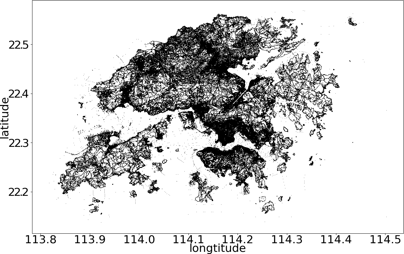
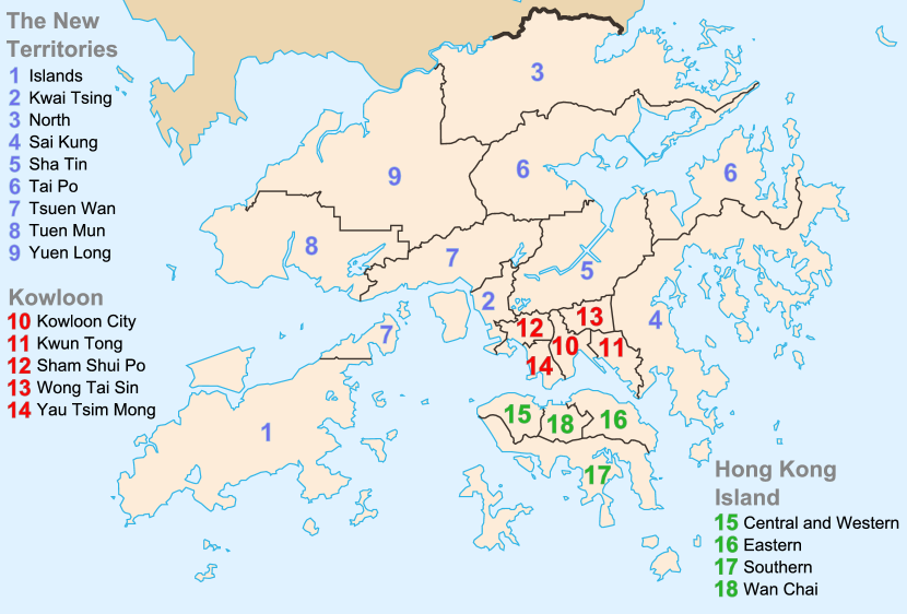
Figure 2: Demonstration of the data set. The 2D points extracted from [Ope17] are plotted on the left, next to a map of Hong Kong [Wik19] on the right.

Implementation

Recall that our coreset construction requires an initial center set $C$ that is an $O(1)$-approximation for the $p$-Centrum problem. However, $p$-Centrum is NP-hard as it includes $k$-Center (which is NP-hard even for points in $\mathbb{R}^{2}$), and polynomial-time $O(1)$-approximation algorithms known for it [BSS18, CS18b] are either not efficient enough for our large data set or too complicated to implement. Our experiments deal with an easier problem (small $k$ and points in $\mathbb{R}^{2}$), but since we are not aware of a good algorithm for it, our implementation employs instead the following simple heuristic: sample random centers from the data points multiple times, and take the sample with the best (smallest) objective value.

Our first experiment evaluates the performance of this heuristic. The results in Figure 3 show that 30 samples suffice to obtain a good solution for our data set. The rest the algorithm is implemented following the description in Section 4, while relying on the above heuristic as if it achieves $O(1)$-approximation. Thus, the experiments in this section for various $\epsilon$, $p$ and $k$, all evaluate a version of the algorithm that uses the heuristic.

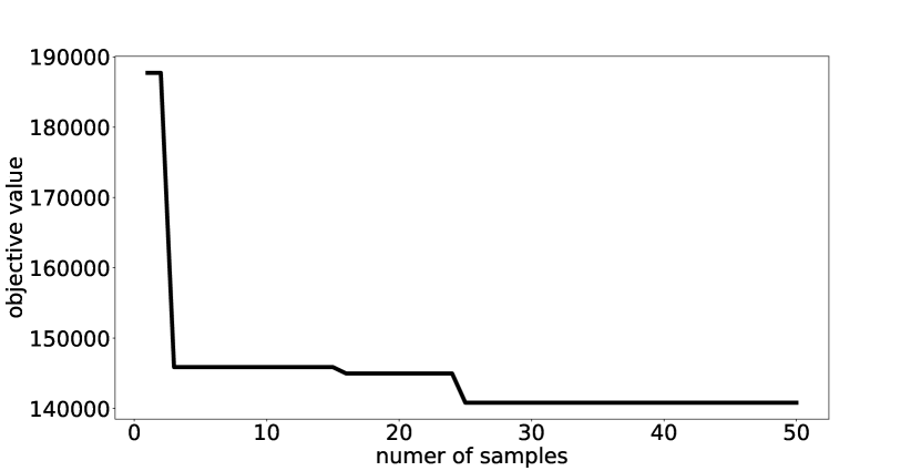
(a) $p=n$, $k=2$

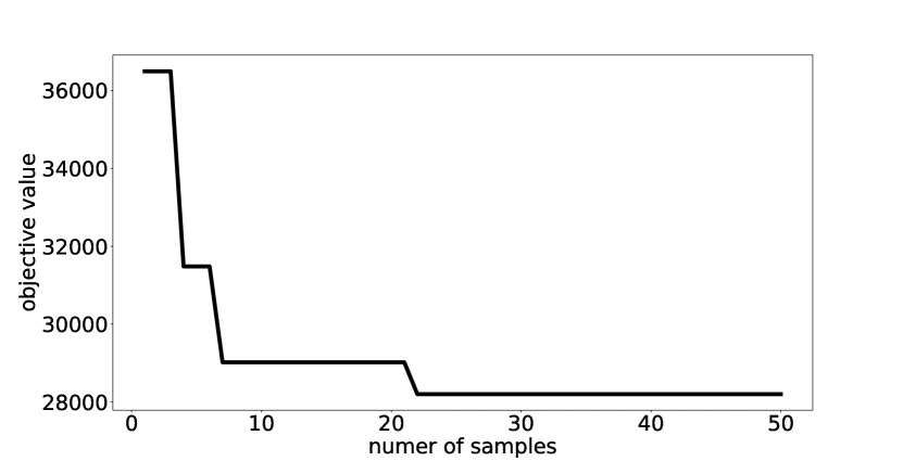
(b) $p=0.1n$, $k=2$

Figure 3: Performance of our $p$-Centrum heuristic, which takes the best of multiple randomly sampled centers.

Performance Evaluation

To examine the performance of our coreset algorithm for $p$-Centrum (using the heuristic for the initial centers), we execute it with parameters $p=0.1n$ and $k=2$, and let the error guarantee $\epsilon$ vary, to see how it affects the empirical size and error of the coreset. To evaluate the empirical error, we sample 100 random centers (each consisting of $k=2$ points) from inside the bounding box of the data set, and take the maximum relative error, where the relative error of coreset $X^{\prime}$ on centers $C$ is defined as $\left|\frac{\mathrm{cost}(X^{\prime},C)}{\mathrm{cost}(X,C)}-1\right|$ (similarly to how we measure $\epsilon$). We report also the total running time for computing the objective for the above mentioned 100 random centers, comparing between the original data set $X$ and on the coreset $X$’, denoted by $T_{X}$ and $T_{X}^{\prime}$, respectively. All our experiments were conducted on a laptop computer with an Intel 4-core 2.8 GHz CPU and 64 GB memory. The algorithms are written in Java programming language and are implemented single threaded.

These experiments are reported in Table 1. It is easily seen that the empirical error is far lower than the error guarantee $\epsilon$ (around half), even though we used the simple heuristic for the initial centers. Halving $\epsilon$ typically doubles the coreset size, but overall the coreset size is rather small, and translates to a massive speedup (more than 500x) in the time it takes to compute the objective value. Such small coresets open the door to running on the data set less efficient but more accurate clustering algorithms.

Table 1: Comparing coresets constructed for varying $\epsilon$ (and the same $p=0.1n$ and $k=2$).

$\epsilon$	emp. err.	coreset size	$T_{\text{X}}$ (ms)	$T_{\text{X'}}$ (ms)
50%	17.9%	122	143910	16
30%	14.3%	256	147216	15
20%	10.6%	475	131718	16
10%	7.0%	1603	134512	63
5%	2.8%	5385	130633	203

In Theorem 4.6, making the coreset work for all $p$ values incurs an $O(\log^{2}n)$ factor in the coreset size (see Section 4). We thus experimented whether a single coreset $X^{\prime}$, that is constructed for parameters $p=0.1n$, $\epsilon=10\%$, and $k=2$, is effective for a wide range of values of $p^{\prime}\neq p$. As seen in Table 2(a), this single coreset achieves low empirical errors (without increasing the size). We further evaluate this same coreset $X^{\prime}$ (with $p=0.1n$) for weight vectors $w$ that satisfy a power law (instead of 0/1 vectors). In particular, we let $w_{i}=\frac{1}{i^{\alpha}}$ for $\alpha>0$, and experiment with varying $\alpha$. The empirical errors of this coreset, reported in Table 2(b), are worse than that in Table 2(a) and is sometimes slightly larger than the error guarantee $\epsilon=10\%$, but it is still well under control. Thus, $X^{\prime}$ serves as a simultaneous coreset for various weight vectors, and can be particularly useful in the important scenario of data exploration, where different weight parameters are experimented with.

Table 2: Evaluating a single coreset (constructed for $\epsilon=10\%$, $p=0.1n$, $k=2$) for varying $p^{\prime}$ and for varying power-law weights.

(a) varying $p^{\prime}$

$p^{\prime}$	emp. err.
$0.01n$	4.0%
$0.05n$	6.6%
$0.2n$	5.0%
$0.3n$	4.1%
$0.4n$	3.6%
$0.5n$	3.3%
$n$	4.5%

(b) power-law weights

$\alpha$	emp. err.
0.5	3.2%
1.0	9.0%
1.5	11.1%
2.0	11.5%
2.5	11.6%
3.0	11.7%
3.5	11.7%

References

- [AHPV04] P. K. Agarwal, S. Har-Peled, and K. R. Varadarajan. Approximating extent measures of points. J. ACM, 51(4):606–635, July 2004. doi:10.1145/1008731.1008736.
- [AHV05] P. K. Agarwal, S. Har-Peled, and K. R. Varadarajan. Geometric approximation via coresets. In Combinatorial and computational geometry, volume 52 of MSRI Publications, pages 1–30. Cambridge University Press, 2005. Available from: http://library.msri.org/books/Book52/.
- [AP02] P. K. Agarwal and C. M. Procopiuc. Exact and approximation algorithms for clustering. Algorithmica, 33(2):201–226, 2002.
- [AS18] A. Aouad and D. Segev. The ordered k-median problem: surrogate models and approximation algorithms. Mathematical Programming, pages 1–29, 2018.
- [BCN19] S. K. Bera, D. Chakrabarty, and M. Negahbani. Fair algorithms for clustering. CoRR, abs/1901.02393, 2019. arXiv:1901.02393.
- [BHPI02] M. Bādoiu, S. Har-Peled, and P. Indyk. Approximate clustering via core-sets. In Proceedings of the Thiry-fourth Annual ACM Symposium on Theory of Computing, STOC ’02, pages 250–257. ACM, 2002. doi:10.1145/509907.509947.
- [BLL18] O. Bachem, M. Lucic, and S. Lattanzi. One-shot coresets: The case of -clustering. In AISTATS, volume 84 of Proceedings of Machine Learning Research, pages 784–792. PMLR, 2018. Available from: http://proceedings.mlr.press/v84/bachem18a.html.
- [BSS18] J. Byrka, K. Sornat, and J. Spoerhase. Constant-factor approximation for ordered -median. In Proceedings of the 50th Annual ACM SIGACT Symposium on Theory of Computing, pages 620–631. ACM, 2018. doi:10.1145/3188745.3188930.
- [CBK09] V. Chandola, A. Banerjee, and V. Kumar. Anomaly detection: A survey. ACM Comput. Surv., 41(3):15:1–15:58, 2009.
- [Che09] K. Chen. On coresets for -Median and -Means clustering in metric and Euclidean spaces and their applications. SIAM J. Comput., 39(3):923–947, August 2009. doi:10.1137/070699007.
- [CKLV17] F. Chierichetti, R. Kumar, S. Lattanzi, and S. Vassilvitskii. Fair clustering through fairlets. In NIPS, pages 5036–5044, 2017. Available from: http://papers.nips.cc/paper/7088-fair-clustering-through-fairlets.
- [CS18a] D. Chakrabarty and C. Swamy. Approximation algorithms for minimum norm and ordered optimization problems. arXiv preprint arXiv:1811.05022, 2018. arXiv:1811.05022.
- [CS18b] D. Chakrabarty and C. Swamy. Interpolating between -Median and -Center: Approximation Algorithms for Ordered -Median. In 45th International Colloquium on Automata, Languages, and Programming (ICALP 2018), volume 107 of Leibniz International Proceedings in Informatics (LIPIcs), pages 29:1–29:14. Schloss Dagstuhl–Leibniz-Zentrum fuer Informatik, 2018. doi:10.4230/LIPIcs.ICALP.2018.29.
- [FFM+15] M. Feldman, S. A. Friedler, J. Moeller, C. Scheidegger, and S. Venkatasubramanian. Certifying and removing disparate impact. In Proceedings of the 21th ACM SIGKDD International Conference on Knowledge Discovery and Data Mining, KDD ’15, pages 259–268. ACM, 2015. doi:10.1145/2783258.2783311.
- [FL11] D. Feldman and M. Langberg. A unified framework for approximating and clustering data. In Proceedings of the Forty-third Annual ACM Symposium on Theory of Computing, STOC ’11, pages 569–578. ACM, 2011. doi:10.1145/1993636.1993712.
- [FMSW10] D. Feldman, M. Monemizadeh, C. Sohler, and D. P. Woodruff. Coresets and sketches for high dimensional subspace approximation problems. In Proceedings of the Twenty-first Annual ACM-SIAM Symposium on Discrete Algorithms, SODA ’10, pages 630–649, Philadelphia, PA, USA, 2010. Society for Industrial and Applied Mathematics. Available from: http://dl.acm.org/citation.cfm?id=1873601.1873654.
- [FSS13] D. Feldman, M. Schmidt, and C. Sohler. Turning big data into tiny data: Constant-size coresets for k-means, pca and projective clustering. In Proceedings of the Twenty-fourth Annual ACM-SIAM Symposium on Discrete Algorithms, SODA ’13, pages 1434–1453. SIAM, 2013. doi:10.1137/1.9781611973105.103.
- [HK07] S. Har-Peled and A. Kushal. Smaller coresets for -median and -means clustering. Discrete & Computational Geometry, 37(1):3–19, 2007.
- [HM04] S. Har-Peled and S. Mazumdar. On coresets for -means and -median clustering. In 36th Annual ACM Symposium on Theory of Computing,, pages 291–300, 2004. doi:10.1145/1007352.1007400.
- [LS10] M. Langberg and L. J. Schulman. Universal epsilon-approximators for integrals. In SODA, pages 598–607. SIAM, 2010.
- [MS84] N. Megiddo and K. Supowit. On the complexity of some common geometric location problems. SIAM Journal on Computing, 13(1):182–196, 1984. doi:10.1137/0213014.
- [MS18] A. Munteanu and C. Schwiegelshohn. Coresets-methods and history: A theoreticians design pattern for approximation and streaming algorithms. KI, 32(1):37–53, 2018. doi:10.1007/s13218-017-0519-3.
- [Ope17] OpenStreetMap contributors. Planet dump retrieved from https://planet.osm.org . https://www.openstreetmap.org, 2017.
- [Phi16] J. M. Phillips. Coresets and sketches. CoRR, abs/1601.00617, 2016. arXiv:1601.00617.
- [RS18] C. Rösner and M. Schmidt. Privacy Preserving Clustering with Constraints. In 45th International Colloquium on Automata, Languages, and Programming (ICALP 2018), volume 107 of Leibniz International Proceedings in Informatics (LIPIcs), pages 96:1–96:14. Schloss Dagstuhl–Leibniz-Zentrum fuer Informatik, 2018. doi:10.4230/LIPIcs.ICALP.2018.96.
- [SSS18] M. Schmidt, C. Schwiegelshohn, and C. Sohler. Fair coresets and streaming algorithms for fair k-means clustering. CoRR, abs/1812.10854, 2018. arXiv:1812.10854.
- [SW18] C. Sohler and D. P. Woodruff. Strong coresets for k-median and subspace approximation: Goodbye dimension. In FOCS, pages 802–813. IEEE Computer Society, 2018.
- [Tam01] A. Tamir. The -centrum multi-facility location problem. Discrete Applied Mathematics, 109:293–307, 2001. doi:10.1016/S0166-218X(00)00253-5.
- [Wik19] Wikipedia contributors. Hong kong — Wikipedia, the free encyclopedia, 2019. [Online; accessed 18-January-2019]. Available from: https://en.wikipedia.org/w/index.php?title=Hong_Kong&oldid=878626680.
- [Yag88] R. R. Yager. On ordered weighted averaging aggregation operators in multicriteria decisionmaking. IEEE Trans. Syst. Man Cybern., 18(1):183–190, 1988. doi:10.1109/21.87068.