Computation of Chebyshev Polynomials for Union of Intervals
Simon Foucart111The research of the first author is partially funded by the NSF grants DMS-1622134 and DMS-1664803. (Texas A&M University) and Jean Bernard Lasserre222The research of the second author is funded by the European Research Council (ERC) under
the European Union’s Horizon 2020 research and innovation program (grant agreement 666981 TAMING). (LAAS-CNRS)
Abstract
Chebyshev polynomials of the first and second kind for a set are monic polynomials with minimal - and -norm on ,
respectively.
This articles presents numerical procedures based on semidefinite programming to compute these polynomials in case is a finite union of compact intervals.
For Chebyshev polynomials of the first kind,
the procedure makes use of a characterization of polynomial nonnegativity.
It can incorporate additional constraints,
e.g. that all the roots of the polynomial lie in .
For Chebyshev polynomials of the second kind,
the procedure exploits the method of moments.
Key words and phrases: Chebyshev polynomials of the first kind,
Chebyshev polynomials of the second kind, nonnegative polynomials, method of moments, semidefinite programming.
AMS classification: 31A15, 41A50, 90C22.
1 Introduction
The th Chebyshev polynomial for a compact infinite subset of is defined as the monic polynomial of degree with minimal max-norm on .
Its uniqueness is a straightforward consequence of the uniqueness of best polynomial approximants to a continuous function (here ) with respect to the max-norm, see e.g. [4, p. 72, Theorem 4.2].
We shall denote it as , i.e.,
(1)
We reserve the notation for the Chebyshev polynomial normalized to have max-norm equal to one on , i.e.,
(2)
With this notation, the usual th Chebyshev polynomial (of the first kind) satisfies
(3)
Chebyshev polynomials for a compact subset of play an important role in logarithmic potential theory.
For instance, it is known that the capacity of
is related to the Chebyshev numbers via
(4)
see [12, p.163, Theorem 3.1] for a weighted version of this statement.
The articles [1, 2] recently studied in greater detail the asymptotics of the convergence (4) in case is a subset of .
This being said, the capacity is in general hard to determine
— it can be found explicitly in a few specific situations,
e.g. when is the inverse image of an interval by certain polynomials
(see [8, Theorem 11]),
and otherwise some numerical methods for computing the capacity have been proposed in [11],
see also Section 5.2 of [10].
As for the Chebyshev polynomials, one is tempted to anticipate a worse state of affairs.
However, this is not the case for the situation considered in this article,
i.e., when is a finite union of compact intervals333The assumption is not restrictive,
as any compact subset of can be moved into the interval by an affine transformation.,
say
(5)
There are explicit constructions of Chebyshev polynomials (as orthogonal polynomials with a predetermined weight, see [9, Theorem 2.3]),
albeit only under the condition that is a strict Chebyshev polynomial
(meaning that it possesses points of equioscillation on
— a condition which is verifiable a priori, see [9, Theorem 2.5]).
Chebyshev polynomials can otherwise be computed using Remez-type algorithms for finite unions of intervals, see [5].
A first contribution of this article is to put forward an alternative numerical procedure that enables the accurate computation of the Chebyshev polynomials
whenever is a finite union of compact intervals.
The procedure, based on semidefinite programming as described in Section 2, can also incorporate a weight (i.e., a continuous and positive function on ), restricted here to be a rational function,
and output the polynomials
(6)
An appealing feature of this approach is that extra constraints can easily be incorporated in the minimization of (6).
For instance, we will show how to compute the th restricted Chebyshev polynomial on ,
i.e., the monic polynomial of degree having all its roots in with minimal max-norm on .
A second contribution of this article is to propose another semidefinite-programming-based procedure to compute weighted Chebyshev polynomials of the second kind, so to speak.
By this, we mean polynomials444The uniqueness of is not necessarily guaranteed: in the unweighted case, one can e.g. check that the monic linear polynomials with minimal -norm on are all the , .
We will not delve into conditions ensuring uniqueness of in this article.
(7)
The restriction that the weight is a rational function is not needed here,
but this time the computation is only approximate.
Nonetheless, it produces lower and upper bounds for the genuine minimium .
Both bounds are proved to converge to the genuine minimum as a parameter grows to infinity.
Along the way,
we shall prove that the Chebyshev polynomial of the second kind for , if unique, has simple roots all lying inside .
The procedures for computing Chebyshev polynomials of the first and second kind have been implemented in matlab.
They rely on the external packages CVX (for specifying and solving convex programs [3])
and Chebfun (for numerically computing with functions [13]).
They can be downloaded from the authors’ webpage as part of the reproducible file accompanying this article.
2 Chebyshev polynomials of the first kind
With as in (5),
we consider a rational555We could also work with piecewise rational weight functions, but we choose not to do so in order to avoid overloading already heavy notation. weight function taking the form
(8)
where the polynomials and are positive on each .
We shall represent polynomials of degree at most by their Chebyshev expansions written as
(9)
In this way, finding the th Chebyshev polynomial of the first kind for with weight
amounts to solving the optimization problem
(10)
After introducing a slack variable ,
this is equivalent to the optimization problem
(11)
The latter constraints can be rewritten as
on , ,
i.e., as the two polynomial nonnegativity constraints
(12)
The key to the argument is now to exploit an exact semidefinite characterization of these constraints.
This is based on the following result,
which was established and utilized in [7], see Theorem 3 there.
Proposition 1.
Given and a polynomial of degree at most ,
the nonnegativity condition
(13)
is equivalent to the existence of semidefinite matrices , such that
(14)
where and .
In the present situation,
we apply this result to the polynomials required to be nonnegative on each .
With
(15)
we write the Chebyshev expansions of and of as
(16)
where is the matrix of the linear map transforming the Chebyshev coefficients of into the Chebyshev coefficients of .
Our considerations can now be summarized as follows.
Theorem 2.
The th Chebyshev polynomial for the set given in (5) and with weight given in (8) has Chebyshev coefficients that solve the semidefinite program
(17)
where
and .
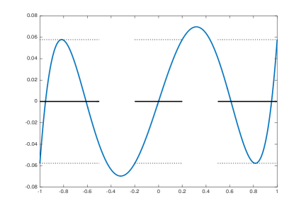
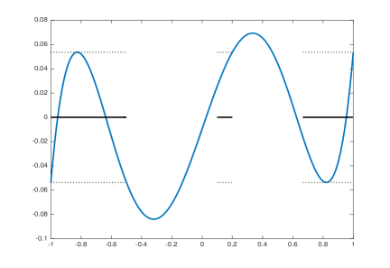
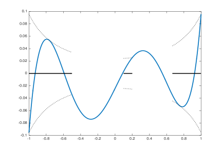
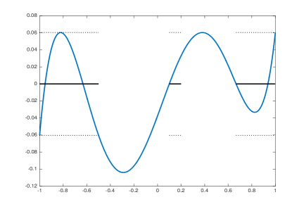
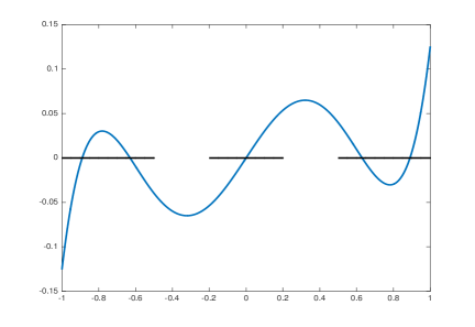
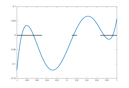
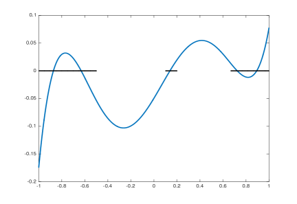
Figure 1 provides examples of Chebyshev polynomials of degree for the union of intervals which were computed by solving (17).
In all cases, the Chebyshev polynomials equioscillate times between and on , as they should.
However, they are not strict Chebyshev polynomials,
since the number of equioscillation points on is smaller than .
We notice in (c) and (d) that some roots of the Chebyshev polynomials do not lie in the set .
We display in (e) and (f) the restricted Chebyshev polynomial for ,
i.e., the monic polynomial of degree with minimal max-norm on which satisfies the additional constraint that all its roots lie in .
This constraint reads
(18)
We consider the semidefinite program (17) supplemented with the relaxed constraint
(19)
This is solved by selecting the smallest value (along with the corresponding minimizer) among the minima of semidefinite programs (17) indexed by ,
where the added constraint is the semidefinite characterization of the polynomial nonnegativity condition
(20)
One checks whether the selected minimizer satisfies the original constraint (18).
If it does,
then the restricted Chebyshev polynomial has indeed been found,
as in (e) and (f) of Figure 1.
(a)
(b)
, weighted
(c)
(d)
, weighted
(e)
, restricted
(f)
, restricted and weighted
Figure 1: th Chebyshev polynomials of the first kind for and for :
the first two rows correspond to the unrestricted case,
while restricted Chebyshev polynomials are shown in the last row;
the first column corresponds to the unweighted case,
while weighted Chebyshev polynomials with weight are shown in the second column.
Remark.
Concerning the computation of the capacity of a union of intervals,
we do not recommend using our semidefinite procedure or a Remez-type procedure to produce Chebyshev polynomials before invoking (4) to approximate the capacity.
If one really wants to take such a route,
it seems wiser to work with the numerically-friendlier orthogonal polynomials
(21)
Indeed, we also have
(22)
as a consequence of the inequalities
(23)
3 Chebyshev polynomials of the second kind
Still with as in (5),
but with an arbitrary (positive and continuous) weight function ,
we are now targeting th Chebyshev polynomials of the second kind for with weight ,
i.e.,
(24)
Let us drop the superscript and simply write for .
Minimizing the -norm on exactly seems out of reach,
so instead we shall perform the minimization of a more tractable ersatz norm,
which will be formally defined in Proposition 4.
This ersatz norm stems from a reformulation of the -norm on , as described in the steps below.
Given a polynomial of degree at most ,
we start by making two changes of variables to write
(25)
where and denote the functions and transplanted to , for instance
(26)
We continue by decomposing the signed measures as differences of two nonnegative measures, so that
(27)
where the infimum is taken over all nonnegative measures on .
As is well known, a minimization over nonnegative measures can be reformulated as a minimization over their sequences of moments.
There are several options to do so: here, emulating an approach already exploited in [6], see Section 3 there,
we rely on the discrete trigonometric moment problem encapsulated in the following statement.
Proposition 3.
Given a sequence ,
there exists a nonnegative measure on such that
(28)
if and only if the infinite Toeplitz matix build from is positive semidefinite, i.e.,
(29)
The latter means that all the finite sections of are positive semidefinite,
i.e.,
(30)
With representing the sequences of moments of ,
the objective function in (27) just reads
As for the constraints in (27),
with denoting the matrix of the linear map transforming the Chebyshev coefficients of into the Chebyshev coefficients of the second kind of ,
so that
(31)
they become, for all and all ,
(32)
where the infinite matrices have entries
(33)
The finite matrices , obtained by keeping the first rows of ,
are to be precomputed numerically and can sometimes even be determined explicitly,
e.g.
(34)
Taking into account the constraints that the must be sequences of moments,
we arrive at a semidefinite reformulation of the weighted -norm on given by
(35)
s.to
and
This expression is not tractable due to the infinite dimensionality of the optimization variables and constraints,
but truncating them to a level leads to a tractable expression — the above-mentioned ersatz norm.
Proposition 4.
For each , the expression
(36)
s.to
and
defines a norm on the space of polynomials of degree at most .
Moreover, one has
(37)
Proof.
To justify that the expression in (36) defines a norm,
we concentrate on the property ,
as the other two norm properties are fairly clear.
So, assuming that ,
there exist such that
(38)
as well as, for all ,
(39)
The semidefiniteness of the Toeplitz matrices implies that
(40)
which, in view of (38), yields .
By the invertibility of the matrices and the injectivity of the matrices (easy to check from (33)),
we derive that ,
and in turn that , as desired.
Let us turn to the justification of (37).
The chain of inequalities translates the fact that the successive minimizations impose more and more constraints,
hence produce larger and larger minima.
It remains to prove that the limit of the sequence equals (the limit exists, because the sequence is nondecreasing and bounded above).
For each ,
as was done in (38) and (39),
we consider minimizers of the problem (35)
—
they belong to but we pad them with zeros to create infinite sequences satisfying
(41)
as well as, for all ,
(42)
The semidefiniteness of the Toeplitz matrices,
together with (41),
implies that, for all ,
(43)
In other words,
each sequence ,
with entries in the sequence space , is bounded.
The sequential compactness Banach–Alaoglu theorem guarantees the existence of convergent subsequences in the weak-star topology.
With denoting these subsequences and
denoting their limits,
the weak-star convergence implies that
(44)
Writing (42) for and passing to the limit reveals that the sequences are feasible for the problem (35).
Hence,
(45)
where the last equality relied on the fact that the nondecreasing and bounded sequence is convergent.
This concludes the justification of (37).
∎
Given , let us now consider ersatz th Chebyshev polynomials of the second kind for (a priori not guaranteed to be unique) defined by
(46)
It is possible to compute such a polynomial by solving the following semidefinite program:
(47)
s.to
and
The qualitative result below ensures that, as increases,
the ersatz Chebyshev polynomials approach genuine Chebyshev polynomials ,
which are themselves obtained by solving the following (unpractical) semidefinite program:
(48)
s.to
and
Theorem 5.
Any sequence of minimizers of (46)
admits a subsequence converging
(with respect to any of the equivalent norms on the space of polynomials of degree at most )
to a minimizer of (24).
Moreover, if (24) has a unique minimizer ,
then the whole sequence converges to ,
i.e.,
(49)
Proof.
We first prove that the minima of (46) converge monotonically to the minimum of (24),
i.e.,
(50)
The argument is quite similar to the proof of (37) in Proposition 4.
The chain of inequalities holds because more and more constraints are imposed.
Next, considering coefficients and
infinite sequences satisfying
(51)
as well as and, for all ,
(52)
the semidefiniteness of the Toeplitz matrices, together with (51), still implies that the sequences admit convergent subsequences in the weak-star topology,
so we can write
(53)
We note that
(54)
It is easy to see that the coefficients thus defined, together with the sequences , are feasible for the problem (48),
which implies that
Let us now prove that the sequence admits a subsequence converging to a minimizer of (24).
This sequence is bounded (with respect to any of the equivalent norms, e.g. ):
indeed,
as a consequence of (37) and (50), we have
.
Therefore, there is a subsequence
converging to some monic polynomial .
Let us assume that is not one of the minimizers of (24),
i.e., that .
In view of (37), we can choose large enough so that
(56)
Let us observe that,
with being fixed and
by virtue of (37) and (50),
which is of course a contradiction.
This implies that is a minimizer of (24), as expected.
Finally, in case (24) has a unique minimizer ,
we can establish (49) by contradiction.
Namely, if the sequence did not converge to ,
then we could construct a subsequence
converging to some monic polynomial .
Repeating the above arguments would imply that is a minimizer of (24), i.e., ,
providing the required contradiction.
∎
Theorem 5 does not indicate how to choose a priori in order to reach a prescribed accuracy for the distance between and .
However, for a given ,
we can assess a posteriori the distance between the ersatz minimum and the genuine minimum .
Indeed, on the one hand, the semidefinite program (47) produces while outputting ;
on the other hand, the weighted -norm can be computed once has been output.
These two facts provide lower and upper bounds for the unknown value ,
as stated by the quantitative result below.
Proposition 6.
For any , one has
(59)
hence the weighted -norm of on is approximated with a computable relative error of
(60)
Proof.
By the definition (24) of the genuine Chebyshev polynomial of the second kind,
we have
(61)
and by the definition (46) of the ersatz Chebyshev polynomial of the second kind, together with (37), we have
(62)
This establishes the bounds announced in (59).
We also notice that the relative error satisfies
(63)
since, according to (49) and (50),
both and converge to
in case of uniqueness of .
In case of nonunuqueness, (63) remains true at least for a subsequence.
∎
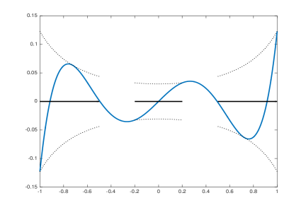
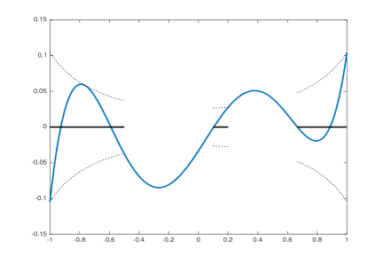
Figure 2 shows ersatz Chebyshev polynomials of the second kind computed on the same examples as in Figure 1.
Notice that no ‘restricted’ ersatz Chebyshev polynomials of the second kind are displayed.
This is because our experiments suggested that the polynomials had simple roots all lying inside .
The corresponding statement for the polynomials , in case of uniqueness, can in fact be justified theoretically by the following observation.
Proposition 7.
Let be a weighted Chebyshev polynomial of the second kind for a finite union of closed intervals .
This polynomial is the unique minimizer of (24) if and only if it has simple roots all lying inside .
Proof.
As a minimizer of (24),
a Chebyshev polynomial of the second kind for is characterized (see e.g. [4, p. 84, Theorem 10.4]) by the condition
(64)
This implies that has roots in ,
as (64) would not hold for
if had roots in .
Moreover, if one of the roots was repeated,
we would have for some polynomial of degree ,
but then (64) would not hold for this either.
Thus, the polynomial can be written, with distinct , as
(65)
Assume that is the unique Chebyshev polynomial of the second kind for .
If one of the ’s does not lie inside ,
i.e., if belongs to one of the gaps ,
then we can perturb to while keeping it in .
Hence, the perturbed monic polynomial
(66)
still satisfies for all .
The condition (64) is then fulfilled by , too,
so this monic polynomial is another minimizer of (24), which is impossible.
We have therefore proved that the simple roots of all lie inside .
Conversely, assume that has simple roots all lying inside
and let us prove that is the unique minimizer of (24).
Consider a monic polynomial
with .
In view of (64), we notice that
(67)
From here,
it follows that
(68)
The first and the last terms being equal,
we must have equality all the way through,
which means that for all .
Given that the polynomial vanishes at distinct points inside ,
the polynomial must also vanish at ,
and since both polynomials are monic,
we must have ,
proving the uniqueness.
∎
(a)
:
(b)
, weighted:
(c)
:
(d)
, weighted: ]
Figure 2:
Ersatz th Chebyshev polynomials of the second kind for and for :
the first column corresponds to the unweighted case,
while weighted ersatz Chebyshev polynomials with weight are shown in the second column.
References
[1]
J. Christiansen, B. Simon, and M. Zinchenko.
Asymptotics of Chebyshev polynomials, I: subsets of .
Inventiones Mathematicae 208.1 (2017): 217–245.
[2]
J. Christiansen, B. Simon, P. Yuditskii, and M. Zinchenko.
Asymptotics of Chebyshev polynomials, II: DCT subsets of .
Duke Mathematical Journal 168.2 (2019): 325–349.
[3]
CVX Research, Inc.
CVX: matlab software for disciplined convex programming, version 2.1 (2017).
http://cvxr.com/cvx
[4]
R. A. DeVore and G. G. Lorentz.
Constructive Approximation.
Vol. 303. Springer Science & Business Media, 1993.
[5]
S.-I. Filip.
A robust and scalable implementation of the Parks-McClellan algorithm for designing FIR filters.
ACM Transactions on Mathematical Software (TOMS) 43.1 (2016): 7.
[6]
S. Foucart and J. Lasserre.
Determining projection constants of univariate polynomial spaces.
Journal of Approximation Theory 235 (2018): 74–91.
[7]
S. Foucart and V. Powers.
Basc: constrained approximation by semidefinite programming.
IMA Journal of Numerical Analysis 37.2 (2017): 1066–1085.
[8]
J. Geronimo and W. Van Assche.
Orthogonal polynomials on several intervals via a polynomial mapping.
Transactions of the American Mathematical Society 308.2 (1988): 559–581.
[9]
F. Peherstorfer.
Orthogonal and extremal polynomials on several intervals.
Journal of Computational and Applied Mathematics 48.1-2 (1993): 187–205.
[10]
T. Ransford.
Potential Theory in the Complex Plane.
Vol. 28. Cambridge University Press, 1995.
[11]
T. Ransford and J. Rostand.
Computation of capacity.
Mathematics of Computation 76.259 (2007): 1499–1520.
[12]
E. Saff and V. Totik.
Logarithmic Potentials with External Fields.
Vol. 316. Springer Science & Business Media, 2013.
[13]
L. N. Trefethen et al.
Chebfun Version 5, The Chebfun Development Team (2017).
http://www.chebfun.org