Adaptive Fault Detection exploiting Redundancy with Uncertainties in Space and Time

Abstract

Abstract. The Internet of Things (IoT) connects millions of devices of different cyber-physical systems (CPSs) providing the CPSs additional (implicit) redundancy during runtime. However, the increasing level of dynamicity, heterogeneity, and complexity adds to the system’s vulnerability, and challenges its ability to react to faults. Self-healing is an increasingly popular approach for ensuring resilience, that is, a proper monitoring and recovery, in CPSs. This work encodes and searches an adaptive knowledge base in Prolog/ProbLog that models relations among system variables given that certain implicit redundancy exists in the system. We exploit the redundancy represented in our knowledge base to generate adaptive runtime monitors which compares related signals by considering uncertainties in space and time. This enables the comparison of uncertain, asynchronous, multi-rate and delayed measurements. The monitor is used to trigger the recovery process of a self-healing mechanism. We demonstrate our approach by deploying it in a real-world CPS prototype of a rover whose sensors are susceptible to failure.

1 Introduction

Cyber-physical systems (CPSs) are desired to be resilient (i.e., dependable and secure) against different kinds of faults throughout its lifecycle. Failure scenarios like communication crashes and dead batteries (fail-silent, fail-stop) are easy to handle (watchdog/timeout). However, sensor data may be erroneous due to noise (e.g., communication line, aging), environmental influences (e.g., dirtying, weather) or a security breach. To detect a sensor failure one has to define a valid signature [1, 2, 3, 4] or specification [5, 6] or create particular failure models [7, 8] for each possible hazard (c.f., aging, dirtying and a security breach). A simple method for detecting a faulty sensor value in different failure scenarios is to check against related information sources, i.e., exploit redundancy. Explicit redundancy, that is replicating the sensor [9, 10] is costly.

A designed system might not incorporate (implicit) redundancy straightaway (if so, the system would use information fusion to exploit the redundancy). However, when assembling (sub-)systems of different suppliers redundancy often becomes available. This is typically the case for distributed systems like the Internet of Things (IoT) or a Cyber-Physical System (CPS). For instance, the drivetrain of an electric vehicle is equipped with several sensors at the battery, motor, transmission, shaft, differential, or wheels level. The physical entities (CPS variables) observed in these subsystems, e.g., power consumption, revolution, speed or torque, are all related to the velocity of the vehicle, thus providing implicit information redundancy [11, 12].

We exploit such implicit redundancy by encoding it in a knowledge base [11, 13] created by domain experts or learned during runtime. Our previous work [14] shows how to use the redundancy to substitute failed observation components. We refer to it as Self-Healing by Structural Adaptation (SHSA). The SHSA service acts independently of the application on the communication network of the system. However, it needs a monitor to trigger the recovery from failures.

This work exploits the SHSA knowledge base to monitor related information. Similar solutions [15, 16, 17] perform the comparison synchronously, that is, all measurements are assumed to have the same timestamp (and therefore can be safely compared against each other). However, typically the runtime monitor has to cope with asynchronous, multi-rate and delayed measurements. Moreover, the timestamp of a measurement might not express the time when the CPS variable actually adopted this value (time-delay system). Typical runtime monitors are statically configured and therefore cannot cope with changes of a dynamic and evolving system (e.g., availability of signals, message structure of the observations).

We therefore propose an observation model based on interval arithmetic considering uncertainties in space and time and an adaptive method to compare such signals. In particular, our novel contributions are as follows:

• A short, adaptive and extensible implementation of the knowledge base in Prolog/ProbLog.

• A simple model for observations of a signal that is prone to uncertainties in space and time.

• The generation of adaptive runtime monitors for signals which compare uncertain, asynchronous, multi-rate and/or delayed observations.

• Demonstration of our method on a real-world application – an implementation on a rover prototype that performs collision avoidance.

The rest of the paper is organized as follows. Section 2 gives an overview of related work. Section 3 introduces the running example of our mobile robot and defines the knowledge base. Section 4 encodes the knowledge base in Prolog. Section 5 describes the signal model and shows how a monitor is generated for comparing itoms. Section 6 demonstrates and tests the fault detection of the generated monitor. Section 7 concludes by summarizing our results and outlining the future work.

2 Related Work

In [11], Höftberger introduced an ontology (a knowledge base) defining physical relations or semantic equivalences between variables (e.g., laws of physics) to substitute failed observation services. We applied this technique in [14] and we extended the knowledge base with properties and utility theory in [13]. However, this knowledge base has been only exploited for failure recovery, but not yet for fault detection.

Literature on fault detection is spread to the area of runtime verification [5, 6], anomaly detection [1], intrusion detection [2, 3, 4], fault-tolerance [18, 19, 9, 20] and self-healing [21, 22]. Approaches to detect faults typically use a specification or signature, an anomaly model or redundancy as a reference to judge the behavior of an entity.

A popular approach to perform fault detection in safety critical systems is to exploit redundancy of components. Examples include lockstep [10] and triple modular redundancy (TMR) [9] that explicitly replicate software or hardware components to detect faults. In the best case the replicas are diverse, i.e., they have been separately designed but share the same functionality and interface, to avoid joint or concurrent failures. Replication is generally expensive because it requires additional time and resources both at design time and runtime.

The security framework described in [23] performs anomaly detection on input signals of a component in a distributed network by comparing the input against trusted local signals (if available). The local signals may be provided by sensors which are directly sampled by the component and not advertised in the vulnerable communication network (cf. IoT) of the system.

The proposed method in [15] votes over signals sent through transfer functions (cf. relations) of known or unknown relationships of signals. The difference between the signals raises an alert when it exceeds a threshold. Similarly, we use transfer functions (here: relations) to bring signals into a common domain before comparison.

The author of [16] uses ensemble modeling to represent the redundancy of data streams. First a dependency graph between data streams of nodes is created (via cross-correlation). An ensemble of estimators of the learned models is defined given a threshold on the cross-correlation. The estimators can be created from different types of models (e.g., linear functions or neural networks) to relate the data streams to each other (temporal and functional relationships in the physical layer). The output of the estimators are combined in a weighted-averaging fashion (cf. confidence-weighted averaging [24]). Another threshold for the estimator output defines whether an anomaly has occurred or not. However, the ensemble is statically defined during design time. The estimators have to be aggregated and weighted in a proper way. Similarly, the threshold is crucial to avoid false positives. Although time delays are not discussed, appropriate estimators can be set up to consider (at least constant) time delays.

The authors of [25] propose instead a Bayesian network (BN) with past and future values of sensor readings and redundant ones (spatial and temporal redundancy) to estimate the true state of a variable. A sensor is classified faulty, when its measurement exceeds a threshold given the estimated state. Similarly, fault injection is used to evaluate the monitoring technique. The proposed BN can be compared to a state estimator fusing redundant sensors.

References	Redundancy		Dynamic Systems	Uncertain Signals
	Explicit	Implicit		Space	Time
[10, 9]	✓
[23]	✓	✓
[15]		✓
[25]	✓			✓
[16]	✓	✓		✓
This work	✓	✓	✓	✓	✓

Table 1: Comparison of state-of-the-art fault detection using redundancy.

All related work listed in Table 1 considers constant variance of the signals, i.e., the threshold for mismatch is set a priori. By using intervals to express observations we can handle time-varying errors. Most of the related work assumes the signals to compare to be sampled at the same point in time, i.e., are truly comparable. A dynamic BN like proposed by [25] could relate asynchronous observations to each other by forward estimation given the timestamp of the observation. However, neither of the listed work discussed this issue. Our knowledge base resembles a Bayesian network (in particular the sensor model of a BN), similar to [16, 25], but with deterministic nodes (relations or transfer functions) that can be re-used, merged and adapted when components are added or removed from a dynamic system. However, for our needs the knowledge base expresses a set of rules (cf. relations) on how to compare signals or to substitute a failed signal.

3 Background

In this section we recap our knowledge base of redundancy and showcase it on a real-world prototype [13].

3.1 Running Example

The running example is a mobile robot (Pioneer 3-AT) that avoids collisions. Our rover under test (Fig. 1) is equipped with a Jetson TK1 and a Raspberry Pi 3 running the Robot Operating System (ROS) [26] and controlled via WiFi using a notebook. A ROS application can be distributed into several processes, so-called nodes which may run on different machines. Nodes communicate via a message-based interface over TCP/IP. In particular, ROS nodes subscribe and publish to ROS topics (cf. named channels). ROS can start new nodes and reconfigure the communication flow of existing nodes during runtime and it is therefore suitable for SHSA [14].

Figure 1: Mobile robot equipped with its sensors and processing units.

3.2 System Model

As our focus is on self-healing in the software cyber-part of a CPS $Z$ (cf. dynamic reconfiguration of an FPGA), we assume that each physical component comprises at least one software component $z$ (e.g., the driver of the LIDAR) and henceforth, consider the software components only.

A system $Z$ can be characterized by properties, referred to as system features, or simply as variables V (e.g., position of a vehicle, point cloud or distance measurements acquired by a LIDAR). In SHSA we focus on observations of CPS variables and refer to the actual data as value. A signal $v(t)$ or short $v$ represents the values of a variable $\mathsf{v}$ over time ($t\in\mathbb{R}$) provided by a certain component (e.g., a sensor).

The value of a system variable – an observation – is communicated between components typically via message-based interfaces. We denote such transmitted data representing the value of a variable $\mathsf{v}$, as information atom [27], short itom. In general, an itom is a tuple including data and an explanation of this data. An SHSA itom $v(t_{s})=(v,t_{s})$ is a sample or a snapshot of a variable at a certain point in time $t_{s}$. It provides the following explanation of the data: i) the associated variable or entity, and ii) the timestamp of the acquisition or generation of the value. Each itom is identified by its signal’s name $v$ and its timestamp. A variable can be provided by different components simultaneously (e.g., $p$ redundant sensors).

Each software component $z$ executes a program that uses input signals and provides output signals.

The CPS implements some functionality, a desired service (e.g., tracking). The subset of components implementing the CPS’ objectives are called controllers.

A signal $v$ is needed, when $v$ is input of a controller.

Case Study (Fig. 2): The rover is tele-operated by the controller $z_{notebook}$ publishing the desired velocity $v_{cmd}$. The distance to the nearest obstacle $\mathsf{v}_{dmin}$ is evaluated by the component $z_{dmin\_calc}$ using the LIDAR data as input. As soon as $v_{dmin}$ falls below a safety margin (for simplicity a constant value) the robot’s verified desired velocity $v_{safe\_cmd}$ is set to $0$. The component $z_{rover\_uc}$ applies $v_{safe\_cmd}$ to the motors and provides sonar range measurements $v_{sonar}$ and actual linear and angular velocity $v_{speed}$.

Another component $z_{tof}$ provides 3D images of the environment in front of the rover. However, dashed signals in Fig. 2 are not used for collision avoidance but available for other tasks (e.g., parking, object recognition).

Figure 2: Relevant application components and signals of the mobile robot.

3.3 Input Interface of Components

The messages communicated within the network may be received synchronously or asynchronously. In our rover like in many other IoT infrastructures, the communication is asynchronous, i.e., the exact point in time of a message reception is unknown. The task of the component might be executed when an itom is received (e.g., $z_{dmin\_calc}$ calculating minimum distance when receiving $v_{lidar}$). However, the inputs of a software component might be published with different rates. Some components therefore have to cope with multi-rate, asynchronous and late messages. The monitor described in Sec. 5 periodically executes the plausibility check using the itoms collected since the last monitor call and a (configurable sized) buffer of itoms of previous executions.

3.4 Knowledge Base of Redundancy

This section defines the knowledge base used to describe implicit redundancy [13].

3.4.1 Variables and Relations

Variables are related to each other. A relation $\mathsf{r}:\mathsf{v}_{o}=f(\text{V}_{I})$ is a function or program (e.g., math, pseudo code or executable python code) to compute an output variable $\mathsf{v}_{o}$ from a set of input variables $\text{V}_{I}$. The relations can be defined by the application’s domain expert or learned (approximated) with neural networks, SVMs or polynomial functions (see [14]).

3.4.2 Structure

The knowledge base $K=(\text{V},\text{R},E)$ is a bipartite directed graph (which may also contain cycles) with independent sets of variables V and of relations R of a CPS. V and R are the nodes of the graph. Edges $E$ specify the input/output interface of a relation. In particular, $\mathsf{v}_{i}$ is an input variable for $\mathsf{r}$ iff $\exists(\mathsf{v}_{i},\mathsf{r})\in E$ denoted as $\mathsf{v}_{i}\xrightarrow{e}\mathsf{r}$. $\mathsf{v}_{o}$ is the output variable of $\mathsf{r}$ iff $\exists(\mathsf{r},\mathsf{v}_{o})\in E$ denoted as $\mathsf{r}\xrightarrow{e}\mathsf{v}_{o}$. $Pred_{Y}(x)$ denotes the predecessors of a node $x$ in graph $Y$. There are no bidirectional edges, i.e., if $\mathsf{v}_{i}\xrightarrow{e}\mathsf{r}\Rightarrow{\not\exists}\mathsf{r}\xrightarrow{e}\mathsf{v}_{i}$. Hence a variable is either input or output to a relation, but never both. A relation can further have only one output variable, i.e., for $\forall j\neq i$ if $\mathsf{r}\xrightarrow{e}\mathsf{v}_{i}\Rightarrow{\not\exists}\mathsf{r}\xrightarrow{e}\mathsf{v}_{j}$. Note that relations have to be modeled as nodes, not edges, because a variable is typically related to more than one variable via a single relation.

Case Study: The application nodes of the rover (Fig. 2) provide several observation signals. The relations of the signals, that is the knowledge base, are set up manually (Fig. 3).

Figure 3: Knowledge base of the mobile robot depicting relations exploitable for collision avoidance. Boxes are relations. Ellipses are variables. Variables are annotated with available signals (from Figure 2).

3.4.3 Substitution

A substitution $s$ of $\mathsf{v}_{sink}$ is a connected acyclic sub-graph of the knowledge base with the following properties: i) The output variable is the only sink of the substitution (acyclic + Eq. 2). ii) Each variable has zero or one relation as predecessor (Eq. 3). iii) All input variables of a relation must be included (Eq. 4; it follows that the sources of the substitution graph are variables only).

$$s=(\text{V}_{s},\text{R}_{s},E_{s})$$ (1)

$$\mathsf{v}_{sink}\in\text{V}_{s},\text{V}_{s}\subseteq\text{V},\text{R}_{s}\subseteq\text{R},E_{s}\subseteq E$$

$$\forall x\in\text{R}_{s}\cup\text{V}_{s}\setminus\mathsf{v}_{sink}\quad\exists y\in\text{R}_{s}\cup\text{V}_{s}\;|\;\exists x\xrightarrow{e\in E_{s}}y$$ (2)

$$\forall\mathsf{v}\in\text{V}_{s}\quad|Pred_{s}(\mathsf{v})|\leq 1$$ (3)

$$\forall\mathsf{r}\in\text{R}_{s}\quad\forall\mathsf{v}\in Pred_{K}(\mathsf{r})\;|\;\mathsf{v}\in\text{V}_{s}$$ (4)

A substitution $s$ is valid if all sources are provided, otherwise the substitution is invalid. We denote the set of valid substitutions of a variable $\mathsf{v}$ as $S(\mathsf{v})$. Only a valid substitution can be instantiated by concatenating the relations $\text{R}_{s}$ to the function $f_{s}$ which takes selected signals $I_{s}$ as input.

Case Study: When $v_{dmin}$ fails it can be replaced by the outputs of the substitution in Figure 4, by using the provided signal $v_{tof}$ as input.

Figure 4: A valid substitution for $\mathsf{v}_{dmin}$.

4 SHSA in Prolog

A Prolog program is a set of facts, rules and queries. The formal definitions of SHSA given above can be efficiently (that is, with a few lines of code) expressed in Prolog. It is also a good basis to extend SHSA in future work, e.g., runtime adaptation of the knowledge base or validation of requirements for substitutions.

The structure of the knowledge base and availability of variables is defined by a set of Prolog facts (see example in Listing 1). In particular, a relation $\mathsf{r}:\mathsf{v}_{o}=f(\text{V}_{I})$ is written as the fact function(o,r,[i0,..,in]) with a list of names [i0,..,in] representing the input variables, a name of the relation r and the name of the output variable o. An itom i is available when the fact itom(i) evaluates to true. In addition, each itom has to be mapped to its corresponding variable. For convenience, the availability of a variable can be specified via a list of itoms, e.g., itomOf(v,[i0,..,in]). This implicitly maps each itom i* to the variable v and marks the variable v as provided(v) (provided is a Prolog property). The facts itomsOf(.) are added during runtime to the program (structure of the knowledge base) depending on the itoms gathered by the monitor.

Case Study: Listing 1 shows the knowledge base of Figure 3 in Prolog. Table 2 maps the knowledge base variables to Prolog names.

⬇

1:- use_module(library(shsa)).

2

3% structure

4function(dmin, r1, [d_2d]).

5function(d_2d, r2, [d_3d]).

6function(dmin, r3, [dmin_last, speed]).

7function(dmin_last, r4, [dmin]).

8

9% provided itoms

10itomsOf(dmin, ["/emergency_stop/dmin/data"]).

11itomsOf(d_2d, ["/p2os/sonar/ranges",

12 "/scan/ranges"]).

13itomsOf(d_3d, ["/tof_camera/frame/depth"]).

14itomsOf(speed, ["/p2os/cmd_vel",

15 "/p2os/odom"]).

Listing 1: Knowledge base of the mobile robot in Prolog.

Variable	Prolog	Signal	Prolog
$\mathsf{v}_{dmin}$	dmin	$v_{dmin}$	"/calculator/dmin"
$\mathsf{v}_{dmin^{\prime}}$	dmin_last	-	-
$\mathsf{v}_{speed}$	speed	$v_{speed}$	"/rover/act_vel"
		$v_{safe\_cmd}$	"/safe/cmd_vel"
$\mathsf{v}_{2D}$	d_2d	$v_{sonar}$	"/sonar/ranges"
		$v_{lidar}$	"/lidar/ranges"
$\mathsf{v}_{3D}$	d_3d	$v_{tof}$	"/tof/ranges"

Table 2: Used variable and signal names in Prolog.

The Prolog library shsa implements a set of rules to evaluate properties (e.g., SHSA properties of variables like provided(v).) or to search substitutions for a needed variable (query substitution(v,S).). It basically implements the definitions in the previous section within 22 lines of code. Details can be found in our repository .

Finally, we can query properties, e.g., substitution(v,S). to find all valid substitutions for the variable v. The Prolog engine (here: ProbLog[28]) tries to satisfy the query, that is, it searches for S which evaluates the query to true (“unify” S) considering the given facts (SHSA knowledge base) and rules (SHSA library). In this case, S is a relation or a tree of relations, see the substitute search for dmin in Listing 2.

⬇

1substitution(dmin,"/emergency_stop/dmin/data")

2substitution(dmin,[function(dmin,r1,[d_2d]),

3 "/scan/ranges"])

4substitution(dmin,[function(dmin,r1,[d_2d]),

5 "/p2os/sonar/ranges"])

6substitution(dmin,[function(dmin,r1,[d_2d]),

7 [function(d_2d,r2,[d_3d]),

8 "/tof_camera/frame/depth"]])

Listing 2: Evaluation result of the query substitution(dmin,S).

The complexity of the query is the one of a depth-first search, i.e., $O(b^{d})$ with the branching factor $b$ and depth $d$.

ProbLog provides a Python interface which makes it easy to interface with our existing application. Moreover, Python facilitates data (pre-)processing and enables the execution of arbitrarily complex code. We therefore parse the substitution results and execute these in Python.

To this end, each relation is linked to an implementation capturing a string that can be evaluated in Python (Listing 3).

⬇

1implementation(r1, "

2dmin.v = min(d_2d.v)

3dmin.t = d_2d.t

4").

5implementation(r2, "

6# row width of depth image

7w = 320

8# take 115th row (about the height of lidar scan)

9h = 115

10d_2d.v = [d for i, d in enumerate(d_3d.v)

11 if i >= h*w and i < (h+1)*w]

12d_2d.t = d_3d.t

13").

Listing 3: Python implementation of relations.

For instance, r1 passes the distance measurements d_2d.v through the function it should implement, here: min. The timestamp dmin.t is adopted from the distance measurements to indicate the time when the minimum distance occurred.

5 Fault Detection by Exploiting Redundancy

A generic monitor uses the knowledge base to setup a monitor for a given signal and to periodically compare against the related signals.

5.1 Setup and Adaptation

First, the monitor queries the valid substitutions $S(\mathsf{v})$ given the variable $\mathsf{v}$ to monitor and the available signals (Sec. 4). Then the monitor parses the result and instantiates the substitutions. Once set up, the monitor periodically executes the substitutions with the given input itoms and compares the outputs against each other.

On system changes, e.g., regarding the relations or the availability of signals, the knowledge base can be adapted and the monitor re-initialized. For instance, the knowledge base may be extended with new relations whenever new information becomes available (i.e., when new observation components are connected).

Case Study: The collision avoidance (controller $z_{safe}$) needs the signal $v_{dmin}$ which shall therefore be monitored. The setup is depicted in Figure 5. This monitor compares the output of 5 substitutions (including the empty substitution using the itoms of signal $v_{dmin}$ directly).

Figure 5: Check $v_{dmin}$ against redundancy. The itoms are first transferred into the common domain (here: $\mathsf{v}_{dmin}$) and compared against each other.

Note, that the substitutions should be diverse. For instance, an error in the LIDAR will cause errors in 3 substitutions including $v_{dmin}$ itself ($z_{calc}$ uses $v_{lidar}$ as input too).

5.2 Observation Model

Once the observations or itoms are in the common domain, their values can be compared to each other. However, the values are uncertain, e.g., due to noise, interference or environmental conditions (the accuracy of a LIDARs distance measurement for instance is sensitive to the reflexion capabilities of a surface).

In our proof-of-concept implementation we use simple integer arithmetic to express the allowed uncertainty of an itom or confidence into an itom. The value of the itom $v(t_{s})=(\boldsymbol{v},t_{s})$ is expressed as an interval (Eq. 5).

$$\boldsymbol{v} =[\underline{v},\overline{v}]=\{v\in\mathbb{R}^{2}\,|\,\underline{v}\leq x\leq\overline{v}\}$$ (5)

In real-world data, however, the itoms diverge not only in space but also in the time domain. This phenomenon is known as dead-time or aftereffect and occurs in time-delay systems [29]. Delays may accumulate from different sources, not only from communication latency. For instance, the travel of sound is slower than the travel of light. So the sonar sensor of a mobile robot will react slower to changes in the distance than a laser scanner. The time shifts can be estimated, e.g., by using the Skorokhod distance [30]. However, the delay of the sonar measurement depends on the distance measured, i.e., the time delay is not constant.

We therefore distinguish between the time $t_{x}$, when the CPS variable actually adopted the value, the timestamp of the measurement $t_{s}$ included in the itom (typically the time when the message has been generated and provided by the sensor) and the time the itom is received $t_{r}$ or used $t_{cur}$ (here: by the monitor), depicted in Figure 6. Unfortunately, $t_{x}$ is unknown and typically does not match $t_{s}$ (though often the difference is neglectable). CPS variables are often sampled periodically. The sampling period $T$, i.e., the time between two consecutive itoms of a signal, should be small enough to follow the dynamics of the CPS variable under observation.

Figure 6: Timeline of an itom $v(t_{s})$.

Note that the timeline or the order of these timestamps are applicable in most CPSs, regardless of the type or implementation of the communication (e.g., synchronous or asynchronous). However, the results of the computation using the itom might get distorted, especially when $t_{s}\gg t_{x}$ (late time-stamping, e.g., due to insufficient sensor capabilities) or $T<(t_{r}-t_{s})$ (high communication latency, e.g., due to monitoring in the cloud).

For the above reasons, the monitor should not simply compare the last values received but consider the time delay (from $t_{x}$ to $t_{cur}$). Still the itom is the best (latest) the monitor can make use of (without much more effort like forward estimation). An itom is therefore considered valid for a time interval or time span (and not only at the given timestamp $t_{s}$ of the itom).

$$v(t_{s})=(\boldsymbol{v},\boldsymbol{t})\qquad \boldsymbol{v}=[\underline{v},\overline{v}]$$ (6)

$$\boldsymbol{t}=[\underline{t},\overline{t}]\quad t_{s}\in[\underline{t},\overline{t}]$$

An itom is typically late (e.g., acquired by a sensor), but it may be valid/useful into the future, i.e., the sampling time $t_{s}$ lies within the time span $\boldsymbol{t}$.

A variable $\mathsf{v}$ is provided at time $t_{cur}$ when at least one corresponding itom $\boldsymbol{v}(\boldsymbol{t})$ exists with $t_{cur}\in\boldsymbol{t}$.

Case Study: We set $\boldsymbol{t}=[t_{s}-\Delta,t_{s}]$ given the timestamp of the observation $t_{s}$ and a delay $\Delta$ which sums up the latencies caused by the sampling process, pre-processing (e.g., filtering) and communication. The size of the interval may match the sampling period $T$ of the signal to continuously have comparable values. Note, that a sensor should be able to follow the dynamics of the system ($T$ is small enough). Figure 7 visualizes two signals of the same variable and the confidence intervals of the latest itoms received by the monitor. For a one-dimensional itom the confidence region is a rectangle.

Figure 7: Two one-dimensional signals (itoms over time). The confidence regions of the latest itoms are highlighted.

The demonstration in Section 6 uses the specifications from sensors’ datasheets. For instance, we set the maximum delay $\Delta_{sonar}$ of the itoms provided by the array of $8$ sonar sensors to $8\cdot 10ms$, considering the maximum range of $3m$, the sonar speed of $343m/s$ and an average communication delay of $1ms$.

5.3 Comparison

Exceeding the threshold for an error is implicitly defined by the size of the intervals (in time and space). Overlapping confidence intervals indicate the itoms to be equal (Fig. 7), non-overlapping means the itoms diverge. It is a relative fast way to compare itoms (cf. itoms represented by a probability distribution), and therefore suitable for real-time systems.

The monitor is periodically ($T_{m}$) fed with the latest itoms. It may save previous itoms to compensate for late receptions, so a newly received, but delayed itom ($\boldsymbol{t}\ll t_{r}<t_{cur}$) can be compared to a past itom with similar time interval.

The total set of buffered itoms $I$ is used as inputs to the substitutions $S(\mathsf{v})$ to generate comparable (output) itoms. Two or more itoms are comparable when the itoms have a common corresponding variable and their time intervals overlap.

A monitor step consists of the following substeps:

• Collect combinations of input itoms $(\boldsymbol{v},\boldsymbol{t})$ per substitution $s\in S(\mathsf{v})$ such that their time intervals overlap and a combination $c$ contains exactly one itom per input signal $v\in I_{s}$ of $s$ (Cartesian product).

$$\forall s\in S(\mathsf{v}),\,v_{1},..,v_{m}\in I_{s}\colon$$

$$C_{s}=\{((\boldsymbol{v},\boldsymbol{t})_{1},\ldots,(\boldsymbol{v},\boldsymbol{t})_{m})\,|\,\cap_{i=1,..,m}\boldsymbol{t}_{i}\neq\emptyset\}$$

• Execute the substitutions to generate output itoms to compare against. The value interval of the input itoms $c\in C_{s}$ of a substitution $s$ are passed through the functions of $s$ giving the value interval of the output itom (see interval arithmetic [31]). The time interval of the output itom is the intersection of the time intervals of the inputs.

$$\forall s\in S(\mathsf{v}),\,\forall c\in C_{s}\colon$$

$$O=\{(s,(\boldsymbol{v},\boldsymbol{t}))\,|\,\boldsymbol{v}=\boldsymbol{f}_{s}(c),\,\boldsymbol{t}=\bigcap_{v_{i}\in c}\boldsymbol{t}_{i}\}$$

• Pairwise compare the output itoms $O$ to calculate an error matrix of the value intervals.

$$\forall(s,(\boldsymbol{v},\boldsymbol{t}))_{i},(s,(\boldsymbol{v},\boldsymbol{t}))_{j}\in O,\,i\neq j\colon$$

$$e_{s_{i}s_{j}}=\sum|max(\underline{v}_{i},\underline{v}_{j})-min(\overline{v}_{i},\overline{v}_{j})|$$

• Rank the error to return the substitution with the highest error. The errors per substitution are summed up (sum of columns or rows of the error matrix). When an error per substitution is greater than $0$ the monitor returns the failed substitution.

Case Study: The implementation uses pyinterval  to pass itoms through a substitution or to identify the pairs of itoms to compare. The size of the itoms buffer is a constant parameter of the monitor for simplicity. However, the monitor may increase the size of the buffer according to the observed delays ($t_{r}-t_{s}$).

6 Experiments

In this section we demonstrate the monitor setup and fault detection.

6.1 Setup

The demo uses the mobile robot described in Sec. 3. The hosts on the rover (connected via WiFi to the notebook) only run the sensor drivers, while the controllers and the monitor are executed on the notebook (Intel i7 2.1GHz x 4, 8GB RAM, Ubuntu, ROS and its nodes run in Docker containers).

The rover is tele-operated via the notebook towards a wall (Fig. 8). The ROS messages of the sensors (monitored inputs) and the monitor itself (failed substitution and additional debug output) are logged.

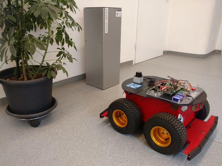
Figure 8: Images of the test scenario. The figure on the right depicts a ToF camera depth image. The line marked in red is used to compare against the laser scan.

6.2 Demonstration

Figure 9 depicts some application logs taken from a run of the demo. The rover first moves slowly and straight towards the wall ($t=2..5s$: $v_{dmin}$ slowly decreases). To test the possibly different delays of the sensors, a dynamic obstacle has been placed in front of the rover for some period of time ($t=5..8s$: $v_{dmin}$ falls below a threshold, robot stops). Finally, the rover reaches the wall ($t=17..20s$) and goes back relatively fast ($t=20..23s$).

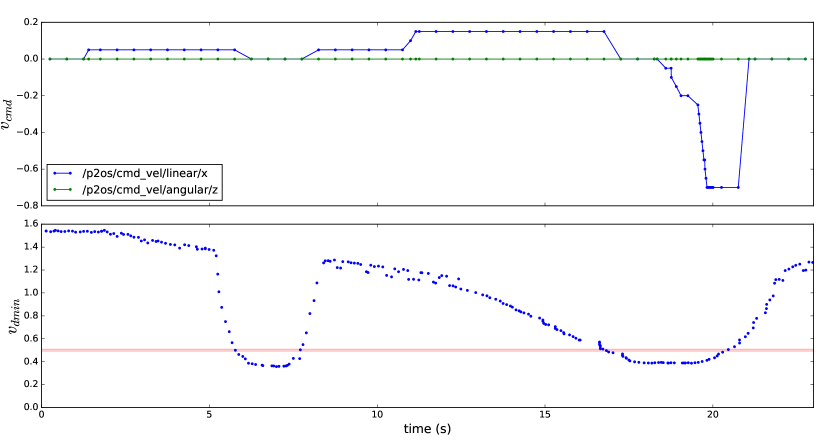
Figure 9: Visualization of an application run in the scenario. Plots (from top to bottom): (1) speed commands (linear and angular velocity) from the notebook, (2) minimum distance to an obstacle $v_{dmin}$ (based on LIDAR data) - the red area indicates the collision avoidance threshold.

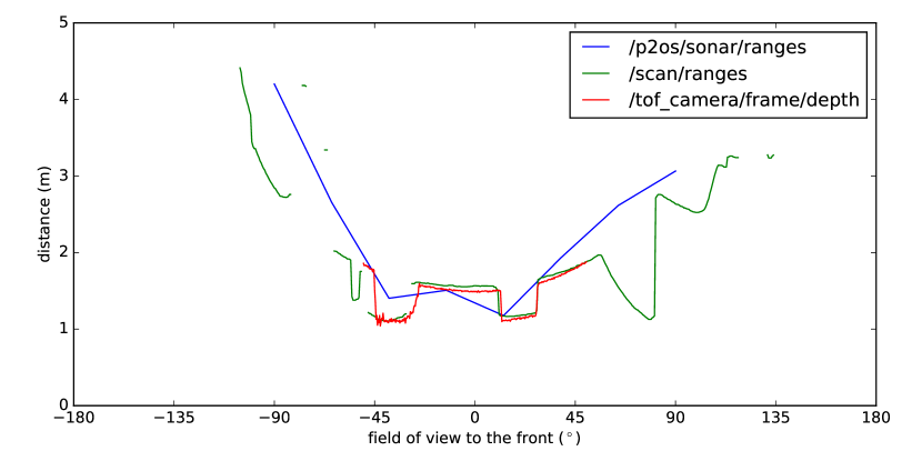
Figure 10: Signals in the domain $\mathsf{v}_{d\_2d}$ at about 7s. Observations of the sensors measuring distance to obstacles (sonar, LIDAR, ToF camera).

The distance measurements in Figure 10) show the significant differences, e.g., in field of view (the smallest is the one of the ToF camera) or resolution (8 measurements from the sonar vs. 320 from the ToF camera vs. 512 from the LIDAR), of the 3 sensors: sonar array, LIDAR and ToF camera. However, in the domain of $\mathsf{v}_{dmin}$ the observations can be reasonably compared though outliers have to be reckoned.

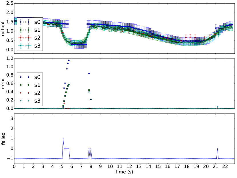
Figure 11: Monitor outputs over time of the demonstration. Plots (from top to bottom): (1) $\mathsf{v}_{dmin}$, outputs of the substitutions (executed by the monitor), (2) error per substitution (calculated by the monitor), (3) output status of the monitor – index of the failed substitution or -1 if all comparable substitution outputs match.

Figure 11 runs the monitor on the itoms collected above. The monitor triggers some faults due to improper timestamps of the sonar array (late when obstacle appears, but too early when the obstacle disappears) and an outlier of the same.

6.3 Fault Detection

To visualize and test the fault detection we inject faults to a generated set of itoms The itoms per monitor step have equal value and slightly shifted timestamps.

Table 3 summarizes the types of faults, how these are injected and the expected output of the monitor. Note that transient faults (outliers) can be mitigated by the additionally provided moving-median or moving-average filter of the monitor output. We therefore focus on faults occurring over a longer period of time (or permanent faults) and turn the filters off for reasonable plots of the results. All faults are injected for a specific period of time $[t_{start},t_{end}]$. $k$ faults can be identified when the number of comparable outputs is $\geq 2k+1$ (for Byzantine faults: $3k+1$). To be able to identify a fault in our setup, we assume only one simultaneous fault in the value domain. The buffer size $n_{buf}$ of the monitor is set to 1 for testing faults in the value domain.

Fault	Injection
Random noise	Add noise sample $x\sim U(a,b)$ to the observation.
Stuck-at 0	Set observation to $0$.
Time shift	Add the duration $\Delta$ to the reception timestamp $t_{r}$ of the observation.
Missing or lost messages	Delay observations by $\Delta>n_{buf}\cdot T_{m}$ (implemented by time shift).

Table 3: Fault injection to an input signal of a substitution.

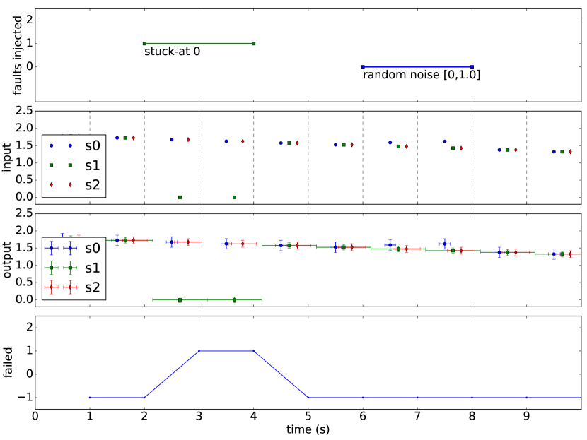
Figure 12: Fault detection in the value domain. From top to bottom: (1) reception of inputs (points) and monitor calls (dashed vertical lines), (2) outputs of the substitutions including uncertainty, (3) fault injection, (4) monitor output (index of the failed substitution or -1 if all substitution outputs match).

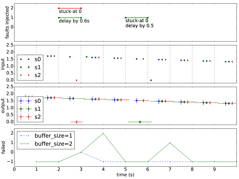
Figure 13: Fault detection in the time domain. From top to bottom: (1) fault injection, (2) reception of inputs (points) and monitor calls (dashed vertical lines), (3) outputs of the substitutions of the monitor $n_{buf}$=2, (4) monitor output (index of the failed substitution or -1 if all substitution outputs match).

Figures 12 and 13 visualizes fault detection of 3 substitution outputs. The top plot annotates the time span with a description of the injected fault. The height of the bar references the substitution index to which the fault has been injected. The generated value is represented by a marker while the uncertainty (intervals) is plotted as two error bars along the x- (time) and y-axis (value). The upper plot presents the timeline of reception of the monitor inputs ($t_{r}$ of the itoms). The lower plot shows the outputs of the substitution executed by the monitor, i.e., the itoms at the time of occurrence ($t_{s}$ or $\boldsymbol{t}$ of the itoms). The bottom indicates the substitution index with the highest error.

For instance, in Fig. 12 stuck-at 0 and random noise has been applied to the input of substitution $s_{1}$ and $s_{0}$, respectively. The monitor gathers the itoms since the last call (here within the last second) and compares the outputs of the substitutions when the time intervals overlap. Because the value intervals of $s_{1}$ during the time marked with “stuck-at 0” do not overlap the value intervals of the other substitutions $s_{1}$ has an error $\neq 0$ and the monitor indicates the failed substitution as $s_{1}$.

In Fig. 13 the capability to compensate delays is tested. The input of $s_{1}$ is missing in the monitor call at time $3s$. The faulty substitution is miss-classified because of only two available outputs to compare (no majority vote possible). However, with a buffer size of $n_{buf}=2$ the fault can be detected (the monitor collects itoms within $n_{buf}\cdot T_{m}$, here, the last 2 monitor periods). The delayed itom of $s_{1}$ can be compared to the itoms of the last call. It matches the output of $s_{0}$, so the monitor classifys $s_{2}$ as faulty at time $4s$.

The logged data and the scripts to inject faults and run the monitor offline can be found on GitHub .

7 Conclusion

A cyber-physical system (CPS) assembled out of many sub-systems provides observations of different CPS variables which can be interrelated to each other in a knowledge base. We present a monitor querying the knowledge base to find redundancies and which can detect faults of observation components by comparison. The knowledge base has been encoded in Prolog implemented with the ProbLog library which enables the user to change the knowledge base during runtime, and add or remove information about the availability of observations. The monitor can therefore master technological or functional changes in the CPS. Moreover, we presented an observation model considering uncertainties in space and time (e.g., noise or delays) of observations collected by the monitor.

In ongoing and future work we want to investigate other methods to compare and rank the redundant observations over time. Furthermore, we look into how the redundancy shall be selected (diversity) or proper fault diagnosis can be applied.

References

- [1] Varun Chandola, Arindam Banerjee, and Vipin Kumar. Anomaly Detection: A Survey. ACM Comput. Surv., 41(3):15:1–15:58, July 2009.
- [2] I. Butun, S. D. Morgera, and R. Sankar. A Survey of Intrusion Detection Systems in Wireless Sensor Networks. IEEE Communications Surveys Tutorials, 16(1):266–282, First 2014.
- [3] Robert Mitchell and Ing-Ray Chen. A Survey of Intrusion Detection Techniques for Cyber-physical Systems. ACM Comput. Surv., 46(4):55:1–55:29, March 2014.
- [4] A. L. Buczak and E. Guven. A Survey of Data Mining and Machine Learning Methods for Cyber Security Intrusion Detection. IEEE Communications Surveys Tutorials, 18(2):1153–1176, Secondquarter 2016.
- [5] Ezio Bartocci and Yliès Falcone, editors. Lectures on Runtime Verification: Introductory and Advanced Topics. Programming and Software Engineering. Springer International Publishing, 2018.
- [6] Yliès Falcone, Leonardo Mariani, Antoine Rollet, and Saikat Saha. Runtime Failure Prevention and Reaction. In Lectures on Runtime Verification, volume 10457 of Lecture Notes in Computer Science, pages 103–134. Springer, February 2018.
- [7] R. E. Kalman. A New Approach to Linear Filtering and Prediction Problems. Journal of Basic Engineering, 82(1):35–45, March 1960.
- [8] Maurice Bellanger and Maurice Bellanger. Adaptive digital filters. 2001.
- [9] Hermann Kopetz. Real-Time Systems: Design Principles for Distributed Embedded Applications. Springer, New York, 2nd edition, 2011.
- [10] Stefan Poledna. Fault-Tolerant Real-Time Systems: The Problem of Replica Determinism. Kluwer Academic Publishers, Norwell, MA, USA, 1996.
- [11] Oliver Höftberger. Knowledge-Based Dynamic Reconfiguration for Embedded Real-Time Systems. PhD thesis, TU Wien, Institute of Computer Engineering, Wien, 2015.
- [12] Tiago Amorim, Denise Ratasich, Georg Macher, Alejandra Ruiz, Daniel Schneider, Mario Driussi, and Radu Grosu. Runtime Safety Assurance for Adaptive Cyber-Physical Systems: ConSerts M and Ontology-Based Runtime Reconfiguration Applied to an Automotive Case Study. Solutions for Cyber-Physical Systems Ubiquity, pages 137–168, 2018.
- [13] D. Ratasich, T. Preindl, K. Selyunin, and R. Grosu. Self-healing by property-guided structural adaptation. In 2018 IEEE Industrial Cyber-Physical Systems (ICPS), pages 199–205, May 2018.
- [14] D. Ratasich, O. Höftberger, H. Isakovic, M. Shafique, and R. Grosu. A Self-Healing Framework for Building Resilient Cyber-Physical Systems. In 2017 IEEE 20th International Symposium on Real-Time Distributed Computing (ISORC), pages 133–140, May 2017.
- [15] S. Papa, W. Casper, and S. Nair. A transfer function based intrusion detection system for SCADA systems. In 2012 IEEE Conference on Technologies for Homeland Security (HST), pages 93–98, November 2012.
- [16] S. Ntalampiras. Detection of Integrity Attacks in Cyber-Physical Critical Infrastructures Using Ensemble Modeling. IEEE Transactions on Industrial Informatics, 11(1):104–111, February 2015.
- [17] H. Zhang, Q. Zhang, J. Liu, and H. Guo. Fault Detection and Repairing for Intelligent Connected Vehicles Based on Dynamic Bayesian Network Model. IEEE Internet of Things Journal, 5(4):2431–2440, August 2018.
- [18] Algirdas Avizienis, Jean-Claude Laprie, Brian Randell, and Carl Landwehr. Basic Concepts and Taxonomy of Dependable and Secure Computing. IEEE Trans. on Dependable and Secure Computing, 1(1):11–33, 2004.
- [19] S. Siva Sathya and K. Syam Babu. Survey of fault tolerant techniques for grid. Computer Science Review, 4(2):101 – 120, 2010.
- [20] Thomas Herault and Yves Robert, editors. Fault-Tolerance Techniques for High-Performance Computing. Computer Communications and Networks. Springer International Publishing, 2015.
- [21] Debanjan Ghosh, Raj Sharman, H. Raghav Rao, and Shambhu Upadhyaya. Self-healing systems — survey and synthesis. Decision Support Systems, 42(4):2164–2185, January 2007.
- [22] Harald Psaier and Schahram Dustdar. A survey on self-healing systems: Approaches and systems. Computing, 91(1):43–73, January 2011.
- [23] Jürgen Dürrwang, Marcel Rumez, Johannes Braun, and Reiner Kriesten. Security Hardening with Plausibility Checks for Automotive ECUs. In VEHICULAR 2017: The Sixth International Conference on Advances in Vehicular Systems, Technologies and Applications, pages 38–41. IARIA, July 2017.
- [24] Wilfried Elmenreich. Fusion of Continuous-valued Sensor Measurements using Confidence-weighted Averaging. Journal of Vibration and Control, 13(9-10):1303–1312, September 2007.
- [25] H. Zhang, J. Liu, and N. Kato. Threshold Tuning-Based Wearable Sensor Fault Detection for Reliable Medical Monitoring Using Bayesian Network Model. IEEE Systems Journal, 12(2):1886–1896, June 2018.
- [26] Morgan Quigley, Ken Conley, Brian Gerkey, Josh Faust, Tully Foote, Jeremy Leibs, Rob Wheeler, and Andrew Y. Ng. ROS: An open-source Robot Operating System. In ICRA Workshop on Open Source Software, volume 3, page 5. Kobe, Japan, 2009.
- [27] Hermann Kopetz. A Conceptual Model for the Information Transfer in Systems-of-Systems. In 2014 IEEE 17th International Symposium on Object/Component/Service-Oriented Real-Time Distributed Computing, pages 17–24, June 2014.
- [28] Anton Dries, Angelika Kimmig, Wannes Meert, Joris Renkens, Guy Van den Broeck, Jonas Vlasselaer, and Luc De Raedt. ProbLog2: Probabilistic Logic Programming. In Albert Bifet, Michael May, Bianca Zadrozny, Ricard Gavalda, Dino Pedreschi, Francesco Bonchi, Jaime Cardoso, and Myra Spiliopoulou, editors, Machine Learning and Knowledge Discovery in Databases, Lecture Notes in Computer Science, pages 312–315. Springer International Publishing, 2015.
- [29] Jean-Pierre Richard. Time-delay systems: An overview of some recent advances and open problems. Automatica, 39(10):1667–1694, October 2003.
- [30] Rupak Majumdar and Vinayak S. Prabhu. Computing the Skorokhod Distance Between Polygonal Traces. In Proceedings of the 18th International Conference on Hybrid Systems: Computation and Control, HSCC ’15, pages 199–208, New York, NY, USA, 2015. ACM.
- [31] T. Hickey, Q. Ju, and M. H. Van Emden. Interval arithmetic: From principles to implementation. Journal of the ACM (JACM), 48(5):1038–1068, January 2001.