Structured Knowledge Distillation for
Dense Prediction

Abstract

In this work, we consider transferring the structure information from large networks to compact ones for dense prediction tasks in computer vision. Previous knowledge distillation strategies used for dense prediction tasks often directly borrow the distillation scheme for image classification and perform knowledge distillation for each pixel separately, leading to sub-optimal performance. Here we propose to distill structured knowledge from large networks to compact networks, taking into account the fact that dense prediction is a structured prediction problem. Specifically, we study two structured distillation schemes: i) pair-wise distillation that distills the pair-wise similarities by building a static graph; and ii) holistic distillation that uses adversarial training to distill holistic knowledge. The effectiveness of our knowledge distillation approaches is demonstrated by experiments on three dense prediction tasks: semantic segmentation, depth estimation and object detection. Code is available at: https://git.io/StructKD

1 Introduction

Dense prediction is a family of fundamental problems in computer vision, which learns a mapping from input images to complex output structures, including semantic segmentation, depth estimation and object detection, among many others. One needs to assign category labels or regress specific values for each pixel given an input image to form the structured outputs. In general these tasks are significantly more challenging to solve than image-level prediction problems, thus often requiring networks with large capacity in order to achieve satisfactory accuracy. On the other hand, compact models are desirable for enabling computing on edge devices with limited computation resources.

Deep neural networks have been the dominant solutions since the invention of fully-convolutional neural networks (FCNs) [1]. Subsequent approaches, e.g., DeepLab [2], PSPNet [3], RefineNet [4], and FCOS [5] follow the design of FCNs to optimize energy-based objective functions related to different tasks, having achieved significant improvement in accuracy, often with cumbersome models and expensive computation.

Recently, design of neural networks with compact model sizes, light computation cost and high performance, has attracted much attention due to the need of applications on mobile devices. Most current efforts have been devoted to designing lightweight networks specifically for dense prediction tasks or borrowing the design from classification networks, e.g., ENet [6], ESPNet [6] and ICNet [7] for semantic segmentation, YOLO [8] and SSD [9] for object detection, and FastDepth [10] for depth estimation. Strategies such as pruning [10], knowledge distillation [11, 12] are applied to helping the training of compact networks by making use of cumbersome networks.

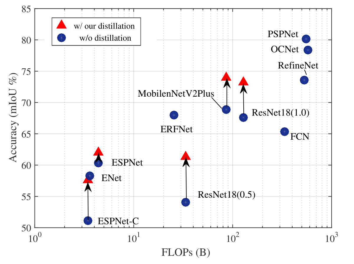
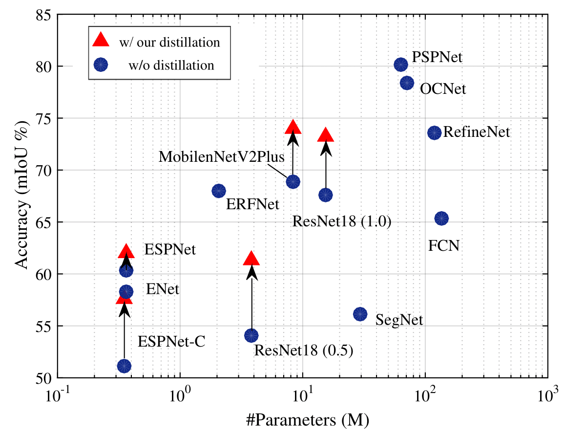
Figure 1: An example on the semantic segmentation task shows comparisons in terms of computation complexity, number of parameters and mIoU for different networks on the Cityscapes test set. The FLOPs is calculated with the input resolution of $512\times 1024$ pixels. Red triangles are the results of our distillation method while others are without distillation. Blue circles are collected from FCN* [1], RefineNet [4], SegNet [13], ENet [6], PSPNet [3], ERFNet [14], ESPNet [15], MobileNetV2Plus [16], and OCNet [17]. With our proposed distillation method, we can achieve a higher mIoU, with no extra FLOPs and parameters.

Knowledge distillation has proven effective in training compact models for classification tasks [18, 19]. As for dense prediction tasks, most previous works [11, 12] directly apply distillation at each pixel separately to transfer the class probability from the cumbersome network (teacher) to the compact network (student); or to extract more discriminative feature embeddings for the compact network. Note that, such a pixel-wise distillation scheme neglects the important structure information.

Considering the characteristic of dense prediction problem, here we present structured knowledge distillation and transfer the structure information with two schemes, pair-wise distillation and holistic distillation. The pair-wise distillation scheme is motivated by the widely-studied pair-wise Markov random field framework [20] for enforcing spatial labeling consistency. The goal is to align a static affinity graph which is computed to capture both short and long range structure information among different locations from the compact network and the teacher network.

The holistic distillation scheme aims to align higher-order consistencies, which are not characterized in the pixel-wise and pair-wise distillation, between output structures produced from the compact network and the teacher network. We adopt the adversarial training scheme, and a fully convolutional network, a.k.a. the discriminator, considering both the input image and the output structures to produce a holistic embedding which represents the quality of the structure. The compact network is encouraged to generate structures with similar embeddings as the teacher network. We encode the structure knowledge into the weights of discriminators.

To this end, we optimize an objective function that combines a conventional task loss with the distillation terms. The main contributions of this paper are as follows.

• We study the knowledge distillation strategy for training accurate compact networks for dense prediction.

• We present two structured knowledge distillation schemes, pair-wise distillation and holistic distillation, enforcing pair-wise and high-order consistency between the outputs of the compact and teacher networks.

• We demonstrate the effectiveness of our approach by improving recent state-of-the-art compact networks on three different dense prediction tasks: semantic segmentation, depth estimation and object detection. Taking semantic segmentation as an example, the performance gain is illustrated in Figure  1.

1.1 Related Work

Semantic segmentation. Semantic segmentation is a pixel classification problem, which requires an semantic understanding of the whole scene. Deep convolutional neural networks have been the dominant solution to semantic segmentation since the pioneering work, fully-convolutional network [1]. Various schemes have been developed for improving the network capability and accordingly the segmentation performance. For example, stronger backbone networks such as ResNet [21], DenseNet [22] and HRNet [SunXLW19, hrnet], have shown improved segmentation performance. Retaining the spatial resolution through dilated convolutions [2] or multi-path refine networks [4] leads to significant performance gain. Exploiting multi-scale context using dilated convolutions [23], or pyramid pooling modules as in PSPNet [3], also benefits the segmentation. Lin et al.  [24] combine deep models with structured output learning for semantic segmentation.

Recently, highly efficient segmentation networks have been attracting increasingly more interests due to the need of real-time and mobile applications. Most works focus on lightweight network design by accelerating the convolution operations with techniques such as factorization techniques. ENet [6], inspired by [25], integrates several acceleration factors, including multi-branch modules, early feature map resolution down-sampling, small decoder size, filter tensor factorization, and so on. SQ [26] adopts the SqueezeNet [27] fire modules and parallel dilated convolution layers for efficient segmentation. ESPNet [15] proposes an efficient spatial pyramid, which is based on filter factorization techniques: point-wise convolutions and spatial pyramid of dilated convolutions, to replace the standard convolution. The efficient classification networks such as MobileNet [28] and ShuffleNet [29] are also applied to accelerate segmentation. In addition, ICNet (image cascade network) [7] exploits the efficiency of processing low-resolution images and high inference quality of high-resolution ones, achieving a trade-off between efficiency and accuracy.

Depth estimation. Depth estimation from a monocular image is essentially an ill-posed problem, which requires an expressive model with large capacity. Previous works depend on hand-crafted features [30]. Since Eigen et al.  [31] propose to use deep learning to predict depth maps, following works [32, 33, 34, 35] benefit from the increasing capacity of deep models and achieve good results. Besides, Fei [36] propose a semantically informed geometric loss while Yin et al. [37] introduce a virtual normal loss to exploit geometric information. As in semantic segmentation, some works try to replace the encoder with efficient backbones [37, 38, 10] to decrease the computational cost, but often suffer from the limitation caused by the capacity of a compact network. The close work to ours [10] applies pruning to train the compact depth network. However, here we focus on the structured knowledge distillation.

Object detection. Object detection is a fundamental task in computer vision, in which one needs to regress the location of bounding boxes and predict a category label for each instance of interest in an image. Early works [39, 40] achieve good performance by first predicting proposals and then refining the localization of bounding boxes. Effort is also spent on improving detection efficiency with methods such as Yolo [8], and SSD [9]. They use a one-stage method and design light-weight network structures. RetinaNet [41] solves the problem of unbalance samples to some extent by proposing the focal loss, which makes the results of one-stage methods comparable to two-stage ones. Most of the above detectors rely on a set of pre-defined anchor boxes, which decreases the training samples and makes the detection network sensitive to hyper parameters. Recently, anchor free methods show promises, e.g., FCOS [5]. FCOS employs a fully convolutional framework, and predicts bounding box based on every pixels same as in semantic segmentation, which solves the object detection task as a dense prediction problem. In this work, we apply the structured knowledge distillation method with the FCOS framework, as it is simple and achieves promising performance.

Knowledge distillation. Knowledge distillation [18] transfers knowledge from a cumbersome model to a compact model so as to improve the performance of compact networks. It has been applied to image classification by using the class probabilities produced from the cumbersome model as “soft targets” for training the compact model [42, 18, 43] or transferring the intermediate feature maps [19, 44].

The MIMIC [11] method distills a compact object detection network by making use of a two-stage Faster-RCNN [40]. They align the feature map at the pixel level and do not make use of the structure information among pixels.

The recent and independent work, which applies distillation to semantic segmentation [12], is related to our approach. It mainly distills the class probabilities for each pixel separately (as our pixel-wise distillation) and center-surrounding differences of labels for each local patch (termed as a local relation in [12]). In contrast, we focus on distilling structured knowledge: pair-wise distillation, which transfers the relation among different locations by building a static affinity graph, and holistic distillation, which transfers the holistic knowledge that captures high-order information. Thus the work of [12] may be seen as a special case of the pair-wise distillation.

This work here is a substantial extension of our previous work appeared in [45]. The main difference compared with  [45] is threefold. 1) We extend the pair-wise distillation to a more general case in Section 2.1 and build a static graph with nodes and connections. We explore the influence of the graph size, and find out that it is important to keep a fully connected graph. 2) We provide more explanations and ablations on the adversarial training for holistic distillation. 3) We also extend our method to depth estimation and object detection with two recent strong baselines [37] and [5], by replacing the backbone with MobileNetV2 [46], and further improve their performance.

Adversarial learning. Generative adversarial networks (GANs) have been widely studied in text generation [47, 48] and image synthesis [49, 50]. The conditional version [51] is successfully applied to image-to-image translation, such as style transfer [52] and image coloring [53].

The idea of adversarial learning is also employed in pose estimation [54], encouraging the human pose estimation result not to be distinguished from the ground-truth; and semantic segmentation [55], encouraging the estimated segmentation map not to be distinguished from the ground-truth map. One challenge in [55] is the mismatch between the generator’s continuous output and the discrete true labels, making the discriminator in GAN be of very limited success. Different from [55], in our approach, the employed GAN does not face this issue as the ground truth for the discriminator is the teacher network’s logits, which are real valued. We use adversarial learning to encourage the alignment between the output maps produced from the cumbersome network and the compact network. However, in the depth prediction task, the ground truth maps are not discrete labels. In [56], the authors use the ground truth maps as the real samples. Different from theirs, our distillation methods attempt to align the output of the cumbersome network and that of the compact network. The task loss calculated with ground truth is optional. When the labelled data is limited, given a well-trained teacher, our method can be applied to unlabelled data and may further improve the accuracy.

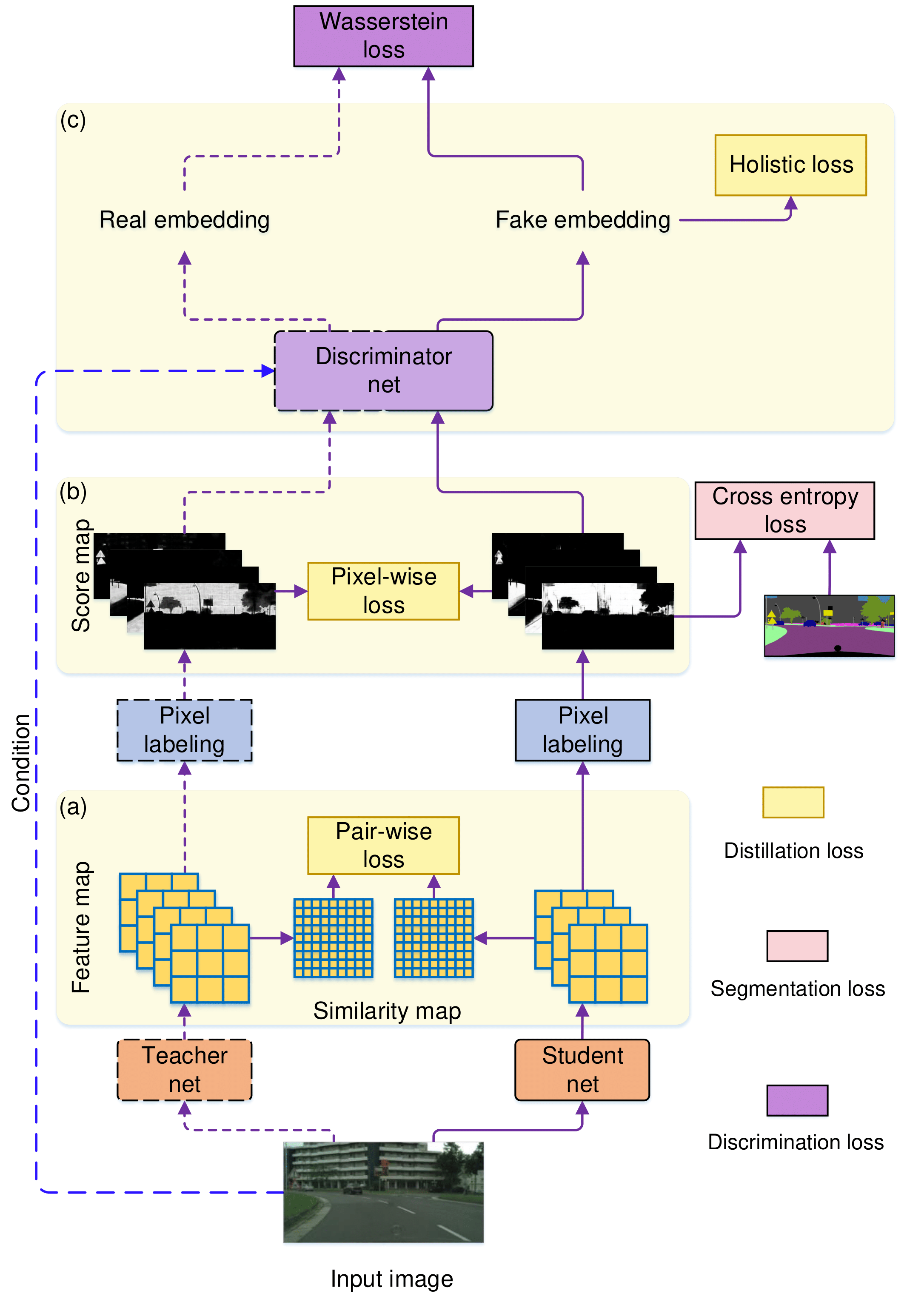
Figure 2: Our distillation framework with the semantic segmentation task as an example. (a) Pair-wise distillation; (b) Pixel-wise distillation; (c) Holistic distillation. In the training process, we keep the cumbersome network fixed as our teacher net, and only the student net and the discriminator net are optimized. The student net with a compact architecture is trained with the three distillation terms and a task-specific loss, e.g., the cross entropy loss for semantic segmentation.

2 Approach

In this section, we first introduce the structured knowledge distillation method for semantic segmentation, a task of assigning a category label to each pixel in the image from $C$ categories. A segmentation network takes a RGB image $\mathbf{I}$ of size $W\times H\times 3$ as the input; then it computes a feature map $\mathbf{F}$ of size $W^{\prime}\times H^{\prime}\times N$, where $N$ is the number of channels. Then, a classifier is applied to compute the segmentation map $\mathbf{Q}$ of size $W^{\prime}\times H^{\prime}\times C$ from $\mathbf{F}$, which is upsampled to the spatial size $W\times H$ of the input image to obtain the segmentation results. We extend our method to other two dense prediction tasks: depth estimation and object detection.

Pixel-wise distillation. We apply the knowledge distillation strategy [18] to transfer the knowledge of the large teacher segmentation network $\mathsf{T}$ to a compact segmentation network $\mathsf{S}$ for better training the compact segmentation network. We view the segmentation problem as a collection of separate pixel labeling problems, and directly use knowledge distillation to align the class probability of each pixel produced from the compact network. We follow [18] and use the class probabilities produced from the teacher model as soft targets for training the compact network.

The loss function is as follows,

$$\ell_{pi}(\mathsf{S})=\frac{1}{W^{\prime}\times H^{\prime}}\sum_{i\in\mathcal{R}}\operatorname{KL}(\mathbf{q}^{s}_{i}\|\mathbf{q}^{t}_{i}),$$ (1)

where $\mathbf{q}^{s}_{i}$ represents the class probabilities of the $i$th pixel produced from the compact network $\mathsf{S}$. $\mathbf{q}^{t}_{i}$ represents the class probabilities of the $i$th pixel produced from the cumbersome network $\mathsf{T}$. $\operatorname{KL}(\cdot)$ is the Kullback-Leibler divergence between two probabilities, and $\mathcal{R}=\{1,2,\dots,W^{\prime}\times H^{\prime}\}$ denotes all the pixels.

2.1 Structured Knowledge Distillation

In addition to above straightforward pixel-wise distillation, we present two structured knowledge distillation schemes—pair-wise distillation and holistic distillation—to transfer structured knowledge from the teacher network to the compact network. The pipeline is illustrated in Figure 2.

Pair-wise distillation. Inspired by the pair-wise Markov random field framework that is widely adopted for improving spatial labeling contiguity, we propose to transfer the pair-wise relations, specifically pair-wise similarities in our approach, among spatial locations.

We build an affinity graph to denote the spatial pair-wise relations, in which, the nodes represent different spatial locations and the connection between two nodes represents the similarity. We denote the connection range $\alpha$ and the granularity $\beta$ of each node to control the size of the static affinity graph. For each node, we only consider similarities with top-$\alpha$ near nodes according to spatial distance (here we use the Chebyshev distance) and aggregate $\beta$ pixels in a spatial local patch to represent the feature of this node as illustrate in Figure 3. Here for a $W^{\prime}\times H^{\prime}\times C$ feature map, $W^{\prime}\times H^{\prime}$ is the spatial resolution. With the granularity $\beta$ and the connection range $\alpha$, the affinity graph contains $\frac{W^{\prime}\times H^{\prime}}{\beta}$ nodes with $\frac{W^{\prime}\times H^{\prime}}{\beta}\times\alpha$ connections.

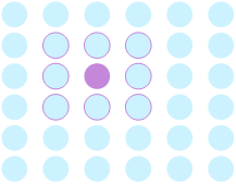
(a) $\alpha=9$, $\beta=1$

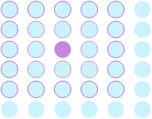
(b) $\alpha=25$, $\beta=1$

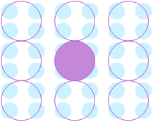
(c) $\alpha=9$, $\beta=4$

Figure 3: Illustrations of the connection range $\alpha$ and the granularity $\beta$ of each node.

Let $a^{t}_{ij}$ and $a^{s}_{ij}$ denote the similarity between the $i$th node and the $j$th node produced from the teacher network $\mathsf{T}$ and the compact network $\mathsf{S}$, respectively. We adopt the squared difference to formulate the pair-wise similarity distillation loss,

$$\ell_{pa}(\mathsf{S})=\frac{\beta}{W^{\prime}\times H^{\prime}\times\alpha}\sum_{i\in\mathcal{R^{\prime}}}\sum_{j\in\alpha}(a^{s}_{ij}-a^{t}_{ij})^{2}.$$ (2)

where $\mathcal{R^{\prime}}=\{1,2,\dots,\frac{W^{\prime}\times H^{\prime}}{\beta}\}$ denotes all the nodes. In our implementation, we use average pooling to aggregate $\beta\times C$ features in one node to be $1\times C$, and the similarity between two nodes is computed from the aggregated features $\mathbf{f}_{i}$ and $\mathbf{f}_{j}$ as

$$a_{ij}={\mathbf{f}_{i}^{\top}\mathbf{f}_{j}}/{(\|\mathbf{f}_{i}\|_{2}\|\mathbf{f}_{j}\|_{2})},$$

which empirically works well.

Holistic distillation. We align high-order relations between the segmentation maps produced from the teacher and compact networks. The holistic embeddings of the segmentation maps are computed as the representations.

We use conditional generative adversarial learning [51] for formulating the holistic distillation problem. The compact net is viewed as a generator conditioned on the input RGB image $\mathbf{I}$, and the predicted segmentation map $\mathbf{Q}^{s}$ is seen as a fake sample. The segmentation map predicted by the teacher ( $\mathbf{Q}^{t}$) is the real sample. We expect that $\mathbf{Q}^{s}$ is similar to $\mathbf{Q}^{t}$. Generative adversarial networks (GANs) usually suffer from the unstable gradient in training the generator due to the non-smoothness of the discontinuous Kullback–Leibler (KL) or Jensen-Shannon (JS) divergence when the two distributions do not overlap. The Wasserstein distance [57] provides a smooth measure of the difference between two distributions. The Wasserstein distance is defined as the minimum cost to converge the model distribution $p_{s}(\mathbf{Q}^{s})$ to the real distribution $p_{t}(\mathbf{Q}^{t})$. This can be written as follows:

$$\ell_{ho}(\mathsf{S},\mathsf{D})= ~{}\mathbb{E}_{\mathbf{Q}^{s}\sim p_{s}(\mathbf{Q}^{s})}[\mathsf{D}(\mathbf{Q}^{s}|\mathbf{I})]-\mathbb{E}_{\mathbf{Q}^{t}\sim p_{t}(\mathbf{Q}^{t})}[\mathsf{D}(\mathbf{Q}^{t}|\mathbf{I})],$$ (3)

where $\mathbb{E}[\cdot]$ is the expectation operator, and $\mathsf{D}(\cdot)$ is an embedding network, acting as the discriminator in GAN, which projects $\mathbf{Q}$ and $\mathbf{I}$ together into a holistic embedding score. The Lipschitz constraint is enforced by applying a gradient penalty [57].

The segmentation map and the RGB image are concatenated as the input of the embedding network $\mathsf{D}$. $\mathsf{D}$ is a fully convolutional neural network with five convolution blocks. Each convolution block has ReLU and BN layers, except for the final output convolution block. Two self-attention modules are inserted between the final three blocks to capture the structure information [58]. We insert a batch normalization immediately after the input so as to normalize the scale difference between the segmentation map and RGB channels.

Such a discriminator is able to produce a holistic embedding representing how well the input image and the segmentation map match. We further add a pooling layer to pool the holistic embedding into a score. As we employ the Wasserstein distance in the adversarial training, the discriminator is trained to produce a higher score w.r.t. the output segmentation map from the teacher net and produce lower scores w.r.t. the ones from the student. In this process, we encode the knowledge of evaluating the quality of a segmentation map into the discriminator. The student is trained with the regularization of achieving a higher score under the evaluation of the discriminator, thus improving the performance of the student.

2.2 Optimization

The overall objective function consists of a standard multi-class cross-entropy loss $\ell_{mc}(\mathsf{S})$ with pixel-wise and structured distillation terms

$$\ell(\mathsf{S},\mathsf{D})= ~{}\ell_{mc}(\mathsf{S})+\lambda_{1}(\ell_{pi}(\mathsf{S})+\ell_{pa}(\mathsf{S}))-\lambda_{2}\ell_{ho}(\mathsf{S},\mathsf{D}),$$ (4)

where $\lambda_{1}$ and $\lambda_{2}$ are set to $10$ and $0.1$, making these loss value ranges comparable. We minimize the objective function with respect to the parameters of the compact segmentation network $\mathsf{S}$, while maximizing it w.r.t. the parameters of the discriminator $\mathsf{D}$, which is implemented by iterating the following two steps:

• Train the discriminator $\mathsf{D}$. Training the discriminator is equivalent to minimizing $\ell_{ho}(\mathsf{S},\mathsf{D})$. $\mathsf{D}$ aims to give a high embedding score for the real samples from the teacher net and low embedding scores for the fake samples from the student net.

• Train the compact segmentation network $\mathsf{S}$. Given the discriminator network, the goal is to minimize the multi-class cross-entropy loss and the distillation losses relevant to the compact segmentation network:

  $$\ell_{mc}(\mathsf{S})+\lambda_{1}(\ell_{pi}(\mathsf{S})+\ell_{pa}(\mathsf{S}))-\lambda_{2}\ell^{s}_{ho}(\mathsf{S}),$$

  where

  $$\ell^{s}_{ho}(\mathsf{S})=\mathbb{E}_{\mathbf{Q}^{s}\sim p_{s}(\mathbf{Q}^{s})}[\mathsf{D}(\mathbf{Q}^{s}|\mathbf{I})]$$

  is a part of $\ell_{ho}(\mathsf{S},\mathsf{D})$ given in Equation (3), and we expect $\mathsf{S}$ to achieve a higher score under the evaluation of $\mathsf{D}$.

2.3 Extension to Other Dense Prediction Tasks

Dense prediction learns a mapping from an input RGB image $\mathbf{I}$ of size $W\times H\times 3$ to a per-pixel output $\mathbf{Q}$ of size $W\times H\times C$. In semantic segmentation, the output has $C$ channels which is the number of semantic classes.

For the object detection task, for each pixel, we predict the $c^{*}$ classes, as well as a 4D vector $t^{*}=(l,t,r,b)$ representing the location of a bounding box. We follow FCOS [5], and combine them with distillation terms as regularization.

The depth estimation task can be solved as a classification task, as the continuous depth values can be divided into $C$ discrete categories [59]. For inference, we apply a soft weighted sum as in [37]. The pair-wise distillation can be directly applied to the intermediate feature maps. The holistic distillation uses the depth map as input. We can use the ground truth as the real samples of GAN in the depth estimation task, because it is a continuous map. However, in order to apply our method to unlabelled data, we still use depth maps from the teacher as our real samples.

3 Experiments

In this section, we first apply our method to semantic segmentation to empirically verify the effectiveness of structured knowledge distillation. We discuss and explore how structured knowledge distillation works.

Structured knowledge distillation can be applied to other structured output prediction tasks with FCN frameworks. In Section 3.3 and Section 3.2, we apply our distillation method to strong baselines in object detection and depth estimation tasks with minimum modifications.

3.1 Semantic Segmentation

3.1.1 Implementation Details

Network structures. We use the segmentation architecture of PSPNet [3] with a ResNet$101$ [21] as the teacher network $\mathsf{T}$.

We study recent compact networks, and employ several different architectures to verify the effectiveness of the distillation framework. We first use ResNet$18$ as a basic student network and conduct ablation studies. Then, we employ the MobileNetV$2$Plus [16], which is based on a pretrained MobileNetV$2$ [46] model on the ImageNet dataset. We also test ESPNet-C [15] and ESPNet [15] models, which are also lightweight models.

Training setup. Unless otherwise specified, segmentation networks here using stochastic gradient descent (SGD) with the momentum ($0.9$) and the weight decay ($0.0005$) for $40000$ iterations. The learning rate is initialized to be $0.01$ and is multiplied by $(1-\frac{iter}{max-iter})^{0.9}$. We random crop the images into the resolution of $512\times 512$ pixels as the training input. Standard data augmentation is applied during training, such as random scaling (from $0.5$ to $2.1$) and random flipping. We follow the settings in [15] to reproduce the results of ESPNet and ESPNet-C, and train the compact networks with our distillation framework.

3.1.2 Datasets

Cityscapes. The Cityscapes dataset [60] is collected for urban scene understanding and contains $30$ classes with only $19$ classes used for evaluation. The dataset contains $5,000$ high quality finely annotated images and $20,000$ coarsely annotated images. The finely annotated images are divided into $2,975$, $500$, $1,525$ images for training, validation and testing. We only use the finely annotated dataset in our experiments.

CamVid. The CamVid dataset [61] contains $367$ training and $233$ testing images. We evaluate the performance over $11$ different classes such as building, tree, sky, car, road, etc.

ADE$20$K. The ADE$20$K dataset [62] contains $150$ classes of diverse scenes. The dataset is divided into $20K$/$2K$/$3K$ images for training, validation and testing.

3.1.3 Evaluation Metrics

We use the following metrics to evaluate the segmentation accuracy, model size and the efficiency.

The Intersection over Union (IoU) score is calculated as the ratio of interval and union between the ground-truth mask and the predicted segmentation mask for each class. We use the mean IoU of all classes (mIoU) to study the effectiveness of distillation. We also report the class IoU to study the effect of distillation on different classes. Pixel accuracy is the ratio of the pixels with the correct semantic labels to the overall pixels.

The model size is represented by the number of network parameters. and the complexity is evaluated by the sum of floating point operations (FLOPs) in one forward on a fixed input size.

3.1.4 Ablation Study

The effectiveness of distillations. We examine the role of each component of our distillation system. The experiments are conducted on ResNet$18$ with its variant ResNet$18$ ($0.5$) representing a width-halved version of ResNet$18$ on the Cityscapes dataset. Table I reports the results of different settings for the student net, which are the average results of the final epoch from three runs.

TABLE I: The effect of different components of the loss in the proposed method. PI: pixel-wise distillation; PA: pair-wise distillation; HO: holistic distillation; ImN: initialized from the pretrain weight on the ImageNet.

Method	Validation mIoU (%)	Training mIoU (%)
Teacher	$78.56$	$86.09$
ResNet$18$ ($0.5$)	$55.37\pm 0.25$	$60.67\pm 0.37$
+ PI	$57.07\pm 0.69$	$62.33\pm 0.66$
+ PI + PA	$61.52\pm 0.09$	$66.03\pm 0.07$
+ PI + PA + HO	$\bf{62.35}\pm 0.12$	$\bf{66.72\pm 0.04}$
ResNet$18$ ($1.0$)	$57.50\pm 0.49$	$62.98\pm 0.45$
+ PI	$58.63\pm 0.31$	$64.32\pm 0.32$
+ PI + PA	$62.97\pm 0.06$	$68.97\pm 0.03$
+ PI + PA + HO	$\bf{64.68}\pm 0.11$	$\bf{70.04}\pm 0.06$
ResNet$18$ ($1.0$)	$69.10\pm 0.21$	$74.12\pm 0.19$
+ PI +ImN	$70.51\pm 0.37$	$75.10\pm 0.37$
+ PI + PA +ImN	$71.78\pm 0.03$	$77.66\pm 0.02$
+ PI + PA + HO +ImN	$\bf{74.08}\pm 0.13$	$\bf{78.75\pm 0.02}$

From Table I, we can see that distillation can improve the performance of the student network, and structure distillation helps the student learn better. With the three distillation terms, the improvements for ResNet$18$ ($0.5$), ResNet$18$ ($1.0$) and ResNet$18$ ($1.0$) initialized with pretrained weights on the ImageNet dataset are $6.26\%$, $5.74\%$ and $2.9\%$, respectively, which indicates that the effect of distillation is more pronounced for the smaller student network and networks without initialization with the weight pretrained from the ImageNet. Such an initialization is also able to transfer the knowledge from another source (ImageNet). The best mIoU of the holistic distillation for ResNet$18$ ($0.5$) reaches $62.7\%$ on the validation set.

On the other hand, each distillation scheme leads to higher mIoU scores. This implies that the three distillation schemes make complementary contributions for better training the compact network.

The affinity graph in pair-wise distillation. In this section, we discuss the impact of the connection range $\alpha$ and the granularity of each node $\beta$ in building the affinity graph. To calculate the pair-wise similarity among each pixel in the feature map will form the fully connected affinity graph, with the price of high computational complexity. We fix the node to be one pixel, and vary the connection range $\alpha$ from the fully connected graph to local sub-graph. Then, we keep the connection range $\alpha$ to be fully connected, and use a local patch to denote each node to change the granularity $\beta$ from fine to coarse. The result are shown in Table II. The results of different settings for the pair-wise distillation are the average results from three runs. We employ a ResNet$18$ ($1.0$) with the weight pretrained from ImageNet as the student network. All the experiments are performed with both pixel-wise distillation and pair-wise distillation, but the sizes of the affinity graph in pair-wise distillation vary.

From Table II, we can see that increasing the connection range can help improve the distillation performance. With the fully connected graph, the student can achieve around $71.37\%$ mIoU. It appears that the best $\beta$ is $2\times 2$, which is slightly better than the finest affinity graph, but the connections are significantly decreased. Using a small local patch to denote a node and calculate the affinity graph may form a more stable correlation between different locations. One can choose to use the local patch to decrease the number of the nodes, instead of decreasing the connection range for a better trade-off between efficiency and accuracy.

To include more structure information, we fuse pair-wise distillation items with different affinity graphs. Three pair-wise fusion strategies are introduced: $\alpha$ fusion, $\beta$ fusion and feature level fusion. The details are shown in Table II. We can see that combining more affinity graphs may improve the performance, but also introduces extra computational cost during training. Therefore, we apply only one pair-wise distillation item in our methods.

TABLE II: The impact of the connection range and node granularity. The shape of the output feature map is $H^{\prime}\times W^{\prime}$. We can see that to keep a fully connected graph is more helpful in pair-wise distillation.

Method	Validation mIoU(%)	Connections
Teacher	$78.56$	$-$
Resnet18 (1.0)	$69.10\pm 0.21$	$-$
$\beta=1\times 1$, $\alpha=$
$W^{\prime}/16\times H^{\prime}/16$	$70.83\pm 0.12$	$(W^{\prime}\times H^{\prime})^{2}/2^{8}$
$W^{\prime}/8\times H^{\prime}/8$	$70.94\pm 0.11$	$(W^{\prime}\times H^{\prime})^{2}/2^{6}$
$W^{\prime}/4\times H^{\prime}/4$	$71.09\pm 0.07$	$(W^{\prime}\times H^{\prime})^{2}/2^{4}$
$W^{\prime}/2\times H^{\prime}/2$	$71.15\pm 0.01$	$(W^{\prime}\times H^{\prime})^{2}/4$
$W\times H$	$71.37\pm 0.12$	$(W^{\prime}\times H^{\prime})^{2}$
$\alpha=W^{\prime}\times H^{\prime}/\beta$, $\beta=$
$2\times 2$	$\bf{71.78\pm 0.03}$	$(W^{\prime}\times H^{\prime})^{2}/2^{4}$
$4\times 4$	$71.24\pm 0.18$	$(W^{\prime}\times H^{\prime})^{2}/2^{8}$
$8\times 8$	$71.10\pm 0.36$	$(W^{\prime}\times H^{\prime})^{2}/2^{12}$
$16\times 16$	$71.11\pm 0.14$	$(W^{\prime}\times H^{\prime})^{2}/2^{16}$
$32\times 32$	$70.94\pm 0.23$	$(W^{\prime}\times H^{\prime})^{2}/2^{20}$
Multi-level pair-wise distillations
$\alpha$ Fusion1	$72.03\pm 0.26$	$21*(W^{\prime}\times H^{\prime})^{2}/2^{8}$
$\beta$ Fusion2	$71.91\pm 0.17$	$273*(W\times H)^{2}/2^{12}$
Feature-level Fusion3	$\bf{72.18\pm 0.12}$	$3*(W^{\prime}\times H^{\prime})^{2}/2^{4}$

• Different connection ranges fusion, with output feature size $H^{\prime}\times W^{\prime}$, $\beta=2\times 2$ and $\alpha$ as $W^{\prime}/2\times H^{\prime}/2$, $W^{\prime}/4\times H^{\prime}/4$ and $W^{\prime}/8\times H^{\prime}/8$, respectively.

• Different node granulates fusion, with output feature size $H^{\prime}\times W^{\prime}$, $\beta$ as $2\times 2$, $4\times 4$ and $8\times 8$, respectively, and $\alpha$ as $W^{\prime}\times H^{\prime}/\beta$.

• Different feature levels fusion, with feature size $H^{\prime}\times W^{\prime}$, $2H^{\prime}\times 2W^{\prime}$, $4H^{\prime}\times 4W^{\prime}$, $\beta$ as $2\times 2$, $4\times 4$ and $8\times 8$, respectively, and $\alpha$ as maximum.

Adversarial training in holistic distillation. In this section, we illustrate that GAN is able to encode the holistic knowledge. Details of the discriminator are described in Section 3. The capability of discriminator would affect the adversarial training, and we conduct experiments to discuss the impact of the discriminator’s architecture. The results are shown in Table III. We use $AnLm$ to represent the architecture of the discriminator with $n$ self-attention layers and $m$ convolution blocks with BN layers. The detailed structures can be seen in Figure 4, and the red arrows represent self-attention layers.

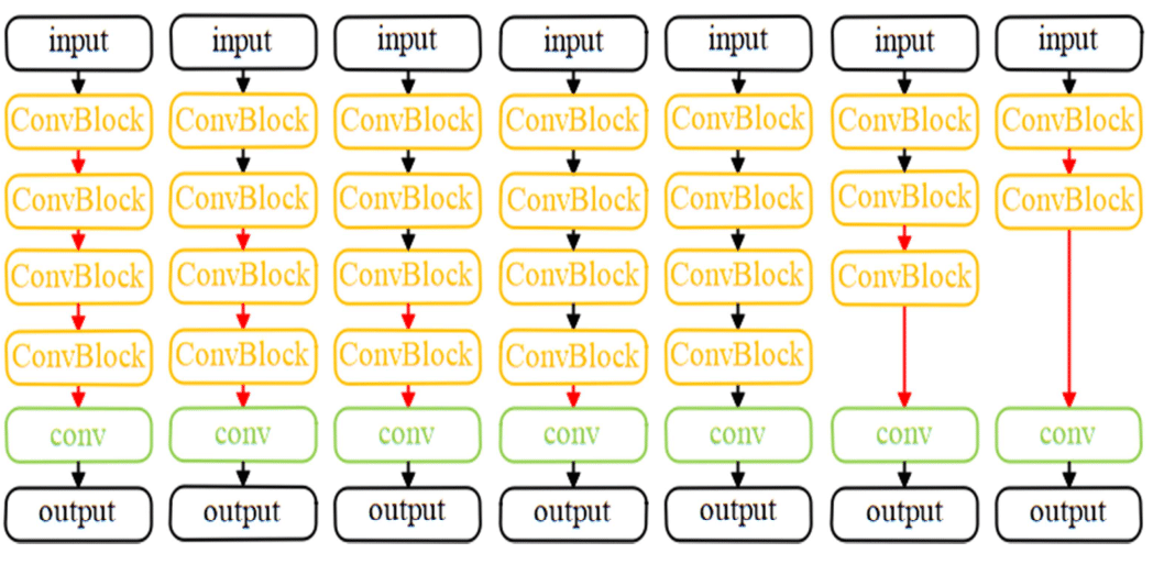
Figure 4: We show $7$ different architectures of the discriminator. The red arrow represents a self-attention layer. The orange block denotes a convolution block with stride $2$. We insert an average pooling layer to the output block to obtain the final score.

From Table III, we can see adding self-attention layers can improve mIoU, and adding more self-attention layers does not change the results much. We add $2$ self-attention blocks considering the performance, stability, and computational cost in our discriminator. With the same self-attention layer, a deeper discriminator can help the adversarial training.

TABLE III: We choose ResNet$18$ ($1.0$) as the example for the student net. An $AnLm$ index represents for $n$ self-attention layers with $m$ convolution blocks in the discriminator. The ability of discriminator affects the adversarial training.

Architecture Index	Validation mIoU (%)
Changing self-attention layers
A4L4	$73.46\pm 0.02$
A3L4	$73.70\pm 0.02$
A2L4 (ours)	$\bf{74.08\pm 0.13}$
A1L4	$74.05\pm 0.55$
A0L4	$72.85\pm 0.01$
Removing convolution blocks
A2L4 (ours)	$\bf{74.08\pm 0.13}$
A2L3	$73.35\pm 0.10$
A2L2	$72.24\pm 0.42$

TABLE IV: We choose ResNet$18$ ($1.0$) as the example for the student net. The numbers of class IoU with three different discriminator architectures are reported. Self-attention layers can significantly improve the accuracy of structured objects, such as truck, bus, train and motorcycle.

Class	mIoU	road	sidewalk	building	wall	fence	pole	Traffic light	Traffic sign	vegetation
D_Shallow	$72.28$	$97.31$	$80.07$	$91.08$	$36.86$	$50.93$	$62.13$	$66.4$	$76.77$	$91.73$
D_no_attention	$72.69$	$\bf{97.36}$	$\bf{80.22}$	$\bf{91.62}$	$\bf{45.16}$	$\bf{56.97}$	$62.23$	$\bf{68.09}$	$\bf{76.38}$	$\bf{91.94}$
D_Ours	$74.10$	$97.15$	$79.17$	$91.60$	$44.84$	$56.61$	$\bf{62.37}$	$67.37$	$76.34$	$91.91$
class	terrain	sky	person	rider	car	truck	bus	train	motorcycle	bicycle
D_Shallow	$60.14$	$93.76$	$79.89$	$55.32$	$93.45$	$69.44$	$73.83$	$69.54$	$48.98$	$75.78$
D_no_attention	$\bf{62.98}$	$\bf{93.84}$	$\bf{80.1}$	$\bf{57.35}$	$93.45$	$68.71$	$75.26$	$56.28$	$47.66$	$75.59$
D_Ours	$58.67$	$93.79$	$79.9$	$56.61$	$\bf{94.3}$	$\bf{75.83}$	$\bf{82.87}$	$\bf{72.03}$	$\bf{50.89}$	$\bf{75.72}$

To verify the effectiveness of adversarial training, we further explore the capability of three typical discriminators: the shallowest one (D_Shallow, i.e., A2L2), the one without attention layer (D_no_attention, i.e., A0L4) and ours (D_Ours, i.e., A2L4). The IoUs for different classes are listed in Table IV. It is clear that self-attention layers can help the discriminator better capture the structure, thus the accuracy of the students with the structure objects is improved.

In the adversarial training, the student, a.k.a.  the generator, tries to learn the distribution of the real samples (output of the teacher). We apply the Wasserstein distance to transfer the distance between two distributions into a more intuitive score, and the score are highly relevant to the quality of the segmentation maps. We use a well-trained discriminator $\mathsf{D}$ (A2L4) to evaluate the score of a segmentation map. For each image, we feed five segmentation maps, output by the teacher net, the student net w/o holistic distillation, and the student nets w/ holistic distillation under three different discriminator architectures (listed in Table IV) into the discriminator $\mathsf{D}$, and compare the distribution of embedding scores. We evaluate on the validation set and calculate the average score difference between different student nets and the teacher net, the results are shown in Table V. With holistic distillation, the segmentation maps produced from student net can achieve a similar score to the teacher, indicating that GAN helps distill the holistic structure knowledge.

TABLE V: We choose ResNet$18$ ($1.0$) as the example for the student net. The embedding score difference and mIoU on the validation set of Cityscapes are presented.

Method	Score difference	mIoU
Teacher	$0$	$78.56$
Student w/o D	$2.28$	$69.21$
w/ D_no_attention	$0.23$	$72.69$
w/ D_shallow	$0.46$	$72.28$
w/ D_ours	$0.14$	$74.10$

We also draw a histogram to show score distributions of segmentation maps across the validation set in Figure 5. The well-trained $\mathsf{D}$ can assign a higher score to high quality segmentation maps, and the three student nets with the holistic distillation can generate segmentation maps with higher scores and better quality. Adding self-attention layers and more convolution blocks help the student net to imitate the distribution of the teacher net, and attain better performance.

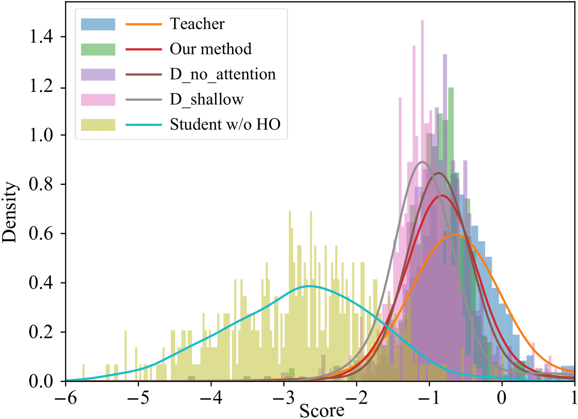
Figure 5: The score distribution of segmentation maps generated by different student nets evaluated by a well-trained discriminator. With adversarial training, score distributions of segmentation maps become closer to the teacher (the orange one); and our method (the red one) is the closest one to the teacher.

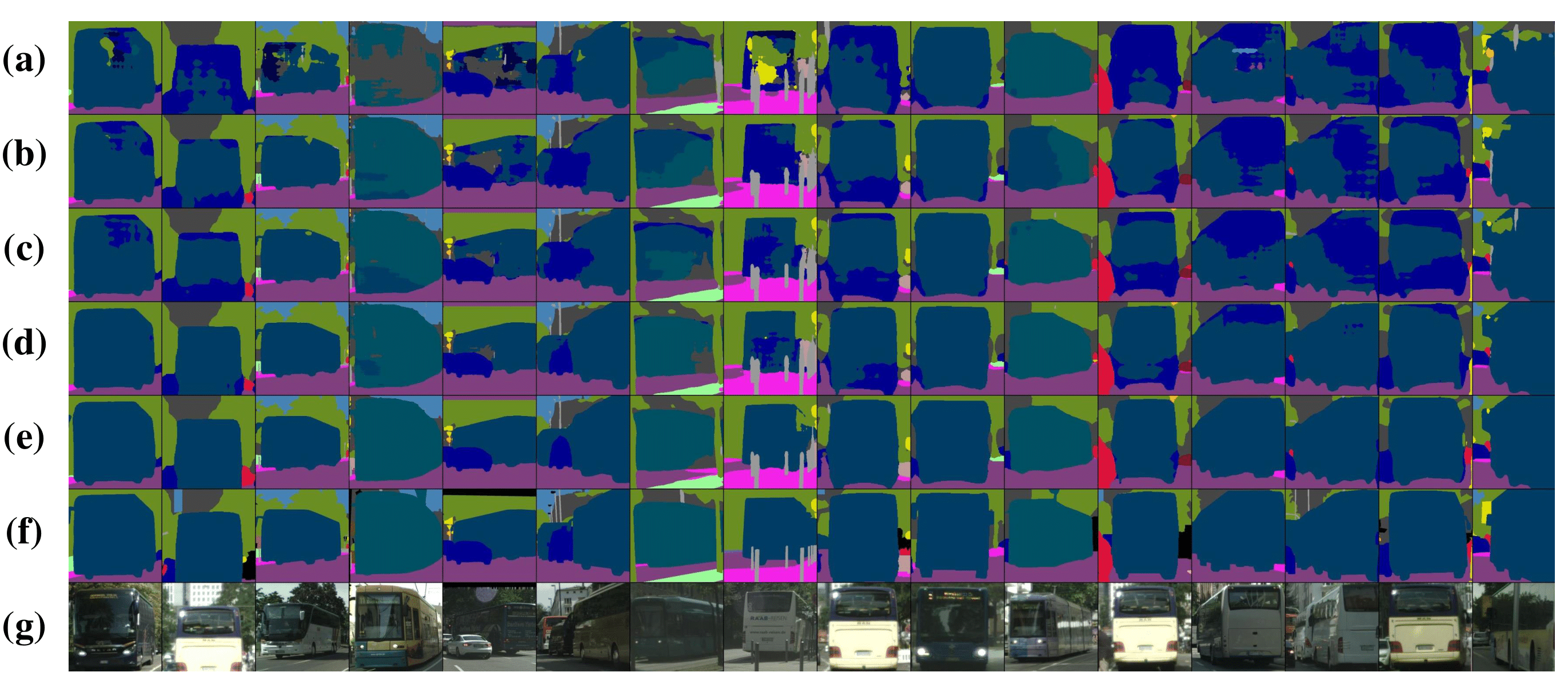
(a) Bus

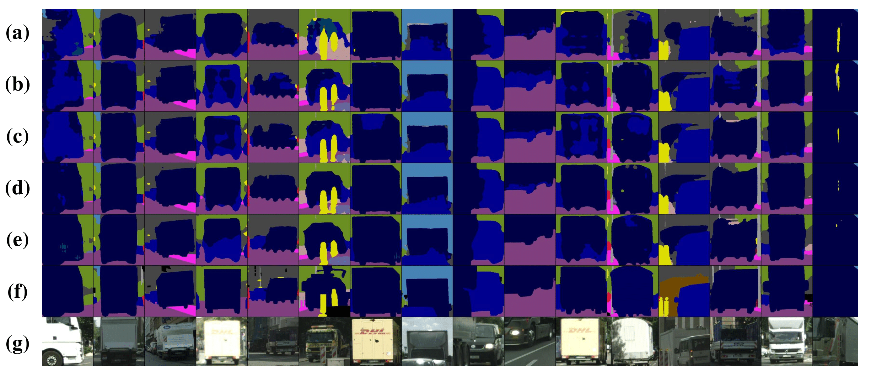
(b) Truck

Figure 6: Segmentation results for structured objects with ResNet$18$ ($1.0$) trained with different discriminators. (a) W/o holistic distillation, (b) W/ D_shallow, (c) W/ D_no_attention, (d) Our method, (e) Teacher net, (f) Ground truth, (g) Image. One can see a strong discriminator can help the student learn structure objects better. With the attention layers, labels of the objects are more consistent.

Feature and local pair-wise distillation. We compare a few variants of the pair-wise distillation:

• Feature distillation by MIMIC [19, 11]: We follow [11] to align the features of each pixel between $\mathsf{T}$ and $\mathsf{S}$ through a $1\times 1$ convolution layer to match the dimension of the feature

• Feature distillation by attention transfer [44]: We aggregate the response maps into an attention map (single channel), and then transfer the attention map from the teacher to the student.

• Local pair-wise distillation [12]: This method can be seen as a special case of our pair-wise distillation, which only cover a small sub-graph ($8$-neighborhood pixels for each node).

TABLE VI: Comparison of feature transfer MIMIC [19, 11], attention transfer [44], and local pair-wise distillation [12] against our pair-wise distillation. The segmentation is evaluated by mIoU (%). PI: pixel-wise distillation. MIMIC: using a $1\times 1$ convolution layer for feature distillation. AT: attention transfer for feature distillation. LOCAL: local similarity distillation method. PA: our pair-wise distillation. ImN: initializing the network from the weights pretrained on ImageNet dataset.

Method	ResNet$18$ ($0.5$)	ResNet$18$ ($1.0$) + ImN
w/o distillation	$55.37$	$69.10$
+ PI	$57.07$	$70.51$
+ PI + MIMIC	$58.44$	$71.03$
+ PI + AT	$57.93$	$70.70$
+ PI + LOCAL	$58.62$	$70.86$
+ PI + PA	$\bf{61}.\bf{52}$	$\bf{71}.\bf{78}$

We replace our pair-wise distillation by the above three distillation schemes to verify the effectiveness of our pair-wise distillation. From Table VI, we can see that our pair-wise distillation method outperforms all the other distillation methods. The superiority over feature distillation schemes (MIMIC [11] and attention transfer [44], which transfers the knowledge for each pixel separately) may be due the fact that we transfer the structured knowledge other than aligning the feature for each individual pixel. The superiority over the local pair-wise distillation shows the effectiveness of our fully connected pare-wise distillation, which is able to transfer the overall structure information other than a local boundary information [12].

TABLE VII: The segmentation results on the testing, validation (Val.) set of Cityscapes.

Method	#Params (M)	FLOPs (B)	Test §	Val.
Current state-of-the-art results
ENet [6] †	$0.3580$	$3.612$	$58.3$	n/a
ERFNet [23] ‡	$2.067$	$25.60$	$68.0$	n/a
FCN [1] ‡	$134.5$	$333.9$	$65.3$	n/a
RefineNet [4] ‡	$118.1$	$525.7$	$73.6$	n/a
OCNet [17]‡	$62.58$	$548.5$	$80.1$	n/a
PSPNet [3] ‡	$70.43$	$574.9$	$78.4$	n/a
Results w/ and w/o distillation schemes
MD [12] ‡	$14.3$5	$64.48$	n/a	$67.3$
MD (Enhanced) [12] ‡	$14.35$	$64.48$	n/a	$71.9$
ESPNet-C [15] †	$0.3492$	$3.468$	$51.1$	$53.3$
ESPNet-C (ours) †	$0.3492$	$3.468$	$57.6$	$59.9$
ESPNet [15] †	$0.3635$	$4.422$	$60.3$	$61.4$
ESPNet (ours) †	$0.3635$	$4.422$	$62.0$	$63.8$
ResNet$18$ ($0.5$) †	$3.835$	$33.35$	$54.1$	$55.4$
ResNet$18$ ($0.5$) (ours) †	$3.835$	$33.35$	$61.4$	$62.7$
ResNet18 (1.0) ‡	$15.24$	$128.2$	$67.6$	$69.1$
ResNet18 (1.0) (ours) ‡	$15.24$	$128.2$	$73.1$	$75.3$
MobileNetV$2$Plus [16] ‡	$8.301$	$86.14$	$68.9$	$70.1$
MobileNetV$2$Plus (ours) ‡	$8.301$	$86.14$	$74.0$	$74.5$

• Train from scratch

• Initialized from the weights pretrained on ImageNet

• We select a best model along training on validation set to submit to the leader board. All our models are test on single scale. Some teacher networks are test on multiple scales, such as OCNet and PSPNet.

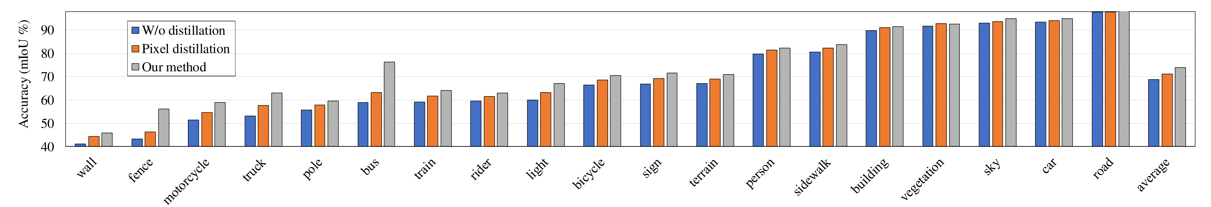
Figure 7: Illustrations of the effectiveness of structured distillation schemes in terms of class IoU scores using the network MobileNetV2Plus [16] on the Cityscapes test set. Both pixel-level and structured distillation are helpful for improving the performance especially for the hard classes with low IoU scores. The improvement from structured distillation is more significant for structured objects, such as bus and truck.

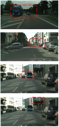
(a) Image

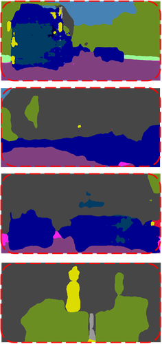
(b) W/o distillation

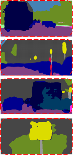
(c) Pixel-wise distillation

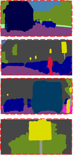
(d) Our method

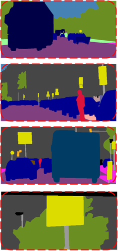
(e) Ground truth

Figure 8: Qualitative results on the Cityscapes testing set produced from MobileNetV2Plus: (a) initial images, (b) w/o distillation, (c) only w/ pixel-wise distillation, (d) Our distillation schemes: both pixel-wise and structured distillation schemes. The segmentation map in the red box about four structured objects: trunk, person, bus and traffic sign are zoomed in. One can see that the structured distillation method (ours) produces more consistent labels.

3.1.5 Segmentation Results

Cityscapes. We apply our structure distillation method to several compact networks: MobileNetV2Plus [16] which is based on a MobileNetV2 model, ESPNet-C [15] and ESPNet [15] which are carefully designed for mobile applications. Table VII presents the segmentation accuracy, the model complexity and the model size. FLOPs is calculated on the resolution of $512\times 1024$ pixels to evaluate the complexity. #Params is the number of network parameters. We can see that our distillation approach can improve the results over $5$ compact networks: ESPNet-C and ESPNet [15], ResNet$18$ ($0.5$), ResNet$18$ ($1.0$), and MobileNetV2Plus [16]. For the networks without pre-training, such as ResNet$18$ ($0.5$) and ESPNet-C, the improvements are very significant with $7.3\%$ and $6.6\%$, respectively. Compared with MD (Enhanced) [12] that uses the pixel-wise and local pair-wise distillation schemes over MobileNet, our approach with the similar network MobileNetV2Plus achieves higher segmentation quality ($74.5$ vs.  $71.9$ on the validation set) with a little higher computation complexity and much smaller model size.

Figure 7 shows the IoU scores for each class over MobileNetV2Plus. Both the pixel-wise and structured distillation schemes improve the performance, especially for the categories with low IoU scores. In particular, the structured distillation (pair-wise and holistic) has significant improvement for structured objects, e.g., $17.23\%$ improvement for Bus and $10.03\%$ for Truck. The qualitative segmentation results in Figure 8 visually demonstrate the effectiveness of our structured distillation for structured objects, such as trucks, buses, persons, and traffic signs.

CamVid. Table VIII shows the performance of the student networks w/o and w/ our distillation schemes and state-of-the-art results. We train and evaluate the student networks w/ and w/o distillation at the resolution $480\times 360$ following the setting of ENet. Again we can see that the distillation scheme improves the performance. Figure 9 shows some samples on the CamVid test set w/o and w/ the distillation produced from ESPNet.

TABLE VIII: The segmentation performance on the test set of CamVid. ‘ImN’: ImageNet dataset; ‘unl’: unlabeled street scene dataset sampled from Cityscapes.

Method	Extra data	mIoU (%)	#Params (M)
ENet[6]	no	$51.3$	$0.3580$
FC-DenseNet$56$[64]	no	$58.9$	$1.550$
SegNet[13]	ImN	$55.6$	$29.46$
DeepLab-LFOV[65]	ImN	$61.6$	$37.32$
FCN-$8$s[1]	ImN	$57.0$	$134.5$
ESPNet-C[15]	no	$56.7$
ESPNet-C (ours)	no	$60.3$	$0.3492$
ESPNet-C (ours)	unl	$64.1$
ESPNet[15]	no	$57.8$
ESPNet (ours)	no	$61.4$	$0.3635$
ESPNet (ours)	unl	$65.1$
ResNet$18$	ImN	$70.3$
ResNet$18$ (ours)	ImN	$71.0$	$15.24$
ResNet$18$ (ours)	ImN+unl	$72.3$

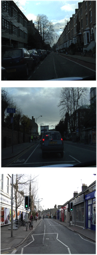
(a) Image

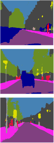
(b) W/o dis.

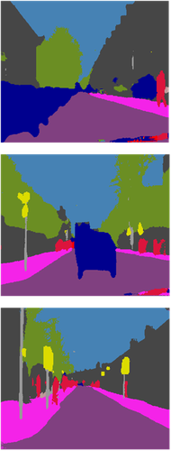
(c) Our method

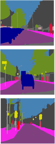
(d) Ground truth

Figure 9: Qualitative results on the CamVid test set produced from ESPNet. W/o dis. represents for the baseline student network trained without distillation.

We also conduct an experiment by using an extra unlabeled dataset, which contains $2000$ unlabeled street scene images collected from the Cityscapes dataset, to show that the distillation schemes can transfer the knowledge of the unlabeled images. The experiments are done with ESPNet and ESPNet-C. The loss function is almost the same except that there is no cross-entropy loss over the unlabeled dataset. The results are shown in Figure 10. We can see that our distillation method with the extra unlabeled data can significantly improve mIoU of ESPNet-C and ESPNet for $13.5\%$ and $12.6\%$.

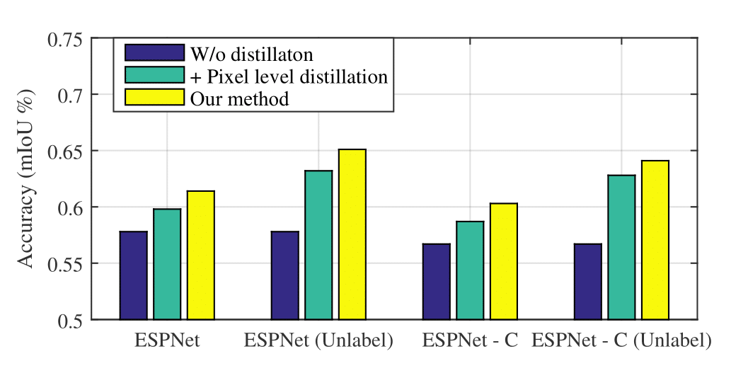
Figure 10: The effect of structured distillation on CamVid. This figure shows that distillation can improve the results in two cases: trained over only the labeled data and over both the labeled and extra unlabeled data.

ADE$20$K. The ADE$20$K dataset is a very challenging dataset and contains $150$ categories of objects. Note that the number of pixels belonging to difference categories in this dataset is very imbalanced.

We report the results for ResNet$18$ and the MobileNetV$2$ which are trained with the initial weights pretrained on the ImageNet dataset, and ESPNet which is trained from scratch in Table IX. We follow the same training scheme in [66]. All results are tested on single scale. For ESPNet, with our distillation, we can see that the mIoU score is improved by $3.78\%$, and it achieves a higher accuracy with fewer parameters compared to SegNet. For ResNet$18$ and MobileNetV$2$, after the distillation, we achieve $2.73\%$ improvement over the one without distillation reported in [66].

TABLE IX: The mIoU and pixel accuracy on validation set of ADE$20$K.

Method	mIoU(%)	Pixel Acc. (%)	#Params (M)
SegNet [13]	$21.64$	$71.00$	$29.46$
DilatedNet$50$ [66]	$34.28$	$76.35$	$62.74$
PSPNet (teacher) [3]	$42.19$	$80.59$	$70.43$
FCN [1]	$29.39$	$71.32$	$134.5$
ESPNet [15]	$20.13$	$70.54$	$0.3635$
ESPNet (ours)	$24.29$	$72.86$	$0.3635$
MobileNetV$2$ [66]	$34.84$	$75.75$	$2.17$
MobileNetV$2$ (ours)	$38.58$	$79.78$	$2.17$
ResNet$18$ [66]	$33.82$	$76.05$	$12.25$
ResNet$18$ (ours)	$36.60$	$77.97$	$12.25$

(a) Image

(b) w/o dis.

(c) Our method

Figure 11: Qualitative results on the ADE$20$K produced from MobileNetV$2$. W/o dis.  represents for the baseline student network trained without distillation.

3.2 Depth Estimation

3.2.1 Implementation Details

Network structures. We use the same model described in [37] with the ResNext$101$ backbone as our teacher model, and replace the backbone with MobileNetV$2$ as the compact model.

Training details. We train the student net using the crop size $385\times 385$ by mini-batch stochastic gradient descent (SGD) with batchsize of $12$. The initialized learning rate is $0.001$ and is multiplied by $(1-\frac{iter}{max-iter})^{0.9}$. For both w/ and w/o distillation methods, the training epoch is $200$.

3.2.2 Dataset

NYUD-V2. The NYUD-V2 dataset contains $1449$ annotated indoor images, in which $795$ images are for training and others are for testing. The image size is $640\times 480$. Some methods have sampled more images from the video sequence of NYUD-V2 to form a Large-NYUD-V2 to further improve the performance. Following [37], we conduct ablation studies on the small dataset and also apply the distillation method on current state-of-the-art real-time depth models trained with Large-NYUD-V2 to verify the effectiveness of the structured knowledge distillation.

3.2.3 Evaluation Metrics

We follow previous methods [37] to evaluate the performance of monocular depth estimation quantitatively based on following metrics: mean absolute relative error (rel), mean $\log_{10}$ error ($\log_{10}$), root mean squared error (rms) , and the accuracy under threshold ($\delta_{i}<1.25^{i},i=1,2,3$).

3.2.4 Results

Ablation studies. We compare the pixel-wise distillation and the structured knowledge distillation in this section. In the dense classification problem, e.g., semantic segmentation, the output logits of the teacher is a soft distribution of all the classes, which contain the relations among different classes. Therefore, directly transfer the logits from teacher models from the compact ones at the pixel level can help improve the performance. Different from semantic segmentation, as the depth map are real values, the output of the teacher is often not as accurate as ground truth labels. In the experiments, we find that adding pixel-level distillation hardly improves the accuracy in the depth estimation task. Thus, we only use the structured knowledge distillation in depth estimation task.

To verify that the distillation method can further improve the accuracy with unlabeled data, we use $30K$ image sampled from the video sequence of NYUD-V2 without the depth map. The results are shown in Table X. We can see that the structured knowledge distillation performs better than pixel-wise distillation, and adding extra unlabelled data can further improve the accuracy.

TABLE X: Depth estimation. Relative error on the NYUD-V2 test dataset. ‘Unl’ means Unleblled data sampled from the large video sequence. The pixel-level distillation alone can not improve the accuracy. Therefore we only use structured-knowledge distillation in the depth estimation task.

Method	Baseline	PI	+PA	+PA +HO	+PA +HO +Unl
rel	$0.181$	$0.183$	$0.175$	$0.173$	$\bf{0.160}$

Comparison with state-of-the-art. We apply the distillation method to a few state-of-the-art lightweight models for depth estimation. Following [37], we train the student net on Large-NYUD-V2 with the same constraints in [37] as our baseline, and achieve $13.5$ in the metric ‘rel’. Following the same training setups, with the structured knowledge distillation terms, we further improve the strong baseline, and achieve a relative error (rel) of $13.0$. In Table XI, we list the model parameters and accuracy of a few state-of-the-art large models along with some real-time models, indicating that the structured knowledge distillation works on a strong baseline.

TABLE XI: Depth estimation results and model parameters on NYUD-V2 test dataset. With the structured knowledge distillation, the performance is improved over all evaluation metrics.

Method	backbone	#Params (M)	rel	log10	rms	$\boldsymbol{\delta_{1}}$	$\boldsymbol{\delta_{2}}$	$\boldsymbol{\delta_{3}}$
			Lower is better			Higher is better
Laina et al. [67]	ResNet$50$	$60.62$	$0.127$	$0.055$	$0.573$	$0.811$	$0.953$	$0.988$
DORN [35]	ResNet$101$	$105.17$	$0.115$	$0.051$	$0.509$	$0.828$	$0.965$	$0.992$
AOB [68]	SENET-$154$	$149.820.181$	$0.115$	$0.050$	$0.530$	$0.866$	$0.975$	$0.993$
VNL (teacher) [37]	ResNext$101$	$86.24$	$\bf{0.108}$	$\bf{0.048}$	$\bf{0.416}$	$\bf{0.875}$	$\bf{0.976}$	$\bf{0.994}$
CReaM [38]	-	$\bf{1.5}$	$0.190$	-	$0.687$	$0.704$	$0.917$	$0.977$
RF-LW [69]	MobileNetV$2$	$3.0$	$0.149$	-	$0.565$	$0.790$	$0.955$	$0.990$
VNL (student)	MobileNetV$2$	$2.7$	$0.135$	$0.060$	$0.576$	$0.813$	$0.958$	$0.991$
VNL (student) w/ distillation	MobileNetV$2$	$2.7$	$\bf{0.130}$	$\bf{0.055}$	$\bf{0.544}$	$\bf{0.838}$	$\bf{0.971}$	$\bf{0.994}$

3.3 Object Detection

3.3.1 Implementation Details

Network structures. We experiment with the recent one-stage architecture FCOS [5], using the backbone ResNeXt-$32$x$8$d-$101$-FPN as the teacher network. The channel in the detector towers is set to $256$. It is a simple anchor-free model, but can achieve comparable performance with state-of-the-art two-stage detection methods.

We choose two different models based on the MobileNetV$2$ backbone: c$128$-MNV$2$ and c$256$-MNV$2$ released by FCOS [5] as our student nets, where $c$ represents the channel in the detector towers. We apply the distillation loss on all the output levels of the feature pyramid network.

Training setup. We follow the training schedule in FCOS [5]. For ablation studies, all the teacher, the student w/ and w/o distillation are trained with stochastic gradient descent (SGD) for $90$K iterations with the initial learning rate being $0.01$ and a mini batch of $16$ images. The learning rate is reduced by a factor of $10$ at iteration $60$K and $80$K, respectively. Weight decay and momentum are set to be $0.0001$ and $0.9$, respectively. To compare with other state-of-the-art real-time detectors, we double the training iterations and the batch size, and the distillation method can further improve the results on the strong baselines.

3.3.2 Dataset

COCO. Microsoft Common Objects in Context (COCO) [70] is a large-scale detection benchmark in object detection. There are $115K$ images for training and $5K$ images for validation. We evaluate the ablation results on the validation set, and we also submit the final results to the test-dev of COCO.

3.3.3 Evaluation Metrics

Average precision (AP) computes the average precision value for recall value over $0$ to $1$. The mAP is the averaged AP over multiple Intersection over Union (IoU) values, from $0.5$ to $0.95$ with a step of $0.05$. We also report AP$50$ and AP$75$ represents for the AP with a single IoU of $0.5$ and $0.75$, respectively. APs, APm and APl are AP across different scales for small, medium and large objects.

TABLE XII: Object detection. PA vs.  MIMIC on the COCO-minival split with MobileNetV$2$-c$256$ as the student net. Both distillation method can improve the accuracy of the detector, and the structured knowledge distillation performs better than the pixel-wise MIMIC. By applying all the distillation terms, the results can be further improved.

Method	mAP	AP50	AP75	APs	APm	APl
Teacher	$42.5$	$61.7$	$45.9$	$26.0$	$46.2$	$54.3$
student	$31.0$	$48.5$	$32.7$	$17.1$	$34.2$	$39.7$
+MIMIC [11]	$31.4$	$48.1$	$33.4$	$16.5$	$34.3$	$41.0$
+PA	$31.9$	$49.2$	$33.7$	$17.7$	$34.7$	$\bf{41.3}$
Ours	$\bf{32.1}$	$\bf{49.5}$	$\bf{34.2}$	$\bf{18.5}$	$\bf{35.3}$	$41.2$

3.3.4 Results

Comparison with different distillation methods. To demonstrate the effectiveness of the structured knowledge distillation, we compare the pair-wise distillation method with the previous MIMIC [11] method, which aligns the feature map on pixel-level. We use the c$256$-MNV$2$ as the student net and the results are shown in Table XII. By adding the pixel-wise MIMIC distillation method, the detector can be improved by $0.4\%$ in mAP. Our structured knowledge distillation method can improve by $0.9\%$ in mAP. Under all evaluation metrics, the structured knowledge distillation method performs better than MIMIC. By combing the structured knowledge distillation with the pixel-wise distillation, the results can be further improved to $32.1\%$ mAP. Comparing to the baseline method without distillation, the improvement of AP$75$, APs and APl are more sound, indicating the effectiveness of the distillation method.

We show some detection results in Figure 12. One can see that the detector trained with our distillation method can detect more small objects such as ‘person’ and ‘bird’.

TABLE XIII: Detection accuracy with and without distillation on COCO-minival.

Method	mAP	AP$50$	AP$75$	APs	APm	APl
Teacher	$42.5$	$61.7$	$45.9$	$26.0$	$46.2$	$54.3$
C$128$-MV$2$	$30.9$	$48.5$	$32.7$	$17.1$	$34.2$	$39.7$
w/ distillation	$31.8$	$49.2$	$33.8$	$17.8$	$35.0$	$40.4$
C$256$-MV$2$	$33.1$	$51.1$	$35.0$	$18.5$	$36.1$	$43.4$
w/ distillation	$33.9$	$51.8$	$35.7$	$19.7$	$37.3$	$43.4$

Results of different student nets. We follow the same training steps ($90$K) and batch size ($32$) as in FCOS [5] and apply the distillation method on two different structures: C$256$-MV$2$ and C$128$-MV$2$. The results of w/ and w/o distillation are shown in Table XIII. By applying the structured knowledge distillation combine with pixel-wise distillation, the mAP of C$128$-MV$2$ and and C$256$-MV$2$ are improved by $0.9$ and $0.8$, respectively.

TABLE XIV: Detection results and inference time on the COCO test-dev. The inference time was reported in the original papers [5, 41]. Our distillation method can improve the accuracy of a strong baseline with no extra inference time.

	backbone	AP	AP50	AP75	APS	APM	APL	time (ms/img)
RetinaNet [41]	ResNet-$101$-FPN	$39.1$	$59.1$	$42.3$	$21.8$	$42.7$	$50.2$	$198$
RetinaNet [41]	ResNeXt-$101$-FPN	$40.8$	$61.1$	$44.1$	$24.1$	$44.2$	$51.2$	-
FCOS [5] (teacher)	ResNeXt-$101$-FPN	$\bf{42.7}$	$\bf{62.2}$	$\bf{46.1}$	$\bf{26.0}$	$\bf{45.6}$	$\bf{52.6}$	$\bf{130}$
YOLOv$2$ [71]	DarkNet-$19$	$21.6$	$44.0$	$19.2$	$5.0$	$22.4$	$35.5$	$\bf{25}$
SSD$513$ [9]	ResNet-$101$-SSD	$31.2$	$50.4$	$33.3$	$10.2$	$34.5$	$49.8$	$125$
DSSD$513$ [72]	ResNet-$101$-DSSD	$33.2$	$53.3$	$35.2$	$13.0$	$35.4$	$51.1$	$156$
YOLOv$3$ [73]	Darknet-$53$	$33.0$	$\bf{57.9}$	$34.4$	$18.3$	$35.4$	$41.9$	$51$
FCOS (student) [5]	MobileNetV$2$-FPN	$31.4$	$49.2$	$33.3$	$17.1$	$33.5$	$38.8$	$45$
FCOS (student) w/ distillation	MobileNetV$2$-FPN	$\bf{34.1}$	$52.2$	$\bf{36.4}$	$\bf{19.0}$	$\bf{36.2}$	$\bf{42.0}$	$45$

(a) Detection results w/o distillation

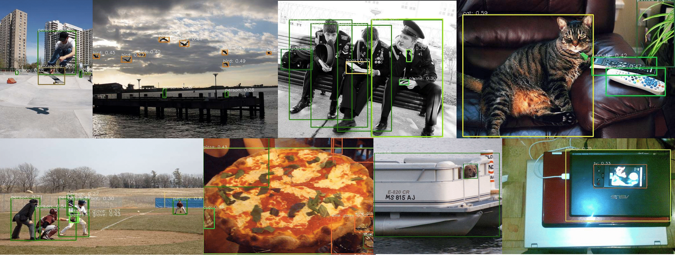
(b) Detection results w/ distillation

Figure 12: Detection results on the COCO dataset. With the structured knowledge distillation, the detector’s accuracy is improved, particularly for detecting occluded, highly overlapped and extremely small objects.

Results on the test-dev. The original mAP on the validation set of C$128$-MV$2$ reported by FCOS is $30.9\%$ with $90$K iterations. We double the training iterations and train with the distillation method. The final mAP on minival is $33.9\%$. The test results are in Table XIV, and we also list the AP and inference time for some state-of-the-art one-stage detectors to show the position of the baseline and our detectors trained with the structured knowledge distillation method. To make a fair comparison, we also double the training iterations without any distillation methods, and obtain mAP of $32.7\%$ on minival.

4 Conclusion

We have studied knowledge distillation for training compact dense prediction networks with the help of cumbersome/teacher networks. By considering the structure information in dense prediction, we have presented two structural distillation schemes: pair-wise distillation and holistic distillation. We demonstrate the effectiveness of our proposed distillation schemes on several recent compact networks on three dense prediction tasks: semantic segmentation, depth estimation and object detection. Our structured knowledge distillation methods are complimentary to traditional pixel-wise distillation methods.

Yifan Liu is a Ph.D candidate in Computer Science at The University of Adelaide, supervised by Professor Chunhua Shen. She obtained her B.S. and M.Sc. in Artificial Intelligence from Beihang University. Her research interests include image processing, dense prediction and real-time applications in deep learning.

Changyong Shu received the Ph.D. degree from Beihang University, Beijing, China, in 2017. He has been with the Nanjing Institute of Advanced Artificial Intelligence since 2018. His current research interest focuses on knowledge distillation.

Jingdong Wang is a Senior Principal Research Manager with the Visual Computing Group, Microsoft Research, Beijing, China. He received the B.Eng. and M.Eng. degrees from the Department of Automation, Tsinghua University, Beijing, China, in 2001 and 2004, respectively, and the PhD degree from the Department of Computer Science and Engineering, the Hong Kong University of Science and Technology, Hong Kong, in 2007. His areas of interest include deep learning, large-scale indexing, human understanding, and person re-identification. He is an Associate Editor of IEEE TPAMI, IEEE TMM and IEEE TCSVT, and is an area chair (or SPC) of some prestigious conferences, such as CVPR, ICCV, ECCV, ACM MM, IJCAI, and AAAI. He is a Fellow of IAPR and an ACM Distinguished Member.

Chunhua Shen is a Professor at School of Computer Science, The University of Adelaide, Australia.

References

- [1] E. Shelhamer, J. Long, and T. Darrell, “Fully convolutional networks for semantic segmentation.” IEEE Trans. Pattern Anal. Mach. Intell., vol. 39, no. 4, p. 640, 2017.
- [2] L.-C. Chen, G. Papandreou, I. Kokkinos, K. Murphy, and A. L. Yuille, “Deeplab: Semantic image segmentation with deep convolutional nets, atrous convolution, and fully connected crfs,” IEEE Trans. Pattern Anal. Mach. Intell., vol. 40, no. 4, pp. 834–848, 2018.
- [3] H. Zhao, J. Shi, X. Qi, X. Wang, and J. Jia, “Pyramid scene parsing network,” in Proc. IEEE Conf. Comp. Vis. Patt. Recogn., 2017, pp. 2881–2890.
- [4] G. Lin, F. Liu, A. Milan, C. Shen, and I. Reid, “Refinenet: Multi-path refinement networks for dense prediction,” IEEE Trans. Pattern Anal. Mach. Intell., 2019.
- [5] Z. Tian, C. Shen, H. Chen, and T. He, “FCOS: Fully convolutional one-stage object detection,” Proc. IEEE Int. Conf. Comp. Vis., 2019.
- [6] A. Paszke, A. Chaurasia, S. Kim, and E. Culurciello, “Enet: A deep neural network architecture for real-time semantic segmentation,” arXiv: Comp. Res. Repository, vol. abs/1606.02147, 2016.
- [7] H. Zhao, X. Qi, X. Shen, J. Shi, and J. Jia, “Icnet for real-time semantic segmentation on high-resolution images,” Proc. Eur. Conf. Comp. Vis., 2018.
- [8] J. Redmon, S. Divvala, R. Girshick, and A. Farhadi, “You only look once: Unified, real-time object detection,” in Proc. IEEE Conf. Comp. Vis. Patt. Recogn., 2016, pp. 779–788.
- [9] W. Liu, D. Anguelov, D. Erhan, C. Szegedy, S. Reed, C.-Y. Fu, and A. C. Berg, “Ssd: Single shot multibox detector,” in Proc. Eur. Conf. Comp. Vis. Springer, 2016, pp. 21–37.
- [10] D. Wofk, F. Ma, T.-J. Yang, S. Karaman, and V. Sze, “Fastdepth: Fast monocular depth estimation on embedded systems,” Int. Conf. on Robotics and Automation, 2019.
- [11] Q. Li, S. Jin, and J. Yan, “Mimicking very efficient network for object detection,” Proc. IEEE Conf. Comp. Vis. Patt. Recogn., pp. 7341–7349, 2017.
- [12] J. Xie, B. Shuai, J.-F. Hu, J. Lin, and W.-S. Zheng, “Improving fast segmentation with teacher-student learning,” Proc. British Machine Vis. Conf., 2018.
- [13] V. Badrinarayanan, A. Kendall, and R. Cipolla, “Segnet: A deep convolutional encoder-decoder architecture for image segmentation,” IEEE Trans. Pattern Anal. Mach. Intell., no. 12, pp. 2481–2495, 2017.
- [14] E. Romera, J. M. Alvarez, L. M. Bergasa, and R. Arroyo, “Efficient convnet for real-time semantic segmentation,” in IEEE Intelligent Vehicles Symp., 2017, pp. 1789–1794.
- [15] S. Mehta, M. Rastegari, A. Caspi, L. Shapiro, and H. Hajishirzi, “Espnet: Efficient spatial pyramid of dilated convolutions for semantic segmentation,” Proc. Eur. Conf. Comp. Vis., 2018.
- [16] H. Liu, “Lightnet: Light-weight networks for semantic image segmentation,” https://github.com/ansleliu/LightNet, 2018.
- [17] Y. Yuan and J. Wang, “Ocnet: Object context network for scene parsing,” in arXiv: Comp. Res. Repository, vol. abs/1809.00916, 2018.
- [18] G. E. Hinton, O. Vinyals, and J. Dean, “Distilling the knowledge in a neural network,” arXiv: Comp. Res. Repository, vol. abs/1503.02531, 2015.
- [19] A. Romero, N. Ballas, S. E. Kahou, A. Chassang, C. Gatta, and Y. Bengio, “Fitnets: Hints for thin deep nets,” arXiv: Comp. Res. Repository, vol. abs/1412.6550, 2014.
- [20] S. Z. Li, Markov random field modeling in image analysis. Springer Science & Business Media, 2009.
- [21] K. He, X. Zhang, S. Ren, and J. Sun, “Deep residual learning for image recognition,” Proc. IEEE Conf. Comp. Vis. Patt. Recogn., pp. 770–778, 2016.
- [22] G. Huang, Z. Liu, L. van der Maaten, and K. Q. Weinberger, “Densely connected convolutional networks,” Proc. IEEE Conf. Comp. Vis. Patt. Recogn., pp. 2261–2269, 2017.
- [23] F. Yu and V. Koltun, “Multi-scale context aggregation by dilated convolutions,” Proc. Int. Conf. Learn. Representations, 2016.
- [24] G. Lin, C. Shen, A. van den Hengel, and I. Reid, “Efficient piecewise training of deep structured models for semantic segmentation,” in Proc. IEEE Conf. Comp. Vis. Patt. Recogn., 2016, pp. 3194–3203.
- [25] C. Szegedy, V. Vanhoucke, S. Ioffe, J. Shlens, and Z. Wojna, “Rethinking the inception architecture for computer vision,” Proc. IEEE Conf. Comp. Vis. Patt. Recogn., pp. 2818–2826, 2016.
- [26] M. Treml, J. Arjona-Medina, T. Unterthiner, R. Durgesh, F. Friedmann, P. Schuberth, A. Mayr, M. Heusel, M. Hofmarcher, M. Widrich et al., “Speeding up semantic segmentation for autonomous driving,” in Proc. Workshop of Advances in Neural Inf. Process. Syst., 2016.
- [27] F. N. Iandola, M. W. Moskewicz, K. Ashraf, S. Han, W. J. Dally, and K. Keutzer, “Squeezenet: Alexnet-level accuracy with 50x fewer parameters and <1mb model size,” arXiv: Comp. Res. Repository, vol. abs/1602.07360, 2016.
- [28] A. G. Howard, M. Zhu, B. Chen, D. Kalenichenko, W. Wang, T. Weyand, M. Andreetto, and H. Adam, “Mobilenets: Efficient convolutional neural networks for mobile vision applications,” arXiv: Comp. Res. Repository, vol. abs/1704.04861, 2017.
- [29] X. Zhang, X. Zhou, M. Lin, and J. Sun, “Shufflenet: An extremely efficient convolutional neural network for mobile devices,” Proc. IEEE Conf. Comp. Vis. Patt. Recogn., 2018.
- [30] A. Saxena, M. Sun, and A. Y. Ng, “Learning 3-d scene structure from a single still image,” in Proc. IEEE Int. Conf. Comp. Vis. IEEE, 2007, pp. 1–8.
- [31] D. Eigen, C. Puhrsch, and R. Fergus, “Depth map prediction from a single image using a multi-scale deep network,” in Proc. Advances in Neural Inf. Process. Syst., 2014.
- [32] F. Liu, C. Shen, and G. Lin, “Deep convolutional neural fields for depth estimation from a single image,” in Proc. IEEE Conf. Comp. Vis. Patt. Recogn., 2015.
- [33] F. Liu, C. Shen, G. Lin, and I. Reid, “Learning depth from single monocular images using deep convolutional neural fields,” IEEE Trans. Pattern Anal. Mach. Intell., 2016.
- [34] R. Li, K. Xian, C. Shen, Z. Cao, H. Lu, and L. Hang, “Deep attention-based classification network for robust depth prediction,” in Proc. Asian Conf. Comp. Vis., 2018.
- [35] H. Fu, M. Gong, C. Wang, K. Batmanghelich, and D. Tao, “Deep ordinal regression network for monocular depth estimation,” in Proc. IEEE Conf. Comp. Vis. Patt. Recogn., 2018, pp. 2002–2011.
- [36] X. Fei, A. Wang, and S. Soatto, “Geo-supervised visual depth prediction,” in arXiv: Comp. Res. Repository, vol. abs/1807.11130, 2018.
- [37] Y. Wei, Y. Liu, C. Shen, and Y. Yan, “Enforcing geometric constraints of virtual normal for depth prediction,” Proc. IEEE Int. Conf. Comp. Vis., 2019.
- [38] A. Spek, T. Dharmasiri, and T. Drummond, “Cream: Condensed real-time models for depth prediction using convolutional neural networks,” in Int. Conf. on Intell. Robots and Sys. IEEE, 2018, pp. 540–547.
- [39] R. Girshick, “Fast r-cnn,” in Proc. IEEE Int. Conf. Comp. Vis., 2015, pp. 1440–1448.
- [40] S. Ren, K. He, R. Girshick, and J. Sun, “Faster r-cnn: Towards real-time object detection with region proposal networks,” in Proc. Advances in Neural Inf. Process. Syst., 2015, pp. 91–99.
- [41] T.-Y. Lin, P. Goyal, R. Girshick, K. He, and P. Dollár, “Focal loss for dense object detection,” in Proc. IEEE Int. Conf. Comp. Vis., 2017, pp. 2980–2988.
- [42] J. Ba and R. Caruana, “Do deep nets really need to be deep?” in Proc. Advances in Neural Inf. Process. Syst., 2014, pp. 2654–2662.
- [43] G. Urban, K. J. Geras, S. E. Kahou, O. Aslan, S. Wang, R. Caruana, A. Mohamed, M. Philipose, and M. Richardson, “Do deep convolutional nets really need to be deep (or even convolutional)?” in Proc. Int. Conf. Learn. Representations, 2016.
- [44] S. Zagoruyko and N. Komodakis, “Paying more attention to attention: Improving the performance of convolutional neural networks via attention transfer,” Proc. Int. Conf. Learn. Representations, 2017.
- [45] Y. Liu, K. Chen, C. Liu, Z. Qin, Z. Luo, and J. Wang, “Structured knowledge distillation for semantic segmentation,” in Proc. IEEE Conf. Comp. Vis. Patt. Recogn., 2019, pp. 2604–2613.
- [46] M. Sandler, A. Howard, M. Zhu, A. Zhmoginov, and L.-C. Chen, “Mobilenetv2: Inverted residuals and linear bottlenecks,” in Proc. IEEE Conf. Comp. Vis. Patt. Recogn., 2018.
- [47] H. Wang, Z. Qin, and T. Wan, “Text generation based on generative adversarial nets with latent variables,” in Proc. Pacific-Asia Conf. Knowledge discovery & data mining, 2018, pp. 92–103.
- [48] L. Yu, W. Zhang, J. Wang, and Y. Yu, “Seqgan: Sequence generative adversarial nets with policy gradient.” in Proc. AAAI Conf. Artificial Intell., 2017, pp. 2852–2858.
- [49] I. J. Goodfellow, J. Pougetabadie, M. Mirza, B. Xu, D. Wardefarley, S. Ozair, A. Courville, Y. Bengio, Z. Ghahramani, and M. Welling, “Generative adversarial nets,” Proc. Advances in Neural Inf. Process. Syst., vol. 3, pp. 2672–2680, 2014.
- [50] T. Karras, T. Aila, S. Laine, and J. Lehtinen, “Progressive growing of gans for improved quality, stability, and variation,” Proc. Int. Conf. Learn. Representations, 2018.
- [51] M. Mirza and S. Osindero, “Conditional generative adversarial nets,” arXiv: Comp. Res. Repository, vol. abs/1411.1784, 2014.
- [52] J. Johnson, A. Alahi, and L. Fei-Fei, “Perceptual losses for real-time style transfer and super-resolution,” Proc. Eur. Conf. Comp. Vis., pp. 694–711, 2016.
- [53] Y. Liu, Z. Qin, T. Wan, and Z. Luo, “Auto-painter: Cartoon image generation from sketch by using conditional wasserstein generative adversarial networks,” Neurocomputing, vol. 311, pp. 78–87, 2018.
- [54] Y. Chen, C. Shen, X.-S. Wei, L. Liu, and J. Yang, “Adversarial PoseNet: A structure-aware convolutional network for human pose estimation,” in Proc. IEEE Int. Conf. Comp. Vis., 2017, pp. 1212–1221.
- [55] P. Luc, C. Couprie, S. Chintala, and J. Verbeek, “Semantic segmentation using adversarial networks,” arXiv: Comp. Res. Repository, vol. abs/1611.08408, 2016.
- [56] K. Gwn Lore, K. Reddy, M. Giering, and E. A. Bernal, “Generative adversarial networks for depth map estimation from rgb video,” in Proc. IEEE Conf. Comp. Vis. Patt. Recogn., 2018, pp. 1177–1185.
- [57] I. Gulrajani, F. Ahmed, M. Arjovsky, V. Dumoulin, and A. C. Courville, “Improved training of wasserstein gans,” in Proc. Advances in Neural Inf. Process. Syst., 2017, pp. 5767–5777.
- [58] H. Zhang, I. Goodfellow, D. Metaxas, and A. Odena, “Self-attention generative adversarial networks,” in arXiv: Comp. Res. Repository, vol. abs/1805.08318, 2018.
- [59] Y. Cao, Z. Wu, and C. Shen, “Estimating depth from monocular images as classification using deep fully convolutional residual networks,” IEEE Trans. Circuits Syst. Video Technol., vol. 28, no. 11, pp. 3174–3182, 2017.
- [60] M. Cordts, M. Omran, S. Ramos, T. Rehfeld, M. Enzweiler, R. Benenson, U. Franke, S. Roth, and B. Schiele, “The cityscapes dataset for semantic urban scene understanding,” in Proc. IEEE Conf. Comp. Vis. Patt. Recogn., 2016.
- [61] G. J. Brostow, J. Shotton, J. Fauqueur, and R. Cipolla, “Segmentation and recognition using structure from motion point clouds,” in Proc. Eur. Conf. Comp. Vis. Springer, 2008, pp. 44–57.
- [62] B. Zhou, H. Zhao, X. Puig, S. Fidler, A. Barriuso, and A. Torralba, “Scene parsing through ade20k dataset,” in Proc. IEEE Conf. Comp. Vis. Patt. Recogn., 2017.
- [63] https://github.com/warmspringwinds/pytorch-segmentation-detection/blob/master/pytorch_segmentation_detection/utils/flops_benchmark.py, 2018.
- [64] S. J. M. Drozdzal, D. Vazquez, and A. R. Y. Bengio, “The one hundred layers tiramisu: Fully convolutional densenets for semantic segmentation,” Proc. Workshop of IEEE Conf. Comp. Vis. Patt. Recogn., 2017.
- [65] L.-C. Chen, G. Papandreou, I. Kokkinos, K. Murphy, and A. Yuille, “Semantic image segmentation with deep convolutional nets and fully connected crfs,” in Proc. Int. Conf. Learn. Representations, 2015.
- [66] T. Xiao, Y. Liu, B. Zhou, Y. Jiang, and J. Sun, “Unified perceptual parsing for scene understanding,” in Proc. Eur. Conf. Comp. Vis., 2018.
- [67] I. Laina, C. Rupprecht, V. Belagiannis, F. Tombari, and N. Navab, “Deeper depth prediction with fully convolutional residual networks,” in Proc. Int. Conf. 3D Vision (3DV). IEEE, 2016, pp. 239–248.
- [68] J. Hu, M. Ozay, Y. Zhang, and T. Okatani, “Revisiting single image depth estimation: Toward higher resolution maps with accurate object boundaries,” in Proc. Winter Conf. on Appl. of Comp0 Vis. IEEE, 2019, pp. 1043–1051.
- [69] V. Nekrasov, T. Dharmasiri, A. Spek, T. Drummond, C. Shen, and I. Reid, “Real-time joint semantic segmentation and depth estimation using asymmetric annotations,” in arXiv: Comp. Res. Repository, vol. abs/1809.04766, 2018.
- [70] T.-Y. Lin, M. Maire, S. Belongie, J. Hays, P. Perona, D. Ramanan, P. Dollár, and C. L. Zitnick, “Microsoft coco: Common objects in context,” in Proc. Eur. Conf. Comp. Vis. Springer, 2014, pp. 740–755.
- [71] J. Redmon and A. Farhadi, “Yolo9000: better, faster, stronger,” in Proc. IEEE Conf. Comp. Vis. Patt. Recogn., 2017, pp. 7263–7271.
- [72] C.-Y. Fu, W. Liu, A. Ranga, A. Tyagi, and A. C. Berg, “Dssd: Deconvolutional single shot detector,” in arXiv: Comp. Res. Repository, vol. abs/1701.06659, 2017.
- [73] J. Redmon and A. Farhadi, “Yolov3: An incremental improvement,” in arXiv: Comp. Res. Repository, vol. abs/1804.02767, 2018.