On calculating response functions via their Lorentz integral transforms

Abstract

The accuracy of reconstruction of a response function from its Lorentz integral transform is studied in an exactly solvable model. An inversion procedure is elaborated in detail and features of the procedure are studied. Unlike results in the literature pertaining to the same model, the response function is reconstructed from its Lorentz integral transform with rather high accuracy.

I introduction

We address the issue of computing the response functions

$$R(E)=\sum_{n}|(\Psi_{n},O\Psi_{0})|^{2}\delta(E-E_{n})+\sum\!\!\!\!\!\!\!\int df|(\Psi_{f},O\Psi_{0})|^{2}\delta(E-E_{f})$$ (1)

of quantum mechanical systems. Here $\Psi_{n}$ and $\Psi_{f}$ represent a complete set of bound plus continuum–spectrum states of the Hamiltonian of a problem, $\Psi_{0}$ is the initial state, and $O$ is a transition operator. The subscript $f$ denotes collectively a set of continuous and discrete variables labeling a state which is symbolized by the summation over integration notation. The states are orthonormalized, $(\Psi_{n},\Psi_{n^{\prime}})=\delta_{n,n^{\prime}}$ and $(\Psi_{f},\Psi_{f^{\prime}})=\delta(f-f^{\prime})$. Eq. (1) represents the response of a system to an external probe which is an important observable quantity.

When the number of particles in a system exceeds two or three it is not possible in practice to compute the responses directly from their definition (1). But they can be reconstructed from their integral transforms. In particular, the Lorentz integral transform (LIT) ELO94 is efficient to this aim when expansions over many–body basis functions are used in order to solve the arising bound–state like problem. Note also that while the quantity (1) is an inclusive one, an ability to calculate quantities of a similar structure makes possible obtaining exclusive amplitudes of general–type multichannel reactions, see the review rev and references therein.

In Ref. suz an attempt to verify the LIT approach has been undertaken employing a model for the three–particle photodisintegration. The model involves one degree of freedom and therefore can be solved exactly. The calculations of Ref. suz have led to the results which are at variance with the exact solution and have nonphysical features. In view of this, we reconsider the matter in the present paper. Besides, we discuss in detail features of the inversion of the integral transform. Such a discussion is useful to perform many–body calculations and it was not presented in previous work on the subject.

Various aspects of calculating and inverting LITs have been considered in Refs. ELO94 ; ELO99 ; efr99 ; reis ; nir ; leid1 ; leid2 ; leid3 ; schw ; efr ; andr . Of them, Refs. ELO94 ; ELO99 ; efr99 ; reis ; nir ; leid1 ; leid2 ; leid3 deal with the ”standard” inversion method, in Refs. schw ; efr other inversion methods are tried and/or constructed, and in Ref. andr both the standard and other methods are studied. As in Ref. suz , the standard inversion method is employed in the present work.

II Formulation of the problem

In the model of Ref. suz the dipole photodisintegration of the bound state of three particles interacting via a hypercentral potential is considered. Up to an energy–independent constant, the model is equivalent to a one–body problem in which the hypercentral potential is represented as a central one and a nucleon with the ”orbital momentum” 3/2 bound in this potential passes to the continuum state with the ”orbital momentum” 5/2.

Denote the potential as $V(\rho)$. The initial state $\chi_{0}(\rho)$ is determined from the equation

$$-\frac{\hbar^{2}}{2m}\frac{d^{2}\chi_{0}(\rho)}{d\rho^{2}}+\left[\frac{\hbar^{2}}{2m}\frac{l_{0}(l_{0}+1)}{\rho^{2}}+V(\rho)-E_{0}\right]\chi_{0}(\rho)=0$$ (2)

with $l_{0}=3/2$. The normalization is

$$\int_{0}^{\infty}d\rho\,\chi_{0}^{2}(\rho)=1.$$

The final state  $\chi_{E}(\rho)$ is determined from the equation

$$-\frac{\hbar^{2}}{2m}\frac{d^{2}\chi_{E}(\rho)}{d\rho^{2}}+\left[\frac{\hbar^{2}}{2m}\frac{l_{1}(l_{1}+1)}{\rho^{2}}+V(\rho)-E\right]\chi_{E}(\rho)=0$$ (3)

with $l_{1}=5/2$. Beyond the range of the potential $\chi_{E}(\rho)$ behaves as

$$\sqrt{m\rho/\hbar^{2}}\left[J_{l_{1}+1/2}(k\rho)\cos\delta-N_{l_{1}+1/2}(k\rho)\sin\delta\right]$$ (4)

where $(\hbar k)^{2}/(2m)=E$. The continuum wave functions are normalized as follows,

$$\int_{0}^{\infty}d\rho\,\chi_{E}(\rho)\chi_{E^{\prime}}(\rho)=\delta(E-E^{\prime}).$$ (5)

We shall calculate the response function given by the expression

$$r(E)=\left[\int_{0}^{\infty}d\rho\,\chi_{E}(\rho)\rho\chi_{0}(\rho)\right]^{2}.$$ (6)

At $df=dE_{f}$, which is our case, Eq. (1) with $O$ being the dipole operator turns to such an expression up to an energy independent constant. The expression (6) differs by such a constant from that adopted for $R(E)$ in Ref. suz .

As said above, in the many–body case the method of integral transforms is employed to compute the response functions. As in Ref. suz , as a test of the ability of the LIT approach we shall calculate the response (6) both directly and via its LIT and we shall compare the results.

To perform the latter of the two mentioned calculations we employ the solution to the inhomogenious equation

$$-\frac{\hbar^{2}}{2m}\frac{d^{2}\chi_{\sigma}(\rho)}{d\rho^{2}}+\left[\frac{\hbar^{2}}{2m}\frac{l_{1}(l_{1}+1)}{\rho^{2}}+V(\rho)-\sigma\right]\chi_{\sigma}(\rho)=\rho\chi_{0}(\rho).$$ (7)

Its right–hand side includes the initial–state wave function from Eq. (2), and $\sigma$ is a complex energy. At large $\rho$ values the solution $\chi_{\sigma}(\rho)$ tends to zero decreasing exponentially. Let us use the notation

$$\Phi(\sigma_{R},\sigma_{I})=\int_{0}^{\infty}d\rho\,\chi_{\sigma}^{*}(\rho)\chi_{\sigma}(\rho),$$ (8)

where $\sigma_{R}$ and $\sigma_{I}$ denote the real and the imaginary part of $\sigma$. The response (6) can be found ELO94 as the solution to the integral equation

$$\Phi(\sigma_{R},\sigma_{I})=\int_{0}^{\infty}dE\,\frac{r(E)}{(E-\sigma_{R})^{2}+\sigma_{I}^{2}}.$$ (9)

III Solving the dynamics equations

We adopt the same potential, $V(\rho)=V_{0}\exp(-\kappa\rho^{2})$, $V_{0}=-75$ Mev, and $\kappa=0.16$ fm^-2, and the same value of $\hbar^{2}/m=41.47106$ MeV fm² as in Ref. suz . We solve the above equations (2), (3), and (7) employing expansions over the radial oscillator functions $\phi_{n}(\rho)$,

$$\phi_{n}(\rho)={\cal N}_{nl}\rho_{0}^{-1/2}x^{l+1}L_{n}^{l+1/2}(x^{2})e^{-x^{2}/2},\qquad\int_{0}^{\infty}d\rho\,\phi_{n}(\rho)\phi_{m}(\rho)=\delta_{mn}.$$ (10)

Here $l$ equals either 3/2 or 5/2, ${\cal N}_{nl}$ is the normalization constant, and $x=\rho/\rho_{0}$. The oscillator radius $\rho_{0}$ has been chosen to be 2.0 fm in all the calculations.

In the oscillator representation (10) with $N_{max}$ basis functions retained the bound–state problem (2) turns to the algebraic eigenvalue problem $(H-E_{0})\chi=0$ where $H$ is the $N_{max}$–size matrix corresponding to the operator from Eq. (2) and $\chi$ is the column of the expansion coefficients. The $H$ matrix has been calculated analytically. The problem was solved with the method of inverse iteration, $(H-E_{tr})\chi^{(n)}={\bar{\chi}}^{(n-1)}$, where $E_{tr}$ is an energy sufficiently close to the $E_{0}$ eigenvalue, $n=1,2,\ldots$, and ${\bar{\chi}}^{(n)}$ denotes a $\chi^{(n)}$ column renormalized to unity. The $\chi^{(0)}$ column may be chosen arbitrarily provided it is not orthogonal to the solution sought for. We chose it to be $(\chi^{(0)})_{n}=\delta_{1n}$ and we chose $E_{tr}=-3.5$ MeV. The iteration process terminated when the norm $||{\bar{\chi}}^{(n)}-{\bar{\chi}}^{(n-1)}||$ became smaller then $10^{-14}$. The required numbers of iterations equaled six or seven. The sets of linear equations here and in all the cases below were solved with the help of the $LU$ decomposition of the matrices, see e.g. rec .

In Table 1 the trend of convergence, of the energy $E_{0}$ and radius $\langle\rho^{2}\rangle^{1/2}$ of the bound state obtained is shown. The quantity $N_{max}$ denotes the number of the oscillator functions (10) retained in the calculation.

Table 1: Dependence of the energy $E_{0}$ [MeV] and the radius $\langle\rho^{2}\rangle^{1/2}$ [fm] of the bound state on the number $N_{max}$ of the functions (10) retained in the calculation.

$N_{max}$	$E_{0}$	$\langle\rho^{2}\rangle^{1/2}$
25	-3.492627476426842	3.18321989816014
150	-3.492628451703556	3.18326851163143
300	-3.492628451703560	3.18326851163147

In the $N_{max}=300$ case the calculations were done with the quadrupole precision. The values of $\langle\rho^{2}\rangle^{1/2}$ listed in Table I of Ref. suz are not correct.

The integral transforms $\Phi(\sigma_{R},\sigma_{I})$ were calculated from Eq. (8) as functions of $\sigma_{R}$ at fixed values of $\sigma_{I}$. As an additional test, the sum rule for the transform has been calculated. One has schw

$$(\sigma_{I}/\pi)\int_{-\infty}^{+\infty}d\sigma_{R}\,\Phi(\sigma)=\int_{0}^{\infty}dE\,r(E).$$ (11)

For the quantity in the right–hand side the usual sum rule is valid. Namely, taking into account Eq. (5) one notices that the right–hand side of Eq. (6) is the square of the coefficient in the expansion of $\rho\chi_{0}(\rho)$ over $\chi_{E}(\rho)$. Therefore, one has

$$\int_{0}^{\infty}dE\,r(E)=\int_{0}^{\infty}d\rho\,\rho^{2}\chi_{0}^{2}(\rho)\equiv\langle\rho^{2}\rangle.$$ (12)

In the $\sigma_{I}=5$ MeV case, the integration in the left–hand side of Eq. (11) was performed in the range between -40 MeV and 60 MeV with the step 0.5 fm and the integrals from the asymptotic expressions $\Phi(\sigma_{R},\sigma_{I})\simeq\langle\rho^{2}\rangle/\sigma_{R}^{2}$ over the intervals beyond this range were added to the result. This gives for the left–hand side of Eq. (11) the value of 10.15 fm² while the $\langle\rho^{2}\rangle$ value is equal to 10.13 fm².

In Table 2 the trend of convergence of the transform obtained is shown at some $\sigma_{R}$ values for $\sigma_{I}=5$ MeV. The quantity $N_{max}$ denotes the number of the oscillator functions (10) retained at solving Eq. (7) while their number retained in the expansions of the bound state entering its right–hand side was $N_{max}+1$ in all the cases.

Table 2: Dependence of the $\Phi(\sigma_{R},\sigma_{I})$ [fm² MeV^-2] values at $\sigma_{I}=5$ MeV on the number $N_{max}$ of the functions (10) retained in the calculation.

$N_{max}$	$\sigma_{R}=-10$ MeV	$\sigma_{R}=8$ MeV	$\sigma_{R}=30$ MeV
24	2.9935134728858 $\cdot 10^{-2}$	0.309122264	2.64204 $\cdot 10^{-2}$
149	2.9939341199509 $\cdot 10^{-2}$	0.309082197	2.62388 $\cdot 10^{-2}$
299	2.9939341199512 $\cdot 10^{-2}$	0.309082192	2.62383 $\cdot 10^{-2}$

At the $\sigma_{R}=8$ MeV value in the Table the transform $\Phi$ reaches its maximum, up to the grid step in $\sigma_{R}$ which is equal to 0.5 MeV in the present case. The maximum position obtained is at variance with that in Ref. suz where, according to Fig. 7 there, the $\sigma_{R}$ value at which $\Phi$ reaches its maximum exceeds 10 MeV.

We seek for the continuum spectrum wave function of Eq. (3) in the form

$${\bar{\chi}}_{E}(\rho)=\sqrt{\rho}J_{3}(k\rho)+c_{0}\left[1-\exp\left[-(\rho/\rho_{cut})^{2}\right]\right]^{3}\sqrt{\rho}N_{3}(k\rho)+\sum_{n=1}^{N_{max}}c_{n}\phi_{n}(\rho),$$ (13)

where ${\bar{\chi}}_{E}(\rho)=\left[(m/\hbar^{2})^{1/2}\cos\delta\right]^{-1}\chi_{E}(\rho)$ and $\phi_{n}$ are the functions (10). The $c_{0}$ and $c_{n}$ coefficients are to be found. One has $c_{0}=-\tan\delta$. The regularization factor $[\ldots]$ in front of $\sqrt{\rho}N_{3}(k\rho)$ leads to the correct behavior $\propto\rho^{l_{1}+1}$ of the corresponding term at $\rho$ tending to zero. The $\rho_{cut}$ parameter has been taken to be 2.0 fm. Usually, the coefficients of such type expansions are obtained with the help of the Hulthén–Kohn type equations. Calculating matrix elements that enter such equations encounters difficulties in the many–body case. Because of this, an alternative set of equations has been suggested ze71 . We shall employ the latter set of equations here which will also provide a test of the approach. In the present case, these equations are projections of the Schrödinger equation for ${\bar{\chi}}_{E}(\rho)$ onto the set of oscillator functions (10) with $n=1,\ldots,N_{max},N_{max}+1$.

In Table 3 the trend of convergence of the phase shift $\delta$ thus obtained is shown at several energies. The notation $N_{max}$ is as in Eq. (13).

Table 3: Dependence of the phase shift $\delta(E)$ [deg] on the number $N_{max}$ of the functions (10) retained in the calculation.

$N_{max}$	$E=1$ MeV	$E=10$ MeV	$E=20$ MeV
25	9.8070390 $\cdot 10^{-2}$	68.9283508	96.528079
150	9.9603267 $\cdot 10^{-2}$	68.9249288	96.523602
250	9.9603273 $\cdot 10^{-2}$	68.9249289	96.523603

In Table 4 the trend of convergence of the response function $r(E)$ calculated directly according to Eq. (6) is shown at several energies. The notation $N_{max}$ is as in Eq. (13) while the number of the oscillator functions (10) retained in the expansion of the bound state equaled $N_{max}+1$ in all the cases.

Table 4: Dependence of the response function $r(E)$ [fm² MeV^-1] on the number $N_{max}$ of the functions (10) retained in the calculation.

$N_{max}$	$E=1$ MeV	$E=8$ MeV	$E=20$ MeV
25	4.434104 $\cdot 10^{-2}$	1.3213	4.833 $\cdot 10^{-2}$
250	4.434102 $\cdot 10^{-2}$	1.3210	4.834 $\cdot 10^{-2}$

The obtained response function and the quantities $(\sigma_{I}/\pi)\Phi(\sigma)$ at $\sigma_{I}=2.5$ and 5 MeV are shown in Figure 1.

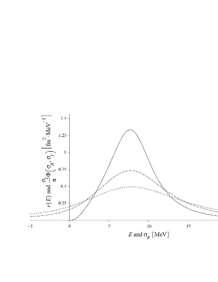
Figure 1: Full line: the response function $r(E)$. Dashed line: its integral transform $\Phi(\sigma_{R},\sigma_{I})$ at $\sigma_{I}=2.5$ MeV multiplied by $\sigma_{I}/\pi$. Dotted line: the same for $\sigma_{I}=5$ MeV.

IV Inversion of the LIT

When solving Eq. (9) we, as usual, seek for the response function in the form of an expansion over a set of basis functions $f_{n}(E;\alpha)$ where $\alpha$ is a fall–off parameter,

$$r(E)=\sum_{n=1}^{N}C_{n}f_{n}(E;\alpha).$$ (14)

Substitution of this expression in the right–hand side of Eq. (9) gives the trial transform $\Phi_{tr}$,

$$\Phi_{tr}(\sigma_{R},\sigma_{I})=\sum_{n=1}^{N}C_{n}{\bar{f}}_{n}(\sigma_{R},\sigma_{I};\alpha),$$ (15)

$${\bar{f}}_{n}(\sigma_{R},\sigma_{I};\alpha)=\int_{0}^{\infty}dE\,\frac{f_{n}(E;\alpha)}{(E-\sigma_{R})^{2}+\sigma_{I}^{2}}.$$ (16)

One imposes the minimum condition

$$\sum_{i}[\Phi((\sigma_{R})_{i},\sigma_{I})-\Phi_{tr}((\sigma_{R})_{i},\sigma_{I})]^{2}W(i)={\rm min}.$$ (17)

The minimization is performed with respect to the $C_{n}$ and $\alpha$ parameters entering $\Phi_{tr}$ on a sufficiently dense grid $(\sigma_{R})_{i}$ in some range of $\sigma_{R}$ values. The quantity $W(i)$ is a weight function. The condition (17) leads to the set of linear equations for the $C_{n}$ parameters.

In the exact arithmetic the inversion results would not depend on the choice of the mentioned range of $\sigma_{R}$ values since both sides of Eq. (9) are analytic functions of $\sigma_{R}$. However, in practice this choice matters. In Ref. suz it was recommended to employ a very wide range of these values, such that provides the fulfillment of the relation (11). We believe that such a choice is not an optimal one. Indeed, at such a choice much weight is given to the large $|\sigma_{R}|$ wings of $\Phi(\sigma_{R},\sigma_{I})$. But, in accordance with Eqs. (9) and (12), $\Phi(\sigma_{R},\sigma_{I})$ behaves at these wings as $\langle\rho^{2}\rangle/(\sigma_{R})^{2}$, i.e. in a universal way, and thus does not provide substantial information on the behavior of $r(E)$.

The choice of the range of $\sigma_{R}$ values for the inversion purposes is to be related with the interval $0\leq E\leq E_{max}$ of $E$ values on which we want to get the $r(E)$ response. Below we employ the $-2\sigma_{I}\leq\sigma_{R}\leq E_{max}+2\sigma_{I}$ range to this aim.

In Ref. suz the following basis set has been used,

$$f_{n}(E;\alpha)=E^{3}e^{-\alpha E/n}.$$ (18)

Below we shall perform the inversion in two versions. In one of them, we shall use exactly the same set (18). In the other version, we shall modify this set which will lead to simplifications.

As to the choice of the set (18), one may note that inversion is frequently facilitated by incorporating the true low–energy behavior of the response into the basis functions. In the case of two fragments above the threshold with no Coulomb inter–fragment interaction this behavior is $E^{l_{1}+1/2}$ which is seen from Eq. (4). The $E^{3}$ factor in Eq. (18) reproduces this behavior. The set of basis exponentials from Eq. (18) is complete in the sense of both $L^{2}(0,\infty)$ and $C(0,\infty)$ norms. This follows from the Münz theorem, see e.g. Akh .

The accuracy of inversion should increase as the number $N$ of basis functions in the expansion (14) increases. As in the previous work, see e.g. rev , stability of the results of the inversion in some range of $N$ values serves as a criterion of its reliability. However, as it is known, stability arising with an increase of $N$ may well be violated at its further increase due to the fact that not an exact transform but an approximate one is fitted. Besides, with the basis functions of Eq. (18) it is impossible to perform calculations at too large $N$ values because of round–off errors, see below.

We shall study the $\sigma_{I}=5$ MeV and $\sigma_{I}=2.5$ MeV cases. The first of these cases was considered in Ref. suz . Such choices of the $\sigma_{I}$ values would be reasonable when one deals with responses having widths comparable with that of the present $r(E)$ response. Use of smaller $\sigma_{I}$ values in the many–body case would require more effort in order to solve the inhomogenous equation like Eq. (7) with the same accuracy.

Inversion with the basis set (18) occurs to be the most difficult in the region of small energy. While in Ref. suz the weight function $W(i)$ entering the fitting procedure of Eq. (17) was taken to be unity, here, to improve the inversion in the mentioned region in the case of set (18), $W(i)$ has been chosen as follows. Below the point $\sigma_{R}=\sigma_{0}$ of the maximum, at a given $\sigma_{I}$, of $\Phi(\sigma_{R},\sigma_{I})$ the weight function $W(i)$ was taken to be $[\Phi(\sigma_{0},\sigma_{I})/\Phi((\sigma_{R})_{i},\sigma_{I})]^{2}$ and it was taken to be unity beyond this point.

Even at this choice of $W(i)$ it is necessary to retain rather many basis functions (18) in Eq. (14) to get a good inversion at small energy. It occurs that when the number of basis functions increases the expansion coefficients become very large in magnitude. In the present case they reached the values about $10^{10}$ at the highest $N$ values we employed. Corresponding contributions strongly cancel each other. This feature has not been noticed so far. Because of it, the inversion was performed via calculations with the quadrupole precision in this version. Also the integrals (16) are to be calculated here with high accuracy. They were expressed nir in terms of the incomplete gamma function of a complex argument. However, the accuracy with which this function is provided by existing codes is not known. We calculated these integrals numerically in the intervals $0\leq E\leq E_{max}$ at $E_{max}=130n/\alpha$ MeV with the relative accuracy of $10^{-21}$. All this provided sufficient stability of the final results at $E\geq 3$ MeV. However, at lower energies the stability remains incomplete irrespective to accuracy of the integration. At $\sigma_{I}=5$ MeV round–off errors may influence the result in the first non–zero decimal place at $E=1$ MeV and in the second non–zero decimal place at $E=2$ MeV. At $\sigma_{I}=2.5$ MeV they may influence the result in the second non–zero decimal place at $E=1$ MeV and in the third non–zero decimal place at $E=2$ MeV.

Provided that the overlap integrals of basis functions are known exactly, as in the present case, it is probably possible to get rid of the large $|C_{n}|$ values using a basis set $f_{n}$ in Eq. (14) which is orthonormalized. In this case, the $C_{n}$ coefficients for the corresponding expansion of the exact $r(E)$ are such that the sum $\sum_{n=1}^{N}C_{n}^{2}$ is bounded from above by the integral from $r^{2}(E)$ over all the energies. Therefore, the $|C_{n}|$ values cannot be large. Probably this refers also to the approximate $C_{n}$ coefficients determined from the fit. However, this version have not been tried.

In the above version of the calculation, the optimal value of the $\alpha$ parameter entering functions (18) was searched first on a grid. After that, the minimum of the expression (17) was looked for on a smaller $\alpha$ interval. However, at large $N$ values the arising dependence of the quantity (17) on $\alpha$ becomes a fluctuating one due to a strong cancellation between $\Phi$ and $\Phi_{tr}$. Because of this, it is not possible to find the absolute minimum. Anyway, the obtained fits to $\Phi(\sigma_{R},\sigma_{I})$ are very precise.

Table 5: The exact response $r(E)$ and the responses obtained via inverting the LIT of $r(E)$ at $\sigma_{I}=5$ MeV with various numbers $N$ of basis functions retained in the expansion (14). The energy $E$ is in MeV.

		$N$
$E$	exact	30	35	40	45	50
1	0.044	-0.042	0.012	0.015	0.009	0.005
2	0.177	0.215	0.178	0.196	0.198	0.237
3	0.354	0.361	0.363	0.357	0.356	0.349
4	0.564	0.559	0.559	0.561	0.562	0.564
8	1.321	1.322	1.321	1.321	1.321	1.322
12	0.452	0.452	0.452	0.452	0.452	0.452
16	0.130	0.130	0.130	0.130	0.130	0.130
20	0.048	0.048	0.048	0.048	0.048	0.048

In Table V the results of the above described inversions at $\sigma_{I}=5$ MeV are presented at some energies $E$ and various numbers $N$ of basis functions retained in the expansion (14). The exact response $r(E)$ is presented in the second column and the responses obtained from the inversion of the LIT are shown in columns from three to seven. Note that at $E\geq 4$ MeV at least the two–digit accuracy of inversion has been obtained also for all the $E$ values not shown in the Table in the range $E\leq 20$ MeV considered. As to lower energy, the results are also rather accurate at $E=3$ MeV, and at $E=2$ MeV they are of a moderate accuracy. These results are different from those of Ref. suz where large or substantial deviations from the true response were found at all the energies.

In Table VI the corresponding results at $\sigma_{I}=2.5$ MeV are presented. The results in the range considered for energies not presented in the table are quite similar. Here we show also the results of the inversions at smaller $N$ values which deviate from those in the region of stability with respect to $N$. In this case, stability is reached at $N$ values smaller than in the preceding $\sigma_{I}=5$ MeV case. It is also seen that in the present case stability takes place also at small energies. This is in line with the fact that the resolution of the Lorentz kernel here is higher than in the preceding case.

Table 6: The exact response $r(E)$ and the responses obtained via inverting the LIT of $r(E)$ at $\sigma_{I}=2.5$ MeV. The notation is as in Table V.

		$N$
$E$	exact	10	15	20	23	25	27	28
1	0.044	0.107	0.113	0.029	0.044	0.044	0.041	0.043
2	0.177	0.118	0.158	0.167	0.186	0.183	0.176	0.184
3	0.354	0.390	0.358	0.362	0.355	0.355	0.356	0.355
4	0.564	0.571	0.561	0.560	0.563	0.563	0.563	0.563
8	1.321	1.311	1.321	1.321	1.321	1.321	1.321	1.321
12	0.452	0.454	0.452	0.452	0.452	0.452	0.452	0.452
16	0.130	0.131	0.130	0.131	0.131	0.131	0.130	0.131
20	0.048	0.048	0.049	0.049	0.049	0.049	0.048	0.049

It should be noted that the above precise calculations were feasible solely due to the fact that the input transform was known with a high precision. In the usual many–body applications one works with a transform that is considerably less precise than in the present case. In what follows a simpler version of the inversion is presented. As we shall see, in this case so high a precision of the calculation is not required. Accordingly, for the inversions that follow we use an upper integration limit of 100 MeV in Eq. (17) (tiny contributions beyond 100 MeV are neglected). The weight function $W(i)$ is taken to be unity. In addition a sowewhat different search for the fall-off parameter $\alpha$ is implemented. For a predefined set of $\alpha$ values the minimization of Eq. (17) is performed with respect to the linear parameters $C_{n}$. For any number of basis functions $N$ the parameter set leading to the smallest value of Eq. (17) is taken. Note that the response function is positive definite, therefore we exclude parameter sets that lead to a negative response in the energy interval of interest. The interval of $\sigma_{R}$ values we consider here runs from zero up to $E_{max}+2\sigma_{I}$.

The search for an optimal $\alpha$ value is made as follows. We run $\alpha$ over a large grid of possible values and determine the error given by the left-hand side of Eq. (17). In the present case the search was made with the following values:

$$\alpha(j)={\frac{1000}{j}}$$ (19)

with $j=1,2,...,1500$. We select the best fit among the 1500 trials as inversion result, which, in addition, has to fulfil the above defined positiveness condition.

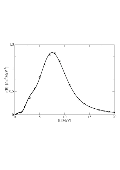
Figure 2: Inversion results for $N$ ranging from 10 to 20 ($\sigma_{I}=5$ MeV). Any of the eleven inversions is represented by a solid line, true response is depicted by crosses (x).

After having determined the ”best” response functions for the various number of basis functions one compares the obtained results. In a perfect inversion of an analytically known transform $\Phi$ the precision of the inversion improves with a growing number $N$ of basis functions. In practise, due to numerical errors both in the calculation of $\Phi$ and in the inversion, one should observe a scenario already described above after Eq. (18): With an increase of $N$ one should find a rather stable inversion result for a limited range of $N$ values, then, with a further increase of $N$ the stability is lost.

In Fig. 2 we show the inversion results for the $\sigma_{I}=5$ MeV case, where $N$ runs from 10 to 20. One observes a rather stable result, in fact inversions with $15\leq N\leq 20$ are almost identical. Unsatisfying is the somewhat oscillatory behaviour below 5 MeV. In fact comparing with the true response one finds differences up to the peak region.

One can try to improve the inversion using a smaller $\sigma_{I}$ value. Taking $\sigma_{I}=2.5$ MeV we obtain very stable inversion results with $N=15,16,17$, whereas for even higher $N$ stronger low-energy oscillations set in. In Fig. 3 we compare these results with the stable result obtained for $\sigma_{I}=5$ MeV. The comparison is made only at lower energies, since at higher energies results are almost identical. For $\sigma_{I}=2.5$ MeV one notes a reduction of the oscillatory low-energy behaviour with an improvement of the result, particularly visible at 3 and 5 MeV.

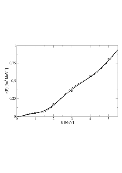
Figure 3: Comparison of inversion results with $\sigma_{I}=2.5$ MeV (solid line) and $\sigma_{I}=5$ MeV (dotted line). Crosses (x) as in Fig. 2.

Thus, in order to further improve the quality of the inversion one should work with a considerably smaller $\sigma_{I}$. In general, it is not easily possible to calculate the transform $\Phi$ with a sufficient precison for a much smaller $\sigma_{I}$. However, even in the present case a further improvement can be made. As already stated the inversions show an oscillatory behaviour at lower energies. This points in the direction that the chosen basis set is not very efficient. To illustrate this better we show in Fig. 4 the inversion result for $\sigma_{I}=2.5$ MeV and $N=8$. One observes that there is a maximum at about 0.6 MeV and a minimum at about 1.2 MeV. Such a structure of the response at threshold is rather improbable and in fact for the above mentioned stable inversion result with $N=15,16,17$ such a strong low-energy oscillation has vanished. To avoid a fake strong low-energy rise one can take a different low-energy behaviour of the basis functions used for the inversion. In this connection one may note that in reality the $E^{3}$ behavior of the response takes place only in a quite narrow energy region close to zero. Deviations from this behavior are large already at e.g. $E=0.2$ MeV. (But if one drops all the oscillator basis functions except the lowest one in the expansion obtained of the bound state wave function then the $E^{3}$ behavior of the spectrum will take place in a rather wide range of energy. With the five percent accuracy it is then valid up to energies higher than $E=1$ MeV.)

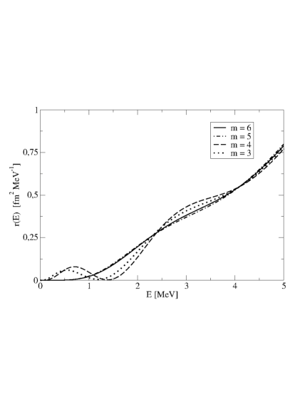
Figure 4: Inversions for $\sigma_{I}=2.5$ MeV and $N=8$ for various sets of basis functions, $f_{n}(E;\alpha,m)=E^{m}e^{-\alpha E/n}$, with $m=3,4,5,6$.

In Fig. 4 we also show results where the low-energy rise of $E^{3}$ of the $f_{n}$ of Eq. (18) is changed into $E^{m}$ with $m=4,5,6$. One sees that the unwanted low-energy behaviour goes away with $m=5,6$. Studying better the case with $m=6$ we find a stable inversion with $N=14,15,16$. The corresponding results are shown in Fig. 5. Now one observes a very nice agreement between true response and inversion result also at low energies.

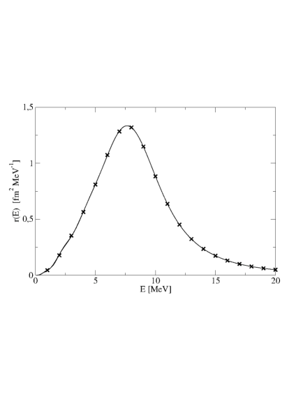
Figure 5: Inversions for $\sigma_{I}=2.5$ MeV and $N=14,15,16$ (solid lines) with basis function sets $f_{n}(E;\alpha,m=6)$. Crosses (x) as in Fig. 2.

V summary

In Ref. suz the question was addressed whether the response function provided by the model of that work may be obtained with a resonable accuracy via inverting its LIT calculated with the bound–state type method. The answer proved to be negative. In the present work, the problem was reconsidered and, at variance with the results of Ref. suz , accurate approximations to the true response have been obtained with that method.

Our calculation differs from that of Ref. suz both in its input and in the inversion procedure. As to the input, the LIT calculated from the inhomogeneous equation in the present work proves to be different from that in Ref. suz . Also the ranges of values of the transform employed for the inversion have been chosen differently.

We started with the same inversion procedure as in Ref. suz except for the weight function used at fitting the transform. In particular, the basis set used at performing the inversion was the same. In this way we succeeded to obtain the responses of an acceptable accuracy. Rather many basis functions were to be retained in order to reach the inversion stability at low energy.

However, transforms pertaining to few–body calculations normally have considerably lower accuracy than in the present case. To invert them, use of such an amount of basis functions is not possible since the stability of inversion results would then be lost and a non–physical oscillating function would be selected in the course of the inversion as the output response.

The next variant of our inversion procedure was the following. The response function that provides the best fit to an input transform is selected in the course of the inversion. We imposed the condition that response functions taking non–physical negative values are discarded at searching for the best fit. At this condition, the stability of the inversion results has been reached at lower numbers of basis functions than above. The responses obtained still exhibit somewhat oscillatory behavior at low energy.

Finally, we have modified the basis set used for the inversion. The inital basis set reproduced the low–energy behavior of the true response. Such a condition was usually imposed in calculations in the literature and seemed to improve ELO99 the inversion results. However, in the present case this proved to be not true and just because of this condition it was necessary to retain a large amount of basis functions in the first above mentioned variant of the inversion procedure. The peculiarity of the present problem is that the asymptotic low–energy behavior of the response takes place only in a very limited energy range. Therefore, we have modified the factor entering the basis functions which describes the low–energy behavior of the response sought for. We have chosen this factor from the condition that non–physical oscillations of the response are excluded already at small number of basis functions used for the inversion. This improved our outcome at low energy leading to a nice agreement between the inversion result and the true response.

Acknowledgement of support is given to RFBR Grant No. 18–02–00778 (V.D.E and V.Yu.S.).

References

- (1) V. D. Efros, W. Leidemann, and G. Orlandini, Phys. Lett. B338 130, (1994).
- (2) V.D. Efros, W. Leidemann, G. Orlandini, and N. Barnea, J. Phys. G: Nucl. Part. Phys. 34, R459 (2007).
- (3) Y. Suzuki, W. Horiuchi, and D. Baye, Progr. Theor. Phys. 123, 547 (2010).
- (4) V.D. Efros, W. Leidemann, and G. Orlandini, Few Body Syst. 26, 251 (1999).
- (5) V.D. Efros, Phys. At. Nucl. 62, 1833 (1999) (arXiv:nucl-th/9903024).
- (6) C. Reiss, E.L. Tomusiak, W. Leidemann, and G. Orlandini, Eur. Phys. J. A17, 589 (2003).
- (7) N. Barnea and E. Livertz, Few Body Syst. 48, 11 (2010).
- (8) W. Leidemann, Few Body Syst. 42, 139 (2008).
- (9) W. Leidemann, Phys. Rev. C 91, 054001 (2015).
- (10) W. Leidemann, S. Deflorian, and V.D. Efros, Few Body Syst. 58: 27 (2017); S. Deflorian, V.D. Efros, and W. Leidemann, Few Body Syst. 58: 3 (2017).
- (11) W. Glöckle and M. Schwamb, Few Body Syst. 46, 55 (2009); N. Barnea, V.D. Efros, W. Leidemann, and G. Orlandini, Few Body Syst. 47, 201 (2010).
- (12) V.D. Efros, Phys. Rev. E 86 016704 (2012).
- (13) D. Andreasi, W. Leidemann, C. Reiss, and M. Schwamb, Eur. Phys. J. A24, 361 (2005).
- (14) W.H. Press, S.A. Teukolsky, W.T. Weterling, and B.P. Flannery, Numerical Recipes (Cambridge University Press 1997).
- (15) M.V. Zhukov and V.D. Éfros, Yad. Fiz. 14, 577 (1971) [Sov. J. Nucl. Phys. 14, 322 (1972)]; V.D. Efros, Phys. Rev. C (in press).
- (16) N.I. Achieser, Theory of Approximation (Dover, N.Y. 2003).