Do Hertzsprung-Gap Stars Show Any Chemical Anomaly?

Abstract

With an aim to investigate how the surface abundances of intermediate-mass stars off the main sequence (evolving toward the red-giant stage) are affected by the evolution-induced envelope mixing, we spectroscopically determined the abundances of Li, C, N, O, and Na for selected 62 late A through G subgiants, giants, and supergiants, which are often called “Hertzsprung-gap stars,” by applying the synthetic spectrum-fitting technique to Li i 6708, C i 5380, N i 7460, O i 6156–8, and Na i 6161 lines. A substantially large star-to-star dispersion ($\gtrsim 2$ dex) was confirmed for the Li abundances, indicating that this vulnerable element can either suffer significant depletion before the red-giant stage or almost retain the primordial composition. Regarding C, N, O, and Na possibly altered by dredge-up of nuclear-processed products, their abundances turned out to show considerable scatter. This suggests that these abundance results are likely to suffer appreciable uncertainties, the reason for which is not clear but might be due to some kind of inadequate modeling for the atmospheric structure. Yet, paying attention to the fact that the relative abundance ratios between C, N, and O should be more reliable (because systematic errors may be canceled as lines of similar properties are used for these species), we could confirm a positive correlation between [O/C] (ranging from $\sim 0$ to $\sim+0.5$ dex) and [N/C] (showing a larger spread from $\sim 0$ to $\sim+1$ dex), which is reasonably consistent with the theoretical prediction. This observational detection of C deficiency as well as N enrichment in our program stars manifestly indicates that the dredge-up of H-burning product can take place before entering the red-giant stage, with its extent differing from star to star.

1 Introduction

Stars leave off the main sequence after the hydrogen fuel in the core has been exhausted and evolve toward the red giant stage with a progressive lowering of the surface temperature; i.e., from left to right on the Hertzsprung–Russell (HR) diagram. Since the deepening of convention zone takes place during this course, some H-burning product in the core may be salvaged to the surface if the envelope mixing penetrates sufficiently deep, by which characteristic chemical anomalies would be observed. Actually, such signs of abundance peculiarities (e.g., C deficit or Na enrichment as a result of contamination by CN- or NeNa-cycle product) are actually observed in red giant stars (see, e.g., Takeda et al. 2015 and the references therein).

However, it has not yet been well understood how much and when such mixing-induced dredge-up actually occurs. According to the theoretical prediction considering only the classical convective mixing (canonical theory of first dredge-up), observable abundance anomalies do not appear until a star has entered the red giant phase with sufficiently low $T_{\rm eff}$ ($\lesssim 5000$ K). Yet, such a conventional theory does not seem to be sufficient and other type of additional mixing mechanism is likely to exist in the envelope of actual stars. For example, the mixing induced by rotation (e.g., meridional circulation or rotational shear instability) may contribute to a significant dredge-up, which appears to take place already in the main-sequence phase for the case of rapidly-rotating B-type stars as seen from their surface He enrichment (Lyubimkov et al. 2004). Therefore, recent extensive calculations such as done by Lagarde et al. (2012) tend to make practice of including non-canonical mixing (rotational as well as thermohaline mixing) in simulating the surface abundance changes during the course of stellar evolution.

Even so, we are not sure whether such a more sophisticated modeling with non-canonical mixing is really superior to the simple classical theory. For example, Anthony-Twarog et al. (2018) reported based on their Li abundance study of 287 low-to-intermediate mass stars in the open cluster NGC 2506 that the observed abundance trend agrees with the prediction from theoretical models including rotational+thermohaline mixing. On the other hand, Smiljanic et al. (2018) argued in their spectroscopic investigation on the C, N, O, Na, and Al abundances of 20 intermediate-mass red giants in 10 open clusters that models with rotational mixing tend to overestimate the mixing effects and thus not preferable.

Given the situation being still unsettled as such, it is important in the first place to accumulate more observational data concerning the abundances of light elements (possibly influenced by mixing) for as many evolved stars as possible. Generally speaking, however, previous abundance studies in this field tended to focus rather on well-evolved low/intermediate-mass red giants of late G or K type, which were B–A–F stars when they were on the main sequence. If we are to investigate how the surface abundances undergo changes in the course of stellar evolution off the main sequence, it is necessary to pay attention also to stars on the mid-way between early-type dwarfs and late-type giants. Such stars (typically late A through early G giants or supergiants) are generally few in number, because they are evolving quite rapidly towards the right (cooler) direction on the near-horizontal tracks and thus the probability of being found by us small. Accordingly, we can recognize a void-like region of low star density in the HR diagram, which is occasionally called “Hertzsprung gap.”

Some number of studies regarding the chemical abundances of light elements in Hertzsprung-gap stars have been published so far, which we briefly summarize as follows (though not meant to be complete): Luck & Lambert (1985) discussed the CNO abundances of F-type supergiants and Cepheids in connection with the nature of envelope mixing. Takeda & Takada-Hidai (1994) investigated the behavior of Na abundances in A–F supergiants (including some Cepheids). Barbuy et al. (1996) determined the CNO abundances of 9 yellow F-type supergiants to see if any mixing-related anomaly exists. Successively, Smiljanic et al. (2006) reported the CNO abundances of 19 late A through early K giants and supergiants. Lyubimkov et al. (2011) determined the N abundances of 30 A- and F-type supergiants and discussed the nature of N-enrichment process. Takeda et al. (2013) carried out a comprehensive analysis on the C, N, O, and Na abundances of 12 Cepheid variables. Adamczak & Lambert (2014) examined the C and O abundances for 188 stars across the Hertzsprung gap, which is probably the most extensive investigation as far as the number of sample stars is concerned. Molina & Rivera (2016) reported the chemical abundances of many elements (including C, N, O, and Na) in 4 A–F supergiants.

In spite of these investigations, however, the picture of evolution-induced chemical anomaly in this group of stars has not been clarified yet. Besides, targets in these past studies, except for Adamczak & Lambert (2014), appear to be biased toward comparatively slow rotators, despite rapid rotators are commonly included in this group of stars (presumably because of the growing difficulty in abundance determinations).

Given this circumstance, we decided to challenge this task, taking advantage of the results and experiences in our recent studies:
— Regarding the observational data, the high-dispersion spectra of 75 evolved A-, F-, and G-type stars in the Hertzsprung-gap region are already available, which we used for investigating the luminosity effect of O i 7771–5 triplet lines (Takeda et al. 2018a; hereinafter referred to as Paper I). Besides, the atmospheric parameters of these stars (including the microturbulence which is not easy to determine for broad-line stars) have already been established in Paper I.
— As to the surface chemical composition of red giants (into which Hertzsprung-gap stars will further evolve sooner or later), Takeda et al. (2015) reported the abundances of C, O, and Na for 239 late G through early K giants. Likewise, Takeda et al. (2013) investigated the C, N, O, and Na abundances of 12 Cepheid variables, which may also be used for comparison.
— On the other hand, surface C, N, and O abundances of late B through early F dwarfs (from which $\sim$ 1.5–5 $M_{\odot}$ stars currently in the Hertzsprung gap have evolved) have recently been investigated in detail by Takeda et al. (2018c; hereinafter referred to as Paper II).
— Since these previous studies made use of the spectrum synthesis technique, which is indispensable for deriving the elemental abundances of rapid rotators often included in Hertzsprung-gap stars, we may be able to compare the abundances of different star groups in a consistent manner by applying the same method of analysis.

Accordingly, we investigated in this study the abundances of representative light elements (Li, C, N, O, and Na, which may be affected by evolution-induced mixing) for selected 62 Hertzsprung-gap stars (late A through G subgiants, giants, and supergiants) by making use of the observational data adopted in Paper I. Here, we particularly intended to examine the following points of interest.

• Do these stars currently evolving across the Hertzsprung gap show abundance anomalies typically seen in red giants or Cepheids (e.g., underabundance in C, overabundance in N or Na)? If really observed, is there any meaningful dependence upon the stellar parameters (e.g., $T_{\rm eff}$ or $M$)?

• How are the abundances of these evolved stars compared with low-mass (FGK) dwarfs covering wide range of stellar ages? Meanwhile, do they show any relation with the C, N, and O deficiencies observed in A-type dwarfs (most likely caused by the diffusion process and confined only to the surface layer)?

2 Program stars and their parameters

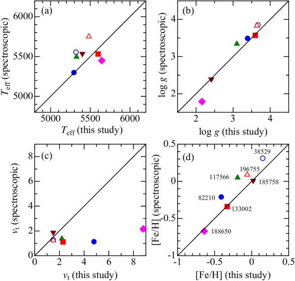
Figure 2: Comparison of the stellar parameters adopted in this study (taken from Paper I) with those determined spectroscopically based on Fe i and Fe ii lines by Takeda et al. (2005) (open symbols for 2 stars in common: HD 38529 and 196755) and Takeda et al. (2008) (filled symbols for 5 stars in common: HD 82210, 117566, 133002, 185758, and 188650). (a) $T_{\rm eff}$, (b) $\log g$, (c) $v_{\rm t}$, and (d) [Fe/H].

Among the 75 stars investigated in Paper I, the effective temperatures of early A-type supergiants tend to suffer appreciably larger ambiguities (cf. Fig. 2a therein), mainly because of the considerable interstellar extinction (due to their distant nature with low galactic latitude). Accordingly, we decided to discard 13 stars (those with $T_{\rm eff}>8500$ K or classified as early A supergiants), which eventually resulted in 62 program stars, as listed in Table 1. See Sect. 2 in Paper I for the description of the observational data of these targets, which were obtained with the echelle spectrograph attached to the 1.8 m reflector at Bohyunsan Astronomical Observatory.

Regarding $T_{\rm eff}$ (effective temperature; from $B-V$ colors) and $\log g$ (surface gravity; from luminosity with the help of evolutionary tracks), we used the same values as derived in Paper I (cf. Sect. 3 therein). As to the microturbulence ($v_{\rm t}$), we adopted the values determined in Paper I by requiring the abundance consistency between O i 7771–5 and O i 6156–8 lines (denoted as $\xi_{\rm a}$; cf. Sect. 6 therein) wherever possible. In case that $\xi_{\rm a}$ could not be determined in Paper I, we used the alternative microturbulence ($\xi_{\rm p}$) determined from the line profile of O i 7771–5 triplet (cf. Sect. 5 therein). The model atmosphere assigned to each star is described in Sect. 4 of Paper I.

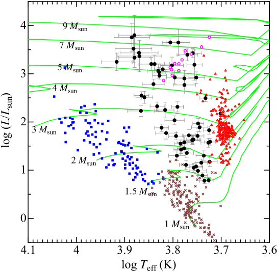
Figure 1: Our 62 program stars are plotted on the $\log(L/L_{\odot})$ vs. $\log T_{\rm eff}$ diagram by filled circles with error bars (see the caption of Fig. 1 in Paper I for their derivation). In addition, the targets studied in Takeda & Honda (2005) (160 F–G–K dwarfs), Takeda et al. (2013) (12 F–G Cepheids), Takeda et al. (2015) (239 G–K giants), and Paper II (100 A-type dwarfs) are also shown for comparison by crosses, open circles, open triangles, and filled squares, respectively. Depicted in solid lines are the theoretical solar-metallicity tracks computed by Lejeune and Schaerer (2001) for 8 different masses (1, 1.5, 2, 3, 4, 5, 7, and 9 $M_{\odot}$).

The $\log L$ vs. $\log T_{\rm eff}$ plots of our 62 Hertzsprung-gap stars are shown in Fig. 1, where the relevant targets of different star groups (red giants, Cepheids, main-sequence stars) studied in our previous papers are also depicted. Similarly, $\log g$, $v_{\rm t}$, and $v_{\rm e}\sin i$ (projected rotational velocity determined from 6145–6166 Å fitting described in Sect. 3.1) for each star are plotted against $T_{\rm eff}$ and $M$ (stellar mass) in Fig. 2. We can see from these figures that our sample stars cover the parameter ranges of 8000 K $\gtrsim T_{\rm eff}\gtrsim 5000$ K, 1.8 $\lesssim\log g\lesssim$ 3.7, $1.5M_{\odot}\lesssim M\lesssim 8M_{\odot}$, 0 km s${}^{-1}\lesssim v_{\rm t}\lesssim 10$ km s^-1, and 0 km s${}^{-1}\lesssim v_{\rm e}\sin i\lesssim 150$ km s^-1.

As for the error bars ($\sigma$) attached to the data points in Fig. 1 and Fig. 2, $\sigma(T_{\rm eff})$’s are due to ambiguities of interstellar reddening, $\sigma(\log L)$’s are evaluated by combining the uncertainties of interstellar extinction and of Hipparcos parallax, $\sigma(M)$’s are due to ambiguities in $L(\propto M^{4})$, and $\sigma(\log g)$’s are estimated from $\sigma(T_{\rm eff})$ and $\sigma(L)$ (where we formally assume that both are independent and that random errors in $M$ are comparatively insignificant and negligible). The adopted stellar parameters for each program star are summarized in Table 1 (and in “tableE.dat” of the online material where their errors are also given).

3 Abundance determinations

Given that our task is to study the surface abundances of Li, C, N, O, and Na for 62 Hertzsprung-gap stars, we invoke Li i 6708, C i 5380, O i 6156–8, N i 7468, and Na i 6161 lines as in Takeda & Tajitsu (2017) (for Li, C, O, Na) and Paper II (for C, N,and O). The determination procedures of abundances and related quantities (e.g., non-LTE correction, uncertainties due to ambiguities of atmospheric parameters) are essentially the same as described in these papers, which consist of two consecutive steps.

3.1 Synthetic spectrum fitting

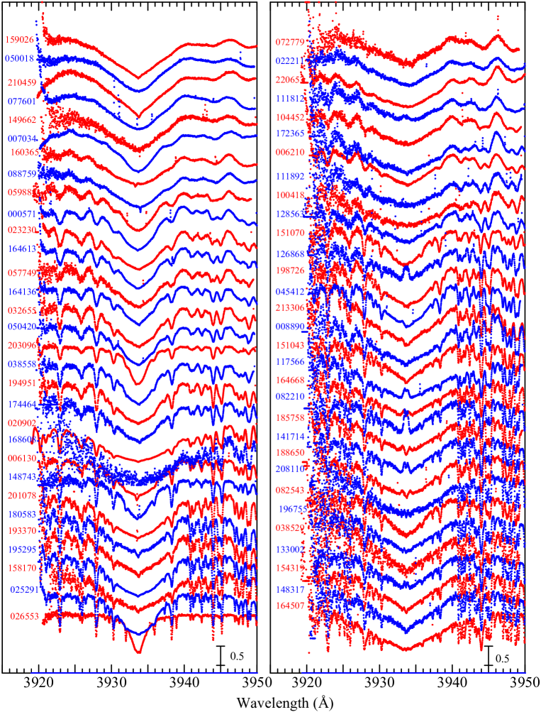
Figure 3: Display of the spectra in the 3920–3950 Å region (comprising the Ca ii K line at 3933.663 Å) for the 62 program stars, which are arranged according to the decreasing order of $v_{\rm e}\sin i$ as in Fig. 3 (left panel: $T_{\rm eff}>6000$ K, right panel: $T_{\rm eff}<6000$ K). Each spectrum, tentatively normalized at $\sim$ 3946 Å, is vertically shifted by 0.5 relative to the adjacent one. The wavelength scale is adjusted to the laboratory frame by correcting the radial velocity shifts. The HD numbers are indicated in the figure.

The first step is to find the solutions for the abundances of relevant elements ($A_{1},A_{2},\ldots$), projected rotational velocity ($v_{\rm e}\sin i$), and radial velocity ($V_{\rm rad}$) by requiring the best fit (minimizing $O-C$ residuals) between theoretical and observed spectra, while applying the automatic fitting algorithm (Takeda 1995a). Four wavelength regions were selected for this purpose: (i) 6702–6714 Å region (for Li), (ii) 5370–5390 Å region (for C), (iii) 7457–7472 Å region (for N), and (iv) 6145–6166 Å region (for O, Na). More information about this fitting analysis (varied elemental abundances, used data of atomic lines) is summarized in Table 2. How the theoretical spectrum for the converged solutions fits well with the observed spectrum is displayed in Fig. 3–6 for each region. The $v_{\rm e}\sin i$ values resulting from the fitting of 6145–6166 Å region are presented in Table 1. We also adopted the solution of Fe abundance derived from the fitting of 6146–6163 Å region as the metallicity of each star (given as [Fe/H] in Table 1).

3.2 Abundances from equivalent widths

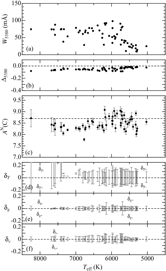
Figure 8: Carbon abundance and C i 5380-related quantities plotted against $T_{\rm eff}$. The reference C abundance of $A^{\rm N}$(C:Procyon) = 8.70 is indicated by the horizontal dashed line in panel (c). Otherwise, the same as in Fig. 7.

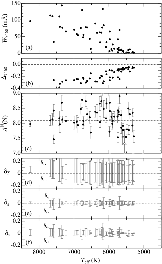
Figure 9: Nitrogen abundance and N i 7486-related quantities plotted against $T_{\rm eff}$. The reference N abundance of $A^{\rm N}$(N:Procyon) = 8.10 is indicated by the horizontal dashed line in panel (c). Otherwise, the same as in Fig. 7.

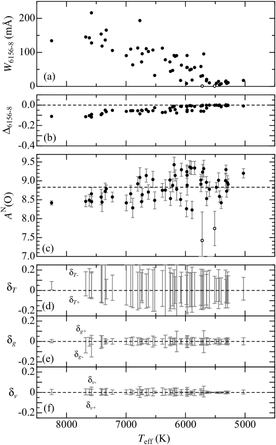
Figure 10: Oxygen abundance and O i 6156–8-related quantities plotted against $T_{\rm eff}$. The reference O abundance of $A^{\rm N}$(O:Procyon) = 8.83 is indicated by the horizontal dashed line in panel (c). Otherwise, the same as in Fig. 7.

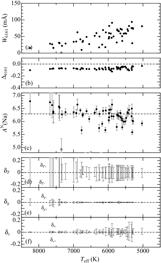
Figure 11: Sodium abundance and Na i 6161-related quantities plotted against $T_{\rm eff}$. The reference Na abundance of $A^{\rm N}$(Na:Procyon) = 6.29 is indicated by the horizontal dashed line in panel (c). Otherwise, the same as in Fig. 7.

As the second step, with the help of Kurucz’s (1993) WIDTH9 program (which had been considerably modified in various respects; e.g., inclusion of non-LTE effects, treatment of total equivalent width for multi-component lines; etc.), we computed the equivalent widths ($W$) of the representative lines “inversely” from the abundance solutions (resulting from spectrum synthesis) along with the adopted atmospheric model/parameters; i.e., $W_{6708}$ (for Li i 6708), $W_{5380}$ (for C i 5380), $W_{6156-8}$ (for O i 6156–8), $W_{7468}$ (for N i 7468), and $W_{6161}$ (for Na i 6161), which are easier to handle in practice (e.g., for estimating the uncertainty due to errors in atmospheric parameters). The adopted atomic data for these lines are summarized in Table 3. We then analyzed such derived $W$ values by using WIDTH9 to determine $A^{\rm N}$ (NLTE abundance) and $A^{\rm L}$ (LTE abundance), from which the NLTE correction $\Delta(\equiv A^{\rm N}-A^{\rm L})$ was further derived. We adopted Procyon as the standard star of abundance reference (except for Li, which should be compared with the solar system abundance of 3.31 as done in Takeda & Tajitsu 2017), because it is known to have practically the same abundance as the Sun. We thus define the relative abundance as [X/H] $\equiv$ $A_{\rm X}^{\rm N}$(star) $-$ $A_{\rm X}^{\rm N}$(Procyon) (X = C, N, O, and Na). The references abundances of $A_{\rm X}^{\rm N}$(Procyon) (to be determined in the same manner and with the same atomic data as adopted in this study) are 8.70 (C), 8.10 (N), 8.83 (O), 6.29 (Na), and 7.47 (Fe), where those of C, N, O, and Fe were taken from Paper II and that of Na was newly determined in this study. The resulting values of $A^{\rm N}$(Li), [C/H], [N/H], [O/H], [Na/H] are given in Table 1 (more complete results including $W$ and $\Delta$ are separately presented in “tableE.dat”). Figs. 7(C), 8(C), 9(N), 10(O), and 11(Na) graphically show the equivalent width ($W$), non-LTE correction ($\Delta$), non-LTE abundance ($A^{\rm N}$), and abundance variations in response to parameter changes (see the following Sect. 3.3), as functions of $T_{\rm eff}$.

3.3 Error estimation

In order to evaluate the abundance errors caused by uncertainties in atmospheric parameters, we estimated six kinds of abundance variations ($\delta_{T+}$, $\delta_{T-}$, $\delta_{g+}$, $\delta_{g-}$, $\delta_{v+}$, and $\delta_{v-}$) for $A^{\rm N}$ by repeating the analysis on the $W$ values while perturbing the standard atmospheric parameters interchangeably by $\pm\sigma(T_{\rm eff)}$ (cf. Sect. 2), $\pm\sigma(\log g)$ (cf. Sect. 2), and $\pm\sigma(v_{\rm t})$ (which we tentatively assumed $\pm$max$[1.0,0.3v_{\rm t}]$ km s^-1 by consulting Fig. 10d in Paper I). Finally, the root-sum-square of these perturbations, $\delta_{Tgv}\equiv(\delta_{T}^{2}+\delta_{g}^{2}+\delta_{v}^{2})^{1/2}$, were regarded as the abundance uncertainties due to combined errors in $T_{\rm eff}$, $\log g$, and $v_{\rm t}$, where $\delta_{T}$, $\delta_{g}$, and $\delta_{\xi}$ are defined as $\delta_{T}\equiv(|\delta_{T+}|+|\delta_{T-}|)/2$, $\delta_{g}\equiv(|\delta_{g+}|+|\delta_{g-}|)/2$, and $\delta_{v}\equiv(|\delta_{v+}|+|\delta_{v-}|)/2$, respectively. These $\delta_{T\pm}$, $\delta_{g\pm}$, and $\delta_{v\pm}$ are plotted against $T_{\rm eff}$ in panels (d), (e), and (f) of Figs. 7–11, from which can generally state that $\delta_{T\pm}$ is most significant (which can be as large as $\sim 0.2$ dex or even more), while the other two are of comparatively minor importance.

We also evaluated errors in the equivalent width ($\delta W$) by assuming the typical S/N of $\sim 200$, from which the corresponding abundance uncertainties ($\delta_{W}$) were derived as done in Paper II (see Sect. 4.3 therein). Since $\delta W$ is quite small (typically several tenths to a few mÅ depending on $v_{\rm e}\sin i$), $\delta_{W}$ is only a few hundredths dex in most cases, except for the case of very weak lines where $\delta_{W}$ can be appreciably large as much as several tenths dex. Since the abundance results are regarded as unreliable if $W$ is smaller than 3$\delta_{W}$ (cf. Sect. 4.3 in Paper II), the relevant solutions of 3 stars (Li), 3 stars (N), 2 stars (O), and 1 star (Na) satisfying this criterion were discarded (these rejected data points are indicated by open circles in panels (a) and (c) of Figs. 7, 9, 10, and 11).

Finally, combining $\delta_{Tgv}$ and $\delta_{W}$, we evaluated the total error as $\delta_{TgvW}\equiv(\delta_{Tgv}^{2}+\delta_{W}^{2})^{1/2}$, which are shown as error bars attached to the non-LTE abundances in panel (c) of Figs. 7–11, though $\delta_{TgvW}$ is generally dominated by $\delta_{Tgv}$ (i.e., $\delta_{TgvW}\simeq\delta_{Tgv}$).

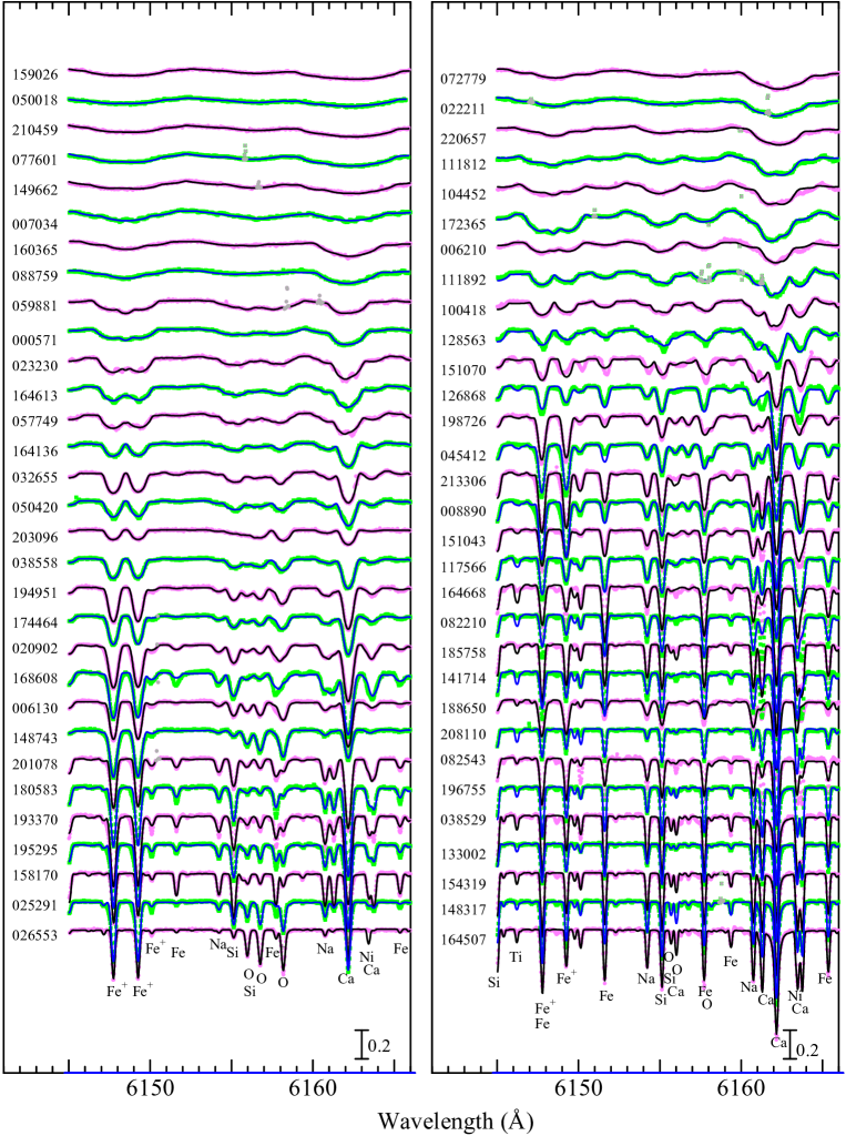
Figure 6: Synthetic spectrum fitting in the 6145–6166 Å region comprising the O i 6156–8 and Na i 6161 lines. A vertical offset of 0.2 is applied to each spectrum relative to the adjacent one. Otherwise, the same as in Fig. 3.

Meanwhile, we adopted $A$(Fe) derived from the spectrum fitting in the 6145–6166 Å region as the representative Fe abundance to obtain [Fe/H]. In this case, evaluation of error in $A$(Fe) is not straightforward, because Fe i lines as well as Fe ii lines are involved (see Fig. 6). As a tentative solution, postulating that Fe ii 6149.258 line (which has an appreciable strength in this region) is most important in determining $A$(Fe), we evaluated $\delta_{TgvW}$ from $W$(6149) in the same manner as mentioned above. The $\delta_{TgvW}$ values involved with the abundances of Li, C, N, O, Na, and Fe for each star are given in “tableE.dat.”

4 Discussion

4.1 Apparent trends of the abundances

The resulting abundances of Li, C, N, O, Na, and Fe relative to the reference values (solar system abundance for Li, Procyon abundances for the other elements being almost equal to the solar composition) are plotted against $T_{\rm eff}$ and $M$ in Fig. 12. The mutual correlations between these abundances and the [N/C] vs. [O/C] relation are shown in Fig. 13, where how the ratios of [C/Fe], [N/Fe], [O/Fe], and [Na/Fe] behave with a change of [Fe/H] (along with the relevant diagrams for FGK dwarfs and red giants for comparison) is also depicted.

The drastic spread of $A$(Li) is immediately noticeable in Fig. 12a,a’. Since Li abundances could be established only $\sim 40$% (25 out of 62) of the program stars, surface Li in the remaining (more than half) stars must also be substantially depleted ($A$(Li)$<1$) because the upper limits (corresponding to $W_{6708}$ from a few tenths mÅ to a few mÅ) is $A$(Li) $\sim$ 0–1. Accordingly, the overall star-to-star dispersion of $A$(Li) should be $\gtrsim 2$ dex or even more, which means that the Li-dilution process in the envelope of Hertzsprung-gap stars is considerably case-dependent. Considering the vulnerability of this element (which is quickly destroyed at comparatively low temperature of $T\sim 2.5\times 10^{6}$ K), this diversity may be understandable.

However, it was rather unexpected that appreciably large scatter is seen in the diagrams involving [C/H], [N/H], [O/H], [Na/H], and [Fe/H] (Fig. 12, Fig. 13), which apparently contrasts with the case of red giants (e.g., Takeda et al. 2015). Actually, the spread in these [X/H] values extends typically to $\sim\pm$0.5–0.6 dex or even more (e.g., the case of [N/H]). This can hardly be regarded as the metallicity effect or some chemical anomaly effect, because their mutual correlation is not good (near-random distribution around [X/H] $\sim 0$ might rather be a better description) as seen from Fig. 13, though reasonable correlation is observed in some cases (e.g., [C/H] and [O/H] in Fig. 13f). We thus can not help considering that significant errors are involved in our abundance results, possibly larger than the error bars in each figure panel ($\delta_{TgvW}$; cf. Sect. 3.3). It is likely that our adopted atmospheric models were not sufficiently adequate, for which we may think of two factors (errors in the atmospheric parameters, impact of chromospheric activity) as ponderable possibilities, as separately discussed in Appendix A.

4.2 Implication of evolution-related anomalies

As such, we must realize that the abundances derived in Sect. 3 are likely to contain significant errors due to imperfections of our analysis, and thus their face values should not be blindly trusted. Yet, we can try to extract as much information regarding the nature of envelope mixing as possible based on the resulting abundances.

We have already seen that the surface Li abundances of our program stars are very diversified (spanning a range of $\gtrsim 2$ dex) from the near-primordial abundance of $A$(Li)$\sim 3$ down to a very depleted level of $A$(Li)$\lesssim 1$ (cf. Fig. 12a,a’). This means that, while some stars have not experienced any substantial mixing (because Li is retained), efficient mixing-induced dilution takes place for other stars. It is worth noting that considerably Li-depleted stars do exist at 7000 K $\gtrsim T_{\rm eff}\gtrsim$ 6000 K. This suggests that some kind of non-canonical mixing (e.g., rotational or thermohaline mixing) is required for such stars, because depletion of surface Li begins after a star has become sufficiently cool at 5500–5000 K $\gtrsim T_{\rm eff}$ according to the conventional theory including only the standard mixing (cf. Fig. 7a in Takeda et al. 2018b). Besides, those stars almost retaining the original Li contents tend to rotate comparatively rapidly, suggesting that Li depletion process operates more efficiently for slower rotators.

Then, what about the dredge-up of nuclear-processed products? Unfortunately, as mentioned in Sect. 4.1, we can not place much confidence on the apparent [C/H], [N/H], [O/H], and [Na/H] values themselves, because of their considerable dispersion which must have masked meaningful trends (if any exists). However, we would hope that the relative difference between the abundances of the similar type of species may still be relied upon, because the systematic errors would act on the same direction. Accordingly, it is worth paying attention to the relative ratios of C, N, and O abundances, because they were derived from similar high-excitation lines of similar dominant-population species (C i, N i, O i).

We thus decided to focus on two abundance ratios: [N/C] and [O/C]. The [N/H] vs. [C/H] diagram (Fig 13e) indicates that [N/H] values are very diversified, leading to a considerably large spread of [N/C] ($0\lesssim$ [N/C] $\lesssim 1$). Meanwhile, Fig. 13f shows that [C/H] and [O/H] correlate with each other ([O/H]$-$[C/H] $\sim 0.3$ with a dispersion of $\sim\pm$0.2–0.3 dex), which means that the span of [O/C] is rather moderate ($0\lesssim$ [O/C] $\lesssim 0.5$). Actually, we can confirm from the [N/C] vs. [O/C] diagram (Fig. 13h) that these two show a positive correlation over the ranges mentioned above.

Then, recalling that oxygen is least affected among these three elements (being hardly changed or only slightly decreased; see, e.g., Fig. 11 in Takeda et al. 2015) and regarded as nearly normal, we can see the tendency of C deficiency as well as N enrichment to hold in our sample stars, which is most naturally interpreted as due to the contamination of CN-cycled material salvaged from the deep H-burning region due to an efficient mixing. Actually, the observed [N/C] vs. [O/C] correlation is reasonably consistent with the theoretically predicted locus (cf. the thick line in Fig. 13h) computed by Lagarde et al. (2012).

It is difficult, however, to include sodium in this discussion, because possible systematic errors involved in the Na abundances (derived from Na i; minor population species of low ionization potential) are considered to act in a markedly different sense than those of CNO. Still, we can recognize in Fig 12e,e’ that the [Na/H] values of higher $T_{\rm eff}$ stars (presumably less affected by activity-related errors) tend to be positive and to slightly increase with $M$ at $4M_{\odot}\lesssim M\lesssim 8M_{\odot}$, such as reported by Takeda & Takada-Hidai (1994) for A–F supergiants of $M\gtrsim 10M_{\odot}$. This may indicate a sign of $M$-dependent dredge-up of NeNa-cycle product.

Taking these results into consideration, we may conclude that (i) evolution-induced surface abundance anomalies do exist in (at least a significant fraction of) our sample stars across the Hertzsprung gap, (ii) appreciable dredge-up of H-burning product must take place before entering the red-giant stage in those stars, and (iii) whether and how much a star experiences such a dredge-up is considerably case-dependent (as seen from the large diversity of [N/C]).

4.3 Comparison with other studies

Finally, we briefly comment on how the results derived from our analysis of 62 program stars are compared with those reported by previous investigators. Generally speaking, our conclusion appears to be compatible with most of the relevant past studies, at least in the qualitative sense.

Regarding lithium, our results, that the surface Li abundances show a very large diversity (ranging from the near-primordial value of $A$(Li)$\sim 3$ down to a considerably depleted level of $\lesssim 1$) and that rapid rotators tend to retain the original composition without appreciable depletion, are in good agreement with what de Laverny et al. (2003) concluded in their study of 54 giants across the Hertzsprung gap (cf. their Fig. 3).

Likewise, our conclusion concerning the CNO abundances (Hertzsprung-gap stars generally show signs of chemical anomalies caused by the dredge-up of H-burning products though the extents widely differ from star to star) is reasonably consistent with several related studies mentioned in Sect. 1, most of which similarly reported the existence of characteristic chemical signature (such as the deficiency of C and/or enrichment of N or Na) indicating that the nuclear-processed material had been more or less salvaged from the inner H-burning region.

However, one exception is the recent extensive spectroscopic study of 188 Hertzsprung-gap stars conducted by Adamczak & Lambert (2014), who concluded that their C and O abundances were almost similar to those of low mass dwarfs and no indication of significant mixing-induced abundance changes was found. Therefore, their conclusion is in conflict with ours as well as those of other published work. Since 10 stars among their sample (HD 26553, 72779, 82543, 88759, 100418, 111812, 151070, 164136, 188650, and 201078) are common to our program stars, their stellar parameters as well as the Fe, C, and O abundances are compared with those derived by us in Fig. 14, from which we can see the following characteristics: Regarding the fundamental and atmospheric parameters, $T_{\rm eff}$ and $\log g$ are more or less consistent, whereas $M$ as well as $v_{\rm e}\sin i$ are in fairly good agreement. However, $v_{\rm t}$ is in serious disagreement (cf. Fig. 14c) in the sense that our values are diversified in the range of $\sim$ 2–10 km s^-1 while theirs show a much smaller spread around $\sim 2$ km s^-1 (presumably because they assumed $v_{\rm t}=1.8\pm 0.35$ km s^-1 in cases where this parameter could not be determined). Since this Fig. 14c is apparently similar to Fig. A3c in Appendix A.1, where we point out the possibility of overestimation for our prominently large $v_{\rm t}$ values around $T_{\rm eff}\sim 6000$ K (cf. Fig. 2b), the same explanation may as well be applied for this discrepancy. As to the relative abundances of [Fe/H], [C/H], and [O/H], Figs. 14f–14h indicate that our results have little correspondence with theirs (i.e., the former tend to spread over a much wider range than the latter). Although the details of their analysis (e.g., equivalent widths, line-by-line abundances) are not published, they seem to have employed the high-excitation C i lines at 5052, 5380, and 6587 Å for C abundance determination, while the forbidden [O i] lines of low excitation at 6300, 6363, and 5577 Å were used along with the strong high-excitation O i 7771–5 triplet lines (appreciably affected by the non-LTE effect as well as by a choice of microturbulence $v_{\rm t}$). It thus appears somewhat questionable whether the trend of C and O abundances (and the C/O ratios) could be reliably derived by combining the results from such lines of considerably different characteristics. Besides, in our opinion, a weakpoint in their study is that they did not take into account N, which plays an important role in discussing the chemical anomaly due to mixing of H-burning product because its abundance change is obviously large (compared to that of C or O). Accordingly, it seems still premature to regard the conclusion of Adamczak & Lambert (2014) as being established, which would need to be checked by follow-up investigations.

5 Conclusion

Those evolved intermediate-mass stars, which have left the main sequence and are currently on the way toward the red-giant stage (from left to right on the HR diagram), are often called “Hertzsprung-gap stars.” In this study, we intended to examine whether and how their surface abundances of light elements show characteristic anomalies caused by evolution-induced mixing in the envelope.

Toward this aim, we determined the abundances of Li, C, N, O, and Na for selected 62 late A through G subgiants, giants, and supergiants by applying the spectrum fitting technique to Li i 6708, C i 5380, N i 7460, O i 6156–8, and Na i 6161 lines, based on the high-dispersion spectra obtained with the 1.8 m reflector at Bohyunsan Astronomical Observatory.

We confirmed a substantially large star-to-star dispersion ($\gtrsim 2$ dex) in the Li abundances, indicating that this vulnerable element can either suffer significant depletion before the red-giant stage or still retain most of the primordial composition, and the latter case tends to be seen in rapid rotators.

Somewhat disappointingly, it turned out difficult to perceive meaningful trends from the abundances of C, N, O, and Na (possibly altered by the dredge-up of H-burning products) by themselves, because of the considerably large abundance scatters which can not be real but due to some additional significant errors.

Despite such an disadvantage of having to deal with the abundance data involving considerable uncertainties, it may be hoped that relative abundance ratios between C, N, and O may still be relied upon, because errors tend to be canceled as these abundances were derived from similar high-excitation lines of dominant species. Following this consideration, we found a positive correlation between [O/C] (ranging from $\sim 0$ to $\sim+0.5$ dex) and [N/C] (showing a larger spread from $\sim 0$ to $\sim+1$ dex). Moreover, this trend is reasonably consistent with the theoretical prediction based on stellar evolution calculations.

This corroborates that the abundance characteristics caused by contamination of nuclear-processed material (C deficiency as well as N enrichment) are detected in the CNO abundances of our program stars. Accordingly, we can conclude that the dredge-up of H-burning product can take place before entering the red-giant stage, though its extent differing from star to star.

Table 1: Stellar parameters and the resulting abundances.

HD#	HIP#	Sp.Type	$\log L$	$M$	$T_{\rm eff}$	$\log g$	$v_{\rm t}$	$v\sin i$	[Fe]	$A_{\rm Li}$	[C]	[N]	[O]	[Na]
(1)	(2)	(3)	(4)	(5)	(6)	(7)	(8)	(9)	(10)	(11)	(12)	(13)	(14)	(15)
000571	841	F2II	3.20	5.42	6995	2.30	5.7	53.9	$-$0.54	$\cdots$	$-$0.42	$-$0.08	$-$0.41	+0.07
006130	4962	F0II	3.52	6.54	7616	2.22	4.8	16.2	$-$0.09	$\cdots$	$-$0.30	+0.03	$-$0.34	+0.34
006210	5021	F6V	1.45	1.97	5983	3.34	8.5	46.1	$-$0.31	$\cdots$	$-$0.10	$-$0.38	$-$0.57	$-$0.24
007034	5544	F0V	2.23	2.97	7349	3.10	4.4	109.2	$-$0.03	$\cdots$	$-$0.65	+0.58	$-$0.11	$\cdots$
008890	11767	F7:Ib-IIv SB	3.43	6.50	5741	1.81	4.4	12.0	$-$0.14	$\cdots$	$-$0.20	+0.33	+0.09	$-$0.02
020902	15863	F5Ib	3.65	7.35	6389	1.83	5.6	19.6	$-$0.16	$\cdots$	$-$0.39	+0.28	$-$0.08	+0.05
022211	16695	G0	1.63	2.27	5720	3.14	6.4	94.8	$-$0.15	1.93	+0.30	+0.28	$\cdots$	$\cdots$
023230	17529	F5IIvar	2.96	4.71	6728	2.42	4.3	45.0	$-$0.17	1.97	$-$0.40	$-$0.03	$-$0.20	$-$0.01
025291	19018	F0II	3.76	7.65	7677	2.06	4.9	7.6	$-$0.17	$\cdots$	$-$0.27	$-$0.01	$-$0.37	+0.45
026553	19823	A4III	3.06	5.00	6767	2.35	3.2	6.3	$-$0.58	$\cdots$	$-$0.92	+0.68	+0.26	$-$0.63
032655	23799	F2IIp…	2.25	3.08	6548	2.90	4.5	29.0	$-$0.10	1.61	$-$0.11	+0.10	+0.21	$-$0.20
038529	27253	G4V	0.79	1.46	5320	3.67	1.5	6.6	+0.15	$\cdots$	+0.23	+0.25	+0.47	+0.20
038558	27338	F0III	3.33	5.80	7579	2.34	5.0	25.4	$-$0.31	$\cdots$	$-$0.21	$-$0.64	$-$0.38	+0.04
045412	30827	F5.5Ibv	3.19	5.60	5694	1.98	4.7	13.1	$-$0.26	$\cdots$	$-$0.03	+0.80	+0.49	$-$0.08
050018	33041	F2V	1.88	2.51	6660	3.21	2.8	146.1	$-$0.02	$\cdots$	$-$0.12	+0.63	+0.31	$\cdots$
050420	33269	A9III	2.51	3.56	7229	2.87	4.0	29.0	$-$0.26	$\cdots$	$-$0.50	$-$0.02	$-$0.26	+0.07
057749	35749	F3IV	2.33	3.21	6803	2.90	3.0	41.4	+0.04	1.87	$-$0.31	+0.37	+0.09	+0.14
059881	36641	F0III	2.55	3.63	7332	2.86	4.4	59.1	$-$0.12	$\cdots$	$-$0.31	+0.03	$-$0.04	$-$0.02
072779	42133	G0III	1.97	2.78	5596	2.86	10.0	98.6	$-$0.31	2.92	$\cdots$	$-$0.19	$\cdots$	$-$0.52
077601	44613	F6II-III	1.71	2.30	6216	3.22	6.9	142.6	+0.08	$\cdots$	$-$0.53	+0.63	+0.05	$\cdots$
082210	46977	G4III-IV	1.17	1.88	5294	3.39	4.8	8.6	$-$0.41	1.21	$-$0.54	$\cdots$	+0.12	$-$0.27
082543	46840	F7IV-V	1.63	2.26	5742	3.15	4.9	6.9	$-$0.26	1.96	$-$0.30	$-$0.57	+0.19	$-$0.05
088759	50286	F2	1.77	2.36	6518	3.25	7.8	90.3	$-$0.36	3.06	$-$0.15	$-$0.41	$-$0.35	$\cdots$
100418	56364	F8/G0Ib/II	1.72	2.39	5847	3.12	2.0	32.9	$-$0.11	$\cdots$	+0.22	+0.12	+0.51	$-$0.09
104452	58661	G0II	1.71	2.41	5608	3.06	8.4	58.8	$-$0.30	$\cdots$	$-$0.14	$\cdots$	$\cdots$	$-$0.18
111812	62763	G0III	1.89	2.69	5554	2.91	7.8	64.6	$-$0.39	2.64	$-$0.24	$\cdots$	$\cdots$	$-$0.30
111892	62819	F8	1.36	1.89	5903	3.40	1.2	36.3	+0.08	1.51	+0.12	$-$0.12	+0.51	$-$0.09
117566	65595	G2.5IIIb	1.57	2.34	5327	3.10	2.2	11.1	$-$0.19	$\cdots$	$-$0.27	$-$0.18	+0.18	$-$0.09
126868	70755	G2III	1.15	1.79	5511	3.46	5.3	16.5	$-$0.31	2.49	$-$0.18	$\cdots$	$\cdots$	$-$0.29
128563	71510	F8	1.11	1.63	5927	3.59	0.3	27.9	+0.23	1.93	+0.33	+0.11	+0.53	+0.17
133002	72573	F9V	0.99	1.58	5599	3.60	2.3	6.6	$-$0.33	$\cdots$	$-$0.56	$-$0.33	$-$0.05	$-$0.24
141714	77512	G5III-IV	1.59	2.38	5284	3.07	4.8	7.7	$-$0.42	1.15	$-$0.44	$-$0.54	+0.08	$-$0.28
148317	80543	G0III	1.08	1.66	5649	3.54	0.3	6.0	+0.28	2.98	+0.14	+0.17	+0.13	+0.04
148743	80840	A7Ib	3.80	7.91	7581	2.01	7.2	14.6	$-$0.15	$\cdots$	$-$0.48	+0.32	$-$0.17	+0.10
149662	81318	F2	1.30	1.80	6192	3.52	4.3	140.1	+0.30	$\cdots$	+0.38	+1.03	+0.60	$\cdots$
151043	81219	F8	1.05	1.61	5713	3.58	3.8	11.7	$-$0.09	$\cdots$	+0.13	+0.19	+0.40	$-$0.08
151070	81933	F5III	1.58	2.15	5977	3.25	2.9	21.5	$-$0.09	1.59	$-$0.25	$\cdots$	+0.41	+0.03
154319	83114	K0	1.30	1.98	5445	3.33	1.1	6.3	+0.15	$\cdots$	+0.08	+0.39	+0.19	+0.06
158170	85474	F5IV	1.43	1.94	6069	3.39	2.4	8.4	+0.02	$\cdots$	+0.10	+0.56	+0.46	+0.13
159026	85688	F6III	2.31	3.25	6174	2.75	4.8	155.1	$-$0.03	$\cdots$	+0.06	+1.20	+0.31	$-$0.38
160365	86373	F6III	1.55	2.09	6083	3.30	9.3	94.2	$-$0.31	3.00	$\cdots$	+0.06	$-$0.32	$-$0.62
164136	87998	F2II	3.03	4.92	6738	2.37	4.5	31.7	$-$0.64	1.72	$-$0.47	$-$0.14	$-$0.38	$-$0.06
164507	88217	G5IV	0.78	1.43	5429	3.71	0.2	5.6	+0.28	$\cdots$	$-$0.03	$-$0.33	$-$0.24	+0.03
164613	87728	F2.5II-III	2.79	4.21	6921	2.59	4.3	41.9	$-$0.22	$\cdots$	$-$0.44	$-$0.05	$-$0.17	+0.04
164668	88267	G5	2.18	3.37	5027	2.55	4.8	9.5	$-$0.43	2.35	$-$0.15	$\cdots$	+0.37	$-$0.37
168608	89968	F8II	3.20	5.43	6887	2.28	4.5	18.2	+0.18	$\cdots$	$-$0.46	$-$0.17	$-$0.55	+0.36
172365	91499	F8Ib-II	2.77	4.32	5972	2.36	5.2	51.1	+0.09	2.87	+0.09	+0.30	+0.05	+0.16
174464	92488	F2Ib	3.37	5.96	7403	2.28	5.1	20.7	$-$0.23	$\cdots$	$-$0.37	$-$0.14	$-$0.39	+0.24
180583	94685	F6Ib-II	2.92	4.69	6253	2.32	5.3	9.9	$-$0.16	$\cdots$	$-$0.38	$-$0.06	$-$0.30	+0.00
185758	96757	G0II	2.49	3.83	5400	2.41	1.5	8.4	+0.02	$\cdots$	$-$0.36	+0.20	$-$0.41	+0.16
188650	97985	Fp	2.92	4.80	5645	2.16	8.8	7.7	$-$0.64	1.22	$-$0.47	$-$0.25	$-$0.30	$-$0.12
193370	100122	F5Ib	3.65	7.39	6149	1.77	6.2	9.3	$-$0.17	$\cdots$	$-$0.29	+0.38	$-$0.05	+0.12
194951	100866	F1II	3.43	6.21	7418	2.23	5.2	20.9	$-$0.04	$\cdots$	$-$0.38	+0.06	$-$0.26	+0.28
195295	101076	F5II	3.09	5.13	6624	2.29	4.9	9.2	$-$0.15	1.46	$-$0.36	+0.20	$-$0.13	+0.11
196755	101916	G5IV+…	0.89	1.51	5482	3.64	1.5	6.8	$-$0.06	1.39	$-$0.04	$-$0.31	+0.00	$-$0.15
198726	102949	F5Ib	2.90	4.68	5974	2.27	4.7	14.7	$-$0.18	$\cdots$	$-$0.10	+0.58	+0.32	$-$0.13
201078	104185	F7.5Ib-IIv	3.17	5.44	6339	2.16	3.6	12.7	$-$0.07	1.37	$-$0.31	+0.25	$-$0.08	+0.18
203096	105229	A5IV	3.25	5.41	8251	2.54	5.0	27.2	$-$0.44	$\cdots$	+0.01	$-$0.13	$-$0.41	+0.49
208110	108090	G0IIIs	1.83	2.70	5309	2.89	2.4	7.1	$-$0.71	$\cdots$	$-$0.69	$\cdots$	$-$0.10	$-$0.71
210459	109410	F5III	2.04	2.78	6262	2.99	5.5	143.7	$-$0.13	3.14	$-$0.31	+0.55	+0.19	$-$0.54
213306	110991	G2Ibvar	3.39	6.32	5890	1.88	2.9	13.0	+0.38	$\cdots$	$-$0.42	$-$0.02	$-$0.60	+0.36
220657	115623	F8IV	1.62	2.28	5754	3.17	7.5	77.3	$-$0.27	2.37	+0.34	+0.12	$\cdots$	$-$0.50

Note.
(1) HD number. (2) Hipparcos number. (3) Spectral type (taken from Hipparcos catalogue). (4) Logarithm of bolometric luminosity (in unit of $L_{\odot}$). (5) Stellar mass (in unit of $M_{\odot}$). (6) Effective temperature (in K). (7) Logarithm of surface gravity ($\log g$ in dex, where $g$ is in unit of cm s^-2). (8) Microturbulent velocity (in km s^-1). (9) Projected rotational velocity derived from 6145–6166 Å fitting (in km s^-1). (10) Differential abundance of Fe (in dex) relative to Procyon (derived from 6145–6166 Å fitting). (11) Logarithmic number abundance of Li (in dex) expressed in the usual normalization of $A_{\rm H}=12$. (12)–(15) Differential abundances of C, N, O, and Na (in dex) relative to Procyon.

Table 2: Outline of spectrum-fitting analysis in this study.

Purpose	fitting range (Å)	abundances varied∗	atomic data source	figure
Li abundance from Li i 6708	6702–6714	Li, Fe	SLN98+KB95m0	Fig. 3
C abundance from C i 5380	5370–5390	C, Ti, Fe	KB95m1	Fig. 4
N abundance from N i 7468	7457–7472	N, Fe	KB95m2	Fig. 5
O/Na abundances from O i 6156–8/Na i 6161	6145–6166	O, Na, Si, Ca, Fe	KB95	Fig. 6

^∗ The abundances of all other elements than these were fixed in the fitting.
SLN98+KB95m0 — The line list of Smith, Lambert, & Nissen (1998) was invoked in the neighborhood of the Li i 6708 line region. Otherwise, the data of Kurucz & Bell (1995) were used, except that $\log gf$ values were adjusted for Fe i 6703.568 ($-3.02$) as well as Fe i 6705.101 ($-1.02$), and the contributions of Ni i 6711.575 and Fe i 6712.676 were neglected.
KB95m1 — All the atomic line data presented in Kurucz & Bell (1995) were used, except that the contribution of Fe i 5382.474 was neglected.
KB95m2 — All the atomic line data were taken from Kurucz & Bell (1995), except that the contribution of S i 7468.588 was neglected.
KB95 — All the atomic line data given in Kurucz & Bell (1995) were used unchanged.

Table 3: Adopted atomic data of the relevant lines.

Line	Multiplet	Equivalent	$\lambda$	$\chi_{\rm low}$	$\log gf$	Gammar	Gammas	Gammaw
	No.	Width	(Å)	(eV)	(dex)	(dex)	(dex)	(dex)
Li i 6708	(1)	$W_{5380}$	6707.756	0.000	$-0.427$	(7.69)	($-6.54$)	($-7.72$)
(6 components)			6707.768	0.000	$-0.206$	(7.69)	($-6.54$)	($-7.72$)
			6707.907	0.000	$-0.932$	(7.69)	($-6.54$)	($-7.72$)
			6707.908	0.000	$-1.161$	(7.69)	($-6.54$)	($-7.72$)
			6707.919	0.000	$-0.712$	(7.69)	($-6.54$)	($-7.72$)
			6707.920	0.000	$-0.932$	(7.69)	($-6.54$)	($-7.72$)
C i 5380	(11)	$W_{5380}$	5380.337	7.685	$-1.842$	(7.89)	$-$4.66	($-$7.36)
N i 7468	(3)	$W_{7468}$	7468.312	10.336	$-0.270$	8.64	$-$5.40	($-$7.60)
O i 6156–8	(10)	$W_{6156-8}$	6155.961	10.740	$-1.401$	7.60	$-$3.96	($-$7.23)
(9 components)			6155.971	10.740	$-1.051$	7.61	$-$3.96	($-$7.23)
			6155.989	10.740	$-1.161$	7.61	$-$3.96	($-$7.23)
			6156.737	10.740	$-1.521$	7.61	$-$3.96	($-$7.23)
			6156.755	10.740	$-0.931$	7.61	$-$3.96	($-$7.23)
			6156.778	10.740	$-0.731$	7.62	$-$3.96	($-$7.23)
			6158.149	10.741	$-1.891$	7.62	$-$3.96	($-$7.23)
			6158.172	10.741	$-1.031$	7.62	$-$3.96	($-$7.23)
			6158.187	10.741	$-0.441$	7.61	$-$3.96	($-$7.23)
Na i 6161	(5)	$W_{6161}$	6160.747	2.104	$-1.260$	7.85	$-4.39$	($-7.29$)

Following columns 4–6 (laboratory wavelength, lower excitation potential, and $gf$ value), three kinds of damping parameters are presented in columns 7–9: Gammar is the radiation damping width (s^-1) [$\log\gamma_{\rm rad}$], Gammas is the Stark damping width (s^-1) per electron density (cm^-3) at $10^{4}$ K [$\log(\gamma_{\rm e}/N_{\rm e})$], and Gammaw is the van der Waals damping width (s^-1) per hydrogen density (cm^-3) at $10^{4}$ K [$\log(\gamma_{\rm w}/N_{\rm H})$].
All the damping parameters were taken from Kurucz & Bell (1995), except for the parenthesized ones (unavailable in their compilation), for which the default values computed by the WIDTH9 program were assigned.

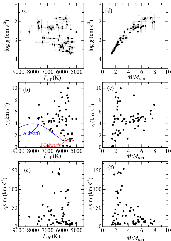
Figure 2: Graphical display of how $\log g$ (top panels), $v_{\rm t}$ (middle panels), and $v_{\rm e}\sin i$ (bottom panels) correlate with $T_{\rm eff}$ (left panels) or $M$ (right panels). In panel (b) are also depicted the mean $v_{\rm t}$ vs. $T_{\rm eff}$ relations for A dwarfs and F–G dwarfs by solid and dashed lines, respectively (see the caption of Fig. 10 in Paper I).

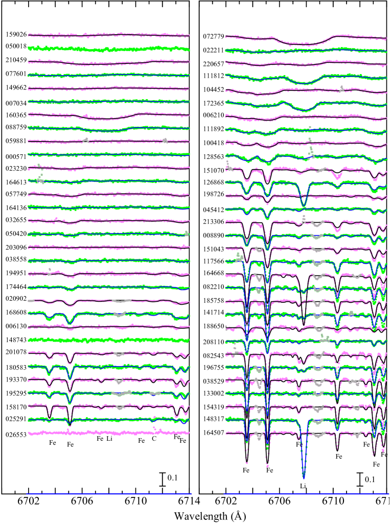
Figure 3: Synthetic spectrum fitting in the 6702–6714 Å region comprising the Li i 6708 line. Shown in the left and right panels are stars of $T_{\rm eff}>6000$ K and those for $T_{\rm eff}<6000$ K, respectively. The best-fit theoretical spectra are shown by solid lines. The observed data are plotted by symbols, where those used in the fitting are colored in pink or green, while those rejected in the fitting (e.g., unidentified lines or spectrum defect) are depicted in gray. In both panels, the spectra (indicated by the HD number) are arranged in the descending order of $v_{\rm e}\sin i$ with a vertical offset of 0.1 (in unit of the continuum level) applied to each spectrum relative to the adjacent one. Note that the fitting was impossible for HD 148753 and HD 026553, for which the spectra are almost featureless.

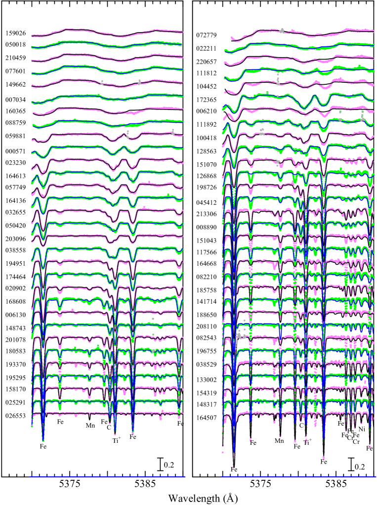
Figure 4: Synthetic spectrum fitting in the 5370–5390 Å region comprising the C i 5380 line. A vertical offset of 0.2 is applied to each spectrum relative to the adjacent one. Otherwise, the same as in Fig. 3.

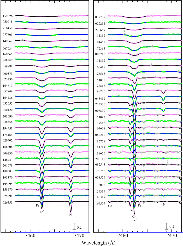
Figure 5: Synthetic spectrum fitting in the 7457–7472 Å region comprising the N i 7468 line. A vertical offset of 0.2 is applied to each spectrum relative to the adjacent one. Otherwise, the same as in Fig. 3.

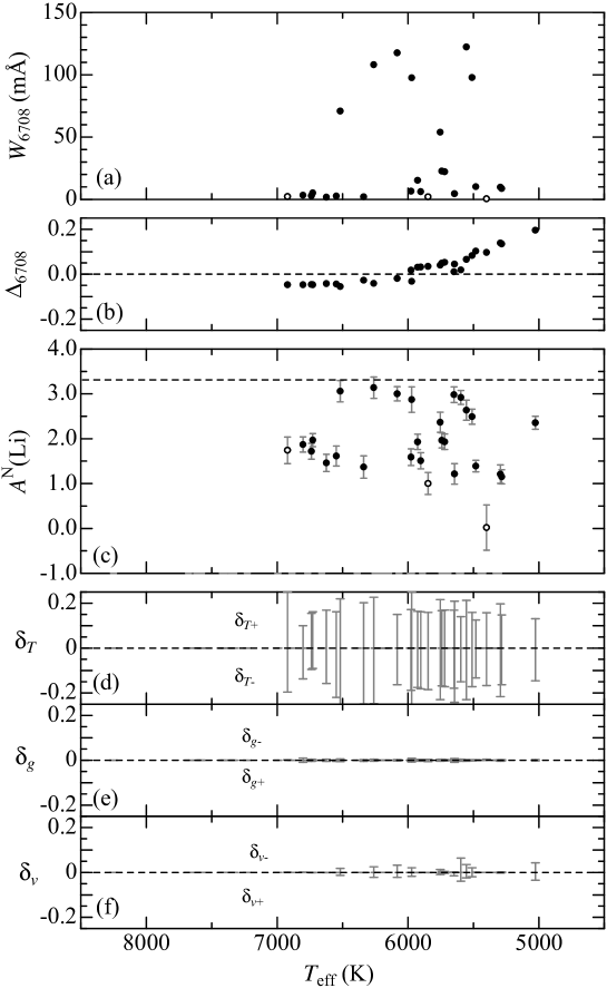
Figure 7: Lithium abundance and Li i 6708-related quantities plotted against $T_{\rm eff}$. (a) $W_{6708}$ (equivalent width of Li i 6708), (b) $\Delta_{6708}$ (non-LTE correction for Li i 6708), (c) $A^{\rm N}$(Li) (non-LTE abundance derived from Li i 6708) where the error bar denotes $\delta_{TgvW}$ (cf. Sect. 3.3), (d) $\delta_{T+}$ and $\delta_{T-}$ (abundance variations in response to the error in $T_{\rm eff}$), (e) $\delta_{g+}$ and $\delta_{g-}$ (abundance variations in response to the error in $\log g$), and (f) $\delta_{v+}$ and $\delta_{v-}$ (abundance variations in response to perturbing the $v_{\rm t}$ value by $\pm$max[$0.3v_{\rm t}$, 1 km s^-1]). The data shown in open circles in panels (a) and (c) denote unreliable results which were eventually discarded (cf. Sect. 3.3). The reference solar-system Li abundance of $A_{\rm ss}$ = 3.31 is indicated by the horizontal dashed line in panel (c).

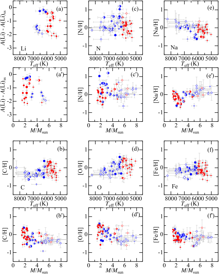
Figure 12: These six figure sets (a–f, each consisting of 2 panels) illustrate how the relative abundances of six elements (L, C, N, O, Na, and Fe) with respect to the reference abundances (the solar system abundance for Li; otherwise, the abundances of Procyon) depend upon $T_{\rm eff}$ (upper panel) or $M$ (lower panel). Different mass classes are discriminated by the symbol shape: filled circles $\cdots$ $M<2.5M_{\odot}$, half-filled circles $\cdots$ $2.5M_{\odot}<M<5M_{\odot}$, and open circles $\cdots$ $5M_{\odot}<M$. Different $v_{\rm e}\sin i$ classes are discriminated by the symbol size: small $\cdots$ $v_{\rm e}\sin i<10$ km s^-1, medium $\cdots$ 10 km s${}^{-1}<v_{\rm e}\sin i<50$ km s^-1, and large $\cdots$ 50 km s${}^{-1}<v_{\rm e}\sin i$. Stars of higher $T_{\rm eff}$ ($>6000$ K) and lower $T_{\rm eff}$ ($<6000$ K) are colored in blue and red, respectively. Regarding the meanings of the error bars, see Sect. 2 ($\sigma$ for $T_{\rm eff}$ as well as $M$) and Sect. 3.3 ($\delta_{TgvW}$ for the abundances).

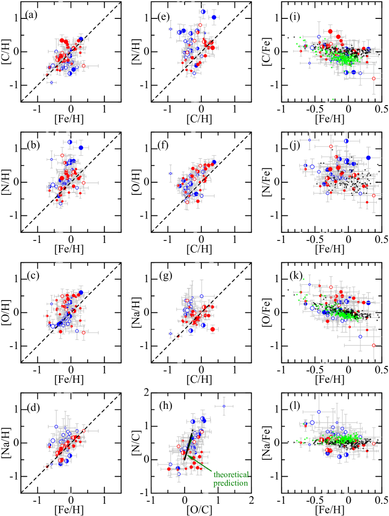
Figure 13: The left-hand and middle panels demonstrate the mutual correlations between the [C/H], [N/H], [O/H], [Na/H], and [Fe/H] values derived for our 62 program stars: (a) C vs. Fe, (b) N vs Fe, (c) O vs. Fe, (d) Na vs. Fe, (e) N vs. C, (f) O vs. C, and (g) Na vs. C. The relationship between [N/C] and [O/C] ratios is shown in panel (h), where the thick line is the theoretically predicted locus computed by Lagarde et al. (2012). [Although four different loci of solar metallicity models corresponding to the combination of (2 $M_{\odot}$, 6 $M_{\odot}$) and (standard mixing, non-standard mixing including thermohaline+rotational mixing) are overplotted here, they are hardly discernible from each other.] In the right-hand panels (i)–(l) are plotted the abundance ratios ([C/Fe], [N/Fe], [O/Fe], and [Na/Fe]) against [Fe/H], where the relations for 160 FGK dwarfs and 239 GK giants (cf. Fig. 10 in Takeda et al. 2015, while the [N/Fe] results for FGK dwarfs were taken from Takeda & Honda 2005) are also shown in black Greek crosses (+) and light-green St. Andrew’s crosses ($\times$), respectively. See the caption of Fig. 12 for the meanings of the other symbols. The error bars attached to the data points in panels (a)–(g) denote $\delta_{TgvW}$ described in Sect. 3.3, while the errors for [N/C] or [O/C] shown in panel (h) as well as those for [X/Fe] in panels (i)–(l) were evaluated as the root-sum-square of relevant two $\delta_{TgvW}$ values.

Figure 14: Comparison of the adopted stellar parameters and the resulting abundances in this study with those of Adamczak & Lambert (2014): (a) $T_{\rm eff}$, (b) $\log g$, (c) $v_{\rm t}$, (d) $v_{\rm e}\sin i$, (e) $M$, (f) [Fe/H], (g) [C/H], and (h) [O/H].

Appendix A On the source of abundance errors

Our analysis of 62 Hertzsprung-gap stars resulted in considerable scatters in the [C/H], [N/H], [O/H], [Na/H] and [Fe/H] abundances. The cause of such apparently large dispersions may deserve some examination. We here consider two possibilities: (i) errors in the atmospheric parameters and (ii) unusual atmospheric condition caused by stellar activity.

A.1 Uncertainties in atmospheric parameters

As one of the touchstones to judge the reasonability of our parameters adopted for each star ($T_{\rm eff}$ from reddening-corrected $B-V$ color, $\log g$ from parallax-based/extinction-corrected luminosity along with stellar mass estimated from evolutionary tracks; cf. Sect. 3 in Paper I), it is worthwhile to examine how they are compared with various published values determined in different ways. Although such a comparison was already tried by using the data taken from SIMBAD database in Paper I (see Fig. 2 therein), we here make use of the PASTEL database compiled by Soubiran et al. (2010) for the data source of $T_{\rm eff}$, $\log g$, and [Fe/H], the comparisons of which are shown in Fig. A1. The mean differences ($\pm\sigma$: standard deviation) are $\langle T_{\rm eff}\rangle$ (PASTEL$-$ours) = $26(\pm 380)$ K, $\langle\log g\rangle$ (PASTEL$-$ours) = $+0.01(\pm 0.45)$ dex, and $\langle$[Fe/H]$\rangle$ (PASTEL$-$ours) = $+0.15(\pm 0.18)$ dex. Meanwhile, regarding the errors we estimated for $T_{\rm eff}$, $\log g$, and [Fe/H] (cf. Sect. 2 for $T_{\rm eff}$ and $\log g$; Sect. 3.3 for [Fe/H]), their averages over all 62 stars are 280 K (ranging from 108 K to 788 K), 0.14 dex (ranging from 0.06 dex to 0.42 dex), and 0.19 dex (ranging from 0.06 dex to 0.44 dex), respectively. Comparing these with $\sigma$(PASTEL$-$ours) values mentioned above, we see that the discrepancy in $\log g$ is appreciably larger than our estimated uncertainties, which may reflects the intrinsic difficulty in determining the surface gravity for such high-luminosity stars. This situation is markedly different from the case of dwarf stars, where the spectroscopic $\log g$ and the luminosity-based $\log g$ based on the Hipparcos parallaxes (as adopted this study) agree with each other (see, e.g., Fig. 5 in Takeda et al. 2005). However, we do not consider that ambiguities in $\log g$ would lead to serious abundance errors, because of the insignificant gravity-sensitivity as can be seen in Fig. 7e–11e.

Besides, we compared our parameters ($T_{\rm eff}$, $\log g$, $v_{\rm t}$, and [Fe/H]) of comparatively sharp-lined G-type stars with the values spectroscopically determined by Takeda et al. (2005; 2 stars in common) and Takeda et al. (2008; 5 stars in common) based on the equivalent widths of Fe i and Fe ii lines, as displayed in Fig. A2. This figure indicates that, while a reasonable agreement is mostly confirmed for $T_{\rm eff}$, $\log g$, and [Fe/H], a distinct discrepancy is observed between our adopted $v_{\rm t}$ values of HD 82210 and HD 188650 (4.8 and 8.8 km s^-1, which were derived from O i lines in Paper I) and those determined by using Fe lines (1.1 and 2.2 km s^-1; cf. Fig. A2c). Since such large scale $v_{\rm t}$ values have occasionally been reported for evolved stars above the main sequence (see, e.g., the references quoted in Sect. 4.2 of Gray 1978), we would reserve the decision of which is correct. Yet, we should keep in mind a possibility that the prominently large $v_{\rm t}$ values up to $\lesssim 10$ km s^-1 around $T_{\rm eff}\sim 6000$ K (cf. Fig. 2b) may be spurious (i.e., erroneous overestimation), even though these are the unique solutions which could satisfy the non-LTE abundance consistency between the O i 7771–5 and O i 6156–8 features. For example, such an overestimation of $v_{\rm t}$ from O i lines may happen when the stronger O i 7771–5 triplet suffers an extra intensification by a chromospheric temperature rise in the upper atmosphere (cf. Takeda 1995b). (Interestingly, both of these HD 82210 and HD 188650 show core emissions in the core of the Ca ii K line; cf. Fig. A3). In any event, since the resulting abundances are insensitive to a change in $v_{\rm t}$ (because the relevant lines are fairly weak and the thermal velocity is large for these light elements; cf. Fig. 7f–11f), it is unlikely that ambiguities in $v_{\rm t}$ can cause significant abundance errors in the present case.

Considering what has been described above and that the most important parameter affecting the abundance is $T_{\rm eff}$ (cf. Fig. 7d–11d), we feel that our error bars shown in Fig. 12 and Fig. 13 (which are determined mainly by ambiguities in $T_{\rm eff}$ typically by $\sim 300$ K on the average) are not seriously misvalued in the general sense, although some cases of considerably wrong abundances caused by exceptionally large parameter errors can not be excluded.

A.2 Possibility of influential chromospheric activity

In connection with the large scatter observed in our abundances (e.g., [X/Fe] vs. [Fe/H] diagrams shown in Fig. 13i–l), it is worth noting that Takeda & Tajitsu (2017) similarly reported anomalously large dispersion in the C and O abundances (derived from C i 5380 and O i 7771–5 lines of high excitation) in a fraction of Li-rich G-type giants (cf. Figs. 14a and 14c therein), which they considered nothing but a superficial phenomenon caused by high chromospheric activity. Regarding such activity-related effects, two mechanisms may be possible. The first is the temperature rise in the upper layer, by which high-excitation lines of dominant-stage species (such as C i, N i, or O i) can be strengthened (see Sect. 9 in Takeda & Tajitsu 2017). The second is the enhanced UV radiation, by which the lines of minor-population species (such as Fe i or Na i) are weakened due to the overionization effect. The apparent underabundances of heavier elements (such as Fe) in the secondary component of Capella (G0 iii giant of high activity) compared to the primary (normal G8 iii giant) concluded by Takeda et al. (2018b) can be attributed to this mechanism (cf. Sect. 6.3 therein).

Meanwhile, as to the abundances obtained in this study, we see from Fig. 12 that (1) apparently deviated data points are prominently large [C/H], [N/H], and [O/H] (even up to $\sim+1$) and unusually small [Na/H] (down to $\sim-0.7$), (2) the large abundance dispersion tends to be seen in lower $T_{\rm eff}$ ($<6500$ K) stars cooler than the granulation boundary (see, e.g., Gray 2005), and (3) stars showing large deviation tend to have comparatively large $v_{\rm e}\sin i$. Therefore, it may be a ponderable interpretation that high chromospheric activity caused by rapid rotation in cooler stars having deep convection zone (in which rotation-induced dynamo mechanism can operate) would have especially intensified the C i 5380, N i 7460, and O i 6156–8 lines (all high-excitation lines of dominant species) and weakened the Na i 6161 line (minor population species).

Motivated by this idea, we checked the Ca ii K line at 3933.663 Å for each star in order to search for any core emission indicative of strong chromospheric activity, making use of the fact that our spectral data cover wide wavelength range down to the violet region. The spectra in the 3920–3950 Å portion are displayed in Fig. A3 for all 62 stars. Although the S/N ratios at the core of this strong line are insufficient in not a few cases (because of the decreased detector sensitivity in this short wavelength region along with the considerably low flux level), which makes examination of weak feature difficult, the following characteristics can be read from this figure.

• Clear core emission is hardly seen for stars of higher $T_{\rm eff}$ ($>6000$ K) (cf. the left panel of Fig A3), though only a weak sign is observed for a few stars such as HD 158170 (8.4), 193370 (9.3), 180583 (9,9) which are between 6000 K $\lesssim T_{\rm eff}\lesssim 6500$ K (given in the parentheses are the corresponding $v_{\rm e}\sin i$ values).

• Regarding lower $T_{\rm eff}$ ($<6000$ K) stars expected have deep convective envelopes, emission components are observed in about $\sim 1/3$ of them (cf. the right panel of Fig A3) such as HD 133002 (6.6), 188650 (7.7), 141714 (7.7), 185758 (8.4), 82210 (8.6), 164668 (9.5), 117566 (11.1), 45412 (13.1), 198726 (14.7), 126868 (16.5), and 111812 (64.6).

• In summary, regarding our sample stars, emission feature in the Ca ii K line is observed in a significant fraction of $T_{\rm eff}<6500$ K stars, though really strong emission is seen only a few among them. Interestingly, however, such a feature tends to be detected mostly in not-so-rapid rotators of $v_{\rm e}\sin i$ around $\sim 10$ km s^-1, while not in rapid rotators except for HD 111812.

Therefore, our speculation that rapidly rotating stars would have higher activity could not be confirmed (though this does not mean that rapid rotators have no chromospheric activity because weak feature may possibly be smeared out for such broad-line cases). We also examined whether any connection exists between the abundance anomaly and the Ca ii core emission. For example, regarding the five stars showing anomalous [O/Fe] ratio larger than +0.5 (cf. Fig. 13k) [HD 45412 (+0.76), 164668 (+0.80), 82210 (+0.52), 100418 (+0.62), 208110 (+0.61)], although the former three surely show emission features (especially that of HD 82210 is strong), such a detection is difficult (i.e., buried in noises) for the latter two, which means that a clear relationship can hardly be concluded. Accordingly, as far as this examination of Ca ii K line profile is concerned, we could not find any convincing evidence in support of the interpretation that large abundance scatter may have stemmed from unusual atmospheric condition caused by stellar chromospheric activity. It thus seems premature to ascribe the reason for the large abundance dispersion to this hypothesis.

Figure 1: Comparison of the stellar parameters adopted in this study (taken from Paper I) with those from various publications compiled in the PASTEL database (Soubiran et al. 2010): (a) $T_{\rm eff}$ (175 data for 57 stars in common), (b) $\log g$ (99 data for 40 stars in common), and (c) [Fe/H] (106 data for 42 stars in common).

References

- [Adamczak(2014)] Adamczak, J., & Lambert, D. L. 2014, ApJ, 791, 58.
- [Anthony(2018)] Anthony-Twarog, B. J., Lee-Brown, D. B., Deliyannis, C. P., & Twarog, B. A. 2018, AJ, 155, 138.
- [Barbuy(1996)] Barbuy, B., De Medeiros, J. R., & Maeder, A. 1996, A&A, 305, 911.
- [deLaverny(2003)] de Laverny, P., do Nascimento Jr., J. D., Lèbre, A., De Medeiros, J. R. 2003, A&A, 410, 937.
- [Gray(1978)] Gray, D. F. 1978, Solar Phys., 59, 193.
- [Gray(2005)] Gray, D. F. 2005, The Observation and Analysis of Stellar Photospheres, 3rd ed. (Cambridge: Cambridge University Press).
- [Kurucz(1993)] Kurucz, R. L. 1993, Kurucz CD-ROM, No. 13 (Harvard-Smithsonian Center for Astrophysics).
- [Kurucz(1995)] Kurucz, R. L., & Bell, B. 1995, Kurucz CD-ROM, No. 23, (Harvard-Smithsonian Center for Astrophysics).
- [Lagarde(2012)] Lagarde, N., Decressin, T., Charbonnel, C., Eggenberger, P., Ekström, S., & Palacios, A. 2012, A&A, 543, A108.
- [Lejeune(2001)] Lejeune, T., & Schaerer, D. 2001, A&A, 366, 538.
- [Luck(1985)] Luck, R. E., & Lambert, D. L. 1985, ApJ, 298, 782.
- [Lyubimkov(2011)] Lyubimkov, L. S., Lambert, D. L., Korotin, S. A., Poklad, D. B., Rachkovskaya, T. M., & Rostopchin, S. I. 2011, MNRAS, 410, 1774.
- [Lyubimkov(2004)] Lyubimkov, L. S., Rostopchin, S. I., & Lambert, D. L. 2004, MNRAS, 351, 745.
- [Molina(2016)] Molina, R. E., & Rivera, H. 2016, RMxAA, 52, 399.
- [Smiljanic(2006)] Smiljanic, R., Barbuy, B., De Medeiros, J. R., & Maeder, A. 2006, A&A, 449, 655.
- [Smiljanic(2018)] Smiljanic, R., Donati, P., Bragaglia, A., Lemasle, B., &, Romano, D. 2018, A&A, 616, A112.
- [Smith(1998)] Smith, V. V., Lambert, D. L., & Nissen, P. E. 1998, ApJ, 506, 405.
- [Soubiran(2010)] Soubiran, C., Le Campion, J.-F., Cayrel de Strobel, G., & Caillo, A. 2010, A&A, 515, 111.
- [Takeda(1995a)] Takeda, Y. 1995a, PASJ, 47, 287.
- [Takeda(1995b)] Takeda, Y. 1995b, PASJ, 47, 463.
- [Takeda(2018b)] Takeda, Y., Hashimoto, O., & Honda, S. 2018b, ApJ, 862, 57.
- [TakedaHonda(2005)] Takeda, Y., & Honda, S. 2005, PASJ, 57, 65.
- [Takeda(2018a)] Takeda, Y., Jeong, G., & Han, I. 2018a, PASJ, 70, 8. (Paper I)
- [Takeda(2013)] Takeda, Y., Kang, D.-I., Han, I., Lee, B.-C., & Kim, K.-M. 2013, MNRAS, 432, 769.
- [Takeda(2018c)] Takeda, Y., Kawanomoto, S., Ohishi, N., Kang, D.-I., Han, I., Lee, B.-C., & Kim, K.-M. 2018c, PASJ, 70, 91. (Paper II)
- [Takeda(2005)] Takeda, Y., Ohkubo, M., Sato, B., Kambe, E., & Sadakane, K. 2005, PASJ, 57, 27.
- [Takeda(2008)] Takeda, Y., Sato, B., & Murata, D. 2008, PASJ, 60, 781.
- [Takeda(2015)] Takeda, Y., Sato, B., Omiya, M., & Harakawa, H. 2015, PASJ, 67, 24.
- [Takeda(1994)] Takeda, Y., & Takada-Hidai, M. 1994, PASJ, 46, 395.
- [Takeda(2017)] Takeda, Y., & Tajitsu, A. 2017, PASJ, 69, 74.
- [vanLeeuwen(2007)] van Leeuwen, F. 2007, Hipparcos, the New Reduction of the Raw Data (Berlin: Springer)