Critical hysteresis on dilute triangular lattice

Abstract

Critical hysteresis in the zero-temperature random-field Ising model on a two-dimensional triangular lattice has been studied earlier with site dilution on one sublattice. It was reported that criticality vanishes if less than one third of the sublattice is occupied. This appears at variance with recently obtained exact solutions of the model on dilute Bethe lattices and prompts us to revisit the problem using an alternate numerical method. Contrary to our speculation that criticality may not be exactly zero below one third dilution, the present study indicates it is nearly zero if approximately less than two-thirds of the sublattice is occupied. This suggests that hysteresis on dilute periodic lattices is qualitatively different from that on dilute Bethe lattices. Possible reasons are discussed briefly.

I Introduction

The random-field Ising model imryma was introduced to study the effect of quenched disorder on a system’s ability to sustain long-range order in thermal equilibrium. After a rather prolonged debate it was resolved that the lower critical dimension of the Ising model ising remains equal to two in the presence of quenched random fields imbrie . Subsequently a zero-temperature version of the model (ZTRFIM) without thermal fluctuations but an on-site quenched random field distribution N[0,$\sigma^{2}$] was introduced  sethna1 ; sethna2 as a model for disorder-driven hysteresis in ferromagnets and other similar systems sethna3 . Numerical simulations of ZTRFIM on a simple cubic lattice reveals a critical value of $\sigma=\sigma_{c}\approx 2.16J$ ($J$ being the nearest neighbor ferromagnetic exchange interaction). For $\sigma<\sigma_{c}$ each half of the hysteresis loop shows a discontinuity in magnetization. The size of the discontinuity decreases to zero at a critical value of the applied field $h_{c}\approx 1.435J$ as $\sigma$ is increased to $\sigma_{c}$. The behavior near $\{h_{c},\sigma_{c}\}$ shows scaling and universality quite similar to the one caused by critical thermal fluctuations at an equilibrium critical point. These aspects of the model are important in understanding hysteresis experiments and related theoretical issues. Initial numerical attempts to find a $\sigma_{c}$ on the square lattice were inconclusive casting doubt on the lower critical dimension of the model. More extensive simulations  spasojevic indicate $\sigma_{c}\approx 0.54J$ and $h_{c}\approx 1.275J$ on the $2d$ square lattice.

An exact solution dhar of ZTRFIM on a Bethe lattice of integer connectivity $z$ shows that criticality occurs only if $z\geq 4$. Normally critical behavior on Bethe lattices is independent of $z$ if $z>2$ and is the same as in the mean field theory. Therefore the result for hysteresis is unusual and efforts have been made  handford to understand the physics behind it. A useful insight is obtained by extending the analysis to noninteger values of $z$  shukla1 ; shukla2 . This is done by considering lattices where the connectivity of each node is distributed over a set of integers so that the average connectivity of a node has a noninteger value greater than two. Fortunately the problem can still be solved exactly and leads to the identification of a general criterion for the occurrence of critical hysteresis. The general criterion is that there should be a spanning path across the lattice and a fraction of sites on this path (even an arbitrarily small fraction) should have connectivity $z\geq 4$.

On periodic lattices, an exact solution of ZTRFIM is not available. Extant simulations indicate that the existence or absence of $\sigma_{c}$ on a periodic lattice with uniform connectivity $z$ is the same as on a Bethe lattice of connectivity $z$. Criticality is absent on any lattice with $z=3$ irrespective of the dimension $d$ of the space in which the lattice is embedded  sabhapandit . Indeed critical hysteresis appears to be determined by a lower integer connectivity $z_{\ell}=4$ rather than a lower critical dimension $d_{\ell}=2$. As $z$ increases above $z_{\ell}$, the critical point becomes easier to observe in simulations. Compared with the intensive simulations on large square lattices, it takes a modest effort to observe criticality on a triangular lattice  diana . However the estimated value of $\sigma_{c}$ appears to decrease slowly with increasing size of lattice. A study on lattices of size $L\times L$ with $L\leq 600$ gives $\sigma_{c}=1.22$  kurbah , while more extensive simulations on lattices of size up to $L\leq 65536$ yield $\sigma_{c}=0.85$  janicevic . We may remark that the critical exponents on the triangular lattice appear to be different from those on the square lattice  janicevic . This is puzzling in the context of the universality of critical phenomena and the broader implications of this result are not clear. At present $L=65536$ is the largest linear size that has been studied thoroughly using available computers. One may ask if $\sigma_{c}$ would decrease further in case much larger values of $L$ were studied. Although extant numerical studies do not suggest $\sigma_{c}\to 0$ as $L\to\infty$ but we are not aware of a rigorous argument for the same. Questions of this nature can not be resolved conclusively by numerical studies. Criticality on a dilute lattice is even harder to settle numerically due to additional positional disorder. Keeping this in mind, our focus in the present paper is on systems of modest sizes and try to understand the qualitative trends in the basic data.

It has been argued that $\sigma_{c}=0$ for an asymmetric distribution of the random field in case $z=3$ and $\sigma_{c}>0$ for integer values $z\geq 4$  sabhapandit . Our object here is to examine non-integer values of $z>3$. A dilute (partially occupied) lattice of connectivity $z$ enables us to study a lattice of average connectivity $z_{av}<z$. We consider a triangular lattice $T=A+B+C$ with one of its constituent sublattices, say $C$, having a reduced occupation probability $c$  kurbah . The average connectivity on $T$ is then equal to $z_{av}=6(1+2c)/(2+c)$ and the average connectivity on $A$ or $B$ sublattice is equal to $z_{eff}=3(1+c)$. The connectivity of occupied sites on $C$ is equal to six. As $c$ is reduced from $1$ to $0$, we go from a triangular to a honeycomb lattice. Extant work indicates that $\sigma_{c}$ drops to zero at $c=1/3$ within numerical errors. At $c=1/3$, $z_{eff}=4$. Keeping in mind that $z\geq 4$ is required for criticality on lattices of uniform integer connectivity $z$, it does look reasonable at first sight that $\sigma_{c}=0$ for $c<1/3$ on a diluted lattice. However recent studies  shukla1 ; shukla2 on Bethe lattices of mixed coordination number bring out a new twist in the importance of sites with connectivity $z\geq 4$. Criticality has been shown to exist even if a fraction of occupied sites have $z<4$ but there should be a spanning path through occupied sites and a fraction of sites on this path should have $z\geq 4$. If this criterion were to apply to dilute periodic lattices as well, we may expect a non-zero $\sigma_{c}$ in the entire range $1\geq c>0$.

The reason for a discontinuity in the hysteresis loop on a Bethe lattice is that a fixed point corresponding to zero magnetization becomes unstable and splits into two stable fixed points for $\sigma<\sigma_{c}$. The size of the splitting is the size of the discontinuity. This is easily demonstrated by an analysis of the model on a Cayley tree  shukla2 . We set the applied field equal to zero, and consider an initial configuration with all spins down except the spins on the surface of the tree. If the surface spins are equally likely to be up or down i.e. if the surface magnetization is zero it remains zero as spins are relaxed layer by layer towards the interior of the tree. Small perturbations to the surface magnetization behave differently depending on the connectivity $z$ of the lattice. If $z\leq 3$ the perturbations decrease and the magnetization in the deep interior remains zero. If $z\geq 4$, the perturbations diverge. A positive value of magnetization tends to increase, and and a negative value tends to decrease as we move towards the interior. An important point is that this is not just a global property of a lattice of uniform connectivity $z$. On a lattice with mixed connectivity, each node depending on its connectivity $z$ increases or decreases the perturbation passing through it in a similar fashion. Larger the connectivity of the node, larger is the enhancement. Thus a small perturbation on the surface leads to a finite discontinuity in the deep interior of the tree if a fraction of nodes along the path have $z\geq 4$. Of course a spanning path is a prerequisite to reach the deep interior. However spanning paths are always there under our scheme of dilution. Even if $c=0$, there are spanning paths on the honeycomb lattice; $c>0$ introduces additional paths containing $C$ sites. The $C$ sites have connectivity equal to six. As long as there are some $C$ sites there are spanning paths punctuated by sites with connectivity equal to six. Remaining sites, the $A$ and $B$ sites have connectivity $3(1+c)$ on the average. If $c\geq 1/3$ the average connectivity of each site on the spanning path is greater than four and we have a case for a relatively large discontinuity as observed in extant simulations. On the other hand, if $c<1/3$, we should still expect a discontinuity albeit a much smaller one. The argument in favor of it is the enhancement effect of nodes with $z\geq 4$ on a Bethe lattice. It is not clear a priori how loops on a periodic lattice may vacate this effect. This forms the motivation to review critical hysteresis on the dilute triangular lattice. However simulations presented below suggest that criticality on a dilute triangular lattice is qualitatively different from that on a dilute Bethe lattice.

It may not be out of place to make two general remarks on hysteresis studies in ZTRFIM before getting into the specifics of the present paper. Firstly, setting temperature and driving frequency equal to zero is an approximation. Hysteresis in physical systems is necessarily a finite temperature and finite time phenomena. A key feature of ZTRFIM is the occurrence of a fixed point under the zero-temperature dynamics. Scale invariance around the fixed point is directly related to experimental aspects of Barkhausen noise. The fixed point at $\sigma_{c}$ is lost if any of the two approximations are relaxed  shukla3 . This is disconcerting but does not end the usefulness of ZTRFIM. The model has been applied to a variety of social phenomena including opinion dynamics where the zero temperature Glauber dynamics is not so unrealistic  shukla4 . Therefore efforts to improve our technical understanding of ZTRFIM on different lattices and their associated universality classes would remain of value in statistical mechanics.

II The Model and Numerical Results

In order to make the paper self-contained and better readable, we describe the model briefly. Readers may refer to  kurbah for more details. The Hamiltonian is,

$$H=-J\sum_{i,j}s_{i}s_{j}-\sum_{i}h_{i}s_{i}-h\sum_{i}s_{i}.$$ (1)

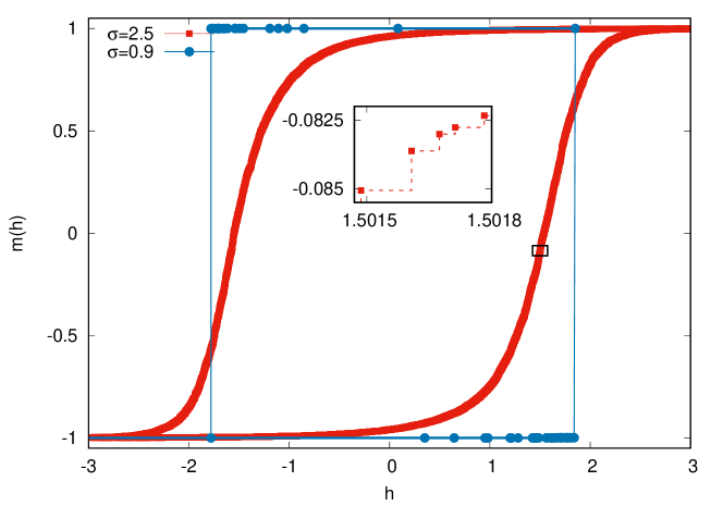
Figure 1: Hysteresis loops in the zero-temperature random-field Ising model for N(0,$\sigma^{2}$) distribution of the random-field on an $L\times L$ triangular lattice with $L=333$ and $\sigma_{c}(L)\approx 1.2$. Loops are discontinuous for $\sigma<\sigma_{c}(L)$ but macroscopically smooth for $\sigma\geq\sigma_{c}(L)$. At microscopic level they exhibit Barkhausen noise as shown in the inset.

J is ferromagnetic interaction, the double sum is over nearest neighbors of a 2d triangular lattice of size $N=L\times L$; $s_{i}=\pm 1,i=1,\ldots,N$ are Ising spins; $h_{i}$ is a quenched random field drawn from a distribution N(0,$\sigma^{2}$) and $h$ is an external field that is ramped up adiabatically from $-\infty$ to $\infty$ and back down to $-\infty$. The triangular lattice comprises three sublattices $A$, $B$, and $C$; $A$ and $B$ are fully occupied but sites on $C$ sublattice are occupied with probability $c$ $(0\leq c\leq 1)$. Thus we have a triangular lattice at $c=1$, but a honeycomb lattice at $c=0$. Hysteresis under zero-temperature Glauber dynamics is studied as follows. Depending upon the size of the system N, we start with a sufficiently large and negative $h=-h_{0}$ such that the state $\{s_{i}=-1\}$ is stable. A stable configuration has each spin $s_{i}$ aligned along the local field $\ell_{i}=nJ-(z-n)J+h_{i}+h$ at its site; here $z$ is the number of nearest occupied neighbors of $i$; $n$ neighbors being up ($s=1$), and $(z-n)$ down ($s=-1$). The magnetization per spin in a stable state is $m(h)=N^{-1}\sum_{i}s_{i}$. Thus we start with a stable state with $m(-h_{0})=-1$. Now we increase $h$ by the minimal amount, say $h=h_{1}=-h_{0}+\delta h_{1}$ that makes one of the spins unstable. An attempt to stabilize this spin may make some or all of its neighbors unstable. We hold $h=h_{1}$ constant and iteratively flip up unstable spins until no spins in the system are unstable. This results in an avalanche of flipped spins in the vicinity of the initial unstable spin. The increase of magnetization from $h=h_{0}$ to $h=h_{1}$ is equal to twice the size of the avalanche. Holding the applied field constant during the avalanche corresponds to the assumption that the applied field varies infinitely slowly in comparison with the spin relaxation rate. The stable state at the end of an avalanche corresponds to a local minimum in the energy landscape, and depends on the history of the system. In our example the local minimum retains memory of the initial state with $m(-h_{0})=-1$. Under finite temperature Glauber dynamics, the system may escape the local minimum and move towards the global minimum albeit very slowly. For this reason we may occasionally refer to the stable state under zero temperature dynamics as a metastable state. Employing the above procedure repeatedly, we determine all the metastable states between $m(-h_{0})=-1$ and $m(h_{0})=1$ on lower half of the hysteresis loop, and similarly on the upper half as well. Fig.1 depicts the result for $c=0.90$ and $\sigma=0.9$ and $\sigma=2.5$ respectively. The key point is that for smaller $\sigma$ the loop has discontinuities while there is no discontinuity for larger $\sigma$. The upper and lower halves of the loop are related by symmetry and therefore it suffices to focus only on the lower half. Apparently, there is a critical value $\sigma=\sigma_{c}$ which separates discontinuity at $\sigma<\sigma_{c}$ from no discontinuity at $\sigma>\sigma_{c}$ but the numerical determination of $\sigma_{c}$ is a challenging task.

Our main interest is to understand the qualitative dependence of $\sigma_{c}$ on $L$ and $c$, and to check in particular if $\sigma_{c}$ drops to zero abruptly when $c$ drops below $c=1/3$. The defining feature of $\sigma_{c}$ is that the discontinuity in the magnetization $m(h)$, say on the lower half of the hysteresis loop, reduces to zero as $h\to h_{c}$ and $\sigma\to\sigma_{c}$ from below. Exact solution on Bethe lattice and simulations on periodic lattices reveal that a discontinuity in magnetization is accompanied by a reversal of magnetization. Numerical determination of a discontinuity is rather problematic. For small $\sigma$, the graph $m(h)$ vs. $h$ near $m(h)=0$ tends to be almost vertical anyway. A simulation based on a single realization of the random-field distribution necessarily shows a broken curve comprising a few irregularly placed discontinuities due to large fluctuations in the system. The number as well as positions of discontinuities vary from configuration to configuration and averaging over configurations results in a steep but smooth $m(h)$ curve. A genuine underlying discontinuity, if any, has to be inferred from the character of fluctuations. An added complication is that fluctuations at a discontinuity are different from those at the critical point where the discontinuity vanishes. Finally finite size scaling has to be employed to infer $\sigma_{c}$ in the thermodynamic limit. The estimate for $\sigma_{c}$ using finite size scaling should be independent of system sizes used in numerical simulations. However numerical uncertainties are large and diminish extremely slowly with increasing system size. As mentioned earlier, initial studies on triangular lattices of sizes $L\times L$ with $L\leq 600$ indicated $\sigma_{c}=1.22$  kurbah but more extensive simulations on lattices up to $L=65536$ yield $\sigma_{c}=0.85$  janicevic . The procedure for determining $\sigma_{c}$ is rather indirect, tedious, cpu intensive, and various compromises have to be made in order to draw reasonable conclusions kurbah .

In this paper we adopt a different approach than used in previous studies. The basic idea is simple although the details have similar issues as in earlier studies. The new approach is useful in discerning important trends in the behavior of the model based on simulations of systems of modest sizes. For a fixed $\sigma$ on an $L\times L$ lattice, we count the total number of metastable states $M(\sigma;L)$ (fixed points under zero temperature Glauber dynamics) comprising the lower half of hysteresis loop. As indicated in the previous paragraph we increase the applied field $h$ by a minimal amount to go from one fixed point to the next and keep $h$ fixed during the relaxation process. We plot $M(\sigma;L)$ as a function of $\sigma$. It is a monotonically increasing function of $\sigma$ without any discontinuity. The cpu time increases rapidly with increasing $L$ and $\sigma$. Fig.2 shows the result on a modest $33\times 33$ triangular lattice and $0<\sigma\leq 50$. The general features of Fig.2 are easy to understand. In the limit of small $\sigma$, $\sigma\leq 0.4$ approximately, the first spin to flip up initiates an infinite avalanche of flipped spins giving $M(\sigma<0.4;L)=2$. In the limit $\sigma\to\infty$, spins flip up independently and $M(\sigma\to\infty;L)$ increases towards $L\times L$. We expect $M(\sigma;L)$ to increase continuously from $2$ to $L\times L$ as $\sigma$ increases from $0$ to $\infty$ on a finite lattice. This expectation is born out by Fig.2. If there is a critical value of $\sigma$ separating discontinuous $m(h)$ for $\sigma<\sigma_{c}(L)$ with continuous $m(h)$ for $\sigma>\sigma_{c}(L)$ we ought to see its signature in the $M(\sigma;L)$ graph. A discontinuity in $m(h)$ for $\sigma<\sigma_{c}$ would effectively reduce $M(\sigma;L)$ in proportion to its size. This would result in some change in shape of $M(\sigma;L)$ $vs.$ $\sigma$ graph at $\sigma_{c}(L)$. We find that this effect is present but too weak to be seen with naked eye in the main graph of Fig.2 or its magnified portion in the range $0<\sigma<4$ shown in the left inset there. However, we do see an apparent inflexion point around $\sigma\approx 1.8$ if $M(\sigma;L)$ is plotted on logscale scale as in the right inset.We tentatively identify this inflexion point with $\sigma_{c}(L)$, the critical $\sigma_{c}$ on an $L\times L$ lattice. A scaling property of $M(\sigma;L)$ with respect to $L$ presented below confirms this identification.

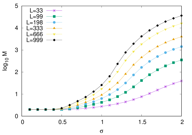
Figure 3: $\log_{10}M$ $vs.$ $\sigma$ in the range $0<\sigma<2$ on an $L\times L$ triangular lattice; $L=33,99,198,333,666$, and $999$. M is averaged over $10^{4}$ configurations for $L\leq 198$ and $10^{3}$ configurations for $L>198$. As $L$ increases, the inflexion point $\sigma_{c}(L)$ in the corresponding graph shifts to lower $\sigma$.

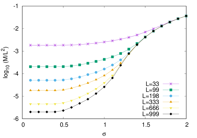
Figure 4: The data in Fig.2 for the triangular lattice is replotted to show $\log_{10}\frac{M}{L^{2}}$ vs. $\sigma$. $M\to 2$ as $\sigma\to 0$ irrespective of $L$. It is therefore an artifact of scaling that graphs fan out for smaller values of $\sigma$. The interesting feature is that they overlap for larger values of $\sigma$. This feature may be exploited to estimate $\sigma_{c}$.

Fig.3 shows $\log_{10}M(\sigma;L)$ $vs.$ $\sigma$ on a triangular lattice for $0<\sigma<2$ and $L=33,99,198,333,666,999$. The results have been averaged over $10^{4}$ configurations of the random field distribution for $L\leq 198$ and $10^{3}$ configurations for $L\geq 333$. As expected, the graphs start at $\log_{10}2$ and fan out towards $\log_{10}L$ with increasing $\sigma$. There is an apparent scaling with respect to $L$. Fig.4 brings out this scaling explicitly by plotting $G(\sigma;L)$ where $G(\sigma;L)=\log_{10}{\frac{M(\sigma)}{L\times L}}$. The quantity $G(\sigma;L)$ is the logarithm of the density of metastable states per unit area of the lattice. Each $G(\sigma;L)$ has an apparent inflexion point at $\sigma_{c}(L)$ being concave up for $\sigma<\sigma_{c}(L)$, and convex up $\sigma>\sigma_{c}(L)$. Graphs for $\sigma>\sigma_{c}(L)$ merge into each other from above meaning they maintain their relative order in $L$ as they merge. It is easy to understand this behavior. Each metastable state is associated with an avalanche that precedes it. Therefore we may visualize a metastable state as an area on the $L\times L$ lattice occupied by spins that turn up together in an avalanche. It helps to understand the following discussion if we imagine coloring the area occupied by each avalanche with a different color. $G(\sigma,L)$ is then the logarithm of the density of colors when colors fill the entire lattice. Inverse of the density gives the average area occupied by a randomly chosen color. Independence of $G(\sigma;L)$ from $L$ for $\sigma>\sigma_{c}(L)$ suggests that colors are well dispersed and each color is spread over a much smaller area than $L\times L$. In other words, it suggests the absence of a large spanning avalanche of the order of $L\times L$. The curve is convex up because $G(\sigma;L)$ increases with increasing $\sigma$ and approaches saturation in the limit $\sigma\to\infty$. In contrast, $G(\sigma;L)$ for $\sigma<\sigma_{c}(L)$ depends on $L$ and is concave up. This too is understandable. In this regime, there is a spanning cluster on the scale $L\times L$. Let us color it black. The black cluster contributes merely one color to the lattice but takes up a disproportionately huge area preventing more colors from getting in. This significantly reduces $G(\sigma;L)$. The black cluster shrinks to zero as $\sigma\to\sigma_{c}(L)$ from below. The area vacated by the shrinking cluster is gradually filled up by smaller clusters of different colors thus increasing $G(\sigma;L)$. This explains the concave up shape as well as the $L$-dependence of $G(\sigma;L)$ for $\sigma<\sigma_{c}(L)$. These considerations lead us to associate the inflexion point on $G(\sigma;L)$ curve with $\sigma_{c}(L)$. In the following, we examine how $\sigma_{c}(L)$ shifts to lower values with increasing $L$. However, before describing the numerical work, we may draw attention to a practical limitation of our analysis.

We evaluate $G(\sigma)$ on six lattices of size $33\leq L\leq 999$ for $0.1J\leq\sigma\leq 2.0J$. The range of $\sigma$ is chosen because $\sigma_{c}(L)\approx 1.8J$ for $L=33$ and it is expected to decrease for larger $L$. We increment $\sigma$ in steps of $\delta\sigma=0.1$, getting $20$ data points for each $L$. Fitting the 20 points to a polynomial of degree 10 or so results in a reasonably good looking fit but the fitted curve has a wavy nature on a magnified scale. Taking the second derivative of the curve to find the inflexion point $\sigma_{c}(L)$ introduces errors and creates spurious inflexion points as well. To avoid the spurious inflexion points we adopt an alternate method which does not require fitting the data to a polynomial and serves to double check our results. We take $\sigma_{c}(L)$ as the point where $G(\sigma;L)$ vs $\sigma$ curve merges with the corresponding curve for the next higher value of $L$. In other words we take $G(\sigma;L)$ curve for $L=999$ as the boundary and $\sigma_{c}(L)$ for $L<999$ as the point where the corresponding curve merges with the boundary. This procedure necessarily introduces an error due to the fixed increment $\delta\sigma$. In the absence of interpolations between values of $\sigma$ at fixed intervals, $\sigma_{c}(L)$ is restricted to one of the input values. However it produces qualitatively similar result as obtained by fitting the data to polynomials. We will return to this point when discussing our results in the following.

Let us call L33 the graph in Fig.4 corresponding to L=33 and similarly L99 etc. We find that L33 merges with L99 for $\sigma\geq 1.8$; L99 merges with L198 for $\sigma\geq 1.5$; L198 merges with L333 for $\sigma\geq 1.4$; L333 merges with L666 for $\sigma\geq 1.3$; L666 merges with L999 for $\sigma\geq 1.2$. As discussed in the preceding paragraph, we interpret these results as indicating $\sigma_{c}(L)=1.8,1.5,1.4,1.3,1.2$ for systems of linear size $L=33,99,198,333,666$ respectively. If we fit $\sigma_{c}(L)$ to a power law scaling of the form

$$\sigma_{c}(L)=\sigma_{c}+a\times L^{-b}$$ (2)

we find $\sigma_{c}(L)$ converges to $\sigma_{c}=0.81\pm 0.19$ in the limit $L\to\infty$ with $a=2.85\pm 0.37$ and $b=0.30\pm 0.09$. We have also fit $G(\sigma)$ $vs.$ $\sigma$ data to polynomials of degree eleven, and looked for inflexion points on the resulting continuous curve. Ignoring the spurious inflexion points near the boundaries of the range $[0.1\leq\sigma\leq 2.0]$, we obtain $\sigma_{c}(L)=1.68,1.48,1.38,1.32,1.25,1.20$ for $L=33,99,198,333,666,999$ respectively. Fitting these values to Eq.2 yields $\sigma_{c}=0.84\pm 0.06$, $a=1.97\pm 0.05$, and $b=0.24\pm 0.03$. It is satisfying that the values of $\sigma_{c}$ obtained by the two methods are reasonably close to each other and also close to the estimate $\sigma_{c}=0.85\pm 0.02$ obtained in reference  janicevic by studying large systems of size up to $L=65536$.

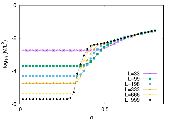
Figure 5: $Log_{10}\frac{M}{L^{2}}$ vs. $\sigma$ on an $L\times L$ honeycomb lattice for $0<\sigma\leq 0.8$ and different values of $L$. A comparison with Fig.3 indicates that critical hysteresis is absent on the honeycomb lattice (see text).

Simulations presented in Fig.4 demonstrate the existence of critical hysteresis on a triangular lattice. Of course, the result is not new diana ; kurbah ; janicevic , but it validates a new method. Our goal is to apply the new method to examine criticality on dilute triangular lattice and compare with previous results  kurbah . In preparation for this goal we apply the new method to the case $c=0$ as well, i.e. on a honeycomb lattice. Fig.5 shows the results. Earlier studies have indicated the absence of critical hysteresis on a honeycomb lattice  sabhapandit . Therefore any prominent difference between the trends of Fig.4 and Fig.5 may be used as a tool to detect the presence or absence of critical hysteresis on a dilute lattice. Interestingly both figures have some common features as well as some prominent differences. Both show a threshold $\sigma_{th}$ such that $M(\sigma<<\sigma_{th};L)=2$ and consequently $G(\sigma<<\sigma_{th};L)=\log_{10}2-2\log_{10}L$. Thus in both cases the set of $G(\sigma;L)$ graphs for different $L$ are widely separated for $\sigma<<\sigma_{th}$ and merge into each other for $\sigma>>\sigma_{th}$ as may be expected.

The prominent difference between Fig.4 and Fig.5 lies in the crossover from a set of widely separated curves at $\sigma<<\sigma_{th}$ to their merger into each other at $\sigma>>\sigma_{th}$. On the triangular lattice, the curves maintain their relative order in $L$ but on the honeycomb lattice they reverse it. In the case $c=1$ each curve changes from concave up to convex up at the inflexion point $\sigma_{c}(L)$. As $L$ increases, $\sigma_{c}(L)$ decreases. In contrast, on the honeycomb lattice we do not see any clear indication of a inflexion point or a concave up portion. The threshold value of $\sigma$ below which $M(\sigma;L)=2$ depends on $L$ and varies somewhat from one configuration of random fields to another. The average over different configurations makes the curve rounded in this region but otherwise $G(\sigma;L)$ rises sharply with increasing $\sigma$ as well as increasing $L$. The sharp rise of $M(\sigma;L)$ with $\sigma$ and $L$ causes the reversal of the ordering of $G(\sigma;L)$ with respect to $L$ before the curves merge into each other from below. This crossover takes place over a relatively narrow window $[0,\sigma]$ which shrinks further with increasing $L$ and moves towards lower $\sigma$. We take this to be a signature of the absence of criticality on finite lattices. It is plausible that in the limit $L\to\infty$, the flat and concave up portions of the curves in Fig.5 may shrink to zero resulting in convex up curves over the full range $\sigma>0$, but it is difficult to prove it numerically on lattice sizes studied here. The absence of critical hysteresis on a honeycomb lattice has been proven theoretically for an asymmetric distribution of the random field. It was shown if on-site quenched random fields are positive with the half-width of their distribution going to zero, $m(h)$ would increase smoothly from $-1$ to $1$ as $h$ increases from $-\infty$ to $J$. A similar argument can be used to prove that more than half spins in the system would have turned up continuously at $h=J$ for a Gaussian random field distribution. In other words, magnetization reversal would occur without a discontinuity as $\sigma\to 0$. Therefore critical hysteresis on the honeycomb lattice may be ruled out in the thermodynamic limit. Keeping in mind that finite size effects decrease logarithmically slowly, we take Fig.5 as showing the absence of criticality on the honeycomb lattice.

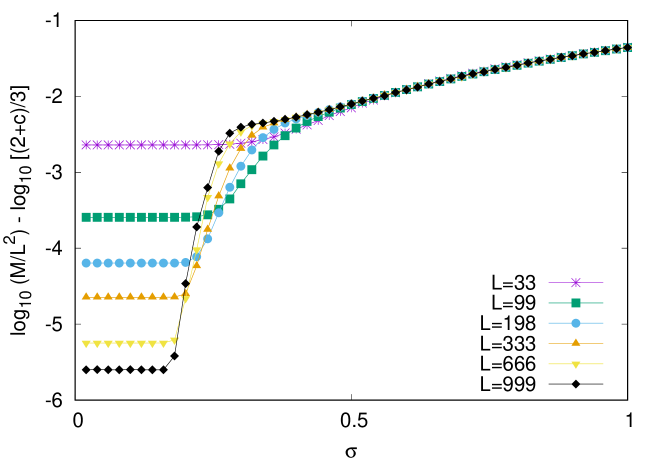
Figure 7: Metastable states vs. $\sigma$ on a partially diluted triangular lattice with $c=0.40$ in the range $0.1\leq\sigma\leq 1.0$.

The above discussion provides us a reasonable signature of critical hysteresis which can be read off from $G(\sigma;L)$ vs. $\sigma$ graphs. Fig.6, Fig.7, and Fig.8 show the results of simulations on dilute triangular lattice with $c=0.3,0.4$, and $0.6$ respectively. It is evident that the case $c=0.3$ as well as $c=0.4$ is similar to the case $c=0$. Thus we conclude that critical hysteresis is absent in these cases. The graphs for $c=0.6$ seem to have a mixed character. Results for $L=33,99,198$ have the features of $c=0$ while those for $L=333,666,999$ appear closer in character to $c=1$. To us it seems that lattice with $c=0.6$ supports critical hysteresis albeit it is a borderline case.

III Discussion and Concluding Remarks

Hysteresis in the zero-temperature random-field Ising model on honeycomb ($z=3$) and triangular ($z=6$) lattices is a difficult problem analytically as well as numerically. Extant work indicates that honeycomb lattice does not support critical hysteresis but the triangular lattice does so. However the critical point $\sigma_{c}(L)$ on the triangular lattice decreases extremely slowly with increasing system size $L$. Intensive numerical simulations on large systems ($N\approx 10^{10}$) have been used to estimate $\sigma_{c}$ in the limit $L\to\infty$. The problem on the dilute triangular lattice is even more challenging. Simulations on modest systems ($N\approx 10^{6}$) along with finite size scaling and percolation arguments predict $\sigma_{c}=0$ for $c<1/3$. At first sight this appears reasonable. It is similar to the behavior on Bethe lattices of uniform integer connectivity; $\sigma_{c}>0$ if $z\geq 4$. A dilute triangular lattice with $c<1/3$ corresponds to $z_{av}<4$ and one may expect it to have $\sigma_{c}=0$. However, recently obtained exact solutions of the model on non-integer Bethe lattices predict $\sigma_{c}>0$ for $3<z_{av}\leq 4$. If similarity between Bethe and periodic lattices were to hold in general, it would mean $\sigma_{c}>0$ on dilute triangular lattice for $0<c<1/3$ as well. The motivation for the present work was to examine this point.

We have used an approach based on the number of metastable states in the system $M(\sigma;L)$ and $G(\sigma;L)=\log_{10}M(\sigma;L)-2\log_{10}(L)$. For a random field distribution N(0,$\sigma^{2}$) on lattices of size $33\leq L\leq 999$ we find $G(\sigma;L)=\log_{10}2-2\log_{10}L$ in the range $0\leq\sigma\leq 0.3$. It rises monotonically towards zero in the limit $\sigma\to\infty$. The manner of rise depends on $c$ and indicates whether criticality is present or not. Drawing upon a general agreement in the literature that critical hysteresis exists for $c=1$ but not for $c=0$, we take the differences in the behavior of $G(\sigma;L)$ for these two cases as signatures of the presence or absence of criticality on a diluted lattice. The signatures are as follows. Consider $G(\sigma;L_{1})$ and $G(\sigma;L_{2})$ with $L_{2}>L_{1}$. At very small values of $\sigma$, we have $G(\sigma;L_{1})>G(\sigma;L_{2})$. If criticality is present this order is maintained as both graphs go from concave up to convex up at inflexion points $\sigma_{c}(L_{1})$ and $\sigma_{c}(L_{2})$ respectively. For $\sigma\geq\sigma_{c}(L_{1})$, $G(\sigma;L_{1})$ merges with $G(\sigma;L_{2})$ from above. If criticality is not present, the graphs do not show an inflexion point. Both appear convex up but $G(\sigma;L_{2})$ overtakes $G(\sigma;L_{1})$ before it merges with it from below for larger $\sigma$. These signatures are understandable consequences of the presence or otherwise of an infinite avalanche in the system. Apart from the absence of an infinite avalanche that causes $G(\sigma;L)$ to rise sharply with increasing $\sigma$, the connectivity $z$ of the lattice also plays a role. Lattices which do not support criticality have a lower connectivity e.g. $z=3$ for the honeycomb lattice. A typical avalanche on such lattice is smaller because there are lesser number of pathways going out from an unstable site to a potentially flippable site.

Somewhat unexpectedly the simulations presented here indicate $\sigma_{c}=0$ for $0<c<0.6$ approximately. We have used systems of the same order ($N\approx 10^{6}$) as used in  kurbah but processing of data under finite size scaling hypothesis has been avoided. The reason is that even if there is a theoretical argument for $\sigma_{c}\to 0$ as $L\to\infty$, a finite system would necessarily have an instability in the region $\sigma<\sigma_{th}$ where the first spin to flip up would cause all other spins to flip up as well. Fluctuations are extremely large in this region and finite-size scaling used in reference  kurbah may not be reliable. Fig.6-Fig.8 show that $\sigma_{th}$ is in the same ballpark as $\sigma_{c}$ predicted by finite size scaling in the range $0\leq c\leq 0.6$. Thus an alternate method used in the present paper may be more reliable and a correction in earlier results is warranted. We note that earlier results  kurbah also showed a change of behavior at $c\approx 0.6$. Table II and Fig.6 of reference  kurbah show a nearly linear decrease of $\sigma_{c}$ from $1.22$ at $c=1$ to $0.33$ at $c=0.6$; more rapid decrease to $0.26$ at $c=0.5$; then a constant value equal to $0.25$ at $c=0.40$ and $c=0.34$ before an abrupt drop to $0$ at $c=0.33$.

The change of behavior near $c=0.6$ and qualitative difference from dilute Bethe lattices most likely originates from closed loops on the diluted triangular lattice. It appears that closed loops on a lattice affect critical hysteresis more strongly than we expected beforehand. There are other indications as well. A square lattice is similar to a $z=4$ Bethe lattice in that both have the same connectivity and support critical hysteresis but $\sigma_{c}$ is quite different on the two lattices;$\sigma_{c}=0.54$ on a square lattice and $\sigma_{c}=1.78$ on a $z=4$ Bethe lattice. The difference is even more pronounced between a simple cubic and $z=6$ Bethe lattice. A diluted lattice has positional disorder as well as the random field. Although the average connectivity of the diluted lattice varies linearly with $c$ but the fraction of nodes with different connectivities vary differently with $c$. This possibly changes the nature of loops on the lattice. Our work suggests that positional disorder on a periodic lattice has a much stronger effect on $\sigma_{c}$ than it has on a Bethe lattice.

DT acknowledges the support from Institute for Basic Science in Korea (IBS-R024-D1).

Figure 2: Number of metastable states M $vs.$ $\sigma$ comprising the lower half of hysteresis loop on a triangular lattice of size $33\times 33$ for Gaussian random field distributions N[0,$\sigma^{2}$]; for each $\sigma$ the value of M is averaged over $10^{4}$ independent realizations of the distribution. The first inset on the left shows an enlarged view of the graph in the range $0<\sigma<4$. The second inset on the right shows the same data as in the first inset but on a logarithmic scale along the y-axis.

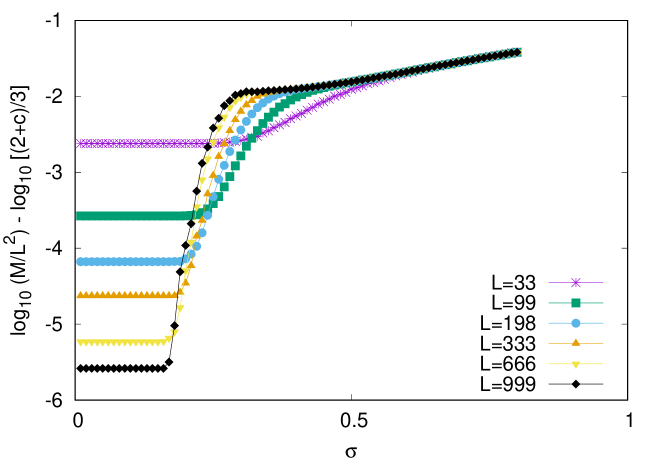
Figure 6: Metastable states vs. $\sigma$ on a partially diluted triangular lattice with $c=0.30$ in the range $0.1\leq\sigma\leq 0.8$.

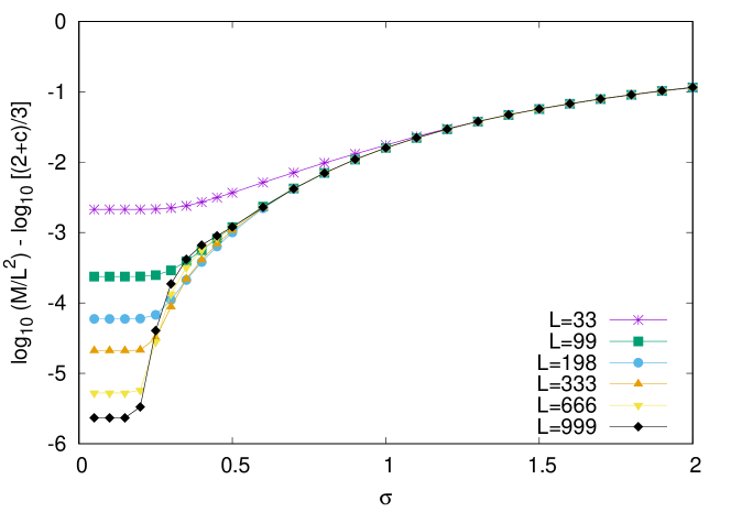
Figure 8: Metastable states vs. $\sigma$ on a partially diluted triangular lattice with $c=0.60$ in the range $0.1\leq\sigma\leq 2.0$.

References

- (1) Y Imry and S-k Ma, Phys Rev Lett 35, 1399 (1975).
- (2) E Ising, Z Phys 31, 253 (1925).
- (3) J Z Imbrie, Phys Rev Lett 53, 1747 (1984).
- (4) J P Sethna, K A Dahmen, S Kartha, J A Krumhansl, B W Roberts, and J D Shore, Phys Rev Lett 70, 3347 (1993).
- (5) O Percovic, K A Dahmen, and J P Sethna, Phys Rev B 59, 6106 (1999); arXiv:cond-mat/9609072 (1996).
- (6) J P Sethna, K A Dahmen, and C R Myers, Nature 410, 242 (2001), and references therein.
- (7) D Spasojevic, S Janicevic, and M Knezevic, Phys Rev Lett 106, 175701 (2011).
- (8) D Dhar, P Shukla, and J P Sethna, J Phys A30, 5259 (1997).
- (9) T P Handford, F J Peres-Reche, and S N Taraskin, Phys Rev E 87, 062122 (2013).
- (10) P Shukla and D Thongjaomayum, J Phys A: Math Theor 49, 235001 (2016).
- (11) P Shukla and D Thongjaomayum, Phys Rev E 95, 042109 (2017) and references therein.
- (12) S Sabhapandit, D Dhar, and P Shukla, Phys Rev Lett 88, 197202 (2002).
- (13) D Thongjaomayum and P Shukla, Phys Rev E 88, 042138 (2013).
- (14) S Janicevic, and M Mijatovic, and D Spasojevic, Phys Rev E 95, 042131 (2017).
- (15) L Kurbah, D Thongjaomayum, and P Shukla, Phys Rev E 91, 012131 (2015).
- (16) Prabodh Shukla, Phys Rev E 97, 062127 (2018).
- (17) Prabodh Shukla, Phys Rev E 98, 032144 (2018).