An Adaptive Observer Design for Charge-State and Crossover Estimation in Disproportionation Redox Flow Batteries undergoing Self-Discharge

Abstract

This article considers a model formulation and an adaptive observer design for the simultaneous estimation of the state of charge and crossover flux in disproportionation redox flow batteries. This novel nonaqueous battery chemistry allows a simple isothermal lumped parameter model to be formulated. The transport of vanadium through the porous separator is a key unknown function of battery variables and it is approximated in the space of continuous functions. The state and parameter observer adaptation laws are derived using Lyapunov analysis applied to the estimation error, the stability and convergence of which are proved. Numerical values of observer gains are calculated by solving a polytopic linear matrix inequality and equality problem via convex optimization. The performance of this design is evaluated on a laboratory flow battery prototype, and it is shown that the crossover flux can be considered a linear function of state of charge for this battery configuration during self-discharge.

I Introduction

Although redox flow batteries (RFBs) have become a promising alternative for grid-scale energy storage, many fundamental challenges have to be addressed to make them competitive. A persistent issue is the crossover of active species through the separator, which leads to electrolyte imbalance and capacity fade [1, 2, 3, 4].

To improve the design and management of RFBs, several multi-physics models have been developed, in particular for all-vanadium chemistries [5, 6, 7]. The pioneering studies commonly assume perfect membrane selectivity. More realistic distributed-parameter models usually include, in both porous electrodes and across the separator, species, charge, and momentum conservation, mass transport by diffusion, convection and migration, ohmic losses, and interfacial reaction kinetics [8, 9, 10, 11]. Alternatively, simpler and computationally-tractable lumped parameter approaches have been proposed, accounting for ion transport across the membrane through standard pseudo-steady transport assumptions, which establish species fluxes proportional to their concentration differences [12, 13, 14, 15].

All of these models involve parameters that are commonly assumed known, by means of standard experiments or model fits (e.g. [16]). In particular, the separator crossover flux, typically taken to be governed by Fickian diffusion [17, 18, 19, 20], is analyzed to quantify side reactions that consume the active species and consequently cause capacity fade [21, 10]. These models do not fully address the more complex transport behaviour of the membrane, for example caused by solute/solute interactions or microstructural effects [22, 23]. The resulting unmodeled dynamics, in addition to the assumption of invariance of the model parameters with respect to battery internal states, leads to erroneous long-term predictions of performance.

To account for the physico-chemical properties of the battery and their changes, model parameters are typically obtained either via experimental methods, or least squares regression approaches (see discussion in [24, 25]). Due to their simple practical implementation, real-time observer-based schemes for lumped parameter models of RFBs have also received attention [28, 29, 30, 31, 32]. These on-line identification methods are robust against uncertain initial conditions and can perform predictions of the main states of the battery based on a fixed set of parameters, or in some cases simultaneously provide their continuous estimation. In general, similar to the widespread on-line estimation methods for lithium-ion batteries [33], these approaches use electrical equivalent circuit models (ECMs) to emulate the RFB behaviour, and commonly perform the state/parameter estimation via the extended Kalman filter (EKF) [28, 34, 29, 32], amongst other model-based observer schemes [30, 31]. However, due to limitations in the formulation of the model, or convergence issues of the EKF, the crossover flux is not explicitly included in this type of approach.

This paper therefore addresses the challenge of simultaneous estimation of battery states and crossover flux for a novel type of nonaqueous RFB based on vanadium acetylacetonate disproportionation [35, 36]. This underlying chemistry allows a particularly simple isothermal lumped-parameter model to be employed for a disproportionation redox flow battery (DRFB). The model considers the state of charge in one half-cell and its associated electrolyte reservoir, alongside the crossover flux out of the half-cell through the separator. A general mathematical structure is used to express crossover flux, avoiding any assumptions particular to a given transport mechanism through the membrane.

To perform an on-line simultaneous estimation of the battery unknown states and parameters, an adaptive observer is designed via the standard Lyapunov second method of stability. From the analysis of the stability and convergence of the observer estimation error, a coupled Linear Matrix Inequalities and Equality (LMI-LME) problem is derived, which is numerically solved via convex optimization, using a polytopic approach.

I-A Notation

The space of all continuous functions on the domain $\Omega$ into $\mathbb{R}$ is denoted $\mathcal{C}(\Omega;\mathbb{R})$. The set of (symmetric) positive definite matrices of dimension $n\times n$ is denoted $\mathbb{S}^{n}_{+}$, and $I_{n}$ is the identity matrix of dimension $n\times n$. Also, $\mathbb{R}^{+}\equiv[0,+\infty)$, $\dot{v}(t)\triangleq\frac{dv}{dt}(t)$, $\|x\|\triangleq\sqrt{x^{\top}x}$ with $x\in\mathbb{R}^{n}$ being a real vector of dimension $n$, and $\|E\|\triangleq\sqrt{\lambda_{\text{max}}(E^{\top}E)}$ with $E$ being a real matrix, where $\lambda_{\text{max}}$ denotes the largest eigenvalue; $\lambda_{\text{min}}$ stands for the smallest eigenvalue.

II Modeling DRFBs

In a DRFB, identical liquid electrolyte solutions are stored in two separate reservoirs (see Figure 1), which contain a single metal electroactive species that can be both oxidized and reduced. When the battery is fully discharged, the active species in both reservoirs have identical oxidation states. The vanadium acetylacetonate ($\ce{V(acac)3}$) compound supports disproportionation electrochemistry.

Figure 1: Schematic of a DRFB using vanadium acetylacetonate

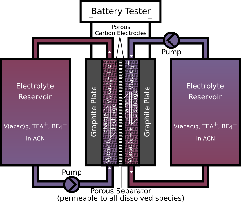
A typical V(acac)3 cell differs significantly from a traditional aqueous all-vanadium RFB. To access the high redox potential associated with V(acac)3 disproportionation, one must use a nonaqueous solvent whose electrochemical stability window is wider than water. The reversible nature of the disproportionation reaction means that the battery is tolerant to crossover, which impacts coulombic efficiency but does not permanently degrade charge capacity. This in principle enables use of porous separators, rather than costly ion-exchange materials, and opens up a value tradeoff between the reactor capital cost and its coulombic efficiency [3, 35, 23, 36, 37].

Cyclic voltammetry experiments [35] reveal two main redox couples associated with $\ce{V(acac)_{3}}$

$$\begin{split}&\bullet\quad\text{Negative Chamber}\\[-2.84544pt] &\ce{V(III)(acac)_{3}+e-<=>[charge][discharge][V(II)(acac)_{3}]^{-}},\\[-2.84544pt] &\bullet\quad\text{Positive Chamber}\\[-2.84544pt] &\ce{V(III)(acac)_{3}<=>[charge][discharge][V(IV)(acac)_{3}]^{+}+e^{-}},\end{split}$$

with an equilibrium cell potential of $E^{\text{0}}=$2.18 [V] [35, 23]. Crossover and the resulting self-discharge of the battery is due to the comproportionation of $\ce{V(II)}$ and $\ce{V(IV)}$ to form $\ce{V(acac)3}$ [23].

II-A Isothermal Lumped Parameter Model

Due to the symmetry inherent to disproportionation chemistry, the model analysis can be carried out by considering only one side of the battery. Let $n=n(t)$ be the amount of neutral $\ce{V(acac)_{3}}$ species remaining in one reservoir. In isothermal operation, its rate of change is due to the current $I$ driven by the battery, and the crossover flow $Q_{x}$ through the separator, namely

$$\frac{dn}{dt}(t) =\frac{I(t)}{\mathcal{F}}+Q_{x}(s(t)),$$ (1)

where $\mathcal{F}$ is Faraday’s constant and $s$ stands for some variables/states of the battery. Thus, for an initial amount of neutral $\ce{V(acac)_{3}}$ in the prepared solution $n_{0}$, considering the half-cell reactor volume $V_{\text{cell}}$ to be negligible with respect to the overall volume in the reservoir $V_{\text{res}}$, the state-of-charge of the overall system can be described by:

$$\begin{split}SOC(t)&=\frac{n_{0}-n(t)}{n_{0}}=\frac{c_{0}-c(t)}{c_{0}},\\ \frac{dSOC}{dt}(t)&=\!-\!\left(\frac{1}{c_{0}V_{\text{res}}}\right)Q_{x}(s(t))\!-\!\left(\frac{1}{c_{0}V_{\text{res}}\mathcal{F}}\right)I(t),\end{split}$$ (2)

with $c_{0}\!=\!n_{0}/V_{\text{res}}$ and $c(t)\!=\!n(t)/V_{\text{res}}$, being the initial and overall concentration of neutral species in the battery, respectively.

Similarly to a continuous stirred tank reactor model, we apply conservation of mass to one half-cell only, and assuming perfect mixing, this leads to

$$\frac{d\left(n_{\text{cell}}-n\right)}{dt}(t)=Q(t)\left(c(t)-c_{\text{cell}}(t)\right),$$

$$SOC_{\text{cell}}(t)=\frac{c_{0}-c_{\text{cell}}(t)}{c_{0}},$$ (3)

$$\frac{dSOC_{\text{cell}}}{dt}(t)=\!-\!\left(\frac{1}{\epsilon c_{0}V_{\text{cell}}}\right)\frac{dn}{dt}(t)\!-\!\left(\frac{Q(t)}{\epsilon V_{\text{cell}}}\right)\Delta SOC(t),$$

where $n_{\text{cell}}$ represents the amount of neutral $\ce{V(acac)_{3}}$ in the half-cell, $SOC_{\text{cell}}$ represents the state of charge in the reactor (which may be different from the overall SOC), and $Q$ stands for the volumetric flow rate in the reactor (considered measurable and equal in both chambers); $c_{\text{cell}}(t)\!=\!n_{\text{cell}}(t)/(\epsilon V_{\text{cell}})$ and $\Delta SOC(t)\!=\!SOC_{\text{cell}}(t)\!-\!SOC(t)$ with $\epsilon$ accounting for the known porosity of the carbon electrode. Thus, from (2)-(3), the resulting space-state isothermal lumped parameter model for the DRFB is

$$\begin{bmatrix}\frac{dSOC}{dt}(t)\\[2.84544pt] \frac{dSOC_{\text{cell}}}{dt}(t)\end{bmatrix}=\underbrace{\begin{bmatrix}0&0\\ \frac{Q(t)}{\epsilon V_{\text{cell}}}&-\frac{Q(t)}{\epsilon V_{\text{cell}}}\end{bmatrix}}_{A(Q(t))}\begin{bmatrix}SOC(t)\\ SOC_{\text{cell}}(t)\end{bmatrix}+$$

$$\underbrace{\begin{bmatrix}-\frac{1}{c_{0}V_{\text{res}}}\\[2.84544pt] -\frac{1}{\epsilon c_{0}V_{\text{cell}}}\end{bmatrix}}_{E}Q_{x}(s(t))+\underbrace{\begin{bmatrix}-\frac{1}{c_{0}V_{\text{res}}\mathcal{F}}\\[2.84544pt] -\frac{1}{\epsilon c_{0}V_{\text{cell}}\mathcal{F}}\end{bmatrix}}_{B}I(t),$$ (4)

$$V_{\text{out}}(t)=\underbrace{E^{\text{0}}_{\text{cell}}\!+\!\frac{2\mathcal{RT}}{\mathcal{F}}\ln{\left(\frac{SOC_{\text{cell}}(t)}{1\!-\!SOC_{\text{cell}}(t)}\right)}\!+\!V_{R}(t)}_{\Gamma(SOC_{\text{cell}}(t),I(t))},$$ (5)

where $V_{\text{out}}$ stands for the measurable output voltage of the battery in accordance with the Nernst equation, $\mathcal{R}$ is the universal gas constant, $\mathcal{T}\!=\!275\ ^{\circ}\text{K}$ and $V_{R}=V_{R}(SOC_{\text{cell}}(t),I(t))$ accounts for voltage drops due to overpotentials, likely caused by kinetic and resistive phenomena ($V_{R}(SOC_{\text{cell}}(t),0)=0$).

II-B General Approximate Model

Due to the nature of the electrochemical phenomena involved in RFBs, it can be considered that the unknown function for crossover flow $Q_{x}\!\in\!\mathcal{C}(\Omega;\mathbb{R})$, with $\Omega$ a compact set, and $s\!:\!\mathbb{R}^{+}\!\!\to\!\Omega$ a vector of $k\!\in\!\mathbb{N}$ battery variables, which could be states, inputs or outputs of the model, or even other measurements, independent of the model. Thus, using the universal approximation property of radial basis functions (RBFs) [38] or fuzzy inference systems [39] (in accordance with Stone-Weierstrass approximation theorem [40]),

$$Q_{x}(s(t))=\Psi(s(t))\theta+\varepsilon(s(t)),$$ (6)

$\forall\ t\!\in\![t_{i},t_{i+1}]_{i\in\mathbb{N}}$, with $\theta\!\in\!\mathbb{R}^{m}$ being a piece-wise constant vector of parameters and $\varepsilon$ an arbitrarily small approximation error in accordance with $m\!\in\!\mathbb{N}$ number of bounded basis functions $\psi_{j}\!:\!\overline{\Omega}\!\supseteq\!\Omega\!\to\!\mathbb{R}$ selected $\forall\ j\!\in\![0,m]$, where $\Psi\raisebox{0.85pt}{=}[\psi_{1},\ldots,\psi_{m}]$.

Let $x=[SOC,SOC_{\text{cell}}]^{\top}$ be the vector of battery states. Using the above-described approximation of the crossover function, (4)-(5) can be formulated as

$$\dot{x}(t)= A(Q(t))x(t)+E\Psi(s(t))\theta(t)+BI(t)+E\varepsilon(s(t)),$$

$$\dot{\theta}(t)= 0^{\top},\qquad\quad\forall\ t\in[t_{i},t_{i+1}],$$ (7)

$$y(t)= \Gamma^{-1}(V_{\text{out}}(t),I(t),V_{R}(t))=\overbrace{\begin{bmatrix}0&1\end{bmatrix}}^{C}x(t)+w(t),$$

with $x(0)\!=\!x_{0}$ and $\theta(0)\!=\!\theta_{0}$ being unknown state and parameter initial conditions, respectively, $y$ being the measurable battery output, $w$ the measurement error, and $\bigcup_{i\in\mathbb{N}}[t_{i},t_{i+1}]\!=\!\mathbb{R}^{+}$ for consecutive time intervals. This model, however, must satisfy the following conditions:

Condition 1.

The functional structure of the $V_{R}$ term in (5) is such that the non-linear mapping $\Gamma$ is globally invertible. In addition, due to errors in the measurements, the inversion of this mapping is such that $w$ in (7) is always bounded: $\sup_{t}\{\|w(t)\|\}\leq\bar{w}$, $\forall\ t\in\mathbb{R}^{+}$, for some $\bar{w}\in\mathbb{R}^{+}$.

Condition 2.

Crossover through the separator represents a slow degradation process such that in (7) there exist $[t_{i},t_{i+1}]$ finite time intervals $\forall\ i\!\in\!\mathbb{N}$, and bounded parameters: $\sup_{t}\{\|\theta(t)\|\}\leq\gamma_{\theta}$, which lead to a bounded approximation error: $\sup_{t}\{\|\varepsilon(s(t))\|\}\leq\bar{\varepsilon}$ in (6), $\forall\ t\in\mathbb{R}^{+}$, for some $\gamma_{\theta}\in\mathbb{R}^{+}$ and $\bar{\varepsilon}\in\mathbb{R}^{+}$.

Condition 3.

The vector of basis functions $\Psi$ in (6) is always bounded: $\sup_{t}\{\|\Psi(z(t))\|\}\leq\!\gamma_{\Psi}$, $\forall\ t\!\in\!\mathbb{R}^{+}$ and every vector function $z:\!\mathbb{R}^{+}\!\to\!\mathbb{R}^{k}$, with $\gamma_{\Psi}=\sup_{t\in\mathbb{R}^{+}}\{\|\Psi(z(t))\|\}\in\!\mathbb{R}^{+}$. In addition, this satisfies the Lipchitz condition with respect to the battery states/variables, namely $\|\Psi(s(t))\!-\!\Psi(\hat{s}(t))\|\leq\gamma_{\tilde{\Psi}}\|s(t)-\hat{s}(t)\|$, for some $\gamma_{\tilde{\Psi}}\!\in\!\mathbb{R}^{+}$, $\forall\ s\!:\!\mathbb{R}^{+}\to\Omega$ and $\hat{s}\!:\!\mathbb{R}^{+}\to\overline{\Omega}\supseteq\Omega$, $\forall\ t\in\mathbb{R}^{+}$.

Condition 4.

The volumetric flow rate $Q$ is a bounded measurable variable with $Q_{m}\!=\!\inf_{t}\{Q(t)\}>0$ and $Q_{M}\!=\!\sup_{t}\{Q(t)\}$, so that its domain of operation $\mathcal{Q}\!=\![Q_{\text{m}},Q_{\text{M}}]$ is a compact set known in advance. Thus, the time-varying matrix $A$ in (4) can always be embedded in a polytope of matrices $\mathcal{A}$ where

$$A(Q(t))\in\mathcal{A} =\mathbf{Co}\{A(Q_{\text{m}}),A(Q_{\text{M}})\}$$

$\forall\ t\in\mathbb{R}^{+}$, where $\mathbf{Co}$ denotes the convex hull (minimal convex polytope) [41, 42].

III Adaptive Observer Design

For the approximate model (7), the observer design can be carried out using Lyapunov stability theory [43] applied to state and parameter estimation of nonlinear uncertain systems [44, 45, 46, 47, 48, 49, 50]. The aim is to achieve stability in the sense of uniformly ultimately bounded (UUB) convergence of the observer estimation error.

III-A Adaptive Observer

An adaptive Luenberger-type observer [51] for simultaneous estimation of battery state and parameters for the system (7) has the structure

$$\dot{\hat{x}}(t) =A(Q(t))\hat{x}(t)+E\Psi(\hat{s}(t))\hat{\theta}(t)+BI(t)+L\tilde{y}(t),$$

$$\dot{\hat{\theta}}(t) =\Phi(\tilde{y}(t),\Psi(\hat{s}(t))),$$ (8)

$$\hat{y}(t) =C\hat{x}(t),$$

where $\hat{x}$, $\hat{\theta}$ and $\hat{y}$ are estimated states, parameters and outputs, respectively, $\hat{x}(0)\!=\!\hat{x}_{0}$ and $\hat{\theta}(0)\!=\!\hat{\theta}_{0}$ are estimated initial conditions, $\hat{s}$ stands for the estimated states/variables of the battery chosen to model the crossover flux, $\tilde{y}(t)\!=\!y(t)\!-\!\hat{y}(t)$ denotes the output estimation error, $L\in\mathbb{R}^{n}$ is the observer linear feedback gain and $\Phi$ is the adaptive compensation function to adapt parameters in (6) as the battery evolves.

III-B Observer Estimation Error

The dynamical error between the model (7) and the proposed observer (8) can be written as:

$$\begin{split}\dot{\tilde{x}}(t)&=\bar{A}(t)\tilde{x}(t)+E\eta(t)-Lw(t),\\ \eta(t)&=\tilde{\Psi}(t)\theta(t)+\hat{\Psi}(t)\tilde{\theta}(t)+\varepsilon(t)\\ \dot{\tilde{\theta}}(t)&=-\Phi(\tilde{y}(t),\hat{\Psi}(t)),\qquad\qquad\qquad\forall\ t\in[t_{i},t_{i+1}],\\ \tilde{y}(t)&=C\tilde{x}(t)+w(t),\end{split}$$ (9)

where $\tilde{x}(t)\!=\!x(t)\!-\!\hat{x}(t)$, $\tilde{\theta}(t)\!=\!\theta(t)\!-\!\hat{\theta}(t)$ and $\tilde{y}(t)\!=\!y(t)\!-\!\hat{y}(t)$ are estimation errors for states, parameters and outputs, respectively, $\tilde{x}(0)\!=\!\tilde{x}_{0}$ and $\tilde{\theta}(0)\!=\!\tilde{\theta}_{0}$ are initial error conditions; $\tilde{\Psi}(t)\!\triangleq\!\Psi(s(t))\!-\!\Psi(\hat{s}(t))$, $\hat{\Psi}(t)\!\triangleq\!\Psi(\hat{s}(t))$ and $\varepsilon(t)\triangleq\varepsilon(s(t))$; $\bar{A}(t)\triangleq A(Q(t))-LC$ is the closed-loop compensated matrix.

Property 1.

Given the error dynamic (9), the expression

$$\delta(t) =PE\left((1-\rho)\tilde{\Psi}(t)\theta(t)+\varepsilon(t)\right)-Zw(t)$$ (10)

represents part of the uncertain dynamic which cannot be compensated by the observer feedback gain nor adaptive function in (8), with $P\in\mathbb{S}^{n}_{+}$, $Z\in\mathbb{R}^{n}$ and for some $\rho\in[0,1]$. If Conditions 1-3 are satisfied, the following upper bound hold:

$$\|\delta(t)\| \leq\sup_{t\in\mathbb{R}^{+}}\{\|\delta(t)\|\},$$

$$\leq\|PE\|\left(2(1-\rho)\gamma_{\Psi}\gamma_{\theta}+\bar{\varepsilon}\right)+\|Z\|\bar{w}=\bar{\delta},$$

$\forall\ t\in\mathbb{R}^{+}$, where the boundedness of the basis functions selected plays a relevant role.

III-C Observer Feedback Gain and Adaptation Law

Lemma 1.

Let $\upsilon(t)\triangleq\rho E\tilde{\Psi}(t)\theta(t)$ be a bounded signal for some $\rho\in[0,1]$, and state-variables $s$ in (6) be such that $\|\tilde{s}\|\leq\gamma_{\tilde{s}}\|\tilde{x}\|$ for some $\gamma_{\tilde{s}}\in\mathbb{R}^{+}$. If Conditions 2-3 are satisfied and $\alpha\in\mathbb{R}^{+}$ and $\beta\in\mathbb{R}^{+}$ are properly selected so that $\gamma^{2}\leq\alpha\beta$, then the following inequality holds:

$$2\tilde{x}(t)^{\top}P\upsilon(t) \leq\tilde{x}(t)^{\top}\left(\alpha PP+\beta I_{n}\right)\tilde{x}(t),$$

where $P\in\mathbb{S}^{n}_{+}$ and $\gamma\!=\!\rho\gamma_{E}\gamma_{\theta}\gamma_{\tilde{\Psi}}\gamma_{\tilde{s}}$ with $\gamma_{E}\!=\!\|E\|$, $\forall\ s\!:\!\mathbb{R}^{+}\to\Omega$, $\forall\ \hat{s}\!:\!\mathbb{R}^{+}\to\overline{\Omega}\supseteq\Omega$ and $\forall\ t\in\mathbb{R}^{+}$.

Proof.

Following similar arguments described in [52, 49], based on the binomial property $(\sqrt{\alpha}\|\tilde{x}^{\top}\!P\|\!-\!\sqrt{\beta}\|\tilde{x}\|)^{2}$ $=\!\alpha\|\tilde{x}^{\top}\!P\|^{2}\!+\!\beta\|\tilde{x}\|^{2}\!-\!2\sqrt{\alpha\beta}\|\tilde{x}^{\top}\!P\|\|\tilde{x}\|\geq\!0$, using bounds stated in Conditions 2-3 and considering $\|\tilde{s}\|\leq\!\gamma_{\tilde{s}}\|\tilde{x}\|$, the selection of $\alpha$ and $\beta$ such that $\gamma^{2}\leq\alpha\beta$ yields

$$2\tilde{x}^{\top}Pv(t) \leq 2\|\tilde{x}^{\top}P\|\|v(t)\|\leq 2\rho\|\tilde{x}^{\top}P\|\|E\|\|\tilde{\Psi}\|\|\theta\|,$$

$$\leq 2\rho\gamma_{E}\gamma_{\theta}\gamma_{\tilde{\Psi}}\|\tilde{x}^{\top}P\|\|\tilde{s}\|\leq 2\sqrt{\alpha\beta}\|\tilde{x}^{\top}P\|\|\tilde{x}\|,$$

$$\leq\alpha\|\tilde{x}^{\top}P\|^{2}+\beta\|\tilde{x}\|^{2}=\tilde{x}^{T}(\alpha PP+\beta I_{n})\tilde{x}.$$

Theorem 1.

Let Conditions 1-3 be satisfied by (7). If some positive constants $\alpha$ and $\beta$ are chosen such that $\alpha\beta\geq\gamma^{2}$ and the solution for the coupled Linear Matrix Inequality and Equality problem:

$$\begin{bmatrix}\raisebox{0.85pt}{-}\!A(Q(t))^{\top}\!P\raisebox{0.85pt}{-}PA(Q(t))\!+\!C^{\top}\!Z^{\top}\!+\!ZC\raisebox{0.85pt}{-}\beta I_{n}\raisebox{0.85pt}{-}W&\!\!\!\sqrt{\alpha}P\\ \sqrt{\alpha}P&\!\!\!I_{n}\end{bmatrix}\!\succeq\!0,$$

$$\ PE\!-\!C^{\top}F=0,$$ (11)

exists for some $P\in\mathbb{S}^{n}_{+}$, $W\!\succeq\!\textrm{diag}(\omega)$, $\omega\!\in\!\mathbb{R}^{n}$ ($\omega_{j}\!>0\!\ ,\forall j\!=\!1,\ldots,n,\omega_{i}\!>0\!\ ,\forall i\!=\!1,\ldots,n$), $Z\in\mathbb{R}^{n}$ and $F\in\mathbb{R}$, $\forall\ Q\in\mathcal{Q}$, then the adaptive observer (8) using the feedback gain and adaptation function

$$L =P^{-1}Z,$$ (12)

$$\Phi(\tilde{y}(t),\hat{\Psi}(t)) =\Lambda^{-1}\left(\hat{\Psi}^{\top}F\tilde{y}(t)-\frac{1}{2}\sigma\hat{\theta}\|\tilde{y}(t)\|\right),$$ (13)

respectively, for some $\sigma\in\mathbb{R}^{+}$ and $\Lambda\in\mathbb{S}^{m}_{+}$, guarantees that the state estimation error $\tilde{x}$ and the parameter estimation error $\tilde{\theta}$ have a UUB dynamic [43, pp. 168, 346].

Proof.

Let $V\!=\!\tilde{x}^{\top}\!P\tilde{x}+\tilde{\theta}^{\top}\!\Lambda\tilde{\theta}$ be a Lyapunov function candidate. Its time derivative along the trajectory (9) yields

$$\dot{V}=\ \tilde{x}^{\top}\!\left(\bar{A}(t)\!^{\top}\!P\!+\!P\bar{A}(t)\right)\tilde{x}\!+\!2\tilde{x}^{\top}PE\eta(t)\ +$$

$$2\dot{\tilde{\theta}}^{\top}\Lambda\tilde{\theta}-2\tilde{x}^{\top}PLw(t).$$ (14)

If the signal $\eta$ in (9) is decomposed by factor $\rho\in[0,1]$, then $\eta=\eta_{0}+(1-\rho)\tilde{\Psi}\theta+\hat{\Psi}\tilde{\theta}+\varepsilon$, where $\eta_{0}=\rho\tilde{\Psi}\theta$ represents the uncertain term which can be compensated by the observer feedback term $L\tilde{y}(t)$ in (8). Thus, considering (12) so that $\bar{A}(t)=A(Q(t))\!-\!P^{-1}ZC$, (14) can be written as

$$\dot{V}=\tilde{x}^{\top}\left(A(Q(t))^{\top}P+PA(Q(t))\!-\!C^{\top}Z^{\top}\!-\!ZC\right)\tilde{x}+$$

$$\underbrace{2\tilde{x}^{\top}PE\hat{\Psi}\tilde{\theta}+2\dot{\tilde{\theta}}^{\top}\Lambda\tilde{\theta}}_{T_{1}}+\underbrace{2\tilde{x}^{\top}P(\rho E\tilde{\Psi}\theta)}_{T_{2}}+2\tilde{x}^{\top}\delta(t).$$ (15)

Based on the LME condition in (11), substituting (13) into (15) and considering bounds from Conditions 1-3, the term $T_{1}$ can be upper bound by:

$$T_{1}= \ 2\tilde{x}^{\top}C^{\top}\!F\hat{\Psi}\tilde{\theta}\raisebox{0.85pt}{-}2\big{(}\Lambda^{-1}[\hat{\Psi}^{\top}F\tilde{y}\raisebox{0.85pt}{-}(1/2)\sigma\hat{\theta}\|\tilde{y}\|]\big{)}^{\top}\!\Lambda\tilde{\theta},$$

$$= \ \sigma\|C\tilde{x}+w\|(\theta-\tilde{\theta})^{\top}\tilde{\theta}\!-\!2w^{\top}F(\Psi\!-\!\tilde{\Psi})\tilde{\theta},$$

$$\leq \ \sigma\gamma_{C}\|\tilde{x}\|(\gamma_{\theta}\|\tilde{\theta}\|-\|\tilde{\theta}\|^{2})+2\gamma_{F}\gamma_{\tilde{\Psi}}\|w\|\|\tilde{x}\|\|\tilde{\theta}\|+$$

$$\ \sigma\|w\|(\gamma_{\theta}\|\tilde{\theta}\|-\|\tilde{\theta}\|^{2})+|-w^{\top}F\Psi\tilde{\theta}|,$$ (16)

$$\leq \ \sigma\gamma_{C}\|\tilde{x}\|\Big{(}\overbrace{\Big{[}\gamma_{\theta}+\frac{2\gamma_{F}\gamma_{\tilde{\Psi}}}{\sigma\gamma_{C}}\bar{w}\Big{]}}^{\gamma_{1}}\|\tilde{\theta}\|-\|\tilde{\theta}\|^{2}\Big{)}+$$

$$\ \sigma\bar{w}\Big{(}\underbrace{\Big{[}\gamma_{\theta}+\frac{2\gamma_{F}\gamma_{\Psi}}{\sigma}\Big{]}}_{\gamma_{2}}\|\tilde{\theta}\|-\|\tilde{\theta}\|^{2}\Big{)},$$

where $\gamma_{C}\!=\!\|C\|$ and $\gamma_{F}\!=\!\|F\|$. With respect to the term $T_{2}$, by virtue of Lemma 1 for the positive constants $\alpha$, $\beta$ so that $\gamma^{2}\leq\alpha\beta$ and Property 1, this leads to:

$$\dot{V}\!\leq\!\tilde{x}^{\top}\!\Big{(}\underbrace{\!A(Q(t))^{\top}\!P\raisebox{0.85pt}{+}PA(Q(t))\raisebox{0.85pt}{-}C^{\top}\!Z^{\top}\!\raisebox{0.85pt}{-}ZC\raisebox{0.85pt}{+}\alpha PP\raisebox{0.85pt}{+}\beta I_{n}}_{T_{3}}\!\Big{)}\tilde{x}$$

$$\raisebox{0.85pt}{+}\sigma\gamma_{C}\|\tilde{x}\|\left(\!\gamma_{1}\|\tilde{\theta}\|\raisebox{0.85pt}{-}\|\tilde{\theta}\|^{2}\right)\raisebox{0.85pt}{+}\sigma\bar{w}\left(\!\gamma_{2}\|\tilde{\theta}\|\raisebox{0.85pt}{-}\|\tilde{\theta}\|^{2}\right)\raisebox{0.85pt}{+}\ 2\|\tilde{x}\|\bar{\delta}.$$ (17)

Imposing the condition $T_{3}(t)\!\leq\!-W$, for some $W\!\succeq\!\textrm{diag}(\omega)$, $\omega\!\in\!\mathbb{R}^{n}$ ($\omega_{i}\!>0\!\ ,\forall i\!=\!1,\ldots,n$) and $\forall\ t\in\mathbb{R}^{+}$, a Riccati-like inequality is posed [52] which, by means of the Schur complement [41, 47], can be transformed to the constrained time-variant problem (11), convex in terms of the variables $\{P,Z,F,W\}$. If this problem is feasible, (17) can be written as:

$$\dot{V} \leq-\varrho\gamma_{W}\|\tilde{x}\|^{2}-\sigma\gamma_{C}\|\tilde{x}\|\left(\|\tilde{\theta}\|\!-\!\frac{\gamma_{1}}{2}\right)^{2}-\sigma\bar{w}\|\tilde{\theta}\|\left(\|\tilde{\theta}\|-\gamma_{2}\right)$$

$$\ -\|\tilde{x}\|\left((1-\varrho)\gamma_{W}\|\tilde{x}\|-\frac{\sigma\gamma_{C}\gamma_{1}^{2}}{4}-2\bar{\delta}\right),$$ (18)

with $\gamma_{W}=\lambda_{\text{min}}(W)$, for some $\varrho\in[0,1]$, so that (18) is negative defined outside of the ball $B=B(0,[r_{\tilde{x}},r_{\tilde{\theta}}])$ set forth by the radii:

$$\begin{split}\|\tilde{x}\|&\geq\frac{1}{4(1-\varrho)\gamma_{W}}\left(\sigma\gamma_{C}\gamma_{1}^{2}+8\bar{\delta}\right)=r_{\tilde{x}},\\ \|\tilde{\theta}\|&\geq\max\left\{\gamma_{2},\frac{\gamma_{1}}{2}+\left(\frac{\gamma_{1}^{2}}{4}+\frac{2\bar{\delta}}{\sigma\gamma_{C}}\right)^{1/2}\right\}=r_{\tilde{\theta}}.\end{split}$$ (19)

Therefore, according to the standard Lyapunov theorem: $\|\tilde{x}\|$ and $\|\tilde{\theta}\|$ have a convergent dynamic which is UUB [46, 53, 43, 54].

Remark 1.

Under the ideal situation of $\delta\!=\!0$ in ((10)), zero output measurement error ($w\!=\!0$) and $\sigma=0$, the equilibrium point $(\tilde{x},\tilde{\theta})\!=\!0^{\top}$ is uniformly stable and $\lim_{t\to\raisebox{0.85pt}{+}\infty}\tilde{x}(t)\to 0$ can be proved on the basis of Barbalat’s lemma. However, as is well-known, the convergence of the parameters to their actual values is only guaranteed under persistent excitation conditions, namely $c_{0}I_{n}\geq\int_{t_{0}}^{t_{0}+\Delta t}\Psi(s(\tau))\Psi(s(\tau))^{\top}d\tau\geq c_{1}I_{n}$, for some $\Delta t\in\mathbb{R}^{+}$, $c_{0}\in\mathbb{R}^{+}$ and $c_{1}\in\mathbb{R}^{+}$ [54, 55, 49].

III-D Polytopic Design Approach

Considering that the volumetric flow rate in (4) satisfies Condition 4, the approximate model (7) admits a polytope description so that the time-variant nature of the LMI-LME problem (11) can be recast as a polytopic convex problem [49, 42, 50, 41]:

$$\min_{\bar{\alpha},\gamma_{Z},\gamma_{F}}\left\{\bar{\alpha}+\kappa_{Z}\gamma_{Z}+\kappa_{F}\gamma_{F}\right\},$$ (20)

subject to:

$$\forall\ i\raisebox{0.85pt}{=}1,2\!:\!\left\{\!\!\!\begin{array}[]{l}\begin{bmatrix}\!-\!A^{\top}_{i}P\!-\!PA_{i}\!+\!C^{\top}Z^{\top}\!+\!ZC\!-\!\overline{W}&P\\ P&\bar{\alpha}I_{n}\end{bmatrix}\succeq 0,\end{array}\right.$$ (22)

$$\qquad\qquad\ \begin{bmatrix}\gamma_{Z}I_{n}&Z\\ Z^{\top}&\gamma_{Z}\end{bmatrix}\succeq 0,\ \begin{bmatrix}\gamma_{F}&F\\ F&\gamma_{F}\end{bmatrix}\succeq 0,$$

$$\qquad\qquad\ \ P=P^{\top}\succeq 0,W\succeq\text{diag}(\omega_{1},\ldots,\omega_{n}),$$

$$\qquad\qquad\ \ PE-C^{\top}F=0,$$

$$\qquad\qquad\ \ \bar{\alpha}>0,\gamma_{Z}\geq 0,\gamma_{F}\geq 0,$$

with $A_{1}=A(Q_{m})$ and $A_{2}=A(Q_{M})$ vertices of the convex hull $\mathcal{A}$, $\omega_{j}\!>0\!\ ,\forall j\!=\!1,\ldots,n$; $\bar{\alpha}=1/\alpha$ degree of freedom to maximise the uncertainty allowed by the LMI-LME (11), for a given $\beta$ and provided its feasible solution $\{P,Z,F,W\}$, with $\overline{W}=\beta I_{n}+W$. The constants $\kappa_{Z}\!\geq\!0$ and $\kappa_{F}\!\geq\!0$ are selected to adjust norm bounds of matrices $Z$ and $F$, respectively.

Remark 2.

In the crossover approximation (6) and consequent Lyapunov analysis of the observer estimation error (9), the basis functions are not necessarily dependent on the measurable output variable. If this is the case, for zero output measurement error ($w\!=\!0$), the LMI-LME problem (11) can be solved via a polytopic formulation of the Strictly Positive Real (SPR) condition on the resulting error dynamic [54].

IV RFB Experimental Methods

The self-discharge experiment was performed inside an argon-filled glovebox (PureLab, Inert Technologies, USA) with 0.1 M vanadium acetylacetonate (V(acac)₃, 98%, Strem, UK) as the active species dissolved in anhydrous acetonitrile (ACN, 99.8%, Sigma, UK) dried over molecular sieves (3 Å, Sigma-Aldrich, USA) with 0.2 M tetraethylammonium tetrafluoroborate (TEABF₄, Sigma, 99%, UK) used as a supporting salt.

A flow cell designed for nonaqueous electrolytes was used with 2.20 cm² of active area and reservoir volumes of 18 mL each. The flowrate of 9 mL/min corresponds to a reactor residence time of 4.65 s when using electrodes with a porosity $\epsilon$ of 0.87. Porous carbon felt electrodes (Alfa-Aesar, UK) compressed 50% to a final thickness of 3.17 mm were used in a flow-through configuration alongside impervious bipolar graphite plates (GraphiteStore, USA). A polypropylene porous separator (Celgard 4650, Celgard, USA) was used to separate the counter-current electrolyte flow inside the cell.

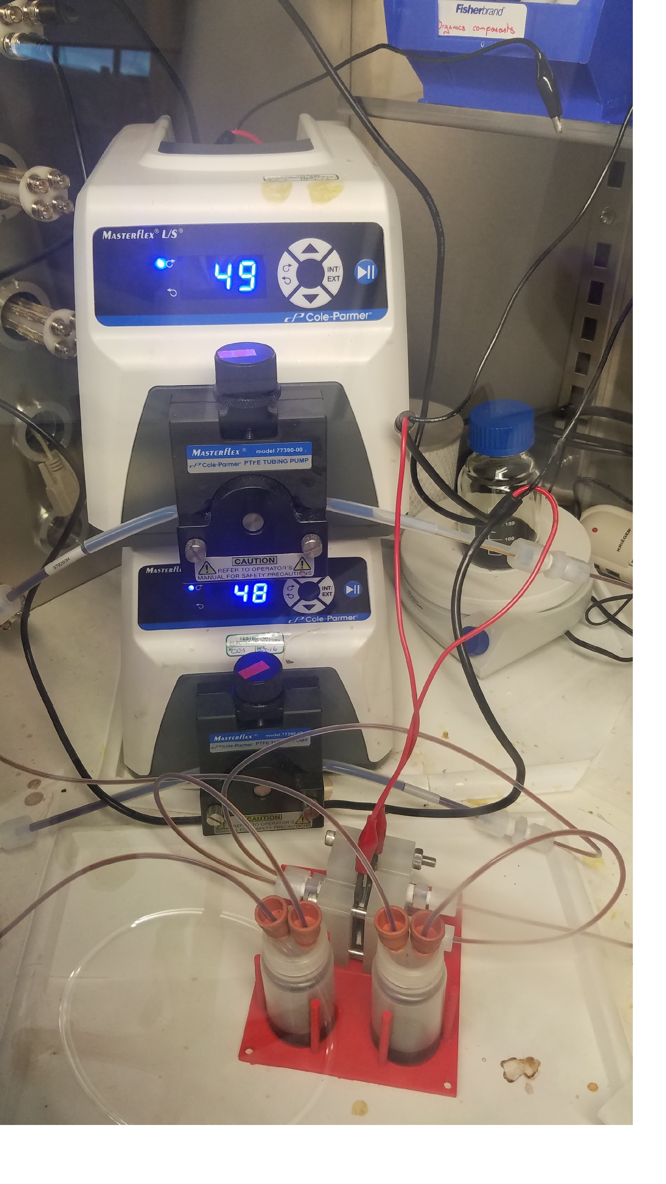
Peristaltic pumps (MasterFlex, Cole-Palmer, USA) circulated electrolyte through the half-cells using polytetrafluoroethylene (PTFE) tubing with perfluoroalkoxy alkane (PFA) compression fittings. Wetted materials in the system consisted entirely of PTFE, PFA, polypropylene, impervious graphite, and carbon felt. Figure 2 shows the operating experimental setup previously detailed.

Figure 2: RFB experiment running in glovebox

V Experimental Results

The flow battery was cyled between 3 V and 1 V three times at 20 mA/cm² with a battery tester (MACCOR 4000 series, USA) to precondition the system before charging to the 3 V voltage cutoff and letting the battery self-discharge at open circuit. Values of the experimental parameters in the model (4)-(5) are provided in Table I.

For comparison and validation purposes, the following linear function for the crossover term in (4) has been considered:

$$Q_{x}(SOC_{\text{cell}}(t))=k_{\text{mt}}\ c_{0}\overbrace{\left(\frac{c_{0}-c_{\text{cell}}(t)}{c_{0}}\right)}^{SOC_{\text{cell}}(t)},$$ (23)

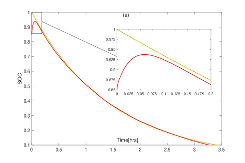
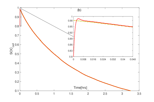
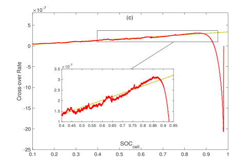
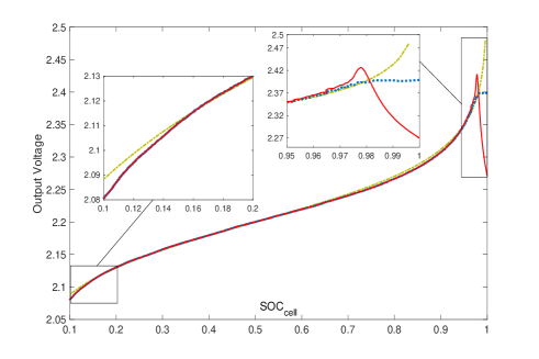
where $k_{\text{mt}}\!=\!5.6142\!\cdot\!10^{\!-8\!}$ L/min is the mass-transfer coefficient, a proposed constant which describes the expected linear relationship between $SOC_{\text{cell}}$ and $Q_{x}$. This value for $k_{mt}$ was calculated by fitting the model, (4)-(5), including (23), to the experimental data assuming an initial condition of 100% $SOC_{\textrm{cell}}$ at the beginning of the experiment and 50% $SOC_{\textrm{cell}}$ when the output voltage of the battery reached the equilibrium voltage of 2.2 V. Figure 3 illustrates the model-predicted internal battery states and mass-transfer term, respectively (dash-dot lines). Figure 4 depicts the model voltage output as a function of the predicted $SOC_{\textrm{cell}}$, which is mostly in good agreement with its measured value (dotted line), with the exception of the extreme zones of $SOC_{\textrm{cell}}$, where unmodeled dynamics in the argument of the Nernst equation (5) are expected to be present.

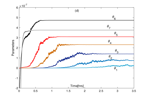
Regarding the proposed on-line adaptive observer (8), $\hat{x}_{0}\!=\![0.85,0.8]^{\top}$ and $\hat{\theta}_{0}\!=\!0^{\top}$ have been selected as its initial conditions. For the crossover approximation (6), $s\!=\!SOC_{\text{cell}}$, $\Omega\!=\![0,1]$ and seven ($m\!=\!7$) normalized radial basis functions, uniformly centred in $[0.05,0.95]$ with variance $0.0081$, have been considered. With respect to the observer gains in (12)-(13), $\Lambda^{\!-\!1}\!=\!4.798\!\cdot\!10^{\!-\!7}I_{7}$ and $\sigma\!=\!0.1$ have been selected to obtain to a slow parameter adaptation. The numerical solution of the polytopic LMI-LME problem (20), considering $Q_{\text{m}}\!=\!0.9Q$, $Q_{\text{M}}\!=\!1.1Q$, $\beta=10^{\!-\!4}$, $\kappa_{F}\!=\!10^{\!-\!5}$ and $\kappa_{Z}\!=\!1$, has been obtained via the Yalmip toolbox for Matlab [56] using the SDP package part of the Mosek solver [57]. More details about its Matlab code implementation and data can be found in [58]. The simultaneous estimation of the state-of-charge and crossover flux is shown in Figure 3 (solid lines), achieving similar behaviour to the aforementioned model (4)-(5)-(23). In particular, the estimated crossover flux, whose parameter convergence to stationary values is shown in 3(d), is in agreement with the linear relationship proposed in (23). Figure 4, solid lines, illustrates the accurate on-line predicted output voltage based on the estimated states provided by the adaptive observer.

Symbol	Description	Value	Units
$V_{\text{res}}$	Reservoir volume	17.6	mL
$V_{\text{cell}}$	Half-cell volume	0.6985	mL
$c_{0}$	Initial concentration $\ce{V(acac)3}$	$0.1$	mol/L
$Q$	Volumetric flow rate	9.0	mL/min
$\epsilon$	Porosity of carbon electrode	$0.87$	–
$E^{0}_{\text{cell}}$	Equilibrium cell potential	$2.2$	V

TABLE I: Parameters values for RFB experiment

Figure 3: Battery model (4)-(5) results with constant parameters in (23) (dash-dotted lines), alongside adaptive observer estimate (solid lines) for: (a) overall state-of-charge; (b) state-of-charge of the half-cell; (c) crossover flux; (d) estimated parameters of approximation (6).

Figure 4: Voltages with respect to cell state-of-charge, including: measured voltage response (dotted line); battery model (4)-(5) with constant parameters in (23) (dash-dotted line); and adaptive observer estimate (solid line).

VI Concluding Remarks

In this article an isothermal lumped model of a disproportionation redox flow battery and a related adaptive observer design have been presented. The design of the observer linear feedback gain and parameter adaptation law is based on Lyapunov stability theory and carried out by solving a polytopic LMI-LME problem. This provides a systematic methodology where the UUB convergence of state and parameter estimation errors is guaranteed. The crossover term has been approximated via radial basis functions, enabling continual estimation of the crossover flux as the battery discharges, which can then can be used predictively. A linear relationship between crossover flux and $SOC_{\textrm{cell}}$, captured by mass-transfer coefficient $k_{\textrm{mt}}$, is typically built into simple lumped-parameter RFB models, which assume pseudo-steady diffusion across a planar separator. In the adaptive observer, this relationship is not assumed, yet the observer reveals this linear dependence, as seen in Figure 3. Data from a vanadium acetylacetonate DRFB undergoing self-discharge was analyzed, demonstrating the observer’s capability to estimate state-of-charge and crossover simultaneously.

VII Acknowledgments

This work was carried out with funding support received from the Faraday Institution (faraday.ac.uk; EP/S003053/1), grant number FIRG003.

References

- [1] Puiki Leung, Xiaohong Li, Carlos Ponce de León, Leonard Berlouis, C. T. John Low, and Frank C. Walsh. Progress in redox flow batteries, remaining challenges and their applications in energy storage. RSC Adv., 2:10125–10156, 2012.
- [2] Massimo Guarnieri, Paolo Mattavelli, Giovanni Petrone, and Giovanni Spagnuolo. Vanadium redox flow batteries, potentials and challenges of a emerging storage technology. IEEE Industrial Electronics Magazine, 10(4):20–31, 2016.
- [3] Rebecca A. Potash, James R. McKone, Sean Conte, and Héctor D. Abruña. On the benefits of a symmetric redox flow battery. Journal of The Electrochemical Society, 163(3):A338–A344, 2016.
- [4] Xianfeng Li, Huamin Zhang, Zhensheng Mai, Hongzhang Zhang, and Ivo Vankelecom. Ion exchange membranes for vanadium redox flow battery (vrb) applications. Energy Environ. Sci., 4:1147–1160, 2011.
- [5] Adam Z. Weber, Matthew M. Mench, Jeremy P. Meyers, Philip N. Ross, Jeffrey T. Gostick, and Qinghua Liu. Redox flow batteries: a review. Journal of Applied Electrochemistry, 41(10):1137–1164, Sep 2011.
- [6] Q. Xu and T.S. Zhao. Fundamental models for flow batteries. Progress in Energy and Combustion Science, 49:40–58, 2015.
- [7] Q. Zheng, X. Li, Y. Cheng, G. Ning, F. Xing, and F. Zhang. Development and perspective in vanadium flow battery modeling. Applied Energy, 132:254–266, 2014.
- [8] A.A. Shah, H. Al-Fetlawi, and F.C. Walsh. Dynamic modelling of hydrogen evolution effects in the all-vanadium redox flow battery. Electrochimica Acta, 55(3):1125 – 1139, 2010.
- [9] Ching Liang Chen, Hak Koon Yeoh, and Mohammed Harun Chakrabarti. An enhancement to vynnycky’s model for the all-vanadium redox flow battery. Electrochimica Acta, 120:167 – 179, 2014.
- [10] K. W. Knehr, Ertan Agar, C. R. Dennison, A. R. Kalidindi, and E. C. Kumbur. A transient vanadium flow battery model incorporating vanadium crossover and water transport through the membrane. Journal of The Electrochemical Society, 159(9):A1446–A1459, 2012.
- [11] Yun Wang and Sung Chan Cho. Analysis and three-dimensional modeling of vanadium flow batteries. Journal of The Electrochemical Society, 161(9):A1200–A1212, 2014.
- [12] Ao Tang, Jie Bao, and Maria Skyllas-Kazacos. Dynamic modelling of the effects of ion diffusion and side reactions on the capacity loss for vanadium redox flow battery. Journal of Power Sources, 196(24):10737–10747, 2011.
- [13] A. A. Shah, R. Tangirala, R. Singh, R. G. A. Wills, and F. C. Walsh. A dynamic unit cell model for the all-vanadium flow battery. Journal of The Electrochemical Society, 158(6):A671–A677, 2011.
- [14] Maria Skyllas-Kazacos and Leesean Goh. Modeling of vanadium ion diffusion across the ion exchange membrane in the vanadium redox battery. Journal of Membrane Science, 399-400:43 – 48, 2012.
- [15] Philipp A. Boettcher, Ertan Agar, C. R. Dennison, and E. Caglan Kumbur. Modeling of ion crossover in vanadium redox flow batteries: A computationally-efficient lumped parameter approach for extended cycling. Journal of The Electrochemical Society, 163(1):A5244–A5252, 2016.
- [16] Y. Ashraf Gandomi, D. S. Aaron, J. R. Houser, M. C. Daugherty, J. T. Clement, A. M. Pezeshki, T. Y. Ertugrul, D. P. Moseley, and M. M. Mench. Critical review—experimental diagnostics and material characterization techniques used on redox flow batteries. Journal of The Electrochemical Society, 165(5):A970–A1010, 2018.
- [17] D. Schmal, J. Van Erkel, and P. J. Van Duin. Mass transfer at carbon fibre electrodes. Journal of Applied Electrochemistry, 16(3):422–430, May 1986.
- [18] E. Wiedemann, A. Heintz, and R.N. Lichtenthaler. Transport properties of vanadium ions in cation exchange membranes:: Determination of diffusion coefficients using a dialysis cell. Journal of Membrane Science, 141(2):215 – 221, 1998.
- [19] Chenxi Sun, Jian Chen, Huamin Zhang, Xi Han, and Qingtao Luo. Investigations on transfer of water and vanadium ions across nafion membrane in an operating vanadium redox flow battery. Journal of Power Sources, 195(3):890–897, 2010.
- [20] Jovan Kamcev, Donald R. Paul, Gerald S. Manning, and Benny D. Freeman. Accounting for frame of reference and thermodynamic non-idealities when calculating salt diffusion coefficients in ion exchange membranes. Journal of Membrane Science, 537:396–406, 2017.
- [21] Seongyeon Won, Kyeongmin Oh, and Hyunchul Ju. Numerical analysis of vanadium crossover effects in all-vanadium redox flow batteries. Electrochimica Acta, 177:310 – 320, 2015. International Conference on Electrochemical Energy Science and Technology (EEST2014).
- [22] Tao Luo, Said Abdu, and Matthias Wessling. Selectivity of ion exchange membranes: A review. Journal of Membrane Science, 555:429 – 454, 2018.
- [23] Aaron A. Shinkle, Alice E.S. Sleightholme, Lucas D. Griffith, Levi T. Thompson, and Charles W. Monroe. Degradation mechanisms in the non-aqueous vanadium acetylacetonate redox flow battery. Journal of Power Sources, 206:490 – 496, 2012.
- [24] Seong Beom Lee, Harry D. Pratt, Travis M. Anderson, Kishalay Mitra, Babu R. Chalamala, and Venkat R. Subramanian. Estimation of transport and kinetic parameters of vanadium redox batteries using static cells. ECS Transactions, 85(5):43–64, 2018.
- [25] M. Vynnycky. Analysis of a model for the operation of a vanadium redox battery. Energy, 36(4):2242 – 2256, 2011. 5th Dubrovnik Conference on Sustainable Development of Energy, Water and Environment Systems.
- [26] A. M. Bizeray, J. H. Kim, S. R. Duncan, and D. A. Howey. Identifiability and parameter estimation of the single particle lithium-ion battery model. IEEE Transactions on Control Systems Technology, pages 1–16, To appear 2018.
- [27] Saehong Park, Dylan Kato, Zach Gima, Reinhardt Klein, and Scott Moura. Optimal experimental design for parameterization of an electrochemical lithium-ion battery model. Journal of The Electrochemical Society, 165(7):A1309–A1323, 2018.
- [28] M.R. Mohamed, H. Ahmad, M.N. Abu Seman, S. Razali, and M.S. Najib. Electrical circuit model of a vanadium redox flow battery using extended kalman filter. Journal of Power Sources, 239:284 – 293, 2013.
- [29] Binyu Xiong, Jiyun Zhao, Zhongbao Wei, and Maria Skyllas-Kazacos. Extended kalman filter method for state of charge estimation of vanadium redox flow battery using thermal-dependent electrical model. Journal of Power Sources, 262:50 – 61, 2014.
- [30] Zhongbao Wei, Tuti Mariana Lim, Maria Skyllas-Kazacos, Nyunt Wai, and King Jet Tseng. Online state of charge and model parameter co-estimation based on a novel multi-timescale estimator for vanadium redox flow battery. Applied Energy, 172:169 – 179, 2016.
- [31] B. Xiong, J. Zhao, Y. Su, Z. Wei, and M. Skyllas-Kazacos. State of charge estimation of vanadium redox flow battery based on sliding mode observer and dynamic model including capacity fading factor. IEEE Transactions on Sustainable Energy, 8(4):1658–1667, Oct 2017.
- [32] Zhongbao Wei, Arjun Bhattarai, Changfu Zou, Shujuan Meng, Tuti Mariana Lim, and Maria Skyllas-Kazacos. Real-time monitoring of capacity loss for vanadium redox flow battery. Journal of Power Sources, 390:261 – 269, 2018.
- [33] Gregory L. Plett. Battery Management Systems, Volume II: Equivalent-Circuit Methods. Artech House, 2015.
- [34] Chen D. A Yu V, Headley A. Constrained extended kalman filter for state-of-charge estimation of a vanadium redox flow battery with crossover effects. ASME. J. Dyn. Sys., Meas., Control, 136(4):041013–041013–7, 2014.
- [35] Qinghua Liu, Alice E.S. Sleightholme, Aaron A. Shinkle, Yongdan Li, and Levi T. Thompson. Non-aqueous vanadium acetylacetonate electrolyte for redox flow batteries. Electrochemistry Communications, 11(12):2312–2315, 2009.
- [36] James D. Saraidaridis and Charles W. Monroe. Nonaqueous vanadium disproportionation flow batteries with porous separators cycle stably and tolerate high current density. Journal of Power Sources, 412:384 – 390, 2019.
- [37] James D. Saraidaridis. Analysis and performance of symmetric nonaqueous redox flow batteries. PhD thesis, University of Oxford, Department of Engineering Science, 2017.
- [38] J. Park and I. W. Sandberg. Universal approximation using radial-basis-function networks. Neural Computation, 3(2):246–257, June 1991.
- [39] J.-S.R. Jang, C.-T. Sun, and E. Mizutani. Neuro-Fuzzy and Soft Computing: A Computational Approach to Learning and Machine Intelligence. Pearson, 1990.
- [40] K. Atkinson and W. Han. Theoretical Numerical Analysis: A Functional Analysis Framework. Springer, 3rd edition, 2009.
- [41] Stephen Boyd, Laurent El Ghaoui, Eric Feron, and Venkataramanan Balakrishnan. Linear Matrix Inequalities in System and Control Theory. SIAM, 1994.
- [42] Floriane Anstett, Gilles Millérioux, and Gérard Bloch. Polytopic observer design for lpv systems based on minimal convex polytope finding. Journal of Algorithms & Computational Technology, 3(1):23–43, 2009.
- [43] H. K. Khalil. Nonlinear Systems. Pearson, 3rd edition, 2002.
- [44] B. Walcott and S. Zak. State observation of nonlinear uncertain dynamical systems. IEEE Transactions on Automatic Control, 32(2):166–170, Feb 1987.
- [45] R. Marino. Adaptive observers for single output nonlinear systems. IEEE Transactions on Automatic Control, 35(9):1054–1058, Sep 1990.
- [46] Young H. Kim, Frank L. Lewis, and Chaouki T. Abdallah. A dynamic recurrent neural-network-based adaptive observer for a class of nonlinear systems. Automatica, 33(8):1539 – 1543, 1997.
- [47] Young Man Cho and R. Rajamani. A systematic approach to adaptive observer synthesis for nonlinear systems. IEEE Transactions on Automatic Control, 42(4):534–537, Apr 1997.
- [48] Murat Arcak and Petar Kokotović. Nonlinear observers: a circle criterion design and robustness analysis. Automatica, 37(12):1923 – 1930, 2001.
- [49] P. Ascencio, D. Sbarbaro, and S. F. de Azevedo. An adaptive fuzzy hybrid state observer for bioprocesses. IEEE Transactions on Fuzzy Systems, 12(5):641–651, Oct 2004.
- [50] G. Millerioux, L. Rosier, G. Bloch, and J. Daafouz. Bounded state reconstruction error for lpv systems with estimated parameters. IEEE Transactions on Automatic Control, 49(8):1385–1389, Aug 2004.
- [51] Gildas Besançon (Ed.). Nonlinear Observers and Applications. Springer-Verlag, 2007.
- [52] K. Reif, F. Sonnemann, and R. Unbehauen. Nonlinear state observation using h/sub /spl infin//-filtering riccati design. IEEE Transactions on Automatic Control, 44(1):203–208, Jan 1999.
- [53] K. Narendra and A. Annaswamy. A new adaptive law for robust adaptation without persistent excitation. IEEE Transactions on Automatic Control, 32(2):134–145, February 1987.
- [54] Petros A. Ioannou and Jing Sun. Robust Adaptive Control. Prentice-Hall, 1996.
- [55] Kumpati S. Narendra and Anuradha M. Annaswamy. Stable Adaptive Systems. Prentice-Hall, 1989.
- [56] J. Löfberg. Yalmip : A toolbox for modeling and optimization in matlab. [Online]. Available: http://users.isy.liu.se/johanl/yalmip, 2004.
- [57] The mosek optimization toolbox for matlab, version 8. Denmark: MOSEK ApS. [Online]. Available: https://www.mosek.com/.
- [58] Matlab code: Adaptive observer for charge-state and crossover estimation in disproportionation flow batteries undergoing self-discharge. [Online] Available: https://github.com/davidhowey/ACC2019, 2018.