A Superconvergent Ensemble HDG Method for Parameterized Convection Diffusion Equations
Abstract
In this paper, we first devise an ensemble hybridizable discontinuous Galerkin (HDG) method to efficiently simulate a group of parameterized convection diffusion PDEs. These PDEs have different coefficients, initial conditions, source terms and boundary conditions. The ensemble HDG discrete system shares a common coefficient matrix with multiple right hand side (RHS) vectors; it reduces both computational cost and storage. We have two contributions in this paper. First, we derive an optimal convergence rate for the ensemble solutions on a general polygonal domain, which is the first such result in the literature. Second, we obtain a superconvergent rate for the ensemble solutions after an element-by-element postprocessing under some assumptions on the domain and the coefficients of the PDEs. We present numerical experiments to confirm our theoretical results.
1 Introduction
A challenge in numerical simulations is to reduce computational cost while keeping accuracy. Toward this end, many fast algorithms have been proposed, which include domain decomposition methods [30], multigrid methods [38], interpolated coefficient methods [16, 34, 8], and so on. These methods are only suitable for a single simulation, not for a group of simulations with different coefficients, initial conditions, source terms and boundary conditions in many scenarios; for example, one needs repeated simulations to obtain accurate statistical information about the outputs of interest in some uncertainty quantification problems. A common way is to treat the simulations seperately; this requires computational effort and memory. Parallel computing is one method that can solve this problem if sufficient memory is available.
However, the computational effort and storage requirement is still a great challenge in real simulations. An ensemble method was proposed by Jiang and Layton [25] to address this issue. They studied a set of solutions of the Navier-Stokes equations with different initial conditions and forcing terms. This algorithm uses the mean of the solutions to form a common coefficient matrix at each time step. Hence, the problem is reduced to solving one linear system with many right hand side (RHS) vectors, which can be efficiently computed by many existing algorithms, such as LU factorization, GMRES, etc. The ensemble scheme has been extended to many different models; see, e.g., [23, 24, 26, 27, 22, 19, 17, 21, 20]. Recently, Luo and Wang [28] extended this idea to a stochastic parabolic PDE. It is worthwhile to mention that all the above works only obtained suboptimal convergence rate for the ensemble solutions.
All the previous works have used continuous Galerkin (CG) methods; however, for high Reynolds number flows [23, 26, 36] using a modified CG method may still cause non-physical oscillations. The literature on discontinuous Galerkin (DG) methods for simulating a single convection diffusion PDE is already substantial and the research in this area is still active; see, e.g. [15, 1, 37]. However, there are no theoretical or numerical analysis works on DG methods for the spatial discretization of a group of parameterized convection diffusion equations.
However, the number of degrees of freedom for DG methods is much larger compared to CG methods; this is the main drawback of DG methods. Hybridizable discontinuous Galerkin (HDG) methods were originally proposed by Cockburn, Gopalakrishnan, and Lazarov in [9] to fix this issue. The HDG methods are based on a mixed formulation and introduce a numerical flux and a numerical trace to approximate the flux and the trace of the solution. The discrete HDG global system is only in terms of the numerical trace variable since we can element-by-element eliminate the numerical flux and solution. Therefore, HDG methods have a significantly smaller number of globally coupled degrees of freedom compareed to DG methods. Moreover, HDG methods keep the advantages of DG methods, which are suitable for convection diffusion problems; see, e.g., [5, 6, 18, 29, 4]. Also, HDG methods have been applied to flow problems [13, 10, 14, 12, 2, 13, 32, 31] and hyperbolic equations [7, 33, 35].
In this work, we propose a new Ensemble HDG method to investigate a group of parameterized convection diffusion equations on a Lipschitz polyhedral domain . For , find satisfying
| (1.1) |
where the vector vector fields satisfy
| (1.2) |
We make other smoothness assumptions on the data of system (1.1) for our analysis.
The HDG Method. To better describe the Ensemble HDG method, we first give the semidiscretization of the system (1.1) use an existing HDG method [11]. Let be a collection of disjoint simplexes that partition and let be the set . Let be the interior face if the Lebesgue measure of is non-zero, similarly, be the boundary face if the Lebesgue measure of is non-zero. Finally, we set
where denotes the inner product and denotes the inner product on .
Let denote the set of polynomials of degree at most on the element . We define the following discontinuous finite element spaces
We use the notation and to denote the gradient of and the divergence of applied piecewise on each element .
The semidiscrete HDG method finds such that for all
| (1.3) |
for all . Here the numerical traces on are defined as
| (1.4) | ||||
| (1.5) |
where are positive stabilization functions defined on satisfying
and the function is a positive constant on each element .
The Ensemble HDG Method. It is obvious to see that the system (1.3)-(1.5) has different coefficient matrices. The idea of the Ensemble HDG method is to treat the system to share one common coefficient matrix by changing the variables and into their ensemble means. Before we define the Ensemble HDG method, we give some notation first.
Suppose the time domain is uniformly partition into steps with time step and let for . Moreover, and stand for the ensemble means of the inverse coefficient of diffusion and convection coefficient at time , respectively, defined by
| (1.6) |
the superscript denotes the function value at the time .
Substitute (1.4)-(1.5) into (1.3), and use some simple algebraic manipulation, the ensemble mean (1.6), and the previous step to replace the current step to obtain the Ensemble HDG formulation: find such that for all
| (1.7a) | |||
| (1.7b) | |||
for all . The initial conditions and will be specified later. Finally, we let
It is easy to see that the system (1.7) shares one matrix with RHS vectors, and it is more efficient to solve than performing separate simulations. It is worth mentioning that this is the first time that an ensemble scheme has been derived incorporating HDG methods; it is even the first time for DG methods. We provide a rigorous error analysis to obtain an optimal convergence rate for the flux and the solution on general polygonal domain in Section 3. To the best of our knowledge, this is the first time in the literature. One of the excellent features of HDG methods is that we can obtain superconvergence after an element-by-element postprocessing; we show that this result also holds in the Ensemble HDG algorithm under some conditions on the domain and the velocity vector fields . This is also the first superconvergent ensemble algorithm in the literature. Finally, some numerical experiments are presented to confirm our theoretical results in Section 4. Furthermore, we also present numerical results for convection dominated problems with to demonstrate the performance of the Ensemble HDG method in this difficult case. The results show that the Ensemble HDG method is able to capture sharp layers in the solution. A thorough error analysis of the Ensemble HDG method for the convection dominated case will be in another paper.
2 Stability
We begin with some notation. We use the standard notation for Sobolev spaces on with norm and seminorm . We also write instead of , and we omit the index in the corresponding norms and seminorms. Also, we omit the index when in the corresponding norms and seminorms. Moreover, we drop the subscript if there is no ambiguity in the statement. We denote by the Banach space of all continuous functions from into , and for is similarly defined.
To obtain the stability of (1.7) in this section, we assume the data of (1.1) satisfies
- (A1):
-
, , , and the vector fields .
- (A2):
-
There exists a postive constant such that , and the ensemble mean satisfies the condition
(2.1)
It is worth mentioning that we don’t assume any conditions like (2.1) on the functions . The function is a piecewise constant function independent of satisfying
| (2.2) |
Next, let and denote the standard projection operators and satisfying
| (2.3a) | ||||
| (2.3b) | ||||
The following error estimates for the projections are standard:
Lemma 1.
Suppose . There exists a constant independent of such that
| (2.4a) | ||||
| (2.4b) | ||||
Moreover, the vector projection is defined similarly.
We choose the initial conditions . To make the presentation simple for the stability, we assume for in this section.
Lemma 2.
If condition (2.1) holds, then the Ensemble HDG formulation is unconditionally stable and we have the following estimate:
Proof.
Take in (1.7), use the polarization identity
| (2.5) |
and add the Equation 1.7a and Equation 1.7b together to give
| (2.6) | ||||
By Green’s formula and the fact , we have
Hence, condition (2.2) gives
Next, we estimate . First, by the condition (2.1), there exist such that
The term needs a detailed argument. For simplicity, let . We have
where we used Equation 1.7a in the last identity. Hence,
For , use the local inverse inequality:
Apply the trace inequality and inverse inequality for the term to give
For the terms and , use Young’s inequality to obtain
The Cauchy-Schwarz inequality for the term gives
We add (2.6) from to , and use the above inequalities to get
Gronwall’s inequality applied to the above inequality gives the desired result. ∎
3 Error analysis
The strategy of the error analysis for the Ensemble HDG method is based on [3] and [5]. First, we define the HDG projections, and use an energy argument to obtain an optimal convergence rate for the ensemble solutions. Second, we define an HDG elliptic projection as in [3], which is a crucial step to get the superconvergence. Next, we give our main results, and in the end, we provide a rigorous error estimation for our Ensemble HDG method.
Throughout, we assume the data and the solution of (1.1) are smooth enough, and the initial conditions of the Ensemble HDG system (1.7) are chosen as in Section 2.
3.1 HDG projection
For any , let be the HDG projection of , where and denote components of the HDG projection of and into and , respectively. On each element , satisfy the following equations
| (3.1a) | ||||
| (3.1b) | ||||
| (3.1c) | ||||
| for all and for all faces of the simplex . We notice the projections are only determined by (3.1c) when . | ||||
The proof of the following lemma is similar to a result established in [5] and hence is omitted.
Lemma 3.
Suppose the polynomial degree satisfies and also . Then the system (3.1) is uniquely solvable for and . Furthermore, there is a constant independent of and such that for in
3.2 Main results
We can now state our main result for the Ensemble HDG method.
Theorem 1.
Let and be the solution of (1.1) at time and (1.7), respectively. If the coefficients satisfy (2.1), then we have
| (3.3a) | ||||
| (3.3b) | ||||
Moreover, if , the elliptic regularity inequality (6.4) holds and the coefficients of the PDEs are independent of time, then we have
| (3.4) |
where is the postprocessed approximation defined in (3.17).
Remark 1.
To the best of our knowledge, all previous works only contain suboptimal convergence rate for the ensemble solutions ; our result (3.3) is the first time to obtain the optimal convergence rate on a general polygonal domain . Moreover, if the coefficients of the PDEs are independent of time, then after an element-by-element postprocessing, we obtain the superconvergent rate (3.4) under some conditions on the domain; for example, a convex domain is sufficient. This is also the first such result in the literature.
3.3 Proof of (3.3) in Theorem 1
Lemma 4.
For all , we have the following equalities:
| and | |||
| for all and . | |||
Proof.
Then, substracting the result of Lemma 4 from the Ensemble HDG system (1.7) gives the following error equations.
Lemma 5.
For , and , for all , we have the following error equations:
| (3.6a) | ||||
| and | ||||
| (3.6b) | ||||
for all and .
Lemma 6.
If condition (2.1) holds, then we have the following error estimate:
| (3.7) |
Proof.
We take in (3.6), use the identity (2.5) and add Equation 3.6a and Equation 3.15 together to get
| (3.8) |
By Green’s formula and the fact , we have
Condition (2.2) and equality (3.8) give
| (3.9) | ||||
Next, we estimate . By the condition (2.1), there exist such that
If we directly estimate , we will obtain only suboptimal convergence rates. Therefore, we need a refined analysis for this term. For simplicity, let . The following argument is similar to the proof of the stability Section 2; to make the proof self-contained, we include these details here. First
By the error equation (3.6a), we have
This gives
Hence,
For , use the local inverse inequality:
Apply the trace inequality and inverse inequality for the term to give
For the terms , , and , use Young’s inequality to obtain
3.4 Proof of (3.4) in Theorem 1
To prove (3.4) in Theorem 1, we follow a similar strategy taken by Chen, Cockburn, Singler and Zhang [3] and introduce an HDG elliptic projection in Section 3.4.1. We first bound the error between the solutions of the HDG elliptic projection and the exact solution of the system (1.1). Then we bound the error between the solutions of the HDG elliptic projection and the Ensemble HDG problem (1.7). A simple application of the triangle inequality then gives a bound on the error between the solutions of the Ensemble HDG problem and the system (1.1). We note that the coefficients of the PDEs are independent of time throughout this section. Hence, we drop the superscript from and the ensemble means .
3.4.1 HDG elliptic projection
For any , let be the solutions of the following steady state problems
| (3.11a) | |||
| (3.11b) | |||
for all and .
The proofs of the following estimates are given in Section 6.
Theorem 2.
For any and for all , we have
| (3.12a) | ||||
| (3.12b) | ||||
| (3.12c) | ||||
| (3.12d) | ||||
| (3.12e) | ||||
where
Note that Theorem 2 bounds the error between the HDG elliptic projection of the solutions and the exact solutions of the system (1.1). In the next three steps, we are going to bound the error between the HDG elliptic projection of the ensemble solutions and the solutions of the Ensemble HDG problem (1.7).
3.4.2 The equations of the projection of the errors
Lemma 7.
For , and , for all , we have the following error equations
| (3.13a) | |||
| and | |||
| (3.13b) | |||
for all and .
The proof of Lemma 7 follows immediately by simply subtracting Equation 3.11 from Equation 1.7.
3.4.3 Energy argument
Lemma 8.
Proof.
The following proof is similar to the proof in Section 3.3; to make the proof self-contained, we include the details here. We take in (3.13), use the identity (2.5) and add Equation 3.13a - Equation 3.13b together to get
| (3.15) | ||||
By Green’s formula and the fact , we have
Condition (2.2) and equality (3.15) give
Next, we estimate . By the condition (2.1), there exist such that
To treat the term , we use the technique in the proof of Lemma 6, where we treat the term . For , we have
For , use the local inverse inequality:
Apply the trace inequality and inverse inequality for the term to give
For the terms and , use Young’s inequality to obtain
3.4.4 Superconvergence error estimates by postprocessing
The following element-by-element postprocessing is defined in [11]: Find such that for all
| (3.17a) | ||||
| (3.17b) | ||||
where .
Lemma 9.
For any and , we have the following error estimate for the postprocessed solution:
Proof.
By the properties of and , we obtain
Hence, for all , we have
Let . Equation 3.17 and an inverse inequality give
This implies
| (3.18) |
Since , apply the Poincaré inequality and the estimate (3.18) to give
Hence, we have
∎
4 Numerical experiments
In this section, we present some numerical tests of the Ensemble HDG method for parameterized convection diffusion PDEs. Although we derived the a priori error estimates for diffusion dominated problems, we also present numerical results for the convection dominated case to show the performance of the Ensemble HDG method for the convection dominated diffusion problems. For all examples, we take so that (2.2) is satisfied, the coefficients satisfy the condition (2.1), and a group of simulations are considered containing members. Let be the error bewteen the exact solution at the final time and the Ensemble HDG solution , i.e., . Let
Example 1.
We first test the convergence rate of the Ensemble HDG method for diffusion dominated PDEs on a square domain . The data is chosen as
and the initial conditions, boundary conditions, and source terms are chosen to match the exact solution of Equation 1.1.
In order to confirm our theoretical results, we take when and when . The approximation errors of the Ensemble HDG method are listed in Table 1 and the observed convergence rates match our theory.
| Degree | |||||||
| Error | Rate | Error | Rate | Error | Rate | ||
| 8.5356E-01 | 8.0704E-02 | 1.3681E-01 | |||||
| 5.3683E-01 | 0.67 | 4.6752E-02 | 0.79 | 5.7997E-02 | 1.24 | ||
| 2.9377E-01 | 0.87 | 2.4599E-02 | 0.93 | 2.6288E-02 | 1.14 | ||
| 1.5300E-01 | 0.94 | 1.2677E-02 | 0.96 | 1.2902E-02 | 1.03 | ||
| 7.8021E-02 | 0.97 | 6.4474E-03 | 0.98 | 6.4760E-03 | 0.99 | ||
| 2.6429E-01 | 4.2641E-02 | 4.3413E-02 | |||||
| 7.5086E-02 | 1.82 | 1.0472E-02 | 2.03 | 6.1017E-03 | 2.83 | ||
| 1.9707E-02 | 1.93 | 2.6345E-03 | 1.99 | 7.9146E-04 | 2.95 | ||
| 5.0211E-03 | 1.97 | 6.6870E-04 | 1.98 | 1.0026E-04 | 2.98 | ||
| 1.2653E-03 | 1.99 | 1.6896E-04 | 1.98 | 1.2598E-05 | 2.99 | ||
| Degree | |||||||
| Error | Rate | Error | Rate | Error | Rate | ||
| 8.5466E-01 | 8.1522E-02 | 1.3739E-01 | |||||
| 5.3907E-01 | 0.66 | 4.8107E-02 | 0.76 | 5.9168E-02 | 1.22 | ||
| 2.9567E-01 | 0.87 | 2.5614E-02 | 0.91 | 2.7258E-02 | 1.12 | ||
| 1.5420E-01 | 0.94 | 1.3277E-02 | 0.95 | 1.3495E-02 | 1.01 | ||
| 7.8696E-02 | 0.97 | 6.7714E-03 | 0.97 | 6.7992e-03 | 0.99 | ||
| 2.6577E-01 | 4.2796E-02 | 4.3973E-02 | |||||
| 7.5666E-02 | 1.81 | 1.0405E-02 | 2.04 | 6.2024E-03 | 2.83 | ||
| 1.9879E-02 | 1.93 | 2.6069E-03 | 2.00 | 8.0552E-04 | 2.94 | ||
| 5.0673E-03 | 1.97 | 6.6105E-04 | 1.98 | 1.0209E-04 | 2.98 | ||
| 1.2772E-03 | 1.99 | 1.6699E-04 | 1.99 | 1.2832E-05 | 2.99 | ||
| Degree | |||||||
| Error | Rate | Error | Rate | Error | Rate | ||
| 8.0839E-01 | 3.4525E-02 | 1.1145E-01 | |||||
| 5.0993E-01 | 0.66 | 2.2025E-02 | 0.65 | 3.9756E-02 | 1.49 | ||
| 2.7915E-01 | 0.87 | 1.2282E-02 | 0.84 | 1.5196E-02 | 1.39 | ||
| 1.4529E-01 | 0.94 | 6.5117E-03 | 0.92 | 6.9102E-03 | 1.14 | ||
| 7.4042E-02 | 0.97 | 3.3567E-03 | 0.96 | 3.4076E-03 | 1.02 | ||
| 2.4988E-01 | 4.0593E-02 | 3.9155E-02 | |||||
| 6.9685E-02 | 1.84 | 1.1221E-02 | 1.86 | 5.5006E-03 | 2.83 | ||
| 1.8087E-02 | 1.95 | 2.9375E-03 | 1.93 | 7.1138E-04 | 2.95 | ||
| 4.5831E-03 | 1.98 | 7.5247E-04 | 1.96 | 8.9813E-05 | 2.99 | ||
| 1.1520E-03 | 1.99 | 1.9046E-04 | 1.98 | 1.1261E-05 | 3.00 | ||
Example 2.
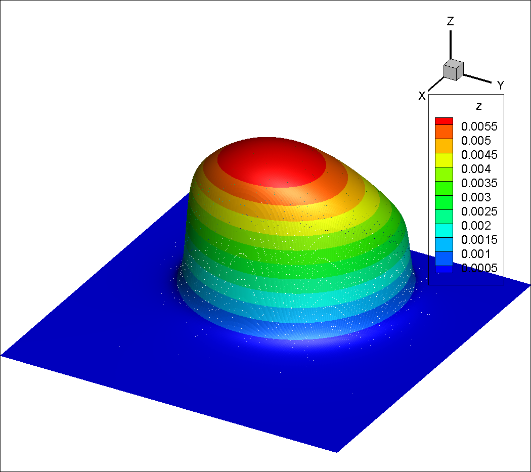
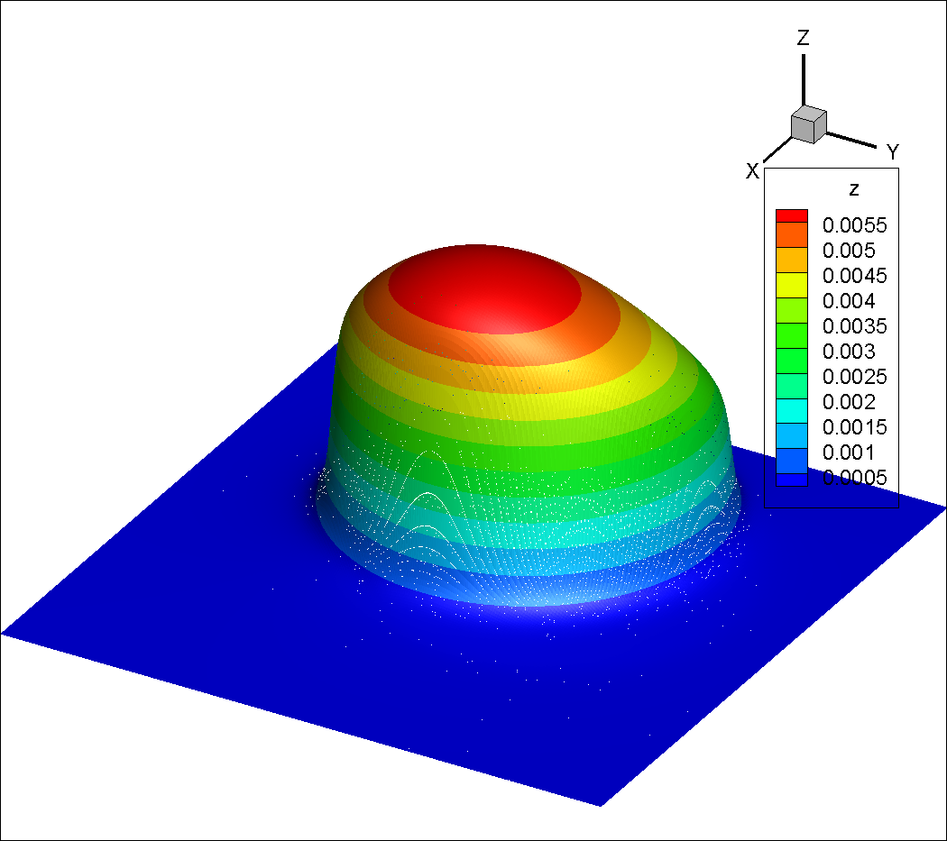
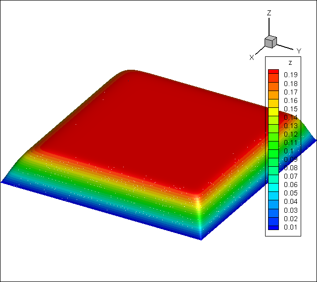
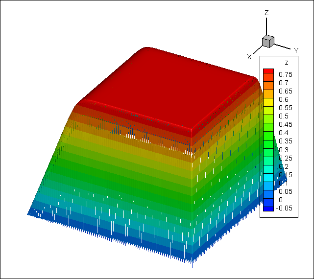
Next, we perform Ensemble HDG computations for the convection dominated case with exact solutions haveing interior layers. But we do not attempt to compute convergence rates here; instead for illustration we plot all the ensemble members at the final time and also plot the exact solution for comparsion. We can see that the Ensemble HDG method is able to capture the very sharp interior layers in the solution with almost no oscillatory behavior, see e.g. Figures 1, 2 and 3.
The domain is and it is uniformly partition into triangles () and also . The initial conditions, boundary conditions, and source terms are chosen to match Equation 1.1 for the data
and the exact solutions are chosen as

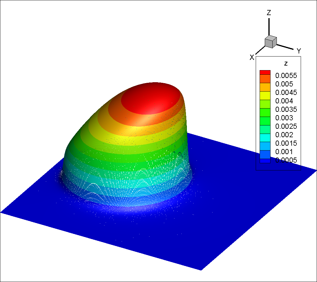

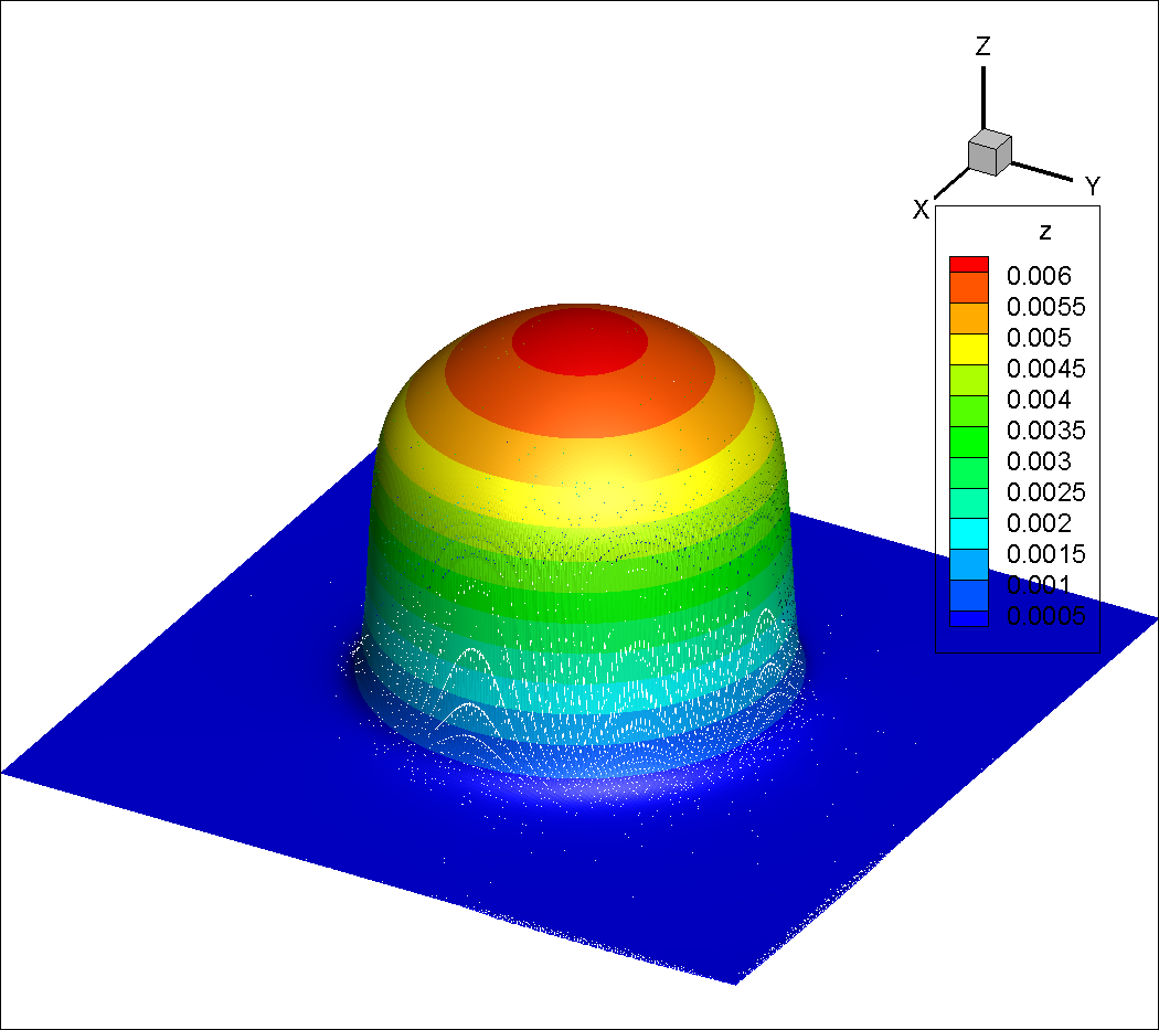
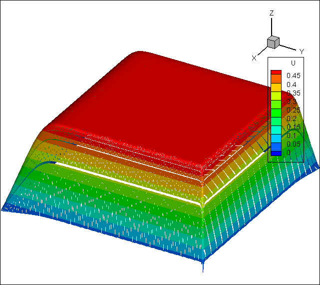
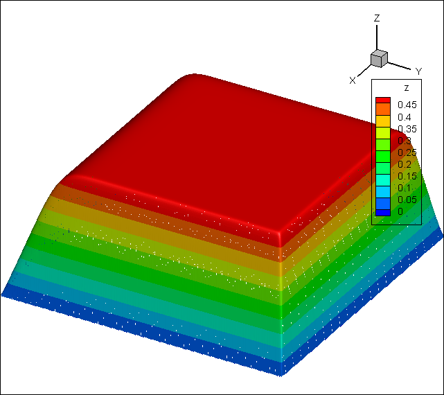
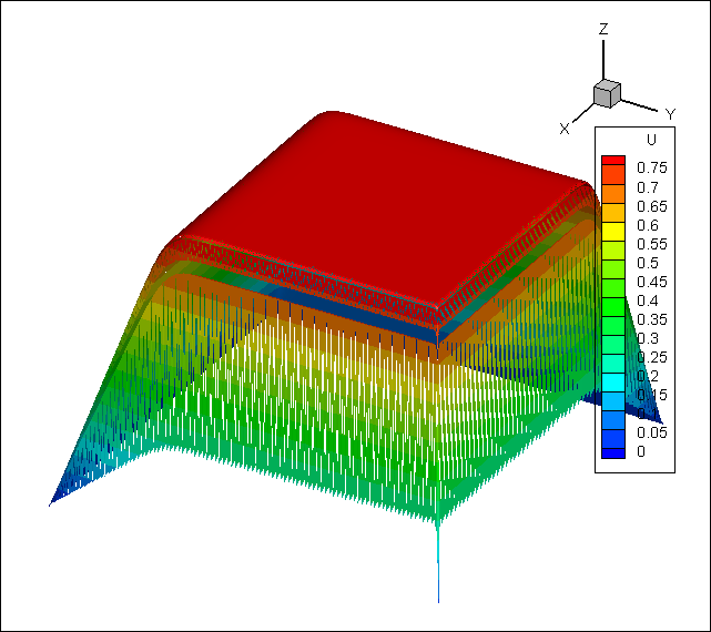
Example 3.
Fianlly, we perform the Ensemble HDG method for a group of convection dominated problems without exact solutions. In this example, the problems exhibit not interior layers but boundary layers. It is well known that the boundary layers are more difficult than interior layers for all numerical methods. Since in Example 2 the Ensemble HDG captured the interior layers without oscillations, we didn’t plot the postprocessed solutions there. However, our numerical test shows that the postprocessed solutions are better than for solutions with boundary layers; see e.g. Figures 4, 5 and 6. We note there is no superconvergent rate even for a single convection dominated diffusion problem PDE using HDG methods, see, e.g. [18].
We plot all the ensemble members and at the final time for comparsion. The domain, the mesh, the time step, the bounday conditions and the initial conditions are the same with Example 2. For the other data, we take

5 Conclusion
In this work, we first devised a superconvergent Ensemble HDG method for parameterized convection diffusion PDEs. This Ensemble HDG method shares one common coefficient matrix and multiple RHS vectors, which is more efficient than performing separate simulations. We proved optimal error estimates for the flux and the scalar variable ; moreover, we obtained the superconvergent rate for . As far as we are aware, this is the first time in the literature.
There are a number of topics that can be explored in the future, including devising high order time stepping methods, a group of convection dominated diffusion PDEs, and stochastic PDEs.
Acknowledgements
G. Chen is supported by China Postdoctoral Science Fou-
ndation grant 2018M633339. G. Chen thanks Missouri University of Science and Technology for hosting him as a visiting scholar; some of this work was completed during his research visit. L. Xu is supported in part by a Key Project of the Major Research Plan of NSFC grant no. 91630205 and the NSFC grant no. 11771068. The authors thank Dr. John Singler for his comments and edits, which significantly improved this paper.
6 Appendix
In this section we only give a proof for (3.12a) and (3.12b), since the rest are similar. To prove (3.12c)-(3.12e), we differentiate the error equations in Lemma 10 with respect to time . It is easy to check that the operators commute with the time derivative, i.e., , since the velocity vector fields are independent of time .
6.1 The equations of the projection of the errors
Lemma 10.
We have the following equalities
| for all . | |||
The proof is similar to the proof of Lemma 4, hence we omit it here.
Lemma 11.
We have the error equations
| (6.2a) | |||
| (6.2b) | |||
for all .
6.2 Estimates for
Lemma 12.
We have
6.3 Dual arguments
The next step is the consideration of the dual problems:
| (6.4) |
Elliptic regularity. To obatin the superconvergent rate, we are going to assume that the domain is such that for any , we have the regularity estimates for these boundary value problems (6.4):
| (6.5) |
It is well known that this holds whenever is a convex polyhedral domain.
Lemma 13.
References
- [1] A. Buffa, T. J. R. Hughes, and G. Sangalli. Analysis of a multiscale discontinuous Galerkin method for convection-diffusion problems. SIAM J. Numer. Anal., 44(4):1420–1440, 2006.
- [2] Aycil Cesmelioglu, Bernardo Cockburn, Ngoc Cuong Nguyen, and Jaume Peraire. Analysis of HDG methods for Oseen equations. J. Sci. Comput., 55(2):392–431, 2013.
- [3] G. Chen, B. Cockburn, J. R. Singler, and Y. Zhang. Superconvergent Interpolatory HDG methods for reaction diffusion equations. Part I: HDG-k methods. In preparation.
- [4] Huangxin Chen, Jingzhi Li, and Weifeng Qiu. Robust a posteriori error estimates for HDG method for convection-diffusion equations. IMA J. Numer. Anal., 36(1):437–462, 2016.
- [5] Yanlai Chen and Bernardo Cockburn. Analysis of variable-degree HDG methods for convection-diffusion equations. Part I: general nonconforming meshes. IMA J. Numer. Anal., 32(4):1267–1293, 2012.
- [6] Yanlai Chen and Bernardo Cockburn. Analysis of variable-degree HDG methods for convection-diffusion equations. Part II: Semimatching nonconforming meshes. Math. Comp., 83(285):87–111, 2014.
- [7] B. Cockburn, N. C. Nguyen, and J. Peraire. HDG methods for hyperbolic problems. In Handbook of numerical methods for hyperbolic problems, volume 17 of Handb. Numer. Anal., pages 173–197. Elsevier/North-Holland, Amsterdam, 2016.
- [8] B. Cockburn, J. R. Singler, and Y. Zhang. Interpolatory HDG Method for Parabolic Semilinear PDEs. Submitted to Journal of Scientific Computing.
- [9] Bernardo Cockburn, Jayadeep Gopalakrishnan, and Raytcho Lazarov. Unified hybridization of discontinuous Galerkin, mixed, and continuous Galerkin methods for second order elliptic problems. SIAM J. Numer. Anal., 47(2):1319–1365, 2009.
- [10] Bernardo Cockburn, Jayadeep Gopalakrishnan, Ngoc Cuong Nguyen, Jaume Peraire, and Francisco-Javier Sayas. Analysis of HDG methods for Stokes flow. Math. Comp., 80(274):723–760, 2011.
- [11] Bernardo Cockburn, Jayadeep Gopalakrishnan, and Francisco-Javier Sayas. A projection-based error analysis of HDG methods. Math. Comp., 79(271):1351–1367, 2010.
- [12] Bernardo Cockburn and Francisco-Javier Sayas. Divergence-conforming HDG methods for Stokes flows. Math. Comp., 83(288):1571–1598, 2014.
- [13] Bernardo Cockburn and Ke Shi. Conditions for superconvergence of HDG methods for Stokes flow. Math. Comp., 82(282):651–671, 2013.
- [14] Bernardo Cockburn and Ke Shi. Devising methods for Stokes flow: an overview. Comput. & Fluids, 98:221–229, 2014.
- [15] Bernardo Cockburn and Chi-Wang Shu. The local discontinuous Galerkin method for time-dependent convection-diffusion systems. SIAM J. Numer. Anal., 35(6):2440–2463, 1998.
- [16] Jim Douglas, Jr. and Todd Dupont. The effect of interpolating the coefficients in nonlinear parabolic Galerkin procedures. Math. Comput., 20(130):360–389, 1975.
- [17] J. A. Fiordilino. A Second Order Ensemble Timestepping Algorithm for Natural Convection. SIAM J. Numer. Anal., 56(2):816–837, 2018.
- [18] Guosheng Fu, Weifeng Qiu, and Wujun Zhang. An analysis of HDG methods for convection-dominated diffusion problems. ESAIM Math. Model. Numer. Anal., 49(1):225–256, 2015.
- [19] M. Gunzburger, N. Jiang, and M. Schneier. A higher-order ensemble/proper orthogonal decomposition method for the nonstationary navier-stokes equations. International Journal of Numerical Analysis and Modeling. to appear.
- [20] M. Gunzburger, N. Jiang, and Z. Wang. An efficient algorithm for simulating ensembles of parameterized flow problems. IMA Journal of Numerical Analysis.
- [21] M. Gunzburger, N. Jiang, and Z. Wang. A second-order time-stepping scheme for simulating ensembles of parameterized flow problems. Comput. Methods Appl. Math. to appear.
- [22] Max Gunzburger, Nan Jiang, and Michael Schneier. An ensemble-proper orthogonal decomposition method for the nonstationary Navier-Stokes equations. SIAM J. Numer. Anal., 55(1):286–304, 2017.
- [23] Nan Jiang. A higher order ensemble simulation algorithm for fluid flows. J. Sci. Comput., 64(1):264–288, 2015.
- [24] Nan Jiang. A second-order ensemble method based on a blended backward differentiation formula timestepping scheme for time-dependent Navier-Stokes equations. Numer. Methods Partial Differential Equations, 33(1):34–61, 2017.
- [25] Nan Jiang and William Layton. An algorithm for fast calculation of flow ensembles. Int. J. Uncertain. Quantif., 4(4):273–301, 2014.
- [26] Nan Jiang and William Layton. Numerical analysis of two ensemble eddy viscosity numerical regularizations of fluid motion. Numer. Methods Partial Differential Equations, 31(3):630–651, 2015.
- [27] Nan Jiang and Hoang Tran. Analysis of a stabilized CNLF method with fast slow wave splittings for flow problems. Comput. Methods Appl. Math., 15(3):307–330, 2015.
- [28] Yan Luo and Zhu Wang. An Ensemble Algorithm for Numerical Solutions to Deterministic and Random Parabolic PDEs. SIAM J. Numer. Anal., 56(2):859–876, 2018.
- [29] Weifeng Qiu and Ke Shi. An HDG method for convection diffusion equation. J. Sci. Comput., 66(1):346–357, 2016.
- [30] Alfio Quarteroni and Alberto Valli. Domain decomposition methods for partial differential equations. Numerical Mathematics and Scientific Computation. The Clarendon Press, Oxford University Press, New York, 1999. Oxford Science Publications.
- [31] Sander Rhebergen and Bernardo Cockburn. A space-time hybridizable discontinuous Galerkin method for incompressible flows on deforming domains. J. Comput. Phys., 231(11):4185–4204, 2012.
- [32] Sander Rhebergen, Bernardo Cockburn, and Jaap J. W. van der Vegt. A space-time discontinuous Galerkin method for the incompressible Navier-Stokes equations. J. Comput. Phys., 233:339–358, 2013.
- [33] M. A. Sánchez, C. Ciuca, N. C. Nguyen, J. Peraire, and B. Cockburn. Symplectic Hamiltonian HDG methods for wave propagation phenomena. J. Comput. Phys., 350:951–973, 2017.
- [34] J. M. Sanz-Serna and L. Abia. Interpolation of the coefficients in nonlinear elliptic Galerkin procedures. SIAM J. Numer. Anal., 21(1):77–83, 1984.
- [35] M. Stanglmeier, N. C. Nguyen, J. Peraire, and B. Cockburn. An explicit hybridizable discontinuous Galerkin method for the acoustic wave equation. Comput. Methods Appl. Mech. Engrg., 300:748–769, 2016.
- [36] Aziz Takhirov, Monika Neda, and Jiajia Waters. Time relaxation algorithm for flow ensembles. Numer. Methods Partial Differential Equations, 32(3):757–777, 2016.
- [37] Jan Česenek and Miloslav Feistauer. Theory of the space-time discontinuous Galerkin method for nonstationary parabolic problems with nonlinear convection and diffusion. SIAM J. Numer. Anal., 50(3):1181–1206, 2012.
- [38] Jinchao Xu. Iterative methods by space decomposition and subspace correction. SIAM Rev., 34(4):581–613, 1992.