Optimal Collusion-Free Teaching

Abstract

Formal models of learning from teachers need to respect certain criteria to avoid collusion. The most commonly accepted notion of collusion-freeness was proposed by Goldman and Mathias (1996), and various teaching models obeying their criterion have been studied. For each model $M$ and each concept class ${\mathcal{C}}$, a parameter $M$-$\mathrm{TD}({\mathcal{C}})$ refers to the teaching dimension of concept class ${\mathcal{C}}$ in model $M$—defined to be the number of examples required for teaching a concept, in the worst case over all concepts in ${\mathcal{C}}$.

This paper introduces a new model of teaching, called no-clash teaching, together with the corresponding parameter $\mathrm{NCTD}({\mathcal{C}})$. No-clash teaching is provably optimal in the strong sense that, given any concept class ${\mathcal{C}}$ and any model $M$ obeying Goldman and Mathias’s collusion-freeness criterion, one obtains $\mathrm{NCTD}({\mathcal{C}})\leq M$-$\mathrm{TD}({\mathcal{C}})$. We also study a corresponding notion $\mathrm{NCTD}^{+}$ for the case of learning from positive data only, establish useful bounds on $\mathrm{NCTD}$ and $\mathrm{NCTD}^{+}$, and discuss relations of these parameters to the VC-dimension and to sample compression.

In addition to formulating an optimal model of collusion-free teaching, our main results are on the computational complexity of deciding whether $\mathrm{NCTD}^{+}({\mathcal{C}})=k$ (or $\mathrm{NCTD}({\mathcal{C}})=k$) for given ${\mathcal{C}}$ and $k$. We show some such decision problems to be equivalent to the existence question for certain constrained matchings in bipartite graphs. Our NP-hardness results for the latter are of independent interest in the study of constrained graph matchings.

Keywords: machine teaching, constrained graph matchings, sample compression

1 Introduction

Models of machine learning from carefully chosen examples, i.e., from teachers, have gained increased interest in recent years, due to various application areas, such as robotics (Argall et al., 2009), trustworthy AI (Zhu et al., 2018), and pedagogy (Shafto et al., 2014). Machine teaching is also related to inverse reinforcement learning (Ho et al., 2016), to sample compression (Moran et al., 2015; Doliwa et al., 2014), and to curriculum learning (Bengio et al., 2009). The paper at hand is concerned with abstract notions of teaching, as studied in computational learning theory.

A variety of formal models of teaching have been proposed in the literature, for example, the classical teaching dimension model (Goldman and Kearns, 1995), the optimal teacher model (Balbach, 2008), recursive teaching (Zilles et al., 2011), or preference-based teaching (Gao et al., 2017).

In each of these models, a mapping $T$ (the teacher) assigns a finite set $T(C)$ of correctly labelled examples to a concept $C$ in a concept class $\mathcal{C}$ in a way that the learner can reconstruct $C$ from $T(C)$. Intuitively, unfair collusion between the teacher and the learner should not be allowed in any formal model of teaching. For example, one would not want the teacher and learner to agree on a total order over the domain and a total order over the concept class and then to simply use the $i$th instance in the domain for teaching the $i$th concept, irrespective of the actual structure of the concept class.

However, there is no general definition of what constitutes collusion, and of what constitutes desirable or undesirable forms of learning. In this manuscript, we focus on a notion of collusion that was proposed by Goldman and Mathias (1996) and that has been adopted by the majority of teaching models studied in the literature. In a nutshell, Goldman and Mathias’s model demands that, (i) the examples in $T(C)$ are labelled consistently with $C$, and (ii) if the learner correctly identifies $C$ from $T(C)$, then it will also identify $C$ from any superset $S$ of $T(C)$ as long as the sample set $S$ remains consistent with $C$. In other words, adding more information about $C$ to $T(C)$ will not divert the learner to an incorrect hypothesis.

Most existing abstract models of machine teaching are collusion-free in this sense. Historically, some of these models were designed in order to overcome weaknesses of the previous models. For example, the optimal teacher model by Balbach (2008) is designed to overcome limitations of the classical teaching dimension model, and was likewise superseded by the recursive teaching model (Zilles et al., 2011). The latter again was inapplicable to many interesting infinite concept classes, which gave rise to the model of preference-based teaching (Gao et al., 2017). Each model strictly dominates the previous one in terms of the teaching complexity, i.e., the worst-case number of examples needed for teaching a concept in the underlying concept class ${\mathcal{C}}$. In this context, one quite natural question has been ignored in the literature to date: what is the smallest teaching complexity that can be achieved under Goldman and Mathias’s condition of collusion-freeness? This is exactly the question addressed in this paper.

Our first contribution is the formal definition of a collusion-free teaching model that has, for every concept class ${\mathcal{C}}$, the provably smallest teaching complexity among all collusion-free teaching models. We call this model no-clash teaching, since its core property, which turns out to be characteristic for collusion-freeness, requires that no pair of concepts are consistent with the union of their teaching sets. A similar property was used once in the literature in the context of sample compression schemes (Kuzmin and Warmuth, 2007), and dubbed the non-clashing property.

For example, consider a concept class (i.e., set system) ${\mathcal{C}}$ over the instance space $\{1,2,3,4\}$, consisting of the four concepts of the form $\{i,(i+1)\bmod 4\}$ for $1\leq i\leq 4$. Then no-clash teaching is possible by assigning the singleton set $\{(i,1)\}$ (interpreted as the information “$i$ belongs to the target concept”) as a teaching set to the concept $\{i,(i+1)\bmod 4\}$; no two distinct concepts are consistent with the union of their assigned teaching sets. Thus, in the no-clash setting, each concept in ${\mathcal{C}}$ can be taught with a single example. By comparison, consider the classical teaching dimension model, in which a teaching set for a given concept is required to be inconsistent with all other concepts in the concept class (Goldman and Kearns, 1995). It is not hard to see that, under such constraints, no concept in ${\mathcal{C}}$ can be taught with a single example; a smallest teaching set for concept $\{i,(i+1)\bmod 4\}$ would then be $\{(i,1),((i+1)\bmod 4,1)\}$.

We call the worst-case number of examples needed for non-clashing teaching of any concept $C$ in a given concept class ${\mathcal{C}}$ the no-clash teaching dimension of ${\mathcal{C}}$, abbreviated $\mathrm{NCTD}({\mathcal{C}})$, and we study a variant $\mathrm{NCTD}^{+}({\mathcal{C}})$ in which teaching uses only positive examples. In the example above, $\mathrm{NCTD}=\mathrm{NCTD}^{+}=1$, while the classical teaching dimension is $2$.

The value $\mathrm{NCTD}({\mathcal{C}})$ being the smallest collusion-free teaching complexity parameter of ${\mathcal{C}}$ makes it interesting for several reasons.

(1) $\mathrm{NCTD}$ represents the limit of data efficiency in teaching when obeying Goldman and Mathias’s notion of collusion-freeness. Therefore the study of $\mathrm{NCTD}$ has the potential to further our understanding how collusion-freeness constrains teaching. It will also help to compare other notions of collusion-freeness (see, e.g., (Zilles et al., 2011)) to that of Goldman and Mathias.

(2) An open question in computational learning theory is whether the VC-dimension ($\mathrm{VCD}$), (Vapnik and Chervonenkis, 1971), which characterizes the sample complexity of learning from randomly chosen examples, also characterizes teaching complexity for some reasonable notion of teaching. Recently, the first strong connections between teaching and $\mathrm{VCD}$ were established, culminating in an upper bound on the recursive teaching dimension ($\mathrm{RTD}$) that is quadratic in $\mathrm{VCD}$ (Hu et al., 2017), but it remains open whether this bound can be improved to be linear in $\mathrm{VCD}$. Obviously, now $\mathrm{NCTD}$ is a much stronger candidate for a linear relationship with $\mathrm{VCD}$ than $\mathrm{RTD}$ is. In fact, there is no concept class known yet for which $\mathrm{NCTD}$ exceeds $\mathrm{VCD}$.

(3) The problem of relating teaching complexity to $\mathrm{VCD}$ is connected to the famous open problem of determining whether $\mathrm{VCD}$ is an upper bound on the size of the smallest possible sample compression scheme (Littlestone and Warmuth, 1986; Floyd and Warmuth, 1995) of a concept class. Some interesting relations between sample compression and teaching have been established for $\mathrm{RTD}$ (Moran et al., 2015; Doliwa et al., 2014; Darnstädt et al., 2016). The study of $\mathrm{NCTD}$ can potentially strengthen such relations.

In addition, an important contribution of our paper is to link $\mathrm{NCTD}$ to the extensively developed theory of constrained graph matching. We show that the question whether $\mathrm{NCTD}^{+}=1$ is equivalent to a very natural constrained bipartite matching problem which has apparently not yet been studied in the literature. We proceed by proving that this particular matching problem is NP-hard—a result that generalizes to larger values of $\mathrm{NCTD}^{+}$ as well as to $\mathrm{NCTD}$. By comparison, the question whether $\mathrm{RTD}^{+}=1$ or $\mathrm{RTD}=1$ can be answered in linear time.

To sum up, our new notion of optimal collusion-free teaching is of relevance to the study of important open problems in computational learning theory as well as of fundamental graph-theoretic decision problems, and therefore appears to be worth studying in more detail.

2 Preliminaries

Given a domain ${\mathcal{X}}$, a concept over ${\mathcal{X}}$ is a subset $C\subseteq{\mathcal{X}}$, and we usually denote by ${\mathcal{C}}$ a concept class over ${\mathcal{X}}$, i.e., a set of concepts over ${\mathcal{X}}$. Implicitly, we identify a concept $C$ over ${\mathcal{X}}$ with a mapping $C:{\mathcal{X}}\rightarrow\{0,1\}$, where $C(x)=1$ iff $x\in C$. By $\mbox{$\mathrm{VCD}$}({\mathcal{C}})$, we denote the VC-dimension of ${\mathcal{C}}$.

A labelled example is a pair $(x,\ell)\in{\mathcal{X}}\times\{0,1\}$, and it is consistent with a concept $C$ if $C(x)=\ell$. Likewise, a set $S$ of labelled examples over ${\mathcal{X}}$, which is also called a sample set, is consistent with $C$, if every element of $S$ is consistent with $C$. An example with the label $\ell=1$ is a positive example, while $\ell=0$ is the label of a negative example.

Intuitively, the notion of teaching refers to compressing any concept in a given concept class to a consistent sample set.

Definition 1

Let ${\mathcal{C}}$ be a concept class over a domain ${\mathcal{X}}$. A teacher mapping for ${\mathcal{C}}$ is a mapping $T$ on ${\mathcal{C}}$ such that, for all $C\in{\mathcal{C}}$, $T(C)$ is a finite sample set $S\subseteq{\mathcal{X}}\times\{0,1\}$ that is consistent with $C$.

The first model of teaching that was proposed in the literature required from a teacher mapping $T$ that the concept $C\in{\mathcal{C}}$ be the only concept in ${\mathcal{C}}$ that is consistent with $T(C)$, for any $C\in{\mathcal{C}}$ (Shinohara and Miyano, 1991; Goldman and Kearns, 1995). This led to the definition of the well-known teaching dimension parameter.

Definition 2 (Shinohara and Miyano (1991); Goldman and Kearns (1995))

Let ${\mathcal{C}}$ be a concept class over a domain ${\mathcal{X}}$ and $C\in{\mathcal{C}}$ be a concept. A teaching set for $C$ (with respect to ${\mathcal{C}}$) is a sample set $S$ such that $C$ is the only concept in ${\mathcal{C}}$ consistent with $S$. The teaching dimension of $C$ in ${\mathcal{C}}$, denoted by $\mathrm{TD}(C,{\mathcal{C}})$, is the size of the smallest teaching set for $C$ with respect to ${\mathcal{C}}$. The teaching dimension of ${\mathcal{C}}$ is then defined as $\mathrm{TD}({\mathcal{C}})=\sup\{\mathrm{TD}(C,{\mathcal{C}})\mid C\in{\mathcal{C}}\}$.

For example, let ${\mathcal{C}}$ be a concept class over a domain ${\mathcal{X}}$ of exactly $m$ elements, containing the empty concept, all singleton concepts over ${\mathcal{X}}$, and no other concepts. Then $\mathrm{TD}(\{x\},{\mathcal{C}})=1$ for each singleton concept $\{x\}$, since $\{(x,1)\}$ serves as a teaching set for $\{x\}$. By comparison, $\mathrm{TD}(\emptyset,{\mathcal{C}})=m$, since any set of up to $m-1$ negative examples is consistent with some singleton concept, so that all $m$ negative examples need to be presented in order to identify the empty concept. Consequently, $\mathrm{TD}({\mathcal{C}})=\sup\{\mathrm{TD}(C,{\mathcal{C}})\mid C\in{\mathcal{C}}\}=m$.

As mentioned in the introduction, various notions of teaching have been proposed in the literature. The one that is most relevant to our work is the model of preference-based teaching. In this model, intuitively, a preference relation on ${\mathcal{C}}$ is used to reduce the size of teaching sets. In particular, a concept $C$ need no longer be the only concept consistent with its teaching set $T(C)$; it suffices if $C$ is the unique most preferred concept in ${\mathcal{C}}$ that is consistent with ${\mathcal{C}}$. In order to avoid cyclic preferences, the preference relation is required to form a partial order over ${\mathcal{C}}$.

Definition 3 (Gao et al. (2017))

Let ${\mathcal{C}}$ be a concept class over a domain ${\mathcal{X}}$ and $\succ$ any binary relation that forms a strict (possibly non-total) order over ${\mathcal{C}}$. We say that concept $C$ is preferred over concept $C^{\prime}$ (with respect to $\succ$), if $C\succ C^{\prime}$. The preference-based teaching dimension of $C$ with respect to ${\mathcal{C}}$ and $\succ$, denoted by $\mathrm{PBTD}(C,{\mathcal{C}},\succ)$, is the size of the smallest sample set $S$ such that

1. $S$ is consistent with $C$, and

2. $C\succ C^{\prime}$ for all $C^{\prime}\in{\mathcal{C}}\setminus\{C\}$ such that $S$ is consistent with $C^{\prime}$.

We write $\mathrm{PBTD}({\mathcal{C}},\succ)=\sup\{\mathrm{PBTD}(C,{\mathcal{C}},\succ)\mid C\in{\mathcal{C}}\}$. Finally, the preference-based teaching dimension of ${\mathcal{C}}$, denoted by $\mathrm{PBTD}({\mathcal{C}})$, is defined by

$$\mathrm{PBTD}({\mathcal{C}})=\min\{\mathrm{PBTD}({\mathcal{C}},\succ)\mid\,\succ\subseteq{\mathcal{C}}\times{\mathcal{C}}\mbox{ and }\succ\mbox{ forms a strict order on }{\mathcal{C}}\}\,.$$

An interesting variant of preference-based teaching is obtained when disallowing negative examples in teaching. Learning from positive examples only has been studied extensively in the computational learning theory literature, see, e.g., (Denis, 2001; Angluin, 1980) and is motivated by studies on language acquisition (Wexler and Culicover, 1980) or, more recently, by problems of learning user preferences from a user’s interactions with, say, an e-commerce system (Schwab et al., 2000), as well as by problems in bioinformatics (Wang et al., 2006).

Definition 4 (Gao et al. (2017))

Let ${\mathcal{C}}$ be a concept class over a domain ${\mathcal{X}}$. The positive preference-based teaching dimension of ${\mathcal{C}}$, denoted by $\mathrm{PBTD}^{+}({\mathcal{C}})$, is defined analogously to $\mathrm{PBTD}({\mathcal{C}})$, where the sets $S$ in Definition 3 are required to contain only positive examples.

In the same way, one can define the notion $\mathrm{TD}^{+}$. The following property, proven by Gao et al. (2017), is crucial when computing the $\mathrm{PBTD}$ and $\mathrm{PBTD}^{+}$ of finite classes.

Proposition 5 (Gao et al. (2017))

Let ${\mathcal{C}}$ be a finite concept class. If $\mathrm{PBTD}({\mathcal{C}})\!=\!d$, then ${\mathcal{C}}$ contains some $C$ with $\mathrm{TD}(C,{\mathcal{C}})\leq d$. If $\mathrm{PBTD}^{+}({\mathcal{C}})\!=\!d$, then ${\mathcal{C}}$ contains some $C$ with $\mathrm{TD}^{+}(C,{\mathcal{C}})\leq d$.

This result immediately implies that $\mathrm{PBTD}$ and the well-known notion of $\mathrm{RTD}$ coincide for finite concepts classes, and so do $\mathrm{PBTD}^{+}$ and $\mathrm{RTD}^{+}$.

3 Collusion-free Teaching and the Non-Clashing Property

While there is no objective measure of how “reasonable” a formal model of teaching is, the literature offers some notions of what constitutes an “acceptable” model of teaching, i.e., one in which the teacher and learner do not collude. So far, the notion of collusion-free teaching that found the most positive resonance in the literature is the one defined by Goldman and Mathias.

Definition 6 (Goldman and Mathias (1996))

Let ${\mathcal{C}}$ be a concept class over ${\mathcal{X}}$ and $T$ a teacher mapping on ${\mathcal{C}}$. Let $L$ be a learner mapping that assigns to each set of labelled examples a concept over ${\mathcal{X}}$. The pair $(T,L)$ is successful on ${\mathcal{C}}$ if $L(T(C))=C$ for all $C\in{\mathcal{C}}$. The pair $(T,L)$ is collusion-free on ${\mathcal{C}}$ if $L(S)=L(T(C))$ for any $C\in{\mathcal{C}}$ and any set $S$ of labelled examples such that $S$ is consistent with $C$ and $S$ contains $T(C)$.

Intuitively, Goldman and Mathias’s definition captures the idea that a learner conjecturing concept $C$ will not change its mind when given additional information consistent with $C$.

For example, teacher-learner pairs following the classical teaching dimension model, Balbach’s optimal teacher model, the recursive teaching model, or the preference-based teaching model are always collusion-free according to Definition 6. Of these models, the classical teaching dimension model is the one imposing the most constraints on the mapping $T$, followed by Balbach’s optimal teaching, recursive teaching, and preference-based teaching in that order. Consequently, the “teaching complexity” among these models is lowest for preference-based teaching; if every concept in a concept class ${\mathcal{C}}$ can be taught with at most $z$ examples in any of these models, then every concept in ${\mathcal{C}}$ can be taught with at most $z$ examples in the preference-based model.

One can still argue that the preference-based model is unnecessarily constraining. Preference-based teaching of a concept class ${\mathcal{C}}$ relies on a preference relation that induces a strict order on ${\mathcal{C}}$. However, this strict order is used by the learner only after the teaching set has been communicated, since the learner chooses the unique most preferred concept among those consistent with the set of examples provided by the teacher. One might consider loosening the constraints by, for example, demanding only that the set of concepts consistent with any chosen teaching set be ordered under the chosen preference relation (rather than requiring acyclic preferences over the whole concept class). In the same vein, one could relax more conditions—every relaxation might result in a more powerful model of teaching satisfying the collusion-free property.

In this manuscript, we will define the provably most powerful model of teaching that is collusion-free in the sense proposed by Goldman and Mathias (1996), namely a model that adheres to no other constraints on the teacher-learner pairs $(T,L)$ than those given by Goldman and Mathias: (i) $T$ is a teacher mapping; (ii) $(T,L)$ is successful on ${\mathcal{C}}$; and (iii) $(T,L)$ is collusion-free on ${\mathcal{C}}$.

Before we define this model formally, we introduce a crucial property that was originally proposed by Kuzmin and Warmuth (2007) in the context of unlabeled sample compression.

Definition 7

Let ${\mathcal{C}}$ be a concept class and $T$ be a teacher mapping on ${\mathcal{C}}$. We say that $T$ is non-clashing (on ${\mathcal{C}}$) if and only if there are no two distinct $C,C^{\prime}\in{\mathcal{C}}$ such that both $T(C)$ is consistent with $C^{\prime}$ and $T(C^{\prime})$ is consistent with $C$.

It turns out that, for a teacher mapping $T$, the non-clashing property is equivalent to the existence of a learner mapping $L$ such that $(T,L)$ is successful and collusion-free:

Theorem 8

Let ${\mathcal{C}}$ be a concept class over the instance space ${\mathcal{X}}$. Let $T$ be a teacher mapping on ${\mathcal{C}}$. Then the following two conditions are equivalent:

1. $T$ is non-clashing on ${\mathcal{C}}$.

2. There is a mapping $L:2^{{\mathcal{X}}\times\{0,1\}}\rightarrow{\mathcal{C}}$ such that $(T,L)$ is both successful and collusion-free on ${\mathcal{C}}$.

Proof  First, suppose $T$ is a non-clashing teacher mapping, and define $L$ as follows. Given any set $S$ of labelled examples as input, $L$ checks for the existence of a concept $C\in{\mathcal{C}}$ such that $T(C)\subseteq S$ and $C$ is consistent with $S$. If such a concept $C$ is found, $L$ returns an arbitrary such $C$; otherwise $L$ returns some default concept in ${\mathcal{C}}$.

To show that $(T,L)$ is successful and collusion-free, suppose there is some concept $C\in{\mathcal{C}}$ such that a given set $S$ of labelled examples is consistent with $C$ and contains $T(C)$. We claim that then such $C$ is uniquely determined. For if there were two distinct concepts $C,C^{\prime}\in{\mathcal{C}}$ consistent with $S$ such that $T(C)\cup T(C^{\prime})\subseteq S$, then $T(C^{\prime})$, being a subset of $S$, would be consistent with $C$ and, likewise, $T(C)$ would be consistent with $C^{\prime}$—in contradiction to the non-clashing property of $T$. From the definition of $L$, it then follows that $(T,L)$ is successful and collusion-free.

Second, suppose $T$ is a teacher mapping and there is a mapping $L$ such that $(T,L)$ is successful and collusion-free, i.e., for all $C\in{\mathcal{C}}$, we have $L(S)=L(T(C))=C$ whenever $S$ is consistent with $C$ and contains $T(C)$. To see that $T$ is non-clashing, suppose two concepts $C,C^{\prime}\in{\mathcal{C}}$ are both consistent with $T(C)\cup T(C^{\prime})$. Then $C=L(T(C))=L(T(C)\cup T(C^{\prime}))=L(T(C^{\prime}))=C^{\prime}$.  

Consequently, teaching with non-clashing teacher mappings is, in terms of the worst-case number of examples required, the most efficient model that obeys Goldman and Mathias’s notion of collusion-freeness. We hence define the notion of no-clash teaching dimension as follows.

Definition 9

Let ${\mathcal{C}}$ be a concept class over the instance space ${\mathcal{X}}$. Let $T:{\mathcal{C}}\rightarrow({\mathcal{X}}\times\{0,1\})^{*}$ be a non-clashing teacher mapping. The order of $T$ on ${\mathcal{C}}$, denoted by $\mathrm{ord}(T,{\mathcal{C}})$, is then defined by $\mathrm{ord}(T,{\mathcal{C}})=\sup\{|T(C)|\mid C\in{\mathcal{C}}\}$. The No-Clash Teaching Dimension of ${\mathcal{C}}$, denoted by $\mathrm{NCTD}({\mathcal{C}})$, is defined as $\mathrm{NCTD}({\mathcal{C}})=\min\{\mathrm{ord}(T,{\mathcal{C}})\mid T\mbox{ is a non-clashing teacher mapping for }{\mathcal{C}}\}$.

From Theorem 8 we obtain that, for every concept class ${\mathcal{C}}$,

$$\mathrm{NCTD}({\mathcal{C}})=\min\{\mathrm{ord}(T,{\mathcal{C}})\mid\mbox{ there exists an }L\mbox{ s.t. }(T,L)\mbox{ is successful and collusion-free on }{\mathcal{C}}\}.$$

As in the case of preference-based teaching, it is natural to study a variant of non-clashing teaching that uses positive examples only.

Definition 10

Let ${\mathcal{C}}$ be a concept class over the domain ${\mathcal{X}}$. A teacher mapping $T$ is called positive on ${\mathcal{C}}$ if $T(C)\subseteq{\mathcal{X}}\times\{1\}$ for all $C\in{\mathcal{C}}$. We then define $\mathrm{NCTD}^{+}({\mathcal{C}})=\min\{\mathrm{ord}(T,{\mathcal{C}})\mid T\mbox{ is a positive non-clashing teacher mapping for }{\mathcal{C}}\}$.

Furthermore, for finite domains ${\mathcal{X}}$, it will be helpful to have the notion of average no-clash teaching dimension:

Definition 11

Let ${\mathcal{C}}$ be a concept class over the finite domain ${\mathcal{X}}$. The Average No-Clash Teaching Dimension of ${\mathcal{C}}$, denoted by $\mathrm{ANCTD}({\mathcal{C}})$, is defined as

$$\mathrm{ANCTD}({\mathcal{C}})=\min\left\{\left.\frac{1}{|{\mathcal{C}}|}\sum_{C\in{\mathcal{C}}}|T(C)|\right|\mbox{ $T$ is a non-clashing teacher mapping for ${\mathcal{C}}$}\right\}\enspace.$$

Remark 12

It follows immediately from the pigeon-hole principle that $\mathrm{NCTD}({\mathcal{C}})\geq\lceil\mathrm{ANCTD}({\mathcal{C}})\rceil$.

In the following we describe a natural normal form for non-clashing teacher mappings. $T^{\prime}$ is said to be an extension of $T$ if $T(C)\subseteq T^{\prime}(C)$ holds for every $C\in{\mathcal{C}}$. Clearly, if $T^{\prime}$ is an extension of $T$ and $T$ is non-clashing, then $T^{\prime}$ is non-clashing.

Proposition 13

(a) Let $T$ be a non-clashing teacher mapping for ${\mathcal{C}}$. Then there is a non-clashing teacher mapping $T^{\prime}$ for ${\mathcal{C}}$ such that $|T^{\prime}(C)|=\mathrm{ord}(T,{\mathcal{C}})$ for all $C\in{\mathcal{C}}$.
(b) Let $T$ be a positive non-clashing teacher mapping for ${\mathcal{C}}$. Then there is a positive non-clashing teacher mapping $T^{\prime}$ for ${\mathcal{C}}$ such that $|T^{\prime}(C)|=\min\{|C|,\mathrm{ord}(T,{\mathcal{C}})\}$ for all $C\in{\mathcal{C}}$.

While many of our definitions and results apply to both finite and infinite concept classes, except where explicitly stated otherwise, we will hereafter assume that ${\mathcal{X}}$ (and ${\mathcal{C}}$) are finite.

4 Lower Bounds on $\mathrm{NCTD}$ and $\mathrm{NCTD}^{+}$

To establish lower bounds on $\mathrm{NCTD}$ and $\mathrm{NCTD}^{+}$ for finite concept classes, we first show that $\mathrm{NCTD}({\mathcal{C}})$ must be at least as large as the smallest $d$ satisfying $|{\mathcal{C}}|\leq 2^{d}{|{\mathcal{X}}|\choose d}$. A similar statement then follows for $\mathrm{NCTD}^{+}$. In fact, we prove a slightly stronger result, replacing $|{\mathcal{X}}|$ with a potentially smaller value:

Definition 14

We define ${\mathcal{X}}_{T}\subseteq{\mathcal{X}}$ as the set of instances that are part of a labelled example in a teaching set $T(C)$ for some $C\in{\mathcal{C}}$. Moreover, we define

$$X({\mathcal{C}})=\min\{|{\mathcal{X}}_{T}|:\ \mbox{$T$ is a non-clashing teacher mapping for ${\mathcal{C}}$ with }\mathrm{ord}({\mathcal{C}},T)=\mathrm{NCTD}({\mathcal{C}})\}\enspace.$$

Intuitively, $X({\mathcal{C}})$ is the smallest number of instances that must be employed by any optimal non-clashing teacher mapping for ${\mathcal{C}}$. Likewise, we define $X^{+}({\mathcal{C}})$ for positive non-clashing teaching.

Theorem 15

Let ${\mathcal{C}}$ be any concept class.

1. If $\mathrm{NCTD}({\mathcal{C}})=d$, then $|{\mathcal{C}}|\leq 2^{d}{X({\mathcal{C}})\choose d}$.

2. If $\mathrm{NCTD}^{+}({\mathcal{C}})=d$, then $|{\mathcal{C}}|\leq\sum_{i=0}^{d}{X^{+}({\mathcal{C}})\choose i}$.

Proof  To prove statement 1, let ${\mathcal{X}}^{\prime}$ be a subset of size $X({\mathcal{C}})$ of ${\mathcal{X}}$. Let $C\mapsto T(C)\subseteq{\mathcal{X}}^{\prime}\times\{0,1\}$ be a consistent and non-clashing mapping which witnesses that $\mathrm{NCTD}({\mathcal{C}})=d$, and let $L$ be the mapping such that $L(T(C))=C$ for all $C\in{\mathcal{C}}$. By Proposition 13, one may assume without loss of generality that $|T(C)|=d$ for all $C\in{\mathcal{C}}$. Since $T$ is an injective mapping and there are only $2^{d}{X({\mathcal{C}})\choose d}$ labelled teaching sets at our disposal, the claim follows.

Statement 2 is proven analogously, taking into consideration that, in the $\mathrm{NCTD}^{+}$ case, we do not have an analogous statement to Proposition 13, since a concept does not in general contain $d$ or more elements. Note that the formula has no factors $2^{i}$ since there are no options for labelling the instances in any set $T(C)$.  

We will next establish a useful lower bound on $\mathrm{NCTD}({\mathcal{C}})$, as well as as a related lower bound on $\mathrm{NCTD}^{+}({\mathcal{C}})$, based on the number of neighbors of any concept in ${\mathcal{C}}$.

A concept $C^{\prime}\in{\mathcal{C}}$ is a neighbor of concept $C\in{\mathcal{C}}$ if it differs from $C$ on exactly one instance, i.e., if the symmetric difference $C\Delta C^{\prime}:=(C\setminus C^{\prime})\cup(C^{\prime}\setminus C)$ has size one. The degree of $C\in{\mathcal{C}}$, denoted as $\deg_{\mathcal{C}}(C)$, is defined as the number of neighbors of $C$ in ${\mathcal{C}}$. The average degree of concepts in ${\mathcal{C}}$ is then denoted by

$$\deg_{avg}({\mathcal{C}}):=\frac{1}{|{\mathcal{C}}|}\cdot\sum_{C\in{\mathcal{C}}}\deg_{\mathcal{C}}(C)\,.$$

The dominance of $C\in{\mathcal{C}}$, denoted as $\mathrm{dom}_{\mathcal{C}}(C)$, is defined as the number of smaller neighbors of $C$ in ${\mathcal{C}}$, i.e. neighbors that contain exactly one fewer instance than $C$.

Theorem 16

Every concept class ${\mathcal{C}}$ over a finite domain satisfies (i) $\mathrm{ANCTD}({\mathcal{C}})\geq\frac{1}{2}\cdot\deg_{avg}({\mathcal{C}})$
and (ii) $\mathrm{NCTD}({\mathcal{C}})\geq\lceil\frac{1}{2}\cdot\deg_{avg}({\mathcal{C}})\rceil$.

Proof  For assertion (i), let $T$ be any non-clashing teacher mapping for ${\mathcal{C}}$. If $C_{1}$ and $C_{2}$ are neighbors, say $C_{1}\Delta C_{2}=\{x_{i}\}$, then at least one of the sets $T(C_{1}),T(C_{2})$ must contain $x_{i}$. We obtain $\sum_{C\in{\mathcal{C}}}|T(C)|\geq\frac{1}{2}\cdot\sum_{C\in{\mathcal{C}}}\deg_{\mathcal{C}}(C)=|{\mathcal{C}}|\cdot\frac{1}{2}\cdot\deg_{avg}({\mathcal{C}})$. Assertion (ii) is immediate from (i), by Remark 12.  

Theorem 17

Every concept class ${\mathcal{C}}$ over a finite domain satisfies $\mathrm{NCTD}^{+}({\mathcal{C}})\geq\max_{C\in{\mathcal{C}}}\mathrm{dom}_{\mathcal{C}}(C)$.

Proof  If the smaller neighbor $C^{\prime}$ of $C\in{\mathcal{C}}$ differs from $C$ on instance $x_{i}$, then $(x_{i},1)$ must be used in teaching $C$. Hence, every $C\in{\mathcal{C}}$ must have a positive teaching set of size at least $\mathrm{dom}_{\mathcal{C}}(C)$.  

Although the lower bounds in Theorems 16 and 17 are not expected to be attained very often, the following Remark shows that they are sometimes tight:

Remark 18

Let ${\mathcal{P}}_{m}$ be the powerset over the domain $\{x_{1},\ldots,x_{m}\}$. Since every concept in ${\mathcal{P}}_{m}$ has degree $m$, clearly $\deg_{avg}({\mathcal{P}}_{2})=m$. It follows from Theorem 16 that $\mathrm{ANCTD}({\mathcal{P}}_{m})\geq m/2$ and hence $\mathrm{NCTD}({\mathcal{P}}_{m})\geq\lceil m/2\rceil$. Furthermore, since $\mathrm{dom}_{{\mathcal{P}}_{m}}(\{x_{1},\ldots,x_{m}\})=m$, it follows from Theorem 17 that $\mathrm{NCTD}^{+}({\mathcal{P}}_{m})\geq m$. But the positive mapping $T$ that maps $S\in{\mathcal{P}}_{m}$ to $S\times\{1\}$ is trivially non-clashing, and hence $\mathrm{NCTD}^{+}({\mathcal{P}}_{m})=m$ and $\mathrm{ANCTD}({\mathcal{P}}_{m})=m/2$. As the mapping $T$ given by

$$\emptyset\mapsto\{(a,0)\},\{a\}\mapsto\{(b,0)\},\{b\}\mapsto\{(b,1)\},\{a,b\}\mapsto\{(a,1)\}\enspace,$$

is non-clashing for ${\mathcal{P}}_{2}$, it follows that $\mathrm{NCTD}({\mathcal{P}}_{2})=1$. As we shall see in Theorem 23, this generalizes to $\mathrm{NCTD}({\mathcal{P}}_{m})=\lceil m/2\rceil$.

We note that the maximum degree of a concept in ${\mathcal{C}}$ is in general not an upper bound on $\mathrm{NCTD}({\mathcal{C}})$. For example, if we consider the concept class ${\mathcal{C}}$ consisting of subsets of size $k$ of some domain of size $n$, then all concepts in ${\mathcal{C}}$ have degree zero yet, for $n$ sufficiently large, $\mathrm{NCTD}({\mathcal{C}})=k$ (since for large enough $n$ the size of ${\mathcal{C}}$ exceeds the number of possible teaching sets in a normal-form teaching mapping $T$ for ${\mathcal{C}}$ with $\mathrm{ord}(T,{\mathcal{C}})<k$.)

5 Sub-additivity of $\mathrm{NCTD}$ and $\mathrm{NCTD}^{+}$

In this section, we will show that the $\mathrm{NCTD}$ is sub-additive with respect to the free combination of concept classes. As an application of this result, we will determine the $\mathrm{NCTD}$ of the powerset over any finite domain ${\mathcal{X}}$. While the powerset is a rather special concept class, knowing its $\mathrm{NCTD}$ will turn out useful to obtain a variety of further results.

Definition 19

Let ${\mathcal{C}}_{1}$ and ${\mathcal{C}}_{2}$ be concept classes over disjoint domains ${\mathcal{X}}_{1}$ and ${\mathcal{X}}_{2}$, respectively. Then the free combination ${\mathcal{C}}_{1}\sqcup{\mathcal{C}}_{2}$ of ${\mathcal{C}}_{1}$ and ${\mathcal{C}}_{2}$ is a concept class over the domain ${\mathcal{X}}_{1}\cup{\mathcal{X}}_{2}$ defined by ${\mathcal{C}}_{1}\sqcup{\mathcal{C}}_{2}=\{C_{1}\cup C_{2}|\ C_{1}\in{\mathcal{C}}_{1}\mbox{ and }C_{2}\in{\mathcal{C}}_{2}\}$.

Lemma 20

Let ${\mathcal{C}}={\mathcal{C}}_{1}\sqcup{\mathcal{C}}_{2}$ be the free combination of ${\mathcal{C}}_{1}$ and ${\mathcal{C}}_{2}$. Moreover, for $i=1,2$, let $T_{i}$ be a non-clashing mapping for ${\mathcal{C}}_{i}$. Then, for $T({\mathcal{C}}_{1}\sqcup{\mathcal{C}}_{2})$ defined by setting $T(C_{1}\cup C_{2})=T_{1}(C_{1})\cup T_{2}(C_{2})$, we have that $T$ is a non-clashing teacher mapping for ${\mathcal{C}}_{1}\sqcup{\mathcal{C}}_{2}$. Moreover, as witnessed by $T$, $\mathrm{NCTD}$ acts sub-additively on $\sqcup$, i.e.,

$$\mathrm{NCTD}({\mathcal{C}}_{1}\sqcup{\mathcal{C}}_{2})\leq\mathrm{NCTD}({\mathcal{C}}_{1})+\mathrm{NCTD}({\mathcal{C}}_{2})\enspace.$$ (1)

Proof  Suppose that concepts $C_{i_{1}},C_{j_{1}}\in{\mathcal{C}}_{1}$ and $C_{i_{2}},C_{j_{2}}\in{\mathcal{C}}_{2}$ give rise to distinct concepts $C_{i_{1}}\cup C_{i_{2}}$ and $C_{j_{1}}\cup C_{j_{2}}\in\/{\mathcal{C}}_{1}\sqcup{\mathcal{C}}_{2}$ that clash under $T$. (Without loss of generality we can assume that $i_{1}\neq j_{1}$.) Then $C_{j_{1}}\cup C_{j_{2}}$ is consistent with $T_{1}(C_{i_{1}})\cup T_{2}(C_{i_{2}})$ and $C_{i_{1}}\cup C_{i_{2}}$ is consistent with $T_{1}(C_{j_{1}})\cup T_{2}(C_{j_{2}})$. Hence $C_{j_{1}}$ is consistent with $T_{1}(C_{i_{1}})$ and $C_{i_{1}}$ is consistent with $T_{1}(C_{j_{1}})$, that is concepts $C_{i_{1}}$ and $C_{j_{1}}$ in ${\mathcal{C}}_{1}$ clash under the mapping $T_{1}$.  

As we shall see NCTD sometimes acts strictly sub-additively on $\sqcup$; in particular, the composition of optimal mappings for ${\mathcal{C}}_{1}$ and ${\mathcal{C}}_{2}$ is not necessarily an optimal mapping for ${\mathcal{C}}_{1}\sqcup{\mathcal{C}}_{2}$. In contrast, ANCTD acts additively on $\sqcup$:

Lemma 21

Let ${\mathcal{C}}={\mathcal{C}}_{1}\sqcup{\mathcal{C}}_{2}$ be the free combination of ${\mathcal{C}}_{1}$ and ${\mathcal{C}}_{2}$. Moreover, for $i=1,2$, let $T_{i}$ be a non-clashing mapping for ${\mathcal{C}}_{i}$. Then, for $T({\mathcal{C}}_{1}\sqcup{\mathcal{C}}_{2})$ defined by setting $T(C_{1}\cup C_{2})=T_{1}(C_{1})\cup T_{2}(C_{2})$, we have that $T$ is a non-clashing teacher mapping for ${\mathcal{C}}_{1}\sqcup{\mathcal{C}}_{2}$. Moreover, as witnessed by $T$, $\mathrm{ANCTD}$ acts additively on $\sqcup$, i.e.,

$$\mathrm{ANCTD}({\mathcal{C}}_{1}\sqcup{\mathcal{C}}_{2})=\mathrm{ANCTD}({\mathcal{C}}_{1})+\mathrm{ANCTD}({\mathcal{C}}_{2})\enspace.$$ (2)

Proof  The proof of Lemma 20 above shows that ANCTD acts sub-additively on $\sqcup$, that is
$\mathrm{ANCTD}({\mathcal{C}}_{1}\sqcup{\mathcal{C}}_{2})\leq\mathrm{ANCTD}({\mathcal{C}}_{1})+\mathrm{ANCTD}({\mathcal{C}}_{2})$. It remains to show that

$$\mathrm{ANCTD}({\mathcal{C}}_{1}\sqcup{\mathcal{C}}_{2})\geq\mathrm{ANCTD}({\mathcal{C}}_{1})+\mathrm{ANCTD}({\mathcal{C}}_{2})\enspace.$$ (3)

To this end, let ${\mathcal{X}}_{1}$ (resp. ${\mathcal{X}}_{2}$) be the domain of concept class ${\cal C}_{1}$ (resp. ${\cal C}_{2}$) and suppose that $T$ is a non-clashing teacher mapping on ${\mathcal{C}}$ such that $\mathrm{ANCTD}({\mathcal{C}})=\frac{1}{|{\mathcal{C}}|}\sum_{C\in{\mathcal{C}}}|T(C)|$. The following calculation makes use of the fact, for every fixed choice of $C_{2}\in{\mathcal{C}}_{2}$, the mapping $C_{1}\mapsto T(C_{1}\cup C_{2})\cap{\mathcal{X}}_{1}$ is a non-clashing teacher mapping on ${\mathcal{C}}_{1}$ (and an analogous remark holds, for reasons of symmetry, when the roles of ${\mathcal{C}}_{1}$ and ${\mathcal{C}}_{2}$ are exchanged):

$$\mathrm{ANCTD}({\mathcal{C}}) = \frac{1}{|{\mathcal{C}}_{1}|\cdot|{\mathcal{C}}_{2}|}\sum_{C_{1}\in{\mathcal{C}}_{1}}\sum_{C_{2}\in{\mathcal{C}}_{2}}|T(C_{1}\cup C_{2}|)$$

$$= \frac{1}{|{\mathcal{C}}_{2}|}\sum_{C\in{\mathcal{C}}_{2}}\left(\frac{1}{|{\mathcal{C}}_{1}|}\sum_{C\in{\mathcal{C}}_{1}}|T(C_{1}\cup C_{2})\cap{\mathcal{X}}_{1}|\right)$$

$$\mbox{}+\frac{1}{|{\mathcal{C}}_{1}|}\sum_{C\in{\mathcal{C}}_{1}}\left(\frac{1}{|{\mathcal{C}}_{2}|}\sum_{C\in{\mathcal{C}}_{2}}|T(C_{1}\cup C_{2})\cap{\mathcal{X}}_{2}|\right)$$

$$\geq \mathrm{ANCTD}({\mathcal{C}}_{1})+\mathrm{ANCTD}({\mathcal{C}}_{2})\enspace.$$

 

Remark 22

In Lemma 20, if $T_{1}$ and $T_{2}$ are positive non-clashing mappings, then the same proof shows that $T$ (a positive non-clashing mapping) witnesses the fact that $\mathrm{NCTD}^{+}$ also acts sub-additively on $\sqcup$, i.e.,

$$\mathrm{NCTD}^{+}({\mathcal{C}}_{1}\sqcup{\mathcal{C}}_{2})\leq\mathrm{NCTD}^{+}({\mathcal{C}}_{1})+\mathrm{NCTD}^{+}({\mathcal{C}}_{2})\enspace.$$ (4)

Furthermore, since $\sqcup$ is associative, it follows immediately that, for any concept class ${\mathcal{C}}$, if ${\mathcal{C}}^{k}:={\mathcal{C}}_{1}\sqcup\ldots\sqcup{\mathcal{C}}_{k}$, where ${\mathcal{C}}_{i}:=\{C\times\{i\}|\ C\in{\mathcal{C}}\}$ for $i=1,\ldots,k$, then

$$\mathrm{ANCTD}({\mathcal{C}}^{k})=k\cdot\mathrm{ANCTD}({\mathcal{C}})$$ (5)

and

$$\mathrm{NCTD}({\mathcal{C}}^{k})\leq k\cdot\mathrm{NCTD}({\mathcal{C}})\;{\rm and}\;\mathrm{NCTD}^{+}({\mathcal{C}}^{k})\leq k\cdot\mathrm{NCTD}^{+}({\mathcal{C}})\enspace.$$ (6)

We have already seen, in Remark 18, that $\mathrm{ANCTD}({\mathcal{P}}_{m})=m/2$, $\mathrm{NCTD}^{+}({\mathcal{P}}_{m})=m$ and $\mathrm{NCTD}({\mathcal{P}}_{m})\geq\lceil m/2\rceil$, where ${\mathcal{P}}_{m}$ denotes the powerset over the domain $\{x_{1},\ldots,x_{m}\}$. The sub-additivity results above can be applied in order to determine $\mathrm{NCTD}({\mathcal{P}}_{m})$ exactly as well.

Theorem 23

Let ${\mathcal{P}}_{m}$ be the powerset over the domain $\{x_{1},\ldots,x_{m}\}$. Then $\mathrm{NCTD}({\mathcal{P}}_{m})=\lceil m/2\rceil$.

Proof  It remains to show that $\mathrm{NCTD}({\mathcal{P}}_{m})\leq\lceil m/2\rceil$. It suffices to verify this upper bound for even $m$. But, when $m$ is even, $\mathrm{NCTD}({\mathcal{P}}_{m})=\mathrm{NCTD}({\mathcal{P}}_{2}^{m/2})\leq m/2$ follows from (6) and the fact that $\mathrm{NCTD}({\mathcal{P}}_{2})=1$ (cf. Remark 18).

 

Since the $\mathrm{NCTD}$ of any concept class over a domain ${\mathcal{X}}$ is trivially upper bounded by the $\mathrm{NCTD}$ of the powerset over ${\mathcal{X}}$, this result in particular implies that $\lceil|{\mathcal{X}}|/2\rceil$ is an upper bound on the $\mathrm{NCTD}$ of any concept class over a domain ${\mathcal{X}}$.

A further consequence of Theorem 23 is that $\mathrm{NCTD}$ is sometimes strictly subadditive with respect to free combination, i.e., that inequality (1) is sometimes strict. An example for that is the free combination ${\mathcal{P}}_{m}\sqcup{\mathcal{P}}_{m}$ of two copies of ${\mathcal{P}}_{m}$ for odd $m$. Since the domain of ${\mathcal{P}}_{m}\sqcup{\mathcal{P}}_{m}$ has size $2m$, we obtain $\mathrm{NCTD}({\mathcal{P}}_{m}\sqcup{\mathcal{P}}_{m})=m$, while $\mathrm{NCTD}({\mathcal{P}}_{m})+\mathrm{NCTD}({\mathcal{P}}_{m})=2\lceil\frac{m}{2}\rceil=2\frac{m+1}{2}=m+1$.

Another situation (that we will exploit later) where $\mathrm{NCTD}^{+}$ acts strictly additively on $\sqcup$, is captured in the following:

Lemma 24

Let ${\mathcal{P}}_{m}$ be the powerset over the domain $\{x_{1},\ldots,x_{m}\}$ and let ${\mathcal{C}}$ be a concept class with domain ${\mathcal{X}}$ disjoint from $\{x_{1},\ldots,x_{m}\}$. Then,

$$\mathrm{NCTD}^{+}({\mathcal{P}}_{m}\sqcup{\mathcal{C}})=\mathrm{NCTD}^{+}({\mathcal{P}}_{m})+\mathrm{NCTD}^{+}({\mathcal{C}}).$$

Proof  By (4) it suffices to show that $\mathrm{NCTD}^{+}({\mathcal{P}}_{m}\sqcup{\mathcal{C}})\geq\mathrm{NCTD}^{+}({\mathcal{P}}_{m})+\mathrm{NCTD}^{+}({\mathcal{C}})$. Theorem 17 implies that, for each $C_{i}\in{\mathcal{C}}$, any positive non-clashing mapping $T$ for ${\mathcal{P}}_{m}\sqcup{\mathcal{C}}$ must use $m=\mathrm{NCTD}^{+}({\mathcal{P}}_{m})$ examples from $\{x_{1},\ldots,x_{m}\}$ to teach the single concept $\{x_{1},\ldots,x_{m}\}\sqcup C_{i}$ within the concept class ${\mathcal{P}}_{m}\sqcup C_{i}$. So the only way that $T$ could use fewer than $m+\mathrm{NCTD}^{+}({\mathcal{C}})$ examples in total for each concept in $\{x_{1},\ldots,x_{m}\}\sqcup{\mathcal{C}}$ is if each such concept is taught with exactly $m$ examples from $\{x_{1},\ldots,x_{m}\}$, and hence fewer than $\mathrm{NCTD}^{+}({\mathcal{C}})$ examples from ${\mathcal{X}}$, a contradiction.  

Furthermore, it is easily seen that the average degree acts additively on $\sqcup$:

Lemma 25

Let ${\mathcal{C}}_{1}$ and ${\mathcal{C}}_{2}$ be concept classes over disjoint and finite domains. Then the following holds:

$$\deg_{avg}({\mathcal{C}}_{1}\sqcup{\mathcal{C}}_{2})=\deg_{avg}({\mathcal{C}}_{1})+\deg_{avg}({\mathcal{C}}_{2})\enspace.$$ (7)

Proof  Let ${\mathcal{C}}:={\mathcal{C}}_{1}\sqcup{\mathcal{C}}_{2}$. The concepts in ${\mathcal{C}}$ that are neighbors of $C_{1}\cup C_{2}\in{\mathcal{C}}$ are precisely the concepts of the form $C_{1}\cup C^{\prime}_{2}$ or $C^{\prime}_{1}\cup C_{2}$ where $C^{\prime}_{2}$ is a neighbor of $C_{2}$ in ${\mathcal{C}}_{2}$ and $C^{\prime}_{1}$ is a neighbor of $C_{1}$ in ${\mathcal{C}}_{1}$. Hence

$$\deg_{\mathcal{C}}(C_{1}\cup C_{2})=\deg_{{\mathcal{C}}_{1}}(C_{1})+\deg_{{\mathcal{C}}_{2}}(C_{2})\enspace.$$

Moreover $|{\mathcal{C}}|=|{\mathcal{C}}_{1}|\cdot|{\mathcal{C}}_{2}|$. It follows that

$$\sum_{C\in{\mathcal{C}}}\deg_{\mathcal{C}}(C)=\sum_{C_{1}\in{\mathcal{C}}_{1}}\sum_{C_{2}\in{\mathcal{C}}_{2}}\deg_{\mathcal{C}}(C_{1}\cup C_{2})=|{\mathcal{C}}_{2}|\cdot\sum_{C_{1}\in{\mathcal{C}}_{1}}\deg_{{\mathcal{C}}_{1}}(C_{1})+|{\mathcal{C}}_{1}|\cdot\sum_{C_{2}\in{\mathcal{C}}_{2}}\deg_{{\mathcal{C}}_{2}}(C_{2})\enspace.$$

Division by $|{\mathcal{C}}_{1}|\cdot|{\mathcal{C}}_{2}|$ immediately yields (7).  

The free combination of classes with a tight degree lower bound is again a class with a tight degree lower bound:

Corollary 26

Let ${\mathcal{C}}_{1}$ and ${\mathcal{C}}_{2}$ be two concept classes over disjoint and finite domains, and let ${\mathcal{C}}={\mathcal{C}}_{1}\sqcup{\mathcal{C}}_{2}$. Then $\mathrm{NCTD}({\mathcal{C}}_{i})=\frac{1}{2}\cdot\deg_{avg}({\mathcal{C}}_{i})$ for $i=1,2$ implies that $\mathrm{NCTD}({\mathcal{C}})=\frac{1}{2}\cdot\deg_{avg}({\mathcal{C}})$.

Proof  The assertion is evident from the chain of inequalities:

$$\mathrm{NCTD}({\mathcal{C}})\stackrel{{\scriptstyle(\ref{eq:nctd-subadditive})}}{{\leq}}\mathrm{NCTD}({\mathcal{C}}_{1})+\mathrm{NCTD}({\mathcal{C}}_{2})=\frac{1}{2}\cdot\deg_{avg}({\mathcal{C}}_{1})+\frac{1}{2}\cdot\deg_{avg}({\mathcal{C}}_{2})\stackrel{{\scriptstyle(\ref{eq:avg-degree-add})}}{{=}}\frac{1}{2}\cdot\deg_{avg}({\mathcal{C}})\enspace.$$

and Theorem 16.  

6 Relation to Other Learning-theoretic Parameters

In this section, we set $\mathrm{NCTD}$ in relation to $\mathrm{PBTD}$ and $\mathrm{VCD}$, as well as to the smallest possible size of a sample compression scheme for a given concept class.

6.1 $\mathrm{PBTD}$ and $\mathrm{VCD}$

Since preference-based teaching is collusion-free (Gao et al., 2017), we obtain the following bounds.

Proposition 27

Let ${\mathcal{C}}$ be any concept class. Then $\mathrm{NCTD}({\mathcal{C}})\leq\mathrm{PBTD}({\mathcal{C}})$ and $\mathrm{NCTD}^{+}({\mathcal{C}})\leq\mathrm{PBTD}^{+}({\mathcal{C}})$.

Remark 28

The first inequality in Proposition 27 is sometimes strict, as witnessed by Theorem 23, which states that $\mathrm{NCTD}({\mathcal{P}}_{m})=\lceil m/2\rceil$. By comparison, $\mathrm{PBTD}({\mathcal{P}}_{m})=m$. In particular, this yields a family of concept classes of strictly increasing $\mathrm{NCTD}$ for which $\mathrm{PBTD}$ exceeds $\mathrm{NCTD}$ by a factor of 2. The fact that the second inequality in Proposition 27 is sometimes strict is witnessed by the simple class ${\mathcal{C}}$ described in the introduction, with $\mathrm{NCTD}^{+}({\mathcal{C}})=1$. Since no concept in ${\mathcal{C}}$ has a positive teaching set of size 1, Proposition 5 implies $\mathrm{PBTD}^{+}({\mathcal{C}})=2$. In particular, these examples witness that Proposition 5 does not hold for non-clashing teaching.

Results from the literature can now be combined in a straightforward way in order to formulate an upper bound on $\mathrm{NCTD}$ in terms of the VC-dimension.

Proposition 29

$\mathrm{NCTD}({\mathcal{C}})$ is upper-bounded by a function quadratic in $\mbox{$\mathrm{VCD}$}({\mathcal{C}})$.

Proof  $\mathrm{PBTD}$ is known to lower-bound the recursive teaching dimension (Gao et al., 2017). Hu et al. (2017) proved that, when $\mbox{$\mathrm{VCD}$}({\mathcal{C}})=d$, the recursive teaching dimension of ${\mathcal{C}}$ is no larger than $39.3752\cdot d^{2}-3.6330\cdot d$. By Proposition 27, the same upper bound applies to $\mathrm{NCTD}$.  

However, $\mathrm{VCD}$ can also be arbitrarily larger than $\mathrm{NCTD}$, a result that follows immediately from the corresponding result for $\mathrm{TD}$:

Proposition 30 (Goldman and Kearns (1995))

Let $k\in\mathbb{N}$, $k\geq 1$. Then there exists a finite concept class ${\mathcal{C}}$ such that $\mathrm{TD}^{+}({\mathcal{C}})=\mathrm{TD}({\mathcal{C}})=1$ and $\mbox{$\mathrm{VCD}$}({\mathcal{C}})=k$.

So far, there is no concept class for which $\mathrm{VCD}$ is known to exceed $\mathrm{NCTD}$. Note that any such concept class would have to fulfill $\mathrm{PBTD}>\mbox{$\mathrm{VCD}$}$ as well. We tested those classes for which $\mathrm{PBTD}>\mbox{$\mathrm{VCD}$}$ is known from the literature, but found that all of them satisfy $\mathrm{NCTD}\leq\mbox{$\mathrm{VCD}$}$.

As an example, here we present “Warmuth’s class.” This concept class, shown in Table 1, was communicated by Manfred Warmuth and proven by Darnstädt et al. (2016) to be the smallest concept class for which $\mathrm{PBTD}$ exceeds $\mathrm{VCD}$. In particular, $\mbox{$\mathrm{VCD}$}({\mathcal{C}}_{W})\!=\!2$ while $\mathrm{PBTD}({\mathcal{C}}_{W})\!=\!3$.

	$x_{1}$	$x_{2}$	$x_{3}$	$x_{4}$	$x_{5}$		$x_{1}$	$x_{2}$	$x_{3}$	$x_{4}$	$x_{5}$
$C_{1}$	1	0	0	0	1	$C^{\prime}_{1}$	1	0	1	0	1
$C_{2}$	1	1	0	0	0	$C^{\prime}_{2}$	1	1	0	1	0
$C_{3}$	0	1	1	0	0	$C^{\prime}_{3}$	0	1	1	0	1
$C_{4}$	0	0	1	1	0	$C^{\prime}_{4}$	1	0	1	1	0
$C_{5}$	0	0	0	1	1	$C^{\prime}_{5}$	0	1	0	1	1

Table 1: Warmuth’s class ${\mathcal{C}}_{W}$, with the highlighted entries (in bold) corresponding to the images of a positive non-clashing teacher mapping. The domain of this class is $\{x_{1},\ldots,x_{5}\}$, and it contains 10 concepts, named $C_{1}$ through $C_{5}$ and $C^{\prime}_{1}$ through $C^{\prime}_{5}$.

Proposition 31

$\mathrm{NCTD}({\mathcal{C}}_{W})=\mathrm{NCTD}^{+}({\mathcal{C}}_{W})=2$.

Proof  The highlighted labels in Table 1 correspond to a positive non-clashing mapping for ${\mathcal{C}}_{W}$, which immediately shows that $\mathrm{NCTD}^{+}({\mathcal{C}}_{W})\leq 2$ and thus $\mathrm{NCTD}({\mathcal{C}}_{W})\leq 2$. To show that $\mathrm{NCTD}({\mathcal{C}}_{W})\geq 2$, suppose by way of contradiction that $\mathrm{NCTD}({\mathcal{C}}_{W})=1$. Then there is a non-clashing teacher mapping $T$ that assigns every concept in ${\mathcal{C}}_{W}$ a teaching set of size 1.

Since $C_{1}$ and $C^{\prime}_{1}$ differ only on the instance $x_{3}$, the mapping $T$ must fulfill either $T(C_{1})=\{(x_{3},0)\}$ or $T(C^{\prime}_{1})=\{(x_{3},1)\}$.

Case 1. $T(C_{1})=\{(x_{3},0)\}$. Since $C_{2}$ is consistent with $T(C_{1})$, the teaching set for $C_{2}$ must be inconsistent with $C_{1}$. In particular, $T(C_{2})\neq\{(x_{4},0)\}$. This implies $T(C^{\prime}_{2})=\{(x_{4},1)\}$, since $x_{4}$ is the only instance on which $C_{2}$ and $C^{\prime}_{2}$ disagree. By an analogous argument concerning $C_{5}$ and $C^{\prime}_{5}$, one obtains $T(C^{\prime}_{5})=\{(x_{2},1)\}$. Now $T$ has a clash on $C^{\prime}_{2}$ and $C^{\prime}_{5}$, which is a contradiction.

Case 2. $T(C^{\prime}_{1})=\{(x_{3},1)\}$. One argues as in Case 1, with $C^{\prime}_{3}$ and $C^{\prime}_{4}$ in place of $C_{2}$ and $C_{5}$, yielding $T(C_{3})=\{(x_{5},0)\}$ and $T(C_{4})=\{x_{1},0)\}$. This is a clash, resulting in a contradiction.

As both cases result in a contradiction, we have $\mathrm{NCTD}({\mathcal{C}}_{W})>1$ and thus $\mathrm{NCTD}({\mathcal{C}}_{W})=2$. Since $\mathrm{NCTD}^{+}$ is an upper bound on $\mathrm{NCTD}$, we also have $\mathrm{NCTD}^{+}({\mathcal{C}}_{W})=2$.  

While the general relationship between $\mathrm{NCTD}$ and $\mathrm{VCD}$ remains open, it turns out that $\mathrm{NCTD}({\mathcal{C}})$ is upper-bounded by $\mbox{$\mathrm{VCD}$}({\mathcal{C}})$ when ${\mathcal{C}}$ is a finite maximum class. For a finite instance space ${\mathcal{X}}$, a concept class ${\mathcal{C}}$ of VC dimension $d$ is called maximum if its size $|{\mathcal{C}}|$ meets Sauer’s upper bound $\sum_{i=0}^{d}{|\mathcal{X}|\choose i}$ (Sauer, 1972) with equality. Recently, Chalopin et al. (2018) showed that every finite maximum class ${\mathcal{C}}$ admits a so-called representation map, i.e., a function $r$ that maps every concept in ${\mathcal{C}}$ to a set of at most $d(=\mbox{$\mathrm{VCD}$}({\mathcal{C}}))$ instances, in a way that no two distinct concepts $C,C^{\prime}\in{\mathcal{C}}$ both agree on all the instances in $r(C)\cup r(C^{\prime})$. By definition, any representation map is, translated into our setting, simply a non-clashing teacher mapping of order $d$ for ${\mathcal{C}}$. Therefore, the result by Chalopin et al. implies that $\mathrm{NCTD}({\mathcal{C}})\leq\mbox{$\mathrm{VCD}$}({\mathcal{C}})$ for finite maximum ${\mathcal{C}}$.

6.2 Sample Compression

Intuitively, a sample compression scheme (Littlestone and Warmuth, 1986) for a (possibly infinite) concept class ${\mathcal{C}}$ provides a lossless compression of every set $S$ of labeled examples for any concept in ${\mathcal{C}}$ in the form of a subset of $S$. It was proven that the existence of a finite upper bound on the size of the compression sets is equivalent to PAC-learnability, i.e., to finite VC-dimension (Moran and Yehudayoff, 2016; Littlestone and Warmuth, 1986). Open for over 30 years now is the question how closely such an upper bound can be related to the VC-dimension.

Formally, a sample compression scheme of size $k$ for a concept class ${\mathcal{C}}$ over ${\mathcal{X}}$ is a pair $(f,g)$ of mappings, where, for every sample set $S$ consistent with some concept $C\in{\mathcal{C}}$, (i) $f$ maps $S$ to a subset $f(S)\subseteq S$ with $|f(S)|\leq k$; and (ii) $g(f(S))$ maps the compressed set to a concept $C^{\prime}$ over ${\mathcal{X}}$ (not necessarily in ${\mathcal{C}}$) that is consistent with $S$. By $\mathrm{CN}({\mathcal{C}})$ we denote the size of the smallest-size sample compression scheme for ${\mathcal{C}}$. The open question then is whether $\mathrm{CN}({\mathcal{C}})$ is upper-bounded by (a function linear in) $\mbox{$\mathrm{VCD}$}({\mathcal{C}})$.

Some connections between sample compression and teaching have been established in the literature (Doliwa et al., 2014; Darnstädt et al., 2016). The non-clashing property bears some similarities to sample compression and has in fact been used in the context of unlabelled sample compression (in which $f(S)$ is an unlabelled set) (Kuzmin and Warmuth, 2007; Chalopin et al., 2018). It is thus natural to ask whether $\mathrm{CN}$ is an immediate upper or lower bound on $\mathrm{NCTD}$. Below, we answer this question negatively.

Proposition 32

1. For every $k\in\mathbb{N}$, $k\geq 1$, there is a concept class ${\mathcal{C}}$ such that $\mathrm{NCTD}({\mathcal{C}})=\mathrm{PBTD}({\mathcal{C}})=1$ but $\mathrm{CN}({\mathcal{C}})>k$.

2. Let ${\mathcal{P}}_{m}$ be the powerset over a domain of size $m$, where $m\geq 5$ is odd. Then $\mathrm{CN}({\mathcal{P}}_{m})<\mathrm{NCTD}({\mathcal{P}}_{m})$ and $2\mathrm{CN}({\mathcal{P}}_{m})<\mathrm{PBTD}({\mathcal{P}}_{m})$.

Proof  Statement 1 is due to Remark 30, which implies the existence of a concept class ${\mathcal{C}}$ with $\mathrm{NCTD}({\mathcal{C}})=\mathrm{PBTD}({\mathcal{C}})=1$ and $\mbox{$\mathrm{VCD}$}({\mathcal{C}})=5k$. Then $\mathrm{CN}({\mathcal{C}})>k$ follows from a result by Floyd and Warmuth (1995) that states that no concept class of VC-dimension $d$ has a sample compression scheme of size at most $\frac{d}{5}$.

Statement 2 follows from the obvious fact that $\mathrm{PBTD}({\mathcal{P}}_{m})=m$, in combination with Theorem 23, as well as with a result by Darnstädt et al. (2016) that shows $\mathrm{CN}({\mathcal{P}}_{m})\leq\lfloor\frac{m}{2}\rfloor$, for any $m\geq 4$.  

Note that the compression function $f$ in a sample compression scheme for ${\mathcal{C}}$ trivially induces a teacher mapping $T_{f}$ defined by $T_{f}(C)=f(\{(x,C(x))\mid x\in X\})$. The decompression mapping $g$ then satisfies $g(T_{f}(C))=C$ for all $C\in{\mathcal{C}}$. Hence $(T_{f},g)$ is a successful teacher-learner pair. Proposition 32.2 now states that there are concept classes for which the teacher-learner pairs $(T_{f},g)$ induced by any optimal sample compression scheme necessarily display collusion. In other words, optimal sample compression yields collusive teaching. An interesting problem is to find more examples of concept classes for which optimal sample compression yields collusive teachers and to determine necessary or sufficient conditions on the structure of such classes. Moreover, at present we do not know how large the gap between sample compression scheme size and NCTD can be.

As mentioned above, representation maps, which were proposed by Kuzmin and Warmuth (2007) and Chalopin et al. (2018), yield non-clashing teacher mappings. Clearly, in unlabelled compression, the representation map that compresses any concept in a class ${\mathcal{C}}$ to a subset of ${\mathcal{X}}$ must be injective, so that any two concepts in ${\mathcal{C}}$ remain distinguishable after compression. In other words, the non-clashing teacher mappings induced by representation maps are repetition-free, i.e., they do not map any two distinct concepts $C,C^{\prime}\in{\mathcal{C}}$ to labelled samples $T(C),T(C^{\prime})$ for which

$$\{x\in{\mathcal{X}}\mid(x,l)\in T(C)\mbox{ for some }l\in\{0,1\}\}\neq\{x\in{\mathcal{X}}\mid(x,l^{\prime})\in T(C^{\prime})\mbox{ for some }l^{\prime}\in\{0,1\}\}\enspace.$$

Requiring no-clash teacher mappings to be repetition-free would be a limitation, as the example of the powerset over any set of $m$ instances, $m\geq 2$, shows. In this case, no-clash teaching can be done with teacher mappings of order $\lceil\frac{m}{2}\rceil$, but it is not hard to see that the best possible repetition-free no-clash teacher mapping is of order $m$.

7 Complexity of Decision Problems Related to No-clash Teaching

In this section, we address the complexity of the problem of deciding whether or not every concept in a given finite concept class can be taught with a non-clashing teaching set of size at most $k$, for some specified $k\geq 1$. Surprisingly perhaps, such decision problems are NP-hard, even when $k=1$ and teaching is done using positive examples only. In contrast, we show in subsection 7.5 that the corresponding decision problems for $\mathrm{PBTD}$ (equivalently, for $\mathrm{RTD}$) have polynomial time solutions.

We show an equivalence between the most highly constrained such decision problem (testing if $\mathrm{NCTD}^{+}=1$, for a given concept class) and a natural (but apparently not previously studied) constrained bipartite matching problem that is related to the well-studied notion of induced matchings. The following, an immediate consequence of Proposition 13, allows us to restrict our complexity analysis to certain normalized concept classes.

Proposition 33

Let ${\mathcal{C}}$ be any non-trivial concept class over a finite domain, with at least two non-empty concepts. Then, $\mathrm{NCTD}^{+}({\mathcal{C}})=\mathrm{NCTD}^{+}({\mathcal{C}}\setminus\{\emptyset\})$.

Proof  Let ${\mathcal{C}}^{\prime}$ denote ${\mathcal{C}}\setminus\{\emptyset\}$. If ${\mathcal{C}}^{\prime}={\mathcal{C}}$ there is nothing to show. So, suppose that ${\mathcal{C}}$ contains the empty concept. If $\mathrm{NCTD}^{+}({\mathcal{C}})=k$ then trivially $\mathrm{NCTD}^{+}({\mathcal{C}}^{\prime})\leq k$.

For the converse, suppose that $\mathrm{NCTD}^{+}({\mathcal{C}}^{\prime})=k$, as witnessed by a normal-form mapping $T$ (cf. Proposition 13(b)). Since $T$ does not assign the empty set to any concept one can obviously extend $T$ to assign the empty set to the empty concept and thus teach all of ${\mathcal{C}}$ without clashes using no negative examples and with teaching sets of size at most $k$. (There are no clashes, because the empty concept cannot be consistent with any of the teaching sets that use at least one positive example.)  

Our goal in the remainder of this section is to set out hardness results for testing $\mathrm{NCTD}=k?$ and $\mathrm{NCTD}^{+}=k?$, for fixed $k\geq 1$. We begin by establishing that testing $\mathrm{NCTD}^{+}=1?$, for a given concept class ${\mathcal{C}}$ is NP-hard. Other results follow by reduction from the $\mathrm{NCTD}^{+}=1?$ decision problem. (It is straightforward to confirm that all of the decision problems $\mathrm{NCTD}\leq k?$ and $\mathrm{NCTD}^{+}\leq k?$ are in NP.)

7.1 Testing if ${\rm NCTD}^{+}=1$ is NP-hard

Let $({\mathcal{C}},{\mathcal{X}})$ be an instance of the ${\rm NCTD}^{+}=1$ decision problem. By Propositions 13 and 33, we can assume that ${\mathcal{C}}$ does not contain the empty set, and that positive teacher mappings realizing ${\rm NCTD}^{+}=1$ are restricted to those that use exactly one positive instance for each concept.

We start by observing that $({\mathcal{C}},{\mathcal{X}})$ can be viewed as a bipartite graph $B_{{{\mathcal{C}}},{{\mathcal{X}}}}$, with vertex classes ${\mathcal{C}}$ (black vertices) and ${\mathcal{X}}$ (white vertices) and an edge from $C_{i}\in{{\mathcal{C}}}$ to $x_{j}\in{{\mathcal{X}}}$ whenever $x_{j}\in C_{i}$. Under our assumptions, it follows that deciding if $\cal C$ has ${\mathrm{NCTD}}^{+}=1$ is equivalent to deciding if $B_{{\cal C},{\cal X}}$ admits a matching $M$ such that (i) $M$ saturates all of the black vertices, and (ii) no two edges of $M$ are part of a $4$-cycle in $B_{{\cal C},{\cal X}}$. (Condition (i) ensures that each concept in $\cal C$ has an associated positive teaching set of size $1$, and condition (ii) ensures that the resulting teacher mapping is non-clashing.)

We refer to the problem of deciding if a given bipartite graph $B$ with vertex partition $(V_{b},V_{w})$ admits a matching $M$ such that (i) $M$ saturates all of the vertices in $V_{b}$, and (ii) no two edges of $M$ are part of a $4$-cycle in $B$, as the Non-Clashing Bipartite Matching Problem. The NP-hardness of deciding $\mathrm{NCTD}=1?$ is thus an immediate consequence of the following:

Theorem 34

The Non-Clashing Bipartite Matching Problem is NP-hard.

The proof of Theorem 34 is by reduction from the familiar NP-hard problem $3$-SAT. The details are given in Appendix A.

Remark 35

The reduction produces a bipartite graph whose vertices have degree bounded by five. One can conclude then that testing $\mathrm{NCTD}^{+}=1$ is NP-hard even if concepts contain at most five instances, and instances are contained in at most five concepts. It is natural to ask to what extent this can be tightened. In Appendix B.1, we describe a modification of the reduction that produces a bipartite graph whose vertices have degree bounded by three, from which it follows that testing $\mathrm{NCTD}^{+}=1$ is NP-hard even if concepts contain at most three instances, and instances are contained in at most three concepts. On the other hand, if either (i) all concepts have at most two instances, or (ii) all instances are contained in at most two concepts, the bipartite graph $B_{{{\mathcal{C}}},{{\mathcal{X}}}}$ has the property that the degree of all vertices in one of its two parts bounded by at most two. In this case, it follows immediately from the algorithm in Appendix B.2 that testing $\mathrm{NCTD}^{+}=1$ can be done in polynomial time.

7.2 Testing if ${\mathrm{NCTD}}=1$ is NP-hard

We reduce the ${\mathrm{NCTD}}^{+}=1$ decision problem to the ${\mathrm{NCTD}}=1$ decision problem. Let $(\cal C,\cal X)$ be an instance of the ${\rm NCTD}^{+}=1$ decision problem. As before, we will assume (following Proposition 33) that ${\mathcal{C}}$ does not contain the empty set. We make two disjoint copies $({\cal C}^{1},{\cal X}^{1})$ and $({\cal C}^{2},{\cal X}^{2})$ of $(\cal C,\cal X)$, and take their union, denoted $2{\mathcal{C}}$ to be an instance of the ${\rm NCTD}=1$ decision problem. We argue that $\mathrm{NCTD}(2{\mathcal{C}})=1$ if and only if $\mathrm{NCTD}^{+}({\mathcal{C}})=1$.

It is clear that $\mathrm{NCTD}^{+}({\mathcal{C}})=1$ implies $\mathrm{NCTD}(2{\mathcal{C}})=1$. For the converse, suppose that teaching mapping $T$ provides a ${\rm NCTD}=1$ solution of the concept class $2{\mathcal{C}}$ that, among all such mappings, uses the fewest negative examples.

Note that, all concepts in one component concept class are consistent with (necessarily negative) examples drawn from the opposite domain, and inconsistent with positive examples drawn from the opposite domain. Thus, the minimality of $T$ ensures that negative examples used for any component concept class ${\mathcal{C}}^{i}$ are drawn from its associated domain ${\mathcal{X}}^{i}$ (otherwise any such negative example could be replaced by a positive example for the corresponding concept, without creating a clash).

But, for the same reason, it cannot be that for both concept classes ${\mathcal{C}}^{i}$ there exist one or more concepts whose teaching set uses a negative example drawn from the associated domain ${\mathcal{X}}^{i}$, since any pair of concepts from different classes taught in this way would necessarily clash. It follows that $T$ must use only positive examples (necessarily from the associated domain ${\mathcal{X}}^{i}$) for teaching concepts in at least one of the two component concept classes ${\mathcal{C}}^{i}$; in this sense it must provide a ${\rm NCTD}^{+}=1$ solution of the instance $(\cal C,\cal X)$.

7.3 Testing if ${\mathrm{NCTD}}^{+}=k$ is NP-hard, for $k>1$.

Again we describe a reduction from the ${\mathrm{NCTD}}^{+}=1$ decision problem. Given an instance of the ${\rm NCTD}^{+}=1$ decision problem, specifically a pair $(\cal C,\cal X)$, where $\cal C$ is a concept class over the finite domain $\cal X$ disjoint from $\{x_{1},\ldots,x_{k-1}\}$, we construct the concept class ${\mathcal{P}}_{k-1}\sqcup{\mathcal{C}}$. By Lemma 24, we know that $\mathrm{NCTD}^{+}({\mathcal{P}}_{k-1}\sqcup{\mathcal{C}})=k-1+\mathrm{NCTD}^{+}({\mathcal{C}})$, so $\mathrm{NCTD}^{+}({\mathcal{C}})=1$ if and only if $\mathrm{NCTD}^{+}({\mathcal{P}}_{k-1}\sqcup{\mathcal{C}})=k$.

7.4 Testing if ${\mathrm{NCTD}}=k$ is NP-hard, for $k>1$.

Again we describe a reduction from the ${\mathrm{NCTD}}^{+}=1$ decision problem. Let ${\mathcal{C}}$ be a concept class over the finite domain $\cal X$, disjoint from $\{x_{1},\ldots,x_{2(k-1)}\}$. We construct the composite concept class $4{\mathcal{C}}:=2(2{\mathcal{C}})$ as in subsection 7.2. By the reduction of that subsection, it will suffice to argue that $\mathrm{NCTD}(2{\mathcal{C}})=1$ if and only if $\mathrm{NCTD}({\cal P}_{2(k-1)}\sqcup 4{\mathcal{C}})=k$.

First note that, by Theorem 23 and the sub-additivity of $\mathrm{NCTD}$ (equation (1)), $\mathrm{NCTD}({2{\mathcal{C}}})=1$ implies that $\mathrm{NCTD}({\cal P}_{2(k-1)}\sqcup 4{\cal C})\leq k$. In addition $\mathrm{NCTD}({2{\mathcal{C}}})=1$ implies that $\mathrm{ANCTD}(4{\mathcal{C}})>0$ which, together with $\mathrm{ANCTD}({\cal P}_{2(k-1)})=k-1$ (Remark 18) implies $\mathrm{ANCTD}({\cal P}_{2(k-1)})+\mathrm{ANCTD}(4{\mathcal{C}})>k-1$. This in turn implies $\mathrm{ANCTD}({\cal P}_{2(k-1)}\sqcup 4{\mathcal{C}})>k-1$, by Lemma 21, from which we immediately conclude that $\mathrm{NCTD}({\cal P}_{2(k-1)}\sqcup 4{\cal C})>k-1$, and hence $\mathrm{NCTD}({\cal P}_{2(k-1)}\sqcup 4{\cal C})=k$.

For the converse, we have seen that $\mathrm{NCTD}({\cal P}_{2(k-1)}\sqcup 4{\cal C})=k$ implies $\mathrm{ANCTD}({\cal P}_{2(k-1)}\sqcup 4{\cal C})\leq k$ (trivially). This in turn implies $\mathrm{ANCTD}({\cal P}_{2(k-1)})+\mathrm{ANCTD}(4{\cal C})\leq k$, by Lemma 21, and hence $\mathrm{ANCTD}(4{\cal C})\leq 1$, by Remark 18. But $\mathrm{ANCTD}(4{\cal C})\leq 1$ implies $\mathrm{NCTD}(2{\cal C})=1$, since (i) $4{\mathcal{C}}$ can be viewed as two copies of $2{\mathcal{C}}$, and (ii) any teacher mapping for $4{\mathcal{C}}$ realizing $\mathrm{ANCTD}(4{\cal C})\leq 1$ uses the empty set as a teaching set at most once, and hence uses a teaching set of size greater than 1 in at most one of the two copies of $2{\mathcal{C}}$.

7.5 Deciding $\mathrm{PBTD}\leq k?$ (equivalently $\mathrm{RTD}\leq k?$) has a polynomial-time solution

As before, we can cast the decision problem $\mathrm{PBTD}\leq k?$ as a constrained matching problem in a suitably defined bipartite graph.

Definition 36

Let ${\mathcal{C}}$ be a concept class over domain ${\mathcal{X}}$. Let $1\leq k\leq|{\mathcal{X}}|$ be an integer. Let ${\mathcal{S}}_{k}=({\mathcal{X}}\times\{0,1\})^{k}$ be the family of labeled samples of size $k$. Then $G_{k}=G_{k}({\mathcal{C}})$ denotes the bipartite graph with vertex classes ${\mathcal{C}}$ and ${\mathcal{S}}_{k}$ and an edge between $C\in{\mathcal{C}}$ and $S\in{\mathcal{S}}_{k}$ iff $C$ is consistent with $S$.

The following result is a slight extension of a well known result in the theory of constrained matchings:

Theorem 37

Let ${\mathcal{C}}$ be a concept class of size $m$ over domain ${\mathcal{X}}$ and let $G=G_{k}({\mathcal{C}})$. Then the following statements are equivalent:

1. There exists a matching $M$ of size $m$ in $G$ such that $G$ contains no alternating cycles with respect to $M$ (called a uniquely restricted matching of size $m$ (Golumbic et al., 2001)).

2. There exists a matching $M$ of size $m$ in $G$ such that every $M$-induced subgraph contains a vertex of degree $1$.

3. There exist $m$ distinct vertices (samples) $S_{1},\ldots,S_{m}\in{\mathcal{S}}_{k}$ and an ordering $C_{1},\ldots,C_{m}$ of the vertices (=concepts) in ${\mathcal{C}}$ such that the following holds:

   • There is an edge between $C_{i}$ and $S_{i}$ (i.e., $C_{i}$ is consistent with $S_{i}$).

   • If there is an edge between $C_{i}$ and $S_{j}$ (i.e., if $C_{i}$ is consistent with $S_{j}$), then $i\leq j$.

4. $\mathrm{PBTD}({\mathcal{C}})\leq k$.

Proof  1.$\Leftrightarrow$2. and 2.$\Leftrightarrow$3. are well known equivalences in the theory of constrained matchings. See Theorem $3.1$ in (Golumbic et al., 2001).
3.$\Rightarrow$4.: Under the specified interpretation, the ordering over the concepts corresponds to a preference relation where $C_{j}$ is preferred over $C_{i}$ whenever $j>i$. This preference relation is a witness of $\mathrm{PBTD}({\mathcal{C}})\leq k$.
4.$\Rightarrow$3.: If a preference relation (partial order) witnessing $\mathrm{PBTD}({\mathcal{C}})\leq k$ exists, then any linear extension of it will satisfy 3.  

Remark 38

The second statement in Theorem 37 can be strengthened as follows: there exists a matching of size $m$ in $G$ such that every $M$-induced subgraph contains a vertex of degree $1$ in each of the two vertex classes, cf. (Cechlárová, 1991).

The above characterization of classes with a recursive teaching dimension of at most $k$ easily leads to a linear time algorithm for the corresponding decision problem:

Corollary 39

1. Let $G$ be a bipartite graph with vertex classes $V_{0}$ and $V_{1}$ such that $|V_{0}|\leq|V_{1}|$. Let $|G|$ denote the size (= number of vertices plus number of edges) of $G$. There is an algorithm that runs in time $O(|G|)$ and returns a uniquely restricted matching of size $|V_{0}|$ (provided it exists).

2. Suppose that the graph $G_{k}({\mathcal{C}})$ associated with a concept class ${\mathcal{C}}$ is given. Then there is an algorithm for checking whether $\mathrm{PBTD}({\mathcal{C}})\leq k$ whose run time is linear in the size of $G_{k}({\mathcal{C}})$. Moreover, if $\mathrm{PBTD}({\mathcal{C}})\leq k$, it returns a preference relation that witnesses this fact.

The second part of the corollary is immediate from the first part and Theorem 37. The first part of the corollary is based on the simple idea of initializing the matching $M$ with the empty set and then iteratively doing the following:

1. If $V_{0}=\emptyset$, then return $M$ and stop.

2. If $V_{1}$ does not contain any vertex of degree $1$, then return an error message (indicating that there exists no uniquely restricted matching of size $|V_{0}|$ in $G$) and stop. Otherwise, pick a vertex of degree $1$ from $V_{1}$, say vertex $v$ with $u$ as its unique neighbor in $V_{0}$.

3. Insert the edge $(u,v)$ into $M$, remove $u$ from $V_{0}$ and $v$ from $V_{1}$ and update the degrees of the vertices which are adjacent to either $u$ or $v$.

Note that $V_{0}$ and $V_{1}$ are dynamically changed in the course of the algorithm. The following conditions are easily shown to be satisfied after a run through the main loop provided that they are satisfied immediately before entering the loop:

1. There exists a uniquely restricted matching of size $|V_{0}|$ for the subgraph induced by $V_{0}\cup V_{1}$.

2. Let $V^{\prime}_{0}$ and $V^{\prime}_{1}$ denote the vertices that have been removed from $V_{0}$ and $V_{1}$, respectively. Then there is a unique perfect matching for the subgraph induced by $V^{\prime}_{0}\cup V^{\prime}_{1}$.

The correctness of the algorithm directly follows from these invariance conditions.

We briefly note that the results described in this section also hold, mutatis mutandis, for $\mathrm{PBTD}^{+}$ in place of $\mathrm{PBTD}$.

8 Conclusions

No-clash teaching represents the limit of data efficiency that can be achieved in teaching settings obeying Goldman and Mathias’s notion of collusion-freeness. Therefore, it is the sole most promising collusion-free teaching model to shed light on two open problems in computational learning theory, namely (i) to find a teaching complexity parameter that is upper-bounded by a function linear in $\mathrm{VCD}$, and (ii) to establish an upper bound on the size of smallest sample compression schemes that is linear in $\mathrm{VCD}$. If any collusion-free teaching model yields a complexity upper-bounded by (a function linear in) $\mathrm{VCD}$, then no-clash teaching does. Likewise, if any collusion-free model is powerful enough to compress concepts as efficiently as sample compression schemes do, then no-clash teaching is.

The most fundamental open question resulting from our paper is probably whether $\mathrm{NCTD}$ is upper-bounded by $\mathrm{VCD}$ in general.

Furthermore, our results introduce some intriguing connections between $\mathrm{NCTD}$ and the well-studied field of constrained matching in bipartite graphs that may open up a line of study that relates teaching complexity, as well as sample compression and $\mathrm{VCD}$, to fundamental issues in matching theory.

A Proof of Theorem 34

Proof  We describe a parsimonious reduction from the familiar NP-hard problem $3$-SAT, an instance of which is a set ${\cal D}=\{D^{1},\ldots,D^{m}\}$ of clauses, each of which is a disjunction of three literals drawn from an underlying set ${\cal V}=\{V^{1},\ldots,V^{n}\}$ of variables. Specifically, given an instance $\cal D$ of $3$-SAT, we construct a bipartite graph $B_{\cal D}$ (vertices are either black or white, and all edges join a black vertex to a white vertex) that admits a matching $M$ such that (i) $M$ saturates all of the black vertices, and (ii) no two edges of $M$ are part of a $4$-cycle in $B$, if and only if the instance $\cal D$ is satisfiable.

To this end, we first associate with each variable $V^{i}$ a variable gadget: a ring of $4m$ vertices, with alternating subscripted labels $v^{i}$ and $w^{i}$, emphasizing its bipartite nature (cf. Figure 1(a)). A matching that saturates all of the $v^{i}$-vertices (black) of this gadget is of one of two types, illustrated in Figure 1(b) and (c)), which we associate with the two possible truth assignments to $V^{i}$.

Figure 1: VariableGadget

We associate with each clause $D^{j}$ a clause gadget consisting of $10$ vertices, with subscripted labels $p^{j}$, $q^{j}$, $r^{j}$ and $s^{j}$ (cf. Figure 2(a)). It is straightforward to confirm that any matching that saturates all of the $r^{j}$ and $q^{j}$-vertices (black) must use exactly one of the three $p^{j}q^{j}$-edges, illustrated in Figure 2(b) (c) and (d)). We refer to the $p^{j}q^{j}$-edges as portals of the clause gadget, since their endpoints are the only points of connection with other parts of the full construction.

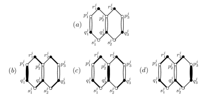
Figure 2: ClauseGadget

We complete the construction by adding edges from vertex gadgets to appropriate clause gadget portals. Specifically, (i) if the $k$-th literal in clause $D^{j}$ is $V^{i}$, then we add edges from $v^{i}_{2j}$ to $p^{j}_{k}$ and $q^{j}_{k}$ to $w^{i}_{2j}$ (cf. Figure 3(a)) and (ii) if the $k$-th literal in clause $D^{j}$ is $\overline{V^{i}}$, then we add edges from $v^{i}_{2j}$ to $p^{j}_{k}$ and $q^{j}_{k}$ to $w^{i}_{2j-1}$ (cf. Figure 3(b)). These connector edges, shown dashed in Figures 3(a) and (b), are forbidden in any matching satisfying the constraints set out above, by the inclusion, for each such edge, of a pair of additional vertices and associated bridging path, as illustrated in Figure 3(c). (Observe that since the graph has the same number of black and white vertices, a matching that saturates all of the black vertices must also saturate all of the white vertices. Thus, for each connector edge, the middle edge of its bridging path is forced to belong to the matching; otherwise, the end edges of the bridging path must both be chosen, resulting in a clash.)

It follows that if the $k$-th literal in clause $D^{j}$ is $V^{i}$, and the edge $p^{j}_{k}q^{j}_{k}$ belongs to the constrained matching then edge $v^{i}_{2j}w^{i}_{2j}$ cannot belong. Similarly, if the $k$-th literal in clause $D^{j}$ is $\overline{V^{i}}$, and the edge $p^{j}_{k}q^{j}_{k}$ belongs to the constrained matching then edge $v^{i}_{2j}w^{i}_{2j-1}$ cannot belong.

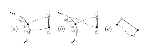
Figure 3: Connector Gadgets

To complete the proof it remains to argue that the resulting graph $B_{\cal D}$ admits a matching $M$ such that (i) $M$ saturates all of the black vertices, and (ii) no two edges of $M$ are part of a $4$-cycle in $B_{\cal D}$, if and only if the instance $\cal D$ is satisfiable. Suppose first that $B_{\cal D}$ admits such a matching $M$. Since none of the connector edges are included in $M$, it follows (as argued above) that in every vertex gadget the black vertices are saturated in one of the two ways illustrated in Figure 1(b) and 1(c)). Similarly, in every clause gadget, the black vertices are saturated in one of the three ways illustrated in Figure 2(b), 2(c) and 2(d)). Suppose that the portal edge $p^{j}_{k}q^{j}_{k}$ of the gadget associated with clause $D^{j}$ belongs to the matching $M$. Then, by our choice of connector edges, if the $k$-th literal in clause $D_{j}$ is $V^{i}$, it must be that edge $v^{i}_{2j}w^{i}_{2j}$ does not belong to $M$, that is the matching on the variable gadget associated with $V^{i}$ has the associated truth assignment $\tt true$. Similarly, if the $k$-th literal in clause $D_{j}$ is $\overline{V^{i}}$, it must be that edge $v^{i}_{2j}w^{i}_{2j-1}$ does not belong to $M$, that is the matching on the variable gadget associated with $V^{i}$ has the associated truth assignment $\tt false$. It follows that the truth assignment to the variables in $\cal V$, associated with the matchings induced on the vertex gadgets, satisfies all of the clauses in $\cal D$.

On the other hand, suppose that $\cal D$ is satisfiable, that is there is an assignment of truth values to the variables in $\cal V$ that satisfies all of the clauses in $\cal D$. Then, if we (i) choose the matching on the vertex gadget associated with $V^{i}$ to be the one corresponding to its truth assignment, and (ii) choose any matching on the clause gadget associated with clause $D^{j}$ including a portal edge associated with one of the satisfied literals in $D^{j}$, and (iii) choose all of the edges added to prevent the choice of connector edges, it is straightforward to confirm that the chosen edges form a matching $M$ in $B_{\cal D}$ such that (i) $M$ saturates all of the black vertices, and (ii) no two edges of $M$ are part of a $4$-cycle in $B_{\cal D}$.  

B Complexity of Degree-bounded Instances of Non-clashing Bipartite Matching

The reduction described in the proof of Theorem 34 produces a bipartite graph whose vertices have degree at most five. (Degree five is attained for the vertices $p^{j}_{2}$ and $q^{j}_{2}$ of the clause gadgets, both of which have three incident edges within the gadget and two from a bridged connector.) It is natural to ask if the hardness result continues to hold for bipartite graphs all of whose vertices have degree strictly less than five. In the next subsection we describe a fairly simple modification of both our clause and connector structures that allows us to reduce the maximum degree to three. Following that, we show that if the maximum degree among vertices in either part of a given bipartite graph is reduced to two there is a polynomial time algorithm to decide if the graph admits a non-clashing matching.

B.1 A modified reduction with maximum degree three

We begin by describing a new clause gadget, illustrated in Figure 4(a), with the same $p$-$q$ portal structure as before but with the additional property that all $p$ and $q$ vertices have degree two. It is straightforward to confirm that, up to symmetry, the matching illustrated in Figure 4(b) is the only matching that saturates all of the vertices using only edges internal to the gadget.

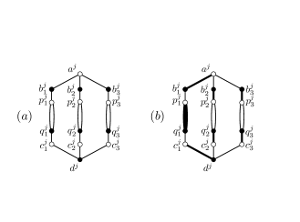
Figure 4: NewClauseGadget

Next we describe a somewhat more complicated connector structure that is used to link vertices in the variable gadgets with portal vertices of the new clause gadget. Schematically, as illustrated in Figures 5(a) and (b), the connector structure plays exactly the same role as its counterpart (pair of bridged edges) in the earlier construction. The new connector structure, illustrated in Figures 5(c), also contains edges, dashed as before, that cannot be part of any perfect non-clashing matching. Their role, as before, is simply to constrain the choice of other edges (in any perfect non-clashing matching).

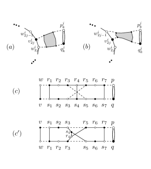
Figure 5: NewConnectorGadgets

It is easiest to argue first that neither of the dashed diagonals can be used. If both are used then edge $r_{4}s_{4}$ must also be used, creating a clash. On the other hand if just one, say $r_{3}s_{5}$ is used, then either $r_{4}s_{4}$ must also be used or both $r_{4}r_{5}$ and $s_{3}s_{4}$ must be used, creating a clash in either case.

By parity, an even number of the horizontal dashed edges are used in any perfect matching. Since it is impossible to choose both $wr_{1}$ and $vs_{1}$ (or both $r_{7}p$ and $s_{7}q$) in a non-clashing matching, it suffices to rule out the case where exactly one of $wr_{1}$ and $vs_{1}$ and exactly one of $r_{7}p$ and $s_{7}q$ belong to a perfect matching. Suppose $r_{7}p$ (but not $s_{7}q$) is chosen. Then the matching is forced to include $r_{5}r_{6}$ and $s_{6}s_{7}$ (in order to saturate $r_{6}$ and $s_{7}$). This in turn forces the choice of $r_{3}r_{4}$ and $s_{4}s_{5}$ (in order to saturate $r_{4}$ and $s_{5}$), creating a clash. By symmetry, it follows that none of the horizontal dashed edges can be used in a perfect non-clashing matching.

It remains to argue that (i) if a non-clashing matching contains edge $pq$ then edge $vw$ cannot belong (and vice versa); (ii) there is a non-clashing matching of the connector gadget that contains edge $pq$ but leaves both $v$ and $w$ exposed (and vice versa); and (iii) there is a non-clashing matching of the connector gadget that leaves all of $v$, $w$, $p$ and $q$ exposed. For (i), we observe that, by chained forcing as above, the inclusion of $pq$ forces the inclusion of $r_{1}s_{1}$ (and, by symmetry, the inclusion of $vw$ forces the inclusion of $r_{7}s_{7}$). Properties (ii) and (iii) are illustrated in Figure 6.

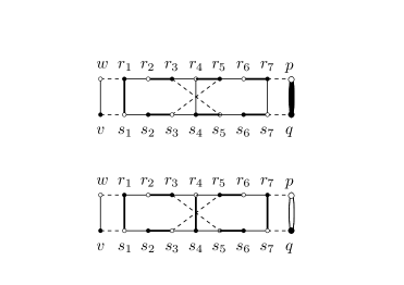
Figure 6: ConnectorMatchings

B.2 An efficient algorithm for Non-Clashing Bipartite Matching, when the maximum degree on either part is at most two

Suppose we are given a bipartite graph $B$ whose vertices are either black or white, and all edges join a black vertex to a white vertex. We want to determine if $B$ admits a matching $M$ such that (i) $M$ saturates all of the black vertices, and (ii) no two edges of $M$ are part of a $4$-cycle in $B$.

Suppose further that the vertices on one of the two parts of $B$ all have degree at most two. We can assume, without loss of generality that they all have degree exactly two, since edges with an endpoint of degree one can be (incrementally) included in a maximum matching $M$ without risk of being part of a $4$-cycle in $B$.

We say that a pair of vertices in this degree-bounded part are twins if they have the same adjacent vertices. We can assume that $B$ has no twins since (i) twins cannot both be saturated without producing a forbidden $4$-cycle, and therefore (ii) the existence of black twins immediately precludes a non-clashing matching, and (iii) any pair of white twins can be replaced by a single copy of the twinned vertex.

With this simplification it is easy to confirm that any matching that saturates the black vertices, the existence of which can be determined in polynomial time, must be non-clashing,

References

- Angluin (1980) Dana Angluin. Inductive inference of formal languages from positive data. Information and Control, 45(2):117–135, 1980.
- Argall et al. (2009) Brenna Argall, Sonia Chernova, Manuela M. Veloso, and Brett Browning. A survey of robot learning from demonstration. Robotics and Autonomous Systems, 57(5):469–483, 2009.
- Balbach (2008) Frank Balbach. Measuring teachability using variants of the teaching dimension. Theoretical Computer Science, 397(1–3):94–113, 2008.
- Bengio et al. (2009) Yoshua Bengio, Jérôme Louradour, Ronan Collobert, and Jason Weston. Curriculum learning. In Proceedings of the 26th Annual International Conference on Machine Learning, ICML, pages 41–48, 2009.
- Cechlárová (1991) Katarina Cechlárová. The uniquely solvable bipartite matching problem. Operations Research Letters, 10(4):221–224, 1991.
- Chalopin et al. (2018) Jérémie Chalopin, Victor Chepoi, Shay Moran, and Manfred K. Warmuth. Unlabeled sample compression schemes and corner peelings for ample and maximum classes. ArXiv, abs/1812.02099, 2018. URL http://arxiv.org/abs/1812.02099.
- Darnstädt et al. (2016) Malte Darnstädt, Thorsten Kiss, Hans Ulrich Simon, and Sandra Zilles. Order compression schemes. Theor. Comput. Sci., 620:73–90, 2016.
- Denis (2001) François Denis. Learning regular languages from simple positive examples. Machine Learning, 44(1/2):37–66, 2001.
- Doliwa et al. (2014) Thorsten Doliwa, Gaojian Fan, Hans Ulrich Simon, and Sandra Zilles. Recursive teaching dimension, VC-dimension and sample compression. J. Mach. Learn. Res., 15:3107–3131, 2014.
- Floyd and Warmuth (1995) Sally Floyd and Manfred Warmuth. Sample compression, learnability, and the Vapnik-Chervonenkis dimension. Machine Learning, 21(3):1–36, 1995.
- Gao et al. (2017) Ziyuan Gao, Christoph Ries, Hans Ulrich Simon, and Sandra Zilles. Preference-based teaching. J. Mach. Learn. Res., 18(31):1–32, 2017.
- Goldman and Kearns (1995) Sally A. Goldman and Michael J. Kearns. On the complexity of teaching. Journal of Computer and System Sciences, 50(1):20–31, 1995.
- Goldman and Mathias (1996) Sally A. Goldman and H. David Mathias. Teaching a smarter learner. J. Comput. Syst. Sci., 52(2):255–267, 1996.
- Golumbic et al. (2001) Martin C. Golumbic, Tirza Hirst, and Moshe Lewenstein. Uniquely restricted matchings. Algorithmica, 31(2):139–154, 2001.
- Ho et al. (2016) Mark K Ho, Michael Littman, James MacGlashan, Fiery Cushman, and Joseph L Austerweil. Showing versus doing: Teaching by demonstration. In Advances in Neural Information Processing Systems 29 (NIPS), pages 3027–3035. 2016.
- Hu et al. (2017) Lunjia Hu, Ruihan Wu, Tianhong Li, and Liwei Wang. Quadratic upper bound for recursive teaching dimension of finite VC classes. In Proceedings of the 30th Conference on Learning Theory, COLT 2017, Amsterdam, The Netherlands, 7-10 July 2017, pages 1147–1156, 2017.
- Kirkpatrick et al. (2019) David Kirkpatrick, Hans U. Simon, and Sandra Zilles. Optimal collusion-free teaching. In Proceedings of Machine Learning Research (ALT2019), volume 98, 2019.
- Kuzmin and Warmuth (2007) Dima Kuzmin and Manfred K. Warmuth. Unlabeled compression schemes for maximum classes. J. Mach. Learn. Res., 8:2047–2081, 2007.
- Littlestone and Warmuth (1986) Nick Littlestone and Manfred K. Warmuth. Relating data compression and learnability. Technical Report, UC Santa Cruz, 1986.
- Moran and Yehudayoff (2016) Shay Moran and Amir Yehudayoff. Sample compression schemes for VC classes. J. ACM, 63(3):21:1–21:10, 2016.
- Moran et al. (2015) Shay Moran, Amir Shpilka, Avi Wigderson, and Amir Yehudayoff. Teaching and compressing for low VC-dimension. CoRR, abs/1502.06187, 2015.
- Sauer (1972) Norbert Sauer. On the density of families of sets. Journal of Combinatorial Theory, Series A, 13(1):145–147, 1972.
- Schwab et al. (2000) Ingo Schwab, Wolfgang Pohl, and Ivan Koychev. Learning to recommend from positive evidence. In Proceedings of the 5th International Conference on Intelligent User Interfaces, IUI, pages 241–247, 2000.
- Shafto et al. (2014) Patrick Shafto, Noah D. Goodman, and Thomas L. Griffiths. A rational account of pedagogical reasoning: Teaching by, and learning from, examples. Cognitive psychology, 71:55–89, 2014.
- Shinohara and Miyano (1991) Ayumi Shinohara and Satoru Miyano. Teachability in computational learning. New Gen. Comput., 8:337–348, 1991.
- Vapnik and Chervonenkis (1971) Vladimir N. Vapnik and Alexey Ya. Chervonenkis. On the uniform convergence of relative frequencies of events to their probabilities. Theor. Probability and Appl., 16(2):264–280, 1971.
- Wang et al. (2006) Chunlin Wang, Chris H. Q. Ding, Richard F. Meraz, and Stephen R. Holbrook. Psol: a positive sample only learning algorithm for finding non-coding RNA genes. Bioinformatics, 22(21):2590–2596, 2006.
- Wexler and Culicover (1980) Kenneth Wexler and Peter W. Culicover. Formal principles of language acquisition. MIT Press, 1980.
- Zhu et al. (2018) Xiaojin Zhu, Adish Singla, Sandra Zilles, and Anna N. Rafferty. An overview of machine teaching. CoRR, abs/1801.05927, 2018.
- Zilles et al. (2011) Sandra Zilles, Steffen Lange, Robert Holte, and Martin Zinkevich. Models of cooperative teaching and learning. J. Mach. Learn. Res., 12:349–384, 2011.