Rectangular Bounding Process
Rectangular Bounding Process
Abstract
Stochastic partition models divide a multi-dimensional space into a number of rectangular regions, such that the data within each region exhibit certain types of homogeneity. Due to the nature of their partition strategy, existing partition models may create many unnecessary divisions in sparse regions when trying to describe data in dense regions. To avoid this problem we introduce a new parsimonious partition model – the Rectangular Bounding Process (RBP) – to efficiently partition multi-dimensional spaces, by employing a bounding strategy to enclose data points within rectangular bounding boxes. Unlike existing approaches, the RBP possesses several attractive theoretical properties that make it a powerful nonparametric partition prior on a hypercube. In particular, the RBP is self-consistent and as such can be directly extended from a finite hypercube to infinite (unbounded) space. We apply the RBP to regression trees and relational models as a flexible partition prior. The experimental results validate the merit of the RBP in rich yet parsimonious expressiveness compared to the state-of-the-art methods.
1 Introduction
Stochastic partition processes111The code of the paper is provided in https://github.com/xuhuifan/RBP on a product space have found many real-world applications, such as regression trees [5, 18, 22], relational modeling [17, 2, 21], and community detection [26, 16]. By tailoring a multi-dimensional space (or multi-dimensional array) into a number of rectangular regions, the partition model can fit data using these “blocks” such that the data within each block exhibit certain types of homogeneity. As one can choose an arbitrarily fine resolution of partition, the data can be fitted reasonably well.
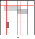
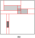
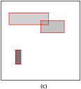
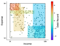
The cost of finer data fitness is that the partition model may induce unnecessary dissections in sparse regions. Compared to the regular-grid partition process [17], the Mondrian process (MP) [32] is more parsimonious for data fitting due to a hierarchical partition strategy; however, the strategy of recursively cutting the space still cannot largely avoid unnecessary dissections in sparse regions. Consider e.g. a regression tree on a multi-dimensional feature space: as data usually lie in some local regions of the entire space, a “regular-grid” or “hierarchical” (i.e. d-tree) partition model would inevitably produce too many cuts in regions where data points rarely locate when it tries to fit data in dense regions (see illustration in the left panel of Figure 1). It is accordingly challenging for a partition process to balance fitness and parsimony.
Instead of this cutting-based strategy, we propose a bounding-based partition process – the Rectangular Bounding Process (RBP) – to alleviate the above limitation. The RBP generates rectangular bounding boxes to enclose data points in a multi-dimensional space. In this way, significant regions of the space can be comprehensively modelled. Each bounding box can be efficiently constructed by an outer product of a number of step functions, each of which is defined on a dimension of the feature space, with a segment of value “1” in a particular interval and “0” otherwise. As bounding boxes are independently generated, the layout of a full partition can be quite flexible, allowing for a simple description of those regions with complicated patterns. As a result, the RBP is able to use fewer blocks (thereby providing a more parsimonious expression of the model) than those cutting-based partition models while achieving a similar modelling capability.
The RBP has several favourable properties that make it a powerful nonparametric partition prior: (1) Given a budget parameter and the domain size, the expected total volume of the generated bounding boxes is a constant. This is helpful to set the process hyperparameters to prefer few large bounding boxes or many small bounding boxes. (2) Each individual data point in the domain has equal probability to be covered by a bounding box. This gives an equal tendency towards all possible configurations of the data. (3) The process is self-consistent in the sense that, when restricting a domain to its sub-domain, the probability of the resulting partition on the sub-domain is the same as the probability of generating the same partition on the sub-domain directly. This important property enables the RBP to be extendable from a hypercube to the infinite multi-dimensional space according to the Kolmogorov extension theorem [6]. This is extremely useful for the domain changing problem setting, such as regression problems over streaming data.
The RBP can be a beneficial tool in many applications. In this paper we specifically investigate (1) regression trees, where bounding boxes can be viewed as local regions of certain labels, and (2) relational modelling, where bounding boxes can be viewed as communities in a complex network. We develop practical and efficient MCMC methods to infer the model structures. The experimental results on a number of synthetic and real-world data sets demonstrate that the RBP can achieve parsimonious partitions with competitive performance compared to the state-of-the-art methods.

2 Related Work
2.1 Stochastic Partition Processes
Stochastic partition processes divide a multi-dimensional space (for continuous data) or a multi-dimensional array (for discrete data) into blocks such that the data within each region exhibit certain types of homogeneity. In terms of partitioning strategy, state-of-the-art stochastic partition processes can be roughly categorized into regular-grid partitions and flexible axis-aligned partitions (Figure 1).
A regular-grid stochastic partition process is constituted by separate partition processes on each dimension of the -dimensional array. The resulting orthogonal interactions between two dimensions produce regular grids. Typical regular-grid partition models include the infinite relational model (IRM) [17] and mixed-membership stochastic blockmodels [2]. Bayesian plaid models [24, 15, 4] generate “plaid” like partitions, however they neglect the dependence between latent feature values and more importantly, they are restricted to discrete arrays (in contrast to our continuous space model). Regular-grid partition models are widely used in real-world applications for modeling graph data [14, 33].
To our knowledge, only the Mondrian process (MP) [32, 31] and the rectangular tiling process (RTP) [25] can produce flexible axis-aligned partitions on a product space. The MP recursively generates axis-aligned cuts on a unit hypercube and partitions the space in a hierarchical fashion known as a d-tree. Compared to the hierarchical partitioning strategy, the RTP generates a flat partition structure on a two-dimensional array by assigning each entry to an existing block or a new block in sequence, without violating the rectangular restriction on the blocks.
2.2 Bayesian Relational Models
Most stochastic partition processes are developed to target relational modelling [17, 32, 25, 36, 9, 10]. A stochastic partition process generates a partition on a multi-dimensional array, which serves as a prior for the underlying communities in the relational data (e.g. social networks in the 2-dimensional case). After generating the partition, a local model is allocated to each block (or polygon) of the partition to characterize the relation type distribution in that block. For example, the local model can be a Bernoulli distribution for link prediction in social networks or a discrete distribution for rating prediction in recommender systems. Finally, row and column indexes are sampled to locate a block in the partition and use the local model to further generate the relational data.
Compared to the existing stochastic partition processes in relational modelling, the RBP introduces a very different partition approach: the RBP adopts a bounding-based strategy while the others are based on cutting-based strategies. This unique feature enables the RBP to directly capture important communities without wasting model parameters on unimportant regions. In addition, the bounding boxes are independently generated by the RBP. This parallel strategy is much more efficient than the hierarchical strategy [32, 9] and the entry-wise growing strategy [25].
2.3 Bayesian Regression Trees
The ensemble of regression/decision trees [3, 11] is a popular tool in regression tasks due to its competitive and robust performance against other models. In the Bayesian framework, Bayesian additive regression trees (BART) [5] and the Mondrian forest [18, 19] are two representative methods.
BART adopts an ensemble of trees to approximate the unknown function from the input space to the output label. Through prior regularization, BART can keep the effects of individual trees small and work as a “weak learner” in the boosting literature. BART has shown promise in nonparametric regression; and several variants of BART have been developed to focus on different scenarios, including heterogeneous BART [29] allowing for various observational variance in the space, parallel BART [30] enabling parallel computing for BART, and Dirichlet additive regression trees [22] imposing a sparse Dirichlet prior on the dimensions to address issues of high-dimensionality.
The Mondrian forest (MF) is built on the idea of an ensemble of Mondrian processes (d-trees) to partition the space. The MF is distinct from BART in that the MF may be more suitable for streaming data scenarios, as the distribution of trees sampled from the MP stays invariant even if the data domain changes over time.
3 The Rectangular Bounding Process
The goal of the Rectangular Bounding Process (RBP) is to partition the space by attaching rectangular bounding boxes to significant regions, where “significance” is application dependent. For a hypercubical domain with denoting the length of the -th dimension of , a budget parameter is used to control the expected number of generated bounding boxes in and a length parameter is used to control the expected size of the generated bounding boxes. The generative process of the RBP is defined as follows:
-
1.
Sample the number of bounding boxes ;
-
2.
For , , sample the initial position and the length of the -th bounding box (denoted as ) in the -th dimension:
-
(a)
Sample the initial position as
(3) -
(b)
Sample the length as
(6)
-
(a)
-
3.
Sample i.i.d. time points uniformly in and index them to satisfy . Set the cost of as ().
Here Trun-Exp refers to an exponential distribution with rate , truncated at . The RBP is defined in a measurable space , where denotes the domain and denotes the collection of all finite boxes in . Each element in denotes a partition of , comprising a collection of rectangular bounding boxes , where indexes the bounding boxes in . A bounding box is defined by an outer product , where is a step function defined on , taking value of “1” in and “0” otherwise (see right panel of Figure 1).
Given a domain , hyperparameters and , a random partition sampled from the RBP can be represented as: . We assume that the costs of bounding boxes are i.i.d. sampled from the same exponential distribution, which implies there exists a homogeneous Poisson process on the time (cost) line. The generating time of each bounding box is uniform in and the number of bounding boxes has a Poisson distribution. We represent a random partition as .
3.1 Expected Total Volume
Proposition 1.
Given a hypercubical domain with denoting the length of the -th dimension of and the value of , the expected total volume of the bounding boxes (i.e. expected number of boxes expected volume of a box) in sampled from a RBP is a constant .
The expected length of the interval in with value “1” is . According to the definition of the RBP (Poisson distribution in Step 1), we have an expected number of bounding boxes in . Thus, the expected total volume of the bounding boxes for a given budget and a domain is .
Proposition 1 implies that, given and , the RBP generates either many small-sized bounding boxes or few large-sized bounding boxes. This provides a practical guidance on how to choose appropriate values of and when implementing the RBP. Given the lengths of , an estimate of the lengths of the bounding boxes can help to choose (i.e. ). An appropriate value of can then be chosen to determine the expected number of bounding boxes.
3.2 Coverage Probability
Proposition 2.
For any data point (including the boundaries of ), the probability of falling in the interval of on is a constant (and does not depend on ). As the step functions for constructing the -th bounding box in are independent, is covered by with a constant probability.
The property of constant coverage probability is particularly suitable for regression problems. Proposition 2 implies there is no biased tendency to favour different data regions in . All data points have equal probability to be covered by a bounding box in a RBP partition .
Another interesting observation can be seen from this property: Although we have specified a direction for generating the -th dimension of in the generative process (i.e. the initial position and the terminal position ), the probability of generating is the same if we reverse the direction of the -th dimension, which is . It is obvious that the joint probability of the initial position and the terminal position is invariant if we reverse the direction of the -th dimension. Direction is therefore only defined for notation convenience – it will not affect the results of any analysis.
3.3 Self-Consistency
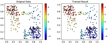
The RBP has the attractive property of self-consistency. That is, while restricting an on -dimensional hypercube , to a sub-domain , , the resulting bounding boxes restricted to are distributed as if they are directly generated on through an (see Figure 2 for an illustration). Typical application scenarios are regression/classification tasks on streaming data, where new data points may be observed outside the current data domain , say falling in , where represents the data domain (minimum bounding box of all observed data) in the future (left panel of Figure 3). Equipped with the self-consistency property, the distribution of the RBP partition on remains invariant as new data points come and expand the data domain.
The self-consistency property can be verified in three steps: (1) the distribution of the number of bounding boxes is self-consistent; (2) the position distribution of a bounding box is self-consistent; (3) the RBP is self-consistent. In the following, we use to denote the projection that restricts to by keeping ’s partition in unchanged and removing the rest.
Proposition 3.
While restricting the to , , we have the following results:
-
1.
The time points of bounding boxes crossing into from follow the same Poisson process for generating the time points of bounding boxes in a . That is .
-
2.
The marginal probability of the pre-images of a bounding box in (given the bounding box in would cross into ) equals the probability of being directly sampled from a . That is, .
- 3.
The generative process provides a way of defining the RBP on a multidimensional finite space (hypercube). According to the Kolmogorov extension theorem ([6]), we can further extend RBP to the multidimensional infinite space .
Theorem 1.
The probability measure on the measurable space of the RBP, , can be uniquely extended to on as the projective limit measurable space.
4 Application to Regression Trees
4.1 RBP-Regression Trees
We apply the RBP as a space partition prior to the regression-tree problem. Given the feature and label pairs , the bounding boxes sampled from an RBP on the domain of the feature data are used for modelling the latent variables that influence the observed labels. Since the allow for a partition layout of overlapped bounding boxes, each single feature point can be covered by more than one bounding box, whose latent variables together form an additive effect to influence the corresponding label.
The generative process for the RBP-regression tree is as follows:

4.2 Sampling for RBP-Regression Tree
The joint probability of the label data , the number of bounding boxes , the variables related to the bounding boxes , and the error variance is
We adopt MCMC methods to iteratively sampling from the resulting posterior distribution.
Sample : We use a similar strategy to [1] for updating . We accept the addition or removal of a bounding box with an acceptance probability of or respectively, where
, , and (or ) denotes the probability of proposing to add (or remove) a bounding box.
Sample :
Both and can be sampled through Gibbs sampling:
where , , and is the number of data points belonging to the -th bounding box.
Sample :
To update we use the Metropolis-Hastings algorithm, generating the proposed (which determine ) using the RBP generative process (Step 2.(a)(b)). Thus, the acceptance probability is based purely on the likelihoods for the proposed and current configurations.
4.3 Experiments
We empirically test the RBP regression tree (RBP-RT) for the regression task. We compare the RBP-RT with several state-of-the-art methods: (1) a Bayesian additive regression tree (BART) [5]; (2) a Mondrian forest (MF) [18, 19]; (3) a random forest (RF) [3]; and (4) an extremely randomized tree (ERT) [12]. For BART, we implement a particle MCMC strategy to infer the structure of each tree in the model; for the MF, we directly use the existing code provided by the author222https://github.com/balajiln/mondrianforest; for the RF and ERT, we use the implementations in the scikit-learn toolbox [28].
Synthetic data:
We first test the RBP-RT on a simple synthetic data set. A total of bounding boxes are assigned to the unit square , each with its own mean intensity . From each bounding box points are uniformly sampled, with the label data generated from a normal distribution, with mean the sum of the intensities of the bounding boxes covering the data point, and standard deviation . In this way, a total of data points are generated in .
To implement the RBP-TR we set the total number of iterations to , (i.e. the expected box length is ) and (i.e. the expected number of bounding boxes is ). It is worth noting that is a relatively small number of blocks when compared to the other state-of-the-art methods. For instance, BART usually sets the number of trees to be at least and there are typically more than blocks in each tree (i.e. at least blocks in total). The right panel of Figure 3 shows a visualization of the data fitting result of the RBP regression-tree.
Real-world data:
We select several real-world data sets to compare the RBP-RT and the other state-of-the-art methods: Protein Structure [8] (), Naval Plants [7] (), Power Plants [34] (), Concrete [37] (), and Airfoil Self-Noise [8] (). Here, we first use PCA to select the largest components and then normalize them so that they lie in the unit hypercube for ease of implementation. As before, we set the total number of iterations to 500, and this time set (i.e. the expected number of bounding boxes is ).
The resulting Residual Mean Absolute Errors (RMAE) are reported in Table 1. In general, the three Bayesian tree ensembles perform worse than the random forests. This may in part be due to the maturity of development of the RF algorithm toolbox. While the RBP-RT does not perform as well as the random forests, its performance is comparable to that of BART and MF (sometimes even better), but with many fewer bounding boxes (i.e. parameters) used in the model, clearly demonstrating its parsimonious construction.
| Data Sets | RF | ERT | BART | MF | RBP-RT |
|---|---|---|---|---|---|
| Protein | |||||
| Naval Plants | |||||
| Power Plants | |||||
| Concrete Data | |||||
| Airfoil self-noise |
5 Application to Relational Modeling
5.1 The RBP-Relational Model
Another possible application of the RBP is in relational modeling. Given relational data as an asymmetric matrix , with indicating the relation from node to node , the bounding boxes with rates belonging to a partition may be used to model communities with different intensities of relations.
The generative process of an RBP relational model is as follows: (1) Generate a partition on ; (2) for , generate rates ; (3) for , generate the row and column coordinates ; (4) for , generate relational data , where is the logistic function, mapping the aggregated relation intensity from to . While here we implement a RBP relational model with binary interactions (i.e. the Bernoulli likelihood), other types of relations (e.g. categorical likelihoods) can easily be accommodated.
Together, the RBP and the mapping function play the role of the random function defined in the graphon literature [27]. Along with the uniformly generated coordinates for each node, the RBP relational model is expected to uncover homogeneous interactions in as compact boxes.
5.2 Sampling for RBP-Relational Model
The joint probability of the label data , the number of bounding boxes , the variables related to the bounding boxes , and the coordinates for the nodes (with in the RBP relational model) is
We adopt MCMC methods to iteratively sample from the resulting posterior distribution.
Sample : We use a similar strategy to [1] for updating . We accept the addition or removal of a bounding box with an acceptance probability of or respectively, where
where , and (or ) denotes the probability of proposing to add (or remove) a bounding box.
Sample :
For the -th box, , a new is sampled from the proposal distribution . We then accept with probability , where
Sample :
This update is the same as for the RBP-regression tree sampler (Section 4.2).
Sample
We propose new values from the uniform prior distribution. Thus, the acceptance probability is purely based on the likelihoods of the proposed and current configurations.
5.3 Experiments
| Data Sets | IRM | LFRM | MP-RM | BSP-RM | MTA-RM | RBP-RM |
|---|---|---|---|---|---|---|
| Digg | ||||||
| Flickr | ||||||
| Gplus | ||||||
We empirically test the RBP relational model (RBP-RM) for link prediction. We compare the RBP-RM with four state-of-the-art relational models: (1) IRM [17] (regular grids); (2) LFRM [24] (plaid grids); (3) MP relational model (MP-RM) [32] (hierarchical d-tree); (4) BSP-tree relational model (BSP-RM) [9]; (5) Matrix tile analysis relational model (MTA-RM) [13] (noncontiguous tiles). For inference on the IRM and LFRM, we adopt collapsed Gibbs sampling algorithms, for MP-RM we use reversible-jump MCMC [35], for BSP-RM we use particle MCMC, and for MTA-RM we implement the iterative conditional modes algorithm used in [13].
Data Sets: Five social network data sets are used: Digg, Flickr [38], Gplus [23], Facebook and Twitter [20]. We extract a subset of nodes (the top 1000 active nodes based on their interactions with others) from each data set for constructing the relational data matrix.
Experimental Setting: The hyper-parameters for each method are set as follows: In IRM, we let the concentration parameter be sampled from a gamma prior, and the row and column partitions be sampled from two independent Dirichlet processes; In LFRM, we let be sampled from a gamma prior. As the budget parameter for MP-RM and BSP-RM is hard to sample [19], we set it to , implying that around blocks would be generated. For the parametric model MTA-RM, we simply set the number of tiles to 16; In RBP-RM, we set and , which leads to an expectation of boxes. The reported performance is averaged over 10 randomly selected hold-out test sets (Train:Test = 9:1).
Results: Table 2 reports the link prediction performance comparisons for each method and datasets. We see that the RBP-RM achieves competitive performance against the other methods. Even on the data sets it does not obtain the best score, its performance is comparable to the best. The overall results validate that the RBP-RM is effective in relational modelling due to its flexible and parsimonious construction, attaching bounding boxes to dense data regions.
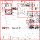
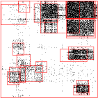
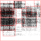
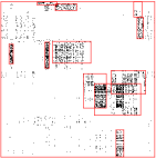
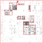
Figure 4 visually illustrates the RBP-RM partitions patterns for each dataset. As is apparent, the bounding-based RBP-RM method indeed describing dense regions of relational data matrices with relatively few bounding boxes (i.e. parameters). An interesting observation from this partition format, is that the overlapping bounding boxes are very useful for describing inter-community interactions (e.g. overlapping bounding boxes in Digg, Flickr, and Gplus) and community-in-community interactions (e.g. upper-right corner in Flickr and Gplus). Thus, in addition to competitive and parsimonious performance, the RBP-RM also produces intuitively interpretable and meaningful partitions (Figure 4).
6 Conclusion
We have introduced a novel and parsimonious stochastic partition process – the Rectangular Bounding Process (RBP). Instead of the typical cutting-based strategy of existing partition models, we adopt a bounding-based strategy to attach rectangular bounding boxes to model dense data regions in a multi-dimensional space, which is able to avoid unnecessary dissections in sparse data regions. The RBP was demonstrated in two applications: regression trees and relational modelling. The experimental results on these two applications validate the merit of the RBP, that is, competitive performance against existing state-of-the-art methods, while using fewer bounding boxes (i.e. fewer parameters).
Acknowledgements
Xuhui Fan and Scott A. Sisson are supported by the Australian Research Council through the Australian Centre of Excellence in Mathematical and Statistical Frontiers (ACEMS, CE140100049), and Scott A. Sisson through the Discovery Project Scheme (DP160102544). Bin Li is supported by Fudan University Startup Research Grant and Shanghai Municipal Science & Technology Commission (16JC1420401).
Appendix A Calculation of the expected side length in Proposition 1
The expected length of the interval in with value “1” is (some super/subscripts are omitted in this proof for conciseness):
where the first term after refers to the expected length of the interval when starting at and the second term refers to the expected length when starting from a point larger than . We need to use the equality in the above derivation.
Appendix B Proof for Proposition 2 (Coverage Probability)
For any data point (including the boundaries of ), the probability of falling in the interval of on is a constant (some super/subscripts are omitted in this proof for conciseness).
If locates on the initial boundary, i.f.f. , which is
| (8) |
If , we have the corresponding probability as
Appendix C Proof for Proposition 3 (Self-Consistency)
Proposition 3.1: The number distribution of bounding boxes is self-consistent
Proof.
According to the definition of Poisson process, the bounding boxes sampled from (or ) follow a homogeneous Poisson process with intensity (or ). Given the same budget , the result holds if we can prove the following equality of the two Poisson process intensities
| (10) |
Due to the independence of dimensions, can be rewritten as
| (11) |
where we use to denote the case that the step function would take value “1” in an interval of the -th dimension of domain .
W.l.o.g, we assume that the two domains, and , have the same shape apart from the -th dimension where the length of dimension in is larger than that of in .
There are three cases to consider: (1) and share the terminal boundary in the -th dimension; (2) and share the initial boundary in the -th dimension; (3) and do not share the boundaries in the -th dimension. Proving case (1) and case (2) together would obviously lead to case (3). In either case, by independence of dimensions, we need to prove the following equation.
| (12) |
In case (1) where and share the terminal boundary in the th dimension, we have
where the first term after corresponds to the probability that locates directly in the interval of , the second term corresponds to the probability that locates on the initial boundary and has the length larger than , and the third term corresponds to the probability that locates in the interval of (excluding the initial boundary) and has the length larger than .
In case (2) where and share the initial boundary in the th dimension, we have
| (14) |
since requires the condition of because would lead to the result that .
The conclusion can be derived as above. ∎
Because of the same Poisson process intensity Eq. (10), the following equality also holds
| (15) |
Proposition 3.2: The position distribution of a bounding box is self-consistent
Proof.
W.l.o.g, we assume that the two domains, and , have the same shape apart from the th dimension where has additional space of length () (the general case follows by induction). For dimensions , it is obvious that the law of bounding boxes are consistent under projection because the projection is the identity. Given the same budget , The result holds if we can prove the following equality
| (16) |
There are two cases to consider: (1) and share the initial boundary in the th dimension; (2) and share the terminal boundary in the th dimension. In each case, there are two cases (denoted as A & B in the following) regarding whether the terminal/initial (for Case 1/2, respectively) position locates on the boundary of . In total we have four cases to discuss as follows.
In case (1) where and share the initial boundary, according to Eq. (14), we have .
For convenience of notation, we let , specifically if ; if .
[Case 1.A] For ,
| (17) |
[Case 1.B] For ,
| (18) |
In case (2) where and share the terminal boundary, according to Eq. (C), we have .
[Case 2.A] For , we have . What is more, we have
| (19) | ||||
Thus we can get
| (20) | ||||
where if ; if .
[Case 2.B] For , we have ,
| (21) | ||||
Consider all dimensions, for each case, we have . ∎
Proposition 3.3: RBP is self-consistent
References
- [1] Ryan P. Adams, Iain Murray, and David J.C. MacKay. Tractable nonparametric Bayesian inference in Poisson processes with Gaussian process intensities. In ICML, pages 9–16, 2009.
- [2] Edoardo M. Airoldi, David M. Blei, Stephen E. Fienberg, and Eric P. Xing. Mixed membership stochastic blockmodels. In NIPS, pages 33–40, 2009.
- [3] Leo Breiman. Random forests. Machine Learning, 45(1):5–32, 2001.
- [4] José Caldas and Samuel Kaski. Bayesian biclustering with the plaid model. In MLSP 2008. IEEE Workshop on, pages 291–296. IEEE, 2008.
- [5] Hugh A. Chipman, Edward I. George, and Robert E. McCulloch. Bart: Bayesian additive regression trees. The Annals of Applied Statistics, 4(1):266–298, 2010.
- [6] Kai-Lai Chung. A Course in Probability Theory. Academic Press, 2001.
- [7] Andrea Coraddu, Luca Oneto, Aessandro Ghio, Stefano Savio, Davide Anguita, and Massimo Figari. Machine learning approaches for improving condition-based maintenance of naval propulsion plants. Proceedings of the Institution of Mechanical Engineers, Part M: Journal of Engineering for the Maritime Environment, 230(1):136–153, 2016.
- [8] Dua Dheeru and Efi Karra Taniskidou. UCI machine learning repository, 2017.
- [9] Xuhui Fan, Bin Li, and Scott A. Sisson. The binary space partitioning-tree process. In AISTATS, volume 84, pages 1859–1867. PMLR, 2018.
- [10] Xuhui Fan, Bin Li, Yi Wang, Yang Wang, and Fang Chen. The Ostomachion Process. In AAAI, pages 1547–1553, 2016.
- [11] Yoav Freund, Robert Schapire, and Naoki Abe. A short introduction to boosting. Journal-Japanese Society For Artificial Intelligence, 14(771-780):1612, 1999.
- [12] Pierre Geurts, Damien Ernst, and Louis Wehenkel. Extremely randomized trees. Machine learning, 63(1):3–42, 2006.
- [13] Inmar Givoni, Vincent Cheung, and Brendan Frey. Matrix tile analysis. In UAI, pages 200–207, 2006.
- [14] Katsuhiko Ishiguro, Tomoharu Iwata, Naonori Ueda, and Joshua B. Tenenbaum. Dynamic infinite relational model for time-varying relational data analysis. In NIPS, pages 919–927, 2010.
- [15] Katsuhiko Ishiguro, Issei Sato, Masahiro Nakano, Akisato Kimura, and Naonori Ueda. Infinite plaid models for infinite bi-clustering. In AAAI, pages 1701–1708, 2016.
- [16] Brian Karrer and Mark E.J. Newman. Stochastic blockmodels and community structure in networks. Physical Review E, 83(1):016107, 2011.
- [17] Charles Kemp, Joshua B. Tenenbaum, Thomas L. Griffiths, Takeshi Yamada, and Naonori Ueda. Learning systems of concepts with an infinite relational model. In AAAI, volume 3, pages 381–388, 2006.
- [18] Balaji Lakshminarayanan, Daniel M. Roy, and Yee Whye Teh. Mondrian forests: Efficient online random forests. In NIPS, pages 3140–3148, 2014.
- [19] Balaji Lakshminarayanan, Daniel M. Roy, and Yee Whye Teh. Mondrian forests for large-scale regression when uncertainty matters. In AISTATS, pages 1478–1487, 2016.
- [20] Jure Leskovec, Daniel Huttenlocher, and Jon Kleinberg. Predicting positive and negative links in online social networks. In WWW, pages 641–650, 2010.
- [21] Bin Li, Qiang Yang, and Xiangyang Xue. Transfer learning for collaborative filtering via a rating-matrix generative model. In ICML, pages 617–624, 2009.
- [22] Antonio R Linero. Bayesian regression trees for high-dimensional prediction and variable selection. Journal of the American Statistical Association, pages 1–11, 2018.
- [23] Julian J. McAuley and Jure Leskovec. Learning to discover social circles in ego networks. In NIPS, pages 548–556, 2012.
- [24] Kurt Miller, Michael I. Jordan, and Thomas L. Griffiths. Nonparametric latent feature models for link prediction. In NIPS, pages 1276–1284, 2009.
- [25] Masahiro Nakano, Katsuhiko Ishiguro, Akisato Kimura, Takeshi Yamada, and Naonori Ueda. Rectangular tiling process. In ICML, pages 361–369, 2014.
- [26] Krzysztof Nowicki and Tom A.B. Snijders. Estimation and prediction for stochastic block structures. Journal of the American Statistical Association, 96(455):1077–1087, 2001.
- [27] Peter Orbanz and Daniel M Roy. Bayesian models of graphs, arrays and other exchangeable random structures. IEEE Transactions on Pattern Analysis and Machine Intelligence, 37(2):437–461, 2015.
- [28] F. Pedregosa, G. Varoquaux, A. Gramfort, V. Michel, B. Thirion, O. Grisel, M. Blondel, P. Prettenhofer, R. Weiss, V. Dubourg, J. Vanderplas, A. Passos, D. Cournapeau, M. Brucher, M. Perrot, and E. Duchesnay. Scikit-learn: Machine learning in Python. Journal of Machine Learning Research, 12:2825–2830, 2011.
- [29] Matthew Pratola, Hugh Chipman, Edward George, and Robert McCulloch. Heteroscedastic bart using multiplicative regression trees. arXiv preprint arXiv:1709.07542, 2017.
- [30] Matthew T Pratola, Hugh A Chipman, James R Gattiker, David M Higdon, Robert McCulloch, and William N Rust. Parallel bayesian additive regression trees. Journal of Computational and Graphical Statistics, 23(3):830–852, 2014.
- [31] Daniel M. Roy. Computability, Inference and Modeling in Probabilistic Programming. PhD thesis, MIT, 2011.
- [32] Daniel M. Roy and Yee Whye Teh. The Mondrian process. In NIPS, pages 1377–1384, 2009.
- [33] Mikkel N. Schmidt and Morten Mørup. Nonparametric Bayesian modeling of complex networks: An introduction. IEEE Signal Processing Magazine, 30(3):110–128, 2013.
- [34] Pınar Tüfekci. Prediction of full load electrical power output of a base load operated combined cycle power plant using machine learning methods. International Journal of Electrical Power & Energy Systems, 60:126 – 140, 2014.
- [35] Pu Wang, Kathryn B. Laskey, Carlotta Domeniconi, and Michael I. Jordan. Nonparametric Bayesian co-clustering ensembles. In SDM, pages 331–342, 2011.
- [36] Yi Wang, Bin Li, Yang Wang, and Fang Chen. Metadata dependent Mondrian processes. In ICML, pages 1339–1347, 2015.
- [37] I. Cheng Yeh. Modeling of strength of high-performance concrete using artificial neural networks. Cement and Concrete research, 28(12):1797–1808, 1998.
- [38] Reza Zafarani and Huan Liu. Social computing data repository at ASU, 2009.