Quantifying non-Markovianity: a quantum resource-theoretic approach

Abstract

The quantification and characterization of non-Markovian dynamics in quantum systems is essential both for the theory of open quantum systems and for a deeper understanding of the effects of non-Markovian noise on quantum technologies. Here, we introduce the robustness of non-Markovianity, an operationally-motivated, optimization-free measure that quantifies the minimum amount of Markovian noise that can be mixed with a non-Markovian evolution before it becomes Markovian. We show that this quantity is a bonafide non-Markovianity measure, since it is faithful, convex, and monotonic under composition with Markovian maps. A two-fold operational interpretation of this measure is provided, with the robustness measure quantifying an advantage in both a state discrimination and a channel discrimination task. Moreover, we connect the robustness measure to single-shot information theory by using it to upper bound the min-accessible information of a non-Markovian map. Furthermore, we provide a closed-form analytical expression for this measure and show that, quite remarkably, the robustness measure is exactly equal to half the Rivas-Huelga-Plenio (RHP) measure [Phys. Rev. Lett. 105, 050403 (2010)]. As a result, we provide a direct operational meaning to the RHP measure while endowing the robustness measure with the physical characterizations of the RHP measure.

Introduction.—The idealization of a quantum system coupled to a memoryless environment is exactly that: an idealization. In the theory of open quantum systems, memoryless or Markovian evolution arises from the assumptions of weak (or singular) coupling to a fast bath Breuer and Petruccione (2002); Rivas and Huelga (2012). Although extremely useful, this assumption does not always apply to physical systems of interest—including, but not limited to, several quantum information processing technologies—and so a complete physical picture cannot neglect non-Markovian effects. Quantum non-Markovianity has several distinct definitions and characterizations (see Refs. Rivas et al. (2014); Breuer et al. (2016) for a detailed comparison), prominent examples include the semigroup formulation Alicki and Lendi (2007), the distinguishability measure Breuer et al. (2009), and CP-divisibility Rivas et al. (2010). In this paper, we use the CP-divisibility approach to non-Markovianity.

More formally, the time evolution of a quantum dynamical system is called Markovian (or divisible Wolf and Cirac (2008)) if there exists a family of trace-preserving linear maps, $\{\Lambda_{(t_{2},t_{1})},t_{2}\geq t_{1}\geq t_{0}\}$ which satisfy the composition law, $\Lambda_{\left(t_{3},t_{1}\right)}=\Lambda_{\left(t_{3},t_{2}\right)}\circ\Lambda_{\left(t_{2},t_{1}\right)},\quad t_{3}\geqslant t_{2}\geqslant t_{1}$, where $\Lambda_{(t_{2},t_{1})}$ is a CP map for every $t_{2}$ and $t_{1}$. Quantum systems undergoing Markovian dynamics are described by a master equation, as captured by the following fundamental result.

Definition 1 (Gorini-Kossakowski-Sudarshan-Lindblad Kossakowski (1972); Lindblad (1976); Gorini et al. (1976)).

An operator $\mathcal{L}_{t}$ is the generator of a quantum Markov (or divisible) process if and only if it can be written in the form

$$\frac{\mathrm{d}\rho(t)}{\mathrm{d}t}=\mathcal{L}_{t}[\rho(t)]=-\mathrm{i}[H(t),\rho(t)]\leavevmode\nobreak\ +$$

$$\sum_{k}\gamma_{k}(t)\left[V_{k}(t)\rho(t)V_{k}^{\dagger}(t)-\frac{1}{2}\left\{V_{k}^{\dagger}(t)V_{k}(t),\rho(t)\right\}\right],$$ (1)

where $H(t)$ and $V_{k}(t)$ are time-dependent operators, with $H(t)$ self-adjoint, and $\gamma_{k}(t)\geq 0$ for every $k$ and $t$.

Recently, there has been some effort to characterize, both qualitatively and quantitatively, the resourcefulness of non-Markovianity in quantum information processing tasks Laine et al. (2015), quantum thermodynamics Thomas et al. (2018), quantum error-suppression techniques like dynamical decoupling Addis et al. (2015), and the degree of entanglement that can be generated between a system and the environment Mirkin et al. (2019). However, quantum information theory already has a powerful formalism to characterize the quantification and manipulation of a quantum resource, the so-called quantum resource theories framework Chitambar and Gour (2019). In this paper, we analyze quantum non-Markovianity through the lens of quantum resource theories.

The construction of operational measures for quantum resources is one of the many goals of quantum resource theories. In this direction, there has been a lot of exciting work recently, especially with regard to the so-called robustness measures, which characterize how robust a resource is with respect to “mixing.” Robustness measures with operational significance have been constructed for quantum entanglement Plenio and Virmani (2005), coherence Aberg (2006); Baumgratz et al. (2014); Streltsov et al. (2017), asymmetry Napoli et al. (2016), and other resources. Notably, it was recently shown that for any quantum resource that forms a convex resource theory, there exists a subchannel discrimination game where that resource provides an advantage that is quantified by a generalized robustness measure Takagi et al. (2019). These results were further generalized to arbitrary convex resource theories—both in quantum mechanics and general probabilistic theories—characterizing the resource content not only of quantum states but also of quantum measurements and channels Takagi and Regula (2019) (see also related work by Refs. Skrzypczyk and Linden (2019); Uola et al. (2019)).

Motivated by the operational nature of robustness measures in quantum resource theories, we construct a robustness measure for non-Markovianity, which quantifies the minimum amount of Markovian “noise” that needs to be mixed (in the sense of convex combination) with a non-Markovian process to make it Markovian. A few remarks are in order before we go into more detail, especially about the nature of this resource. Quantum non-Markovianity is a dynamic resource, as opposed to static resources like coherence, entanglement, magic, etc. Static resources are a property of quantum states while dynamic resources are a property of a quantum process. There are two general ways to quantify the resourcefulness of quantum operations. One can either quantify the so-called resource generating power of these operations by relating them to an underlying resource theory of quantum states. Or, one can define an arbitrary set of quantum operations as free and quantify the resourcefulness with respect to this set. In our resource-theoretic construction for non-Markovianity, we take the latter approach, and, as a result, there are no free states, per se; in contrast to the typical approach in static quantum resource theories .

A third construction to quantify the resourcefulness of quantum operations would be to define the set of free superoperations (or free supermaps Chiribella et al. (2008)), which are transformations that leave the set of free operations invariant, and may induce a preorder Chitambar and Gour (2019) over this set. Such a construction would be a proper resource theory since there are both free objects (quantum maps) and free transformations (quantum supermaps). We briefly discuss this possibility for the resource theory of non-Markovianity and show that our choice of free superoperations induces a preorder over the set of all quantum operations (Markovian and non-Markovian).

Preliminaries.—Let $\mathcal{H}$ be a finite-dimensional Hilbert space. Then, consider the (normalized) maximally entangled state between two copies of the Hilbert space, $|\Phi^{+}\rangle=\frac{1}{\sqrt{d}}\sum_{i=0}^{d-1}|i\rangle|i\rangle$, where $d$ is the dimension and $\{|i\rangle\}_{i=0}^{d-1}$ an orthonormal basis for the Hilbert space. To a linear map $\Lambda\mathrel{\mathop{\mathchar 58\relax}}\mathcal{H}\rightarrow\mathcal{H}$, we associate a Choi-Jamiołkowski matrix (called a Choi matrix for brevity), $\rho_{\Lambda}\equiv\left[\mathbb{I}\otimes\Lambda\right]\left(|\Phi^{+}\rangle\langle\Phi^{+}|\right)$. Then, $\rho_{\Lambda}$ is positive-semidefinite if and only if the map $\Lambda$ is completely positive Choi (1975); Jamiołkowski (1972). And, $\mathinner{\!\left\lVert\rho_{\Lambda}\right\rVert}_{1}=1$ if $\Lambda$ is trace-preserving. See the Supplemental Material for more details about the Choi-Jamiołkowski isomorphism.

The short-time limit of Lindbladian dynamics.—In this paper we only consider dynamics with Lindblad-type generators (see Definition 1), primarily for finite-dimensional systems, although several results generalize to the infinite-dimensional case. In Ref. Bhattacharya et al. (2018), it was shown that the set of all Markovian Choi matrices, i.e., the Choi matrices corresponding to Markovian maps, form a convex and compact set in the short-time limit.

Theorem 1 (Bhattacharya et al. (2018)).

The set of all Markovian Choi matrices, $\mathcal{F}^{\epsilon,t}=\left\{\rho_{\Lambda}(t+\epsilon,t)\mid\left\|\rho_{\Lambda}(t+\epsilon,t)\right\|_{1}=1,\forall t,\epsilon>0\right\}$ is a convex and compact set in the limit $\epsilon\rightarrow 0^{+}$.

Proof.

See the Supplemental Material for a proof of this theorem. ∎

The need for this construction emerges from the non-convex nature of the set of Markovian maps Wolf and Cirac (2008). In light of the above theorem, we define the set of all Markovian maps (at some time $t$) in the limit $\epsilon\rightarrow 0^{+}$ as the free operations. Using the Choi-Jamiołkowski isomorphism, this makes $\mathcal{F}^{\epsilon,t}$ the set of free operations when we are working in the Choi matrix representation. Intuitively, any physically-motivated distance measure (that is say, contractive under CPTP maps) from this set would suffice as a quantifier of non-Markovianity.

Robustness of non-Markovianity.—We now introduce the robustness of non-Markovianity measure. Define $\mathcal{O}_{\mathcal{F}}(t,\epsilon)\equiv\mathcal{O}_{\mathcal{F}}$ as the set of free maps, which (courtesy of the theorem above) is closed and convex. We drop the $t,\epsilon$ below for brevity. We define the robustness of non-Markovianity (RoNM) as

$$\mathcal{N}_{\mathcal{R}}\left(\Lambda\right)=\min_{\Phi\in\mathcal{O}_{\mathcal{F}}}\left\{s\geq 0\mid\frac{\Lambda+s\Phi}{1+s}=\mathrel{\mathop{\mathchar 58\relax}}\Gamma\in\mathcal{O}_{\mathcal{F}}\right\}.$$ (2)

We emphasize that since the “mixing” is with respect to $\mathcal{O}_{\mathcal{F}}$, i.e., $\Phi\in\mathcal{O}_{\mathcal{F}}$, this is the generalized robustness measure, as introduced in Ref. Takagi and Regula (2019). One can also define a more general form of the robustness measure by mixing with respect to the set of all maps, Markovian and non-Markovian, as introduced in Ref. Bhattacharya et al. (2018). However, we choose the former definition (generalized robustness), for this choice will play a crucial role for the operational interpretation of our measure; in fact, most of our results do not generalize, in any straightforward way, to the more general robustness measure .

An equivalent form for the RoNM can be obtained using the Choi-Jamiołkowski representation. Given the Choi matrix $\rho_{\Lambda}$ corresponding to a map $\Lambda$, its RoNM is obtained as

$$\mathcal{N}_{\mathcal{R}}^{\text{Choi}}(\rho_{\Lambda})=\min_{\tau\in\mathcal{F}}\left\{s\geq 0\mid\frac{\rho_{\Lambda}+s\tau}{1+s}=\mathrel{\mathop{\mathchar 58\relax}}\delta\in\mathcal{F}\right\},$$ (3)

where $\mathcal{F}\equiv\mathcal{F}^{t,\epsilon}$ is the set of all Markovian Choi matrices. (Once again, we drop the superscripts for brevity.) For a fixed map $\Lambda$, $\mathcal{N}_{\mathcal{R}}(\Lambda)=\mathcal{N}^{\text{Choi}}_{\mathcal{R}}(\rho_{\Lambda})$. Therefore, we don’t make the distinction unless it is necessary, and define $\mathcal{N}^{\text{Choi}}_{\mathcal{R}}(\cdot)=\mathcal{N}_{\mathcal{R}}(\cdot)$.

From the definition of the RoNM, one can define an optimal decomposition or optimal pseudo-mixture of a map as

$$\Lambda=\left(1+s^{\star}\right)\Gamma^{\star}-s^{\star}\Phi^{\star},$$ (4)

where $s^{\star}=\mathcal{N}_{\mathcal{R}}(\Lambda)$ and $\Gamma^{\star},\Phi^{\star}\in\mathcal{O}_{\mathcal{F}}$. Similarly, in the Choi matrix representation, we have an optimal decomposition:

$$\rho=\left(1+s^{\star}\right)\delta^{\star}-s^{\star}\tau^{\star},$$ (5)

where $s^{\star}=\mathcal{N}_{\mathcal{R}}(\rho)$ and $\delta^{\star},\tau^{\star}\in\mathcal{F}$.

Properties.—We now list the properties that make RoNM a bonafide measure, namely faithfulness, convexity, and monotonicity. (i) The RoNM is faithful, meaning that it vanishes if and only if the evolution is Markovian. That is, $\mathcal{N}_{\mathcal{R}}(\Lambda)=0\iff\Lambda\in\mathcal{O}_{\mathcal{F}}$.

(ii) It is convex, meaning that one cannot increase the amount of non-Markovianity by classically mixing two non-Markovian maps, i.e., for $0\leq p\leq 1$,

$$\mathcal{N}_{\mathcal{R}}\left(p\Lambda_{1}+\left(1-p\right)\Lambda_{2}\right)\leq p\mathcal{N}_{\mathcal{R}}(\Lambda_{1})+\left(1-p\right)\mathcal{N}_{\mathcal{R}}(\Lambda_{2}).$$ (6)

(iii) It is monotonic under composition with the free operations (Markovian maps). That is,

$$\mathcal{N}_{\mathcal{R}}(\Gamma\circ\Lambda)\leq\mathcal{N}_{\mathcal{R}}(\Lambda),$$ (7)

where $\Gamma$ is any Markovian map.

The proofs of these three properties are given in the Supplemental Material.

Remark.—The monotonicity of RoNM under (left) composition with a Markovian map is no coincidence. In a resource theory, the free transformations induce a preorder on the set of free objects and any measure should be compatible with the structure; which naturally makes said measure monotonic under these transformations. For quantum non-Markovianity, we can identify (left) composition with a Markovian map as a free superoperation. That is, define $\mathbf{S}_{\mathcal{F}}$ as the set of all superoperations defined via (left) composition with Markovian maps. Then, it is easy to see that $\mathbf{S}_{\mathcal{F}}$ forms a semigroup since it contains the identity superoperation, i.e., $\mathbf{1}\in\mathbf{S}_{\mathcal{F}}$, and it is closed under composition, i.e., if $\mathbf{A},\mathbf{B}\in\mathbf{S}_{\mathcal{F}}\implies\mathbf{A}\circ\mathbf{B}\in\mathbf{S}_{\mathcal{F}}$. Since the set of free superoperations form a semigroup, this induces a preorder over the set of all operations (Markovian and non-Markovian) and any measure in this resource theory must be compatible with this preorder Chitambar and Gour (2019) (the RoNM clearly is, as listed above).

Semidefinite program for the RoNM.—A semidefinite program (SDP) Boyd and Vandenberghe (2004) is a triple $\left(\Phi,A,B\right)$, where, $\Phi$ is a hermiticity-preserving map from the Hilbert space $\mathcal{X}$ to $\mathcal{Y}$ and $A,B$ are Hermitian matrices over the Hilbert spaces $\mathcal{X},\mathcal{Y}$, respectively Watrous (2018). Then, associated to the SDP, we can define a pair of optimization problems

$$\sup\leavevmode\nobreak\ \{\mathrm{Tr}(AX)\mathrel{\mathop{\mathchar 58\relax}}\Phi(X)\leq B,X\geq 0\},\text{ and}$$ (8)

$$\inf\leavevmode\nobreak\ \{\mathrm{Tr}(BY)\mathrel{\mathop{\mathchar 58\relax}}\Phi^{*}(Y)\geq A,Y\geq 0\},$$ (9)

called the primal and the dual problem, respectively.

We now show that the robustness measure can be cast as a SDP. Given a Choi matrix $\rho$, a decomposition of the form $\rho=\left(1+s\right)\delta-s\tau$ is equivalent to $\rho\leq\left(1+s\right)\delta$, where $\delta\in\mathcal{F}$, since there exists a (Markovian) Choi matrix $\tau$, such that, $\rho-\left(1+s\right)\delta=s\tau$ if $\rho\leq\left(1+s\right)\delta$. Then, the RoNM can be characterized as,

$$\mathcal{N}_{\mathcal{R}}(\rho)=\min_{\delta\in\mathcal{F}}\left\{s\geq 0\mid\rho\leq\left(1+s\right)\delta\right\}.$$ (10)

In light of this, we can define the semidefinite programming form of $\mathcal{N}_{\mathcal{R}}(\rho)$ as

$$\inf\leavevmode\nobreak\ \{\lambda-1\mid\rho\leq\delta,\delta\geq 0,\text{ and }\text{Tr}\left[\delta\right]=\lambda\}.$$ (11)

It is easy to check that strong duality holds, and the dual formulation is

$$\sup\leavevmode\nobreak\ \{\text{Tr}\left[\rho X\right]-1\mid X\geq 0\text{ and }\text{Tr}\left[\delta X\right]\leq 1\leavevmode\nobreak\ \forall\delta\in\mathcal{F}\}.$$ (12)

Effectively, this means that computing the RoNM can be performed efficiently; however, as we’ll show later, the RoNM has a closed-form analytical expression, which makes it an optimization-free measure.

Operational significance.—By suitably adapting the construction of Ref. Takagi and Regula (2019), we provide an operational interpretation to the RoNM via a state discrimination task and a channel discrimination task. Although the original construction was meant to characterize the resourcefulness of quantum channels (trace preserving and completely positive (CP) maps), this construction works for non-Markovian maps as well (which are not CP), as we will show below.

State discrimination.—Suppose we are given an ensemble of quantum states, $\mathcal{E}=\left\{p_{j},\sigma_{j}\right\}_{j}$ and a map $\mathbb{I}\otimes\Lambda$. We are to distinguish which state $\sigma_{j}$ has been selected from the ensemble by a single application of the map followed by a measurement with positive operator-valued measure (POVM) elements $\mathbb{M}=\left\{M_{j}\right\}_{j},\text{ s.t. }M_{j}\geq 0,\sum_{j}M_{j}=\mathbb{I}$. The average success probability for this task is $p_{\mathrm{succ}}\left(\mathcal{E},\mathbb{M},\mathbb{I}\otimes\Lambda\right)=\sum_{j}p_{j}\operatorname{Tr}\left[\mathbb{I}\otimes\Lambda\left(\sigma_{j}\right)M_{j}\right]$, which clearly depends on the ensemble, the choice of the POVMs, and the map. We show below that a maximization over all ensembles and all POVMs gives an operational characterization to the RoNM.

Theorem 2.

For any map $\Lambda$, Markovian or non-Markovian, we have,

$$\max_{\mathcal{E},\mathbb{M}}\frac{p_{\mathrm{succ}}\left(\mathcal{E},\mathbb{M},\mathrm{I}\otimes\Lambda\right)}{\max\limits_{\Gamma\in\mathcal{O}_{\mathcal{F}}}p_{\mathrm{succ}}\left(\mathcal{E},\mathbb{M},\mathbb{I}\otimes\Gamma\right)}=1+\mathcal{N}_{\mathcal{R}}(\Lambda).$$

Proof.

The proof is in the Supplemental Material. ∎

We see how this result gives an operational interpretation for the RoNM. For states evolving under a Markovian map, evolution always reduces the ability to distinguish the states; in general, the probability to distinguish the states decays exponentially. For non-Markovian evolution, by contrast, it is possible at times for two states to become more distinguishable. This increase is proportional to the robustness measure.

Channel discrimination.—We now give another operational characterization of the robustness measure in the context of channel discrimination. Suppose we have access to an ensemble of maps, i.e., a quantum operation sampled from the prior distribution, $\mathcal{E}_{\Lambda}=\left\{p_{j},\Lambda_{j}\right\}_{j=0}^{N-1}$. We apply one map chosen at random from this ensemble to one subsystem of a bipartite state $\Psi\in\mathcal{D}\left(\mathcal{H}\otimes\mathcal{H}\right)$, and perform a collective measurement on the output system by measurement operators $\mathbb{M}=\left\{M_{j}\right\}_{j=0}^{N}$. We also allow measurements with inconclusive outcomes; for example, when using POVMs to distinguish non-orthogonal states. Then, the average success probability for this task is $\widetilde{p}_{\mathrm{succ}}\left(\mathcal{E}_{\Lambda},\mathbb{M},\Psi\right)=\sum_{j=0}^{N-1}p_{j}\operatorname{Tr}\left[\left\{\mathbb{I}\otimes\Lambda_{j}(\Psi)\right\}M_{j}\right]$, where inconclusive measurement outcomes do not contribute to the success probability. For the ensemble of maps, we also define $\widetilde{\mathcal{N}}_{\mathcal{R}}\left(\mathcal{E}_{\Lambda}\right)\equiv\max_{j}\mathcal{N}_{\mathcal{R}}\left(\Lambda_{j}\right)$. Then, we can connect the maximal advantage in this channel discrimination task to the maximum robustness of the ensemble of maps (see also Ref. Bae and Chruściński (2016) for an operational characterization of divisibility of maps using channel distinguishability).

Theorem 3.

For an ensemble of maps, $\mathcal{E}_{\Lambda}$ as defined above, we have,

$$\max\limits_{\Psi,\mathbb{M}}\frac{\widetilde{p}_{\mathrm{succ}}\left(\mathcal{E}_{\Lambda},\mathbb{M},\Psi\right)}{\max\limits_{\Gamma\in O_{\mathcal{F}}}\widetilde{p}_{\mathrm{succ}}\left(\mathcal{E}_{\Gamma},\mathbb{M},\Psi\right)}=1+\widetilde{\mathcal{N}}_{\mathcal{R}}\left(\mathcal{E}_{\Lambda}\right),$$

where $\Psi\in\mathcal{D}\left(\mathcal{H}\otimes\mathcal{H}\right)$ is the set of all bipartite density matrices.

Proof.

The proof is in the Supplemental Material. ∎

Single-shot information theory.—In quantum information theory, the accessible information associated with a quantum channel $\Lambda$ is defined as the maximal classical information that can be conveyed by this quantum channel, maximized over all encodings (the choice of input ensemble) and decodings (the choice of measurements)  Wilde (2017)

$$I^{\mathrm{acc}}(\Lambda)\equiv\max_{\mathcal{E},\mathbb{M}}\leavevmode\nobreak\ I(X;Y),$$ (13)

where $\mathcal{E}=\{p(x),\omega_{x}\}_{x}$ is an ensemble, $\mathbb{M}=\{M_{y}\}_{y}$ is a set of POVM elements, and $X,Y$ are the random variables associated to the ensemble and the measurement outcomes, respectively. The probability of getting outcome $y$ given the input state $\omega_{x}$ is $p(y|x)=\text{Tr}\leavevmode\nobreak\ [\omega_{x}M_{y}]$.

Information-theoretic quantities based on the Shannon (or von Neumann) entropy are usually best suited to asymptotic analysis. Therefore, distinct single-shot entropic quantities have been proposed Ciganović et al. (2014). The single-shot variant of the accessible information for a channel is defined as

$$I_{\min}^{\mathrm{acc}}(\Lambda)\equiv\max_{\mathcal{E},\mathbb{M}}\leavevmode\nobreak\ I_{\min}(X;Y),$$ (14)

where $I_{\text{min}}(X;Y)\equiv H_{\text{min}}(X)-H_{\text{min}}(X|Y)$, and $H_{\text{min}}(X)=-\log\left(\max_{x}p(x)\right)$, $H_{\text{min}}(X|Y)=-\log(\sum\limits_{y}\max_{x}p(x,y))$ are the min-entropy and min-conditional entropy, respectively (see also Ref. Skrzypczyk and Linden (2019)).

Skrzypczyk and Linden Skrzypczyk and Linden (2019) conjectured a connection between robustness measures and information theoretic quantities for quantum resource theories. The following theorem supports this connection for a resource-theoretic approach to non-Markovianity by bounding the difference between the min-accessible information for a non-Markovian map and the maximum min-accessible information over all Markovian maps (see also, related works by Refs.Bae and Chruściński (2016); Fanchini et al. (2014)).

Theorem 4.

For any map $\Lambda$, Markovian or non-Markovian, we have,

$$I^{\mathrm{acc}}_{\mathrm{min}}(\Lambda)-\max_{\Gamma\in\mathcal{O}_{\mathcal{F}}}I^{\mathrm{acc}}_{\mathrm{min}}(\Gamma)\leq\log\left(1+\mathcal{N}_{\mathcal{R}}(\Lambda)\right).$$

Proof.

The proof is in the Supplemental Material. ∎

This result shows that the maximal amount of min-information that can be generated between the input and output of a non-Markovian map $\Lambda$ when compared with all Markovian maps has an upper bound that depends on the RoNM. Therefore, this difference grows at most logarithmically as the robustness of non-Markovianity grows for the corresponding evolution.

Theorems 2,3, and 4 elucidate the operational significance of the RoNM by completing the triangle of associations between a robustness-based measure, advantage in discrimination games, and connection with information-theoretic quantities as conjectured by Skrzypczyk and Linden Skrzypczyk and Linden (2019).

Relating the robustness of non-Markovianity to the RHP measure.—The RHP measure Rivas et al. (2010) is arguably the “gold standard” for non-Markovianity measures in the CP-divisibility framework. We now relate the RoNM to the RHP measure. Recall (see page 3 of Ref. Rivas et al. (2010)) that the RHP measure for some evolution $\Lambda$ is defined as

$$\mathcal{I}=\int_{0}^{\infty}dt\lim_{\epsilon\rightarrow 0^{+}}\frac{\left(f_{\mathrm{NCP}}(t+\epsilon,t)-1\right)}{\epsilon},$$ (15)

where $f_{\mathrm{NCP}}(t+\epsilon,t)\mathrel{\mathop{\mathchar 58\relax}}=\|(\Lambda_{(t+\epsilon,t)}\otimes\mathbb{I})(|\Phi\rangle\langle\Phi|)\|_{1}=\mathinner{\!\left\lVert\rho_{\Lambda}\right\rVert}_{1}$. Note that by construction, the RoNM depends on both $t$ and $\epsilon$, which we remove by defining

$$\mathcal{N}^{\text{total}}_{\mathcal{R}}(\rho_{\Lambda})\equiv\int\limits_{0}^{\infty}dt\lim_{\epsilon\rightarrow 0^{+}}\left(\frac{\mathcal{N}_{\mathcal{R}}(\rho_{\Lambda})}{\epsilon}\right).$$ (16)

Combining this with the observation that $\mathcal{N}_{\mathcal{R}}(\rho_{\Lambda})=(\mathinner{\!\left\lVert\rho_{\Lambda}\right\rVert}_{1}-1)/2$, we have

$$\mathcal{N}^{\text{total}}_{\mathcal{R}}=\frac{\mathcal{I}}{2}.$$ (17)

A detailed proof along with an analytical example for the dephasing channel is given in the Supplemental Material.

Quite remarkably, it turns out that the RoNM, which is purely operationally motivated is exactly equal to one-half the RHP measure, which is purely physically motivated. As a result, the properties of faithfulness, convexity, and monotonicity under composition with Markovian maps follows for the RHP measure. Moreover, theorems 2,3, and 4 provide direct operational significance to the RHP measure.

Discussion.—In this work, we have constructed a resource-theoretic measure of quantum non-Markovianity (in the CP-divisibility sense) with a direct operational interpretation: the Robustness of Non-Markovianity (RoNM). By identifying a meaningful set of free operations and carefully characterizing quantum non-Markovianity, we constructed a measure that is faithful, convex, and monotonic. Using the semidefinite programming form for the RoNM, we established an operational interpretation via both a state and a channel discrimination task. Moreover, we connected this measure to single-shot information theory, thereby, completing the triangle of associations as conjectured by Skrzypczyk and Linden Skrzypczyk and Linden (2019). We also obtained an optimization-free, closed-form expression for this measure.

Remarkably, the operationally motivated RoNM measure turns out to be exactly half the RHP measure, which is physically motivated by the system-ancilla entanglement dynamics Rivas et al. (2010). This intriguing connection was obtained by using the powerful results that underlie quantum resource theories, which speaks volumes about the efficacy of the resource-theoretic approach in characterizing quantum resources. These results provides a direct operational meaning to the well-known RHP measure in terms of channel and state discrimination tasks, and a connection to single-shot information theory. Moreover, not only does the RHP measure borrow the operational meaning of the RoNM, but the RoNM inherits the physical interpretation of the RHP measure.

Several open questions emerge from our work. First, natural candidates for resource measures are distance-based quantifiers, which measure the distance of a resourceful map from the set of free maps. It will be interesting to connect these to other relevant measures using the gauge functions formalism Regula (2018) and to see if these relationships can be used to give operational interpretations to other measures.. Second, are there other operational measures that can quantify non-Markovianity and if yes, how do they relate to the RoNM? Moreover, can the resource-theoretic approach give operational meaning to the zoo of non-Markovianity quantifiers, like those based on the quantum Fisher information Lu et al. (2010), degree of non-Markovianity Chruściński and Maniscalco (2014), relative entropy of coherence He et al. (2017), quantum interferometric power Dhar et al. (2015), and others Chancellor et al. (2014). Finally, future work will explore the problem of characterizing the information backflow approach to non-Markovianity Breuer et al. (2009) using resource-theoretic constructions.

Note added.—After the completion of this manuscript, we became aware of the independent work of Samyadeb et al. Bhattacharya et al. (2018) (note the arXiv-v2 instead of the v1) where a robustness measure for non-Markovianity was introduced. Their definition differs from ours in several consequential ways: (i) our robustness measure is defined with respect to the set of all Markovian maps while theirs is with respect to the set of all maps (Markovian or non-Markovian). (ii) As a consequence of (i), their robustness measure neither enjoys the operational interpretations, via the state and channel discrimination games above, nor does it connect to single-shot information theory in any straightforward manner (indeed it would specifically violate the proofs for these). (iii) Our definition of RoNM has a clear analytical relation to the RHP measure. It is unclear if this equivalence holds when generalized to mixing with non-Markovian maps. (iv) The authors refer to the Markovian Choi states as the “free states” in their resource theory, which we deprecate for two reasons. First, as discussed in the introduction, there are no free states in this construction since non-Markovianity is a dynamical resource and so the relevant objects are the free operations. Second, the Choi matrices for non-Markovian maps yield “free states” that are not quantum states (since they can have negative eigenvalues). In summary, although their definition of the robustness measure is more general, it seems that the physical and information-theoretic relations are not carried over in a straightforward way.

Acknowledgments.—NA and TAB would like to thank Bartosz Regula, Shiny Choudhury, Yi-Hsiang Chen, Shengshi Pang, Chris Sutherland, Bibek Pokharel, Adam Pearson, and Haimeng Zhang for illuminating discussions. This work was supported in part by NSF Grant No. QIS-1719778.

I Choi-Jamiołkowski isomorphism

Using Theorem 3.3 and 3.4 of Ref. Rivas et al. (2014), we have

$$\Lambda\text{ is CP }\iff\left\|\left[\Lambda\otimes\mathbb{I}\right](\tilde{\Delta})\right\|_{1}\leqslant\|\tilde{\Delta}\|_{1},$$ (S1)

for $\widetilde{\Delta}\in\text{Herm}(\mathcal{H}\otimes\mathcal{H})$. However, if $\Lambda$ is not CP, then, we will have

$$\left\|\left[\Lambda\otimes\mathbb{I}\right](\tilde{\Delta})\right\|_{1}>\|\tilde{\Delta}\|_{1}.$$ (S2)

Since $|\Phi^{+}\rangle\langle\Phi^{+}|$ is positive semidefinite, we have,

$$\left\|\left[\Lambda\otimes\mathbb{I}\right](|\Phi\rangle\langle\Phi|)\right\|_{1}\left\{\begin{array}[]{ l l }{=1}&{\text{ iff }\Lambda\text{ is }\mathrm{CP}}\\ {>}&{1\text{ otherwise. }}\end{array}\right.$$ (S5)

II The set of Markovian Choi matrices are a convex and compact set in the small-time limit

Theorem 5 (Ref. Bhattacharya and Bhattacharya (2018), main text).

The set of all Markovian Choi matrices,

$$\mathcal{F}^{\epsilon,t}=\left\{\rho_{\Lambda}(t+\epsilon,t)\mid\left\|\rho_{\Lambda}(t+\epsilon,t)\right\|_{1}=1,\forall t,\epsilon>0\right\}$$

is a convex and compact set in the limit $\epsilon\rightarrow 0^{+}$.

Proof.

Consider two Markovian maps,

$$\Lambda^{(i)}(t+\epsilon,t)\equiv\mathcal{T}\exp\left(\int_{t}^{t+\epsilon}\mathcal{L}_{\tau}^{(i)}d\tau\right),\leavevmode\nobreak\ i=1,2.$$ (S6)

For sufficiently small $\epsilon$, we can Taylor expand the exponential. Then, neglecting terms of $O(\epsilon^{2})$ and higher, we have

$$\Lambda^{(i)}(t+\epsilon,t)=\mathbb{I}+\epsilon\mathcal{L}_{t}^{(i)},\leavevmode\nobreak\ i=1,2.$$ (S7)

A convex combination of these maps is

$$\Lambda(t+\epsilon,t) =p\Lambda^{(1)}(t+\epsilon,t)+(1-p)\Lambda^{(2)}(t+\epsilon,t)$$

$$=\mathbb{I}+\epsilon[p\mathcal{L}_{t}^{(1)}+(1-p)\mathcal{L}_{t}^{(2)}]=\mathbb{I}+\epsilon\mathcal{L}_{t},$$ (S8)

with $\mathcal{L}_{t}=p\mathcal{L}_{t}^{(1)}+(1-p)\mathcal{L}_{t}^{(2)}$ and $0\leq p\leq 1$. That is, we have a Lindblad type generator $\mathcal{L}_{t}$ with positive coefficients. Therefore, $\Lambda(t+\epsilon,t)\in\mathcal{O}_{\mathcal{F}}$, which implies that the set of Markovian maps forms a convex set. Then, using the Choi-Jamiołkowski isomorphism, the Choi matrices corresponding to the Markovian maps also form a convex set.

As for compactness, it is easy to prove that $\mathcal{F}^{\epsilon,t}$ is closed and bounded using the continuity of the 1-norm, along with the fact that all norms are equivalent in finite dimensions. ∎

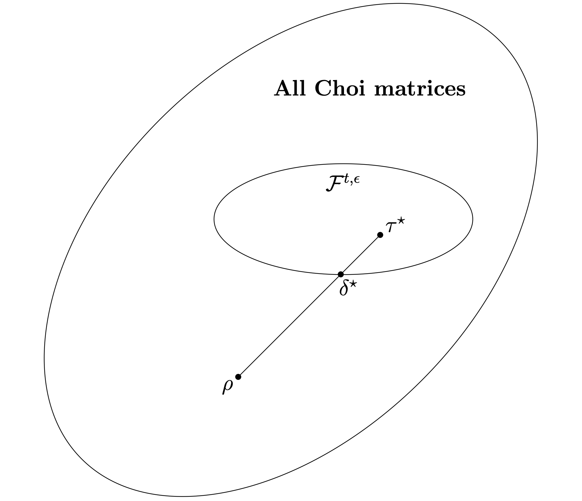
Figure 1: Geometrical interpretation of the robustness of non-Markovianity for a Choi matrix $\rho$. The outer ellipse is the (convex) set of all Choi matrices and $\mathcal{F}^{t,\epsilon}$ is the (convex) set of Markovian Choi matrices. The $\tau^{\star},\delta^{\star}$ correspond to the optimal decomposition.

III Properties of RoNM

Faithfulness.—Faithfulness follows directly from the definition. If $\Lambda\in\mathcal{O}_{\mathcal{F}}$, then clearly $\mathcal{N}_{\mathcal{R}}(\Lambda)=0$, since we do not need to mix any amount of Markovian noise to make it Markovian. Conversely, $\mathcal{N}_{\mathcal{R}}(\Lambda)=0\implies\Lambda\in\mathcal{O}_{\mathcal{F}}$.

Convexity.—Given two Choi matrices $\rho_{1}$ and $\rho_{2}$ with optimal decompositions (see main text, Eq. (5)), we have $\rho_{k}=\left(1+\mathcal{N}_{\mathcal{R}}(\rho_{k})\right)\delta_{k}^{\star}-\mathcal{N}_{\mathcal{R}}(\rho_{k})\tau^{\star}_{k}$, where $k=1,2$. Then, a convex combination of these two matrices, $\rho=p\rho_{1}+\left(1-p\right)\rho_{2}$, with $0\leq p\leq 1$ can be written as $\rho=\left(1+s\right)\delta-s\tau$, by choosing

$$\delta =\frac{p\left(1+\mathcal{N}_{\mathcal{R}}(\rho_{1})\right)\delta_{1}^{\star}+\left(1-p\right)\left(1+\mathcal{N}_{\mathcal{R}}(\rho_{2})\right)\delta_{2}^{\star}}{\left(1+s\right)}\in\mathcal{F},$$

$$\tau =\frac{p\mathcal{N}_{\mathcal{R}}(\rho_{1})\tau_{1}^{\star}+\left(1-p\right)\mathcal{N}_{\mathcal{R}}(\rho_{2})\tau_{2}^{\star}}{s}\in\mathcal{F},\text{ and}$$

$$s =p\mathcal{N}_{\mathcal{R}}(\rho_{1})+\left(1-p\right)\mathcal{N}_{\mathcal{R}}(\rho_{2}).$$

And since $\mathcal{N}_{\mathcal{R}}(\rho)\leq s$, we have

$$\mathcal{N}_{\mathcal{R}}\left(p\rho_{1}+\left(1-p\right)\rho_{2}\right)\leq p\mathcal{N}_{\mathcal{R}}(\rho_{1})+\left(1-p\right)\mathcal{N}_{\mathcal{R}}(\rho_{2}).$$ (S9)

A similar proof follows for the robustness of the map corresponding to the Choi matrix $\rho_{\Lambda}$.

Monotonicity under free operations.—The free operations in this setting are the Markovian maps, which are quantum channels or completely positive trace-preserving (CPTP) maps. Consider the composition of a non-Markovian map, say, $\Lambda$, with a free operation, say $\Gamma$, i.e., $\Gamma\circ\Lambda\equiv\Gamma\left(\Lambda\right)$. Then, using the closed form expression for $\mathcal{N}_{\mathcal{R}}(\Lambda)$ in terms of its corresponding Choi matrix $\rho_{\Lambda}$ (see Section VII), we have,

$$\mathcal{N}_{\mathcal{R}}(\Gamma\circ\Lambda)=\frac{\mathinner{\!\left\lVert\rho_{\left(\Gamma\circ\Lambda\right)}\right\rVert}_{1}-1}{2},$$

$$=\frac{\mathinner{\!\left\lVert\left(\mathbb{I}\otimes\Gamma\right)\left\{\mathbb{I}\otimes\Lambda\left(|\Phi^{+}\rangle\langle\Phi^{+}|\right)\right\}\right\rVert}_{1}-1}{2},$$

$$=\frac{\mathinner{\!\left\lVert\left(\mathbb{I}\otimes\Gamma\right)\rho_{\Lambda}\right\rVert}_{1}-1}{2},$$

$$\leq\frac{\mathinner{\!\left\lVert\rho_{\Lambda}\right\rVert}_{1}-1}{2}=\mathcal{N}_{\mathcal{R}}(\Lambda),$$

where in the last inequality, we’ve used the fact that if $\Lambda$ is a quantum channel and $\Delta\in\mathcal{B}(\mathcal{H}\otimes\mathcal{H})$ is Hermitian, then, $\mathinner{\!\left\lVert\left(\mathbb{I}\otimes\Lambda\right)(\Delta)\right\rVert}_{1}\leq\mathinner{\!\left\lVert\Delta\right\rVert}_{1}$ (see Eq. S5). Therefore, the RoNM measure is monotonic under composition with free operations. Together, these imply that the RoNM is a faithful, convex, and monotonic measure of quantum non-Markovianity.

IV RoNM as advantage in state discrimination

Given an ensemble of quantum states, $\mathcal{E}=\left\{p_{j},\sigma_{j}\right\}_{j}$ and a map $\mathbb{I}\otimes\Lambda$, we are to distinguish which state $\sigma_{j}$ has been selected from the ensemble by a single application of the map followed by a measurement with positive operator-valued measure (POVM) elements $\mathbb{M}=\left\{M_{j}\right\}_{j},\text{ s.t. }M_{j}\geq 0,\sum_{j}M_{j}=\mathbb{I}$. The average success probability for this task is $p_{\mathrm{succ}}\left(\mathcal{E},\mathbb{M},\mathbb{I}\otimes\Lambda\right)=\sum_{j}p_{j}\operatorname{Tr}\left[\mathbb{I}\otimes\Lambda\left(\sigma_{j}\right)M_{j}\right]$. Then, we have the following theorem.

Remark.—For ease of understanding, we make the ensemble, $\mathcal{E}=\left\{p_{j},\sigma_{j}\right\}_{j}$ and the POVM, $\mathbb{M}=\left\{M_{j}\right\}_{j},\text{ s.t. }M_{j}\geq 0,\sum_{j}M_{j}=\mathbb{I}$ explicit in the theorem below.

Theorem 6 (main text).

For any map $\Lambda$, Markovian or non-Markovian, we have,

$$\max_{\mathcal{E},\mathbb{M}}\frac{p_{\mathrm{succ}}\left(\mathcal{E},\mathbb{M},\mathrm{I}\otimes\Lambda\right)}{\max\limits_{\Gamma\in\mathcal{O}_{\mathcal{F}}}p_{\mathrm{succ}}\left(\mathcal{E},\mathbb{M},\mathbb{I}\otimes\Gamma\right)}=1+\mathcal{N}_{\mathcal{R}}(\Lambda).$$

Proof.

Consider the optimal decomposition of $\Lambda$,

$$\Lambda=\left(1+s^{\star}\right)\Gamma-s^{\star}\Phi,$$

where $s^{\star}=\mathcal{N}_{\mathcal{R}}(\Lambda)$, and $\Gamma,\Phi\in\mathcal{O}_{\mathcal{F}}$. Then, the average success probability is

$$\sum\limits_{j}p_{j}\operatorname{Tr}\left[\mathrm{I}\otimes\Lambda\left(\sigma_{j}\right)M_{j}\right]=\sum\limits_{j}p_{j}\left(1+s^{\star}\right)\operatorname{Tr}\left[\mathrm{I}\otimes\Gamma\left(\sigma_{j}\right)M_{j}\right]-\underbrace{\sum\limits_{j}p_{j}s^{\star}\operatorname{Tr}\left[\mathrm{I}\otimes\Phi\left(\sigma_{j}\right)M_{j}\right]}_{\geq 0}$$ (S10)

$$\leq\sum\limits_{j}p_{j}\left(1+s^{\star}\right)\operatorname{Tr}\left[\mathrm{I}\otimes\Gamma\left(\sigma_{j}\right)M_{j}\right]\leq\left(1+s^{\star}\right)\max_{\Gamma\in\mathcal{O}_{\mathcal{F}}}p_{\mathrm{succ}}\left(\left\{p_{j},\sigma_{j}\right\},\left\{M_{j}\right\},\mathrm{I}\otimes\Gamma\right),$$

where $s^{\star}=\mathcal{N}_{\mathcal{R}}(\Lambda)$. In Eq. S10, the under-braced term is non-negative, since in our definition of the RoNM we choose $\Phi\in\mathcal{O}_{\mathcal{F}}$. However, if we were to define a “generalized” robustness measure (in the sense of mixing w.r.t all maps), this would not hold true. Therefore, we have that

$$\frac{p_{\mathrm{succ}}\left(\left\{p_{j},\sigma_{j}\right\},\left\{M_{j}\right\},\mathrm{I}\otimes\Lambda\right)}{\max\limits_{\Gamma\in O_{\mathcal{F}}}p_{\mathrm{succ}}\left(\left\{p_{j},\sigma_{j}\right\},\left\{M_{j}\right\},\mathbb{I}\otimes\Gamma\right)}\leq 1+\mathcal{N}_{\mathcal{R}}(\Lambda).$$ (S11)

Then, by maximizing over all ensembles, $\left\{p_{j},\sigma_{j}\right\}$ and all POVMs, $\{M_{j}\}$, we have that the LHS is $\leq 1+\mathcal{N}_{\mathcal{R}}(\Lambda)$.

We now prove the converse part of the theorem. Recall that for a POVM element to form a valid measurement, we must have $M_{j}\leq\mathbb{I}\,\forall j$. Then, $\mathinner{\!\left\lVert M_{j}\right\rVert}_{\infty}\leq 1$. Therefore, we consider a specific measurement

$$\left\{\frac{X}{\|X\|_{\infty}},\mathbb{I}-\frac{X}{\|X\|_{\infty}}\right\},$$

where $X$ is an optimal solution of the dual SDP (see main text, Eq. (12)), and the ensemble $\{p_{j},\sigma_{j}\}_{j=0}^{1}$, with $p_{0}=1,\sigma_{0}=|\Phi^{+}\rangle\langle\Phi^{+}|$, where $|\Phi^{+}\rangle$ is the (normalized) maximally entangled state, and $p_{1}=0$ and $\sigma_{1}$ is some arbitrary state. For this choice, we then have

$$\frac{p_{\mathrm{succ}}\left(\left\{p_{j},\sigma_{j}\right\},\left\{M_{j}\right\},\mathbb{I}\otimes\Lambda\right)}{\max\limits_{\Gamma_{j}\in O_{\mathcal{F}}}p_{\mathrm{succ}}\left(\left\{p_{j},\sigma_{j}\right\},\left\{M_{j}\right\},\mathbb{I}\otimes\Gamma\right)}$$

$$=\frac{\operatorname{Tr}\left[\mathbb{I}\otimes\Lambda(|\Phi^{+}\rangle\langle\Phi^{+}|\right)X]}{\max\limits_{\Gamma\in O_{\mathcal{F}}}\operatorname{Tr}\left[\mathbb{I}\otimes\Gamma\left(\left|\Phi^{+}\rangle\langle\Phi^{+}\right|\right)X\right]},$$

$$=\frac{\text{Tr}\left[\rho_{\Lambda}X\right]}{\max\limits_{\Gamma\in\mathcal{O}_{\mathcal{F}}}\text{Tr}\left[\rho_{\Gamma}X\right]}\geq\left(1+\mathcal{N}_{\mathcal{R}}(\Lambda)\right),$$ (S12)

where the last inequality follows from the dual SDP formulation.

We now have both an upper and a lower bound. From the first half of the proof, we have that the LHS of Theorem 2 (main text) is $\leq\left(1+\mathcal{N}_{\mathcal{R}}(\Lambda)\right)$. Since the LHS is (already) maximized over all measurements and ensembles, in particular, it is greater than or equal to the value for the particular ensemble and measurements chosen above (since it is the maximum). On the other hand, using the converse part of the proof (as shown by Section IV), we have that the LHS is $\geq\left(1+\mathcal{N}_{\mathcal{R}}(\Lambda)\right)$. Therefore, combining these two, it must be equal to the RHS, which completes the proof. ∎

V RoNM as advantage in channel discrimination

Suppose we have access to an ensemble of maps, i.e., a quantum operation sampled from the prior distribution, $\mathcal{E}_{\Lambda}=\left\{p_{j},\Lambda_{j}\right\}_{j=0}^{N-1}$. We apply one map chosen at random from this ensemble to one subsystem of a bipartite state $\Psi\in\mathcal{D}\left(\mathcal{H}\otimes\mathcal{H}\right)$, and perform a collective measurement on the output system by measurement operators $\mathbb{M}=\left\{M_{j}\right\}_{j=0}^{N}$. We also allow measurements with inconclusive outcomes; for example, when using POVMs to distinguish non-orthogonal states. Then, the average success probability for this task is $\widetilde{p}_{\mathrm{succ}}\left(\mathcal{E}_{\Lambda},\mathbb{M},\Psi\right)=\sum_{j=0}^{N-1}p_{j}\operatorname{Tr}\left[\left\{\mathbb{I}\otimes\Lambda_{j}(\Psi)\right\}M_{j}\right]$, where inconclusive measurement outcomes do not contribute to the success probability. For the ensemble of maps, we also define $\widetilde{\mathcal{N}}_{\mathcal{R}}\left(\mathcal{E}_{\Lambda}\right)\equiv\max_{j}\mathcal{N}_{\mathcal{R}}\left(\Lambda_{j}\right)$. Then, we can connect the maximal advantage in this channel discrimination task to the maximum robustness of the ensemble of maps.

Theorem 7 (main text).

For an ensemble of maps, $\mathcal{E}_{\Lambda}$ as defined above, we have,

$$\max\limits_{\Psi,\mathbb{M}}\frac{\widetilde{p}_{\mathrm{succ}}\left(\mathcal{E}_{\Lambda},\mathbb{M},\Psi\right)}{\max\limits_{\Gamma\in O_{\mathcal{F}}}\widetilde{p}_{\mathrm{succ}}\left(\mathcal{E}_{\Gamma},\mathbb{M},\Psi\right)}=1+\widetilde{\mathcal{N}}_{\mathcal{R}}\left(\mathcal{E}_{\Lambda}\right),$$

where $\Psi\in\mathcal{D}\left(\mathcal{H}\otimes\mathcal{H}\right)$ is the set of all bipartite density matrices.

Proof.

Similar to the proof for the state discrimination game, we have,

$$\widetilde{p}_{\mathrm{succ}}\left(\left\{p_{j},\mathbb{I}\otimes\Lambda_{j}\right\}_{j=0}^{N-1},\left\{M_{j}\right\}_{j=0}^{N},\Psi\right)$$

$$=\sum_{j=0}^{N-1}p_{j}\operatorname{Tr}\left[\left\{\mathbb{I}\otimes\Lambda_{j}(\Psi)\right\}M_{j}\right]$$

$$\leq\sum_{j=0}^{N-1}p_{j}\left(1+r_{j}\right)\operatorname{Tr}\left[\left\{\mathbb{I}\otimes\Gamma_{j}(\Psi)\right\}M_{j}\right]$$

$$\leq\left(1+r_{j^{\star}}\right)\max_{\Gamma_{j}\in O_{\mathcal{F}}}\widetilde{p}_{\mathrm{succ}}\left(\left\{p_{j},\mathbb{I}\otimes\Gamma_{j}\right\}_{j=0}^{N-1},\left\{M_{j}\right\}_{j=0}^{N},\Psi\right),$$

where $r_{j}\mathrel{\mathop{\mathchar 58\relax}}=\mathcal{N}_{\mathcal{R}}(\Lambda_{j})$ and $j^{\star}=\text{argmax}_{j}r_{j}$. Once again, note that the choice of $\Phi\in\mathcal{O}_{\mathcal{F}}$ is crucial in the inequality above.

To prove the converse part of the theorem, we proceed in a similar fashion as before and make a specific choice of ensemble and POVMs. Consider, $\Psi=|\Phi^{+}\rangle\langle\Phi^{+}|$, and the POVM, $M_{j^{\star}}=X_{j^{\star}}/\mathinner{\!\left\lVert X_{j}^{\star}\right\rVert}_{\infty}$, where $X_{j^{\star}}$ is an optimal witness from the dual SDP formulation for $\Lambda_{j^{\star}}$ (see main text, Eq. (12)). Define, $M_{j}=0$ for $j\neq j^{\star}$ and $M_{N}=\mathbb{I}-M_{j^{\star}}$. Then, for this specific choice of the state and measurements, we have

$$\frac{\widetilde{p}_{\mathrm{succ}}\left(\left\{p_{j},\mathbb{I}\otimes\Lambda_{j}\right\}_{j=0}^{N-1},\left\{M_{j}\right\}_{j=0}^{N},\Psi\right)}{\max\limits_{\Gamma_{j}\in O_{\mathcal{F}}}\widetilde{p}_{\mathrm{succ}}\left(\left\{p_{j},\mathbb{I}\otimes\Gamma_{j}\right\}_{j=0}^{N-1},\left\{M_{j}\right\}_{j=0}^{N},\Psi\right)},$$

$$=\frac{\sum\limits_{j=0}^{N-1}p_{j}\operatorname{Tr}\left[\left\{\mathbb{I}\otimes\Lambda_{j}\left(\left|\Phi^{+}\rangle\langle\Phi^{+}\right|\right)\right\}M_{j}\right]}{\max\limits_{\Gamma_{j}\in O_{\mathcal{F}}}\sum\limits_{j=0}^{N-1}p_{j}\operatorname{Tr}\left[\left\{\mathbb{I}\otimes\Gamma_{j}(|\Phi^{+}\rangle\langle\Phi^{+}|\right)\}M_{j}\right]},$$

$$=\frac{p_{j^{\star}}\operatorname{Tr}\left[\rho_{\Lambda_{j}\star}X_{j^{\star}}\right]}{\max\limits_{\Gamma\in O_{\mathcal{F}}}p_{j^{\star}}\operatorname{Tr}\left[\rho_{\Gamma}X_{j^{\star}}\right]},$$

$$\leq 1+\widetilde{\mathcal{N}}_{\mathcal{R}}(\left\{p_{j},\Lambda_{j}\right\}),$$ (S13)

where the last inequality is due to the dual SDP formulation. Then, by combining the converse part of the proof with the first half, the proof is complete by a similar argument as in the previous theorem. ∎

VI Connection to single-shot information theory

The single-shot variant of the accessible information for a channel is defined as

$$I_{\min}^{\mathrm{acc}}(\Lambda)\equiv\max_{\mathcal{E},\mathbb{M}}\leavevmode\nobreak\ I_{\min}(X;Y),$$ (S14)

where $I_{\text{min}}(X;Y)\equiv H_{\text{min}}(X)-H_{\text{min}}(X|Y)$, and $H_{\text{min}}(X)=-\log\left(\max_{x}p(x)\right)$, $H_{\text{min}}(X|Y)=-\log(\sum\limits_{y}\max_{x}p(x,y))$ are the min-entropy and min-conditional entropy, respectively (see also Ref. Skrzypczyk and Linden (2019)).

Theorem 8 (main text).

For any map $\Lambda$, Markovian or non-Markovian, we have,

$$I^{\mathrm{acc}}_{\mathrm{min}}(\Lambda)-\max_{\Gamma\in\mathcal{O}_{\mathcal{F}}}I^{\mathrm{acc}}_{\mathrm{min}}(\Gamma)\leq\log\left(1+\mathcal{N}_{\mathcal{R}}(\Lambda)\right).$$

Proof.

Consider a non-Markovian map, $\Lambda$, with the optimal decomposition, $\Lambda=(1+s)\Gamma-s\Phi,\text{ where }s=\mathcal{N}_{\mathcal{R}}(\Lambda)$, then,

$$I^{\text{acc}}_{\text{min}}(\Lambda)=\max_{\{\sigma_{j},p_{j},N_{y}\}}I_{\text{min}}(X;Y;\Lambda)$$

$$=\max_{\{\sigma_{j},p_{j},N_{y}\}}\log\left(\frac{\sum\limits_{y}\max_{j}p(j)\text{Tr}\left[\Lambda(\sigma_{j})N_{y}\right]}{p_{\text{max}}}\right)$$

Then, plugging in the optimal decomposition, we have

$$=\max_{\{\sigma_{j},p_{j},N_{y}\}}\log\left(\frac{\sum\limits_{y}\max_{j}p(j)\text{Tr}\left[\left((1+s)\Gamma(\sigma_{j})-s\Phi(\sigma_{j})\right)N_{y}\right]}{p_{\text{max}}}\right)$$

$$=\max_{\{\sigma_{j},p_{j},N_{y}\}}\log\left((1+s)\frac{\sum\limits_{y}\max_{j}p(j)\text{Tr}\left[\Gamma(\sigma_{j})N_{y}\right]}{p_{\text{max}}}-\underbrace{s\frac{\sum\limits_{y}\max_{j}p(j)\text{Tr}\left[\Phi(\sigma_{j})N_{y}\right]}{p_{\text{max}}}}_{\geq 0}\right).$$

Since, $\log(\cdot)$ is monotonic, we have, $\log\left(a-b\right)\leq\log\left(a\right),\text{ if }b\geq 0$. Therefore,

$$\leq\max_{\{\sigma_{j},p_{j},N_{y}\}}\log\left((1+s)\frac{\sum\limits_{y}\max_{j}p(j)\text{Tr}\left[\Gamma(\sigma_{j})N_{y}\right]}{p_{\text{max}}}\right)$$

Now we can maximize over all Markovian maps $\Gamma$, to get

$$\leq\max_{\Gamma\in\mathcal{O}_{\mathcal{F}}}\max_{\{\sigma_{j},p_{j},N_{y}\}}\log\left((1+s)\frac{\sum\limits_{y}\max_{j}p(j)\text{Tr}\left[\Gamma(\sigma_{j})N_{y}\right]}{p_{\text{max}}}\right)$$

By using $\log\left(a\times b\right)=\log\left(a\right)+\log\left(b\right)$, we have

$$\leq\max_{\Gamma\in\mathcal{O}_{\mathcal{F}}}\max_{\{\sigma_{j},p_{j},N_{y}\}}\log\left(\frac{\sum\limits_{y}\max_{j}p(j)\text{Tr}\left[\Gamma(\sigma_{j})N_{y}\right]}{p_{\text{max}}}\right)$$

$$+\log\left(1+\mathcal{N}_{\mathcal{R}}(\Lambda)\right).$$

Therefore,

$$I^{\text{acc}}_{\text{min}}(\Lambda)-\max_{\Gamma\in\mathcal{O}_{\mathcal{F}}}I^{\text{acc}}_{\text{min}}(\Gamma)\leq\log\left(1+\mathcal{N}_{\mathcal{R}}(\Lambda)\right).$$

∎

VII Relating the RoNM to the RHP measure

We now relate the RoNM to the RHP measure. This relation, in turn, provides an operational meaning to the RHP measure. Consider the optimal decomposition for a Choi matrix:

$$\rho=\left(1+s^{\star}\right)\delta-s^{\star}\tau,\text{ where }s^{\star}=\mathcal{N}_{\mathcal{R}}(\rho)\text{ and }\tau,\delta\geq 0.$$

The spectral decomposition of $\rho$ can be written

$$\rho=\Delta^{+}-\Delta^{-},\text{ where }\Delta^{\pm}\geq 0.$$

Comparing the two decompositions, we see that $\Delta^{-}=s^{\star}\tau\implies\mathinner{\!\left\lVert\Delta^{-}\right\rVert}_{1}=s^{\star}=\mathcal{N}_{\mathcal{R}}(\rho)$, since $\mathinner{\!\left\lVert\tau\right\rVert}_{1}=1$. Also,

$$\mathinner{\!\left\lVert\rho\right\rVert}_{1}=\mathinner{\!\left\lVert\Delta^{+}\right\rVert}_{1}+\mathinner{\!\left\lVert\Delta^{-}\right\rVert}_{1}=\text{Tr}\left[\Delta^{+}\right]+\text{Tr}\left[\Delta^{-}\right].$$ (S15)

Since the map $\Lambda$ corresponding to the Choi matrix $\rho$ is trace-preserving, we have

$$\text{Tr}\left[\rho\right]=\text{Tr}\left[\Delta^{+}\right]-\text{Tr}\left[\Delta^{-}\right]=1.$$ (S16)

Subtracting Eq. S16 from Eq. S15, we have

$$\mathinner{\!\left\lVert\rho\right\rVert}_{1}-1 =2\text{Tr}\left[\Delta^{-}\right]=2\mathinner{\!\left\lVert\Delta^{-}\right\rVert}_{1}=2\mathcal{N}_{\mathcal{R}}(\rho)$$

$$\implies\mathcal{N}_{\mathcal{R}}(\rho) =\frac{\mathinner{\!\left\lVert\rho\right\rVert}_{1}-1}{2}.$$ (S17)

Now, recall that the RHP measure for some evolution $\Lambda$ is defined as (see page 3 of Ref. Rivas et al. (2010))

$$\mathcal{I}=\int_{0}^{\infty}dt\lim_{\epsilon\rightarrow 0^{+}}\frac{\left(f_{\mathrm{NCP}}(t+\epsilon,t)-1\right)}{\epsilon},$$ (S18)

where $f_{\mathrm{NCP}}(t+\epsilon,t)\mathrel{\mathop{\mathchar 58\relax}}=\|(\Lambda_{(t+\epsilon,t)}\otimes\mathbb{I})(|\Phi\rangle\langle\Phi|)\|_{1}=\mathinner{\!\left\lVert\rho_{\Lambda}\right\rVert}_{1}$.

Before comparing the RHP and RoNM, we note that, by construction, $\rho$ is a function of both $t$ and $\epsilon$. Therefore, we’ll need to remove the $\epsilon$ dependence and integrate over all time; where the only contribution comes from the times at which the map (and hence the measure) is non-Markovian. That is, define

$$\mathcal{N}^{\text{total}}_{\mathcal{R}}(\rho)\equiv\int\limits_{0}^{\infty}dt\lim_{\epsilon\rightarrow 0^{+}}\left(\frac{\mathcal{N}_{\mathcal{R}}(\rho)}{\epsilon}\right).$$

Comparing to the RHP measure, we have

$$\mathcal{N}^{\text{total}}_{\mathcal{R}}(\rho) =\int\limits_{0}^{\infty}dt\lim_{\epsilon\rightarrow 0^{+}}\left(\frac{\mathcal{N}_{\mathcal{R}}(\rho)}{\epsilon}\right)$$

$$=\frac{1}{2}\int\limits_{0}^{\infty}dt\lim_{\epsilon\rightarrow 0^{+}}\left(\frac{\mathinner{\!\left\lVert\rho\right\rVert}_{1}-1}{\epsilon}\right)$$

$$=\frac{1}{2}\int_{0}^{\infty}dt\lim_{\epsilon\rightarrow 0^{+}}\frac{\left(f_{\mathrm{NCP}}(t+\epsilon,t)-1\right)}{\epsilon}$$

$$=\frac{\mathcal{I}}{2}.$$ (S19)

Therefore, the RoNM and the RHP measure are equal upto a factor of one-half.

Moreover, one can also define a normalized version of the measure (in analogy to the normalized measure of RHP),

$$\mathcal{N}^{\text{norm}}_{\mathcal{R}}\mathrel{\mathop{\mathchar 58\relax}}=\mathcal{N}^{\text{total}}_{\mathcal{R}}/\left(1+\mathcal{N}^{\text{total}}_{\mathcal{R}}\right),$$ (S20)

such that, $\mathcal{N}^{\text{norm}}_{\mathcal{R}}=0$ for $\mathcal{N}^{\text{total}}_{\mathcal{R}}=0$ (Markovian evolution) and $\mathcal{N}^{\text{norm}}_{\mathcal{R}}\rightarrow 1$ for $\mathcal{N}^{\text{total}}_{\mathcal{R}}\rightarrow\infty$.

VIII Analytical form for single qubit-channels

We now consider a single-qubit dephasing channel as an analytical example. The Lindblad equation for this channel has the form:

$$\frac{d\rho}{dt}=\gamma(t)\left(\sigma_{z}\rho\sigma_{z}-\rho\right),$$ (S21)

where $\gamma(t)$ is the rate of dephasing. In the small time approximation, the eigenvalues of the Choi matrix are $\{0,0,\epsilon\gamma(t),1-\epsilon\gamma(t)\}$, respectively. For Markovian operations, $\gamma(t)\geq 0$, but for non-Markovian operations $\gamma(t)$ can be negative. Note that for small $\epsilon$, if the rate is negative then all the eigenvalues of $\rho$ are positive except for $\epsilon\gamma(t)$. Then, we have Rivas et al. (2010)

$$g(t)=\left\{\begin{array}[]{ l l }{0}&{\gamma(t)\geq 0,}\\ {-2\gamma(t)}&{\gamma(t)<0,}\end{array}\right.$$ (S24)

and

$$\lim_{\epsilon\rightarrow 0^{+}}\left(\frac{\mathcal{N}_{\mathcal{R}}(\rho)}{\epsilon}\right)=\left\{\begin{array}[]{ l l }{0}&{\gamma(t)\geq 0,}\\ {-\gamma(t)}&{\gamma(t)<0.}\end{array}\right..$$ (S27)

As a result, $\mathcal{N}_{\mathcal{R}}^{\text{ total }}=\mathcal{I}/2$, for the dephasing channel, where $\mathcal{I}$ is the RHP measure.

References

- Breuer and Petruccione (2002) H.-P. Breuer and F. Petruccione, The Theory of Open Quantum Systems (Oxford University Press, Oxford ; New York, 2002) oCLC: ocm49872077.
- Rivas and Huelga (2012) A. Rivas and S. F. Huelga, Open Quantum Systems an Introduction (Springer Berlin Heidelberg, Berlin, Heidelberg, 2012) oCLC: 939917111.
- Rivas et al. (2014) A. Rivas, S. F. Huelga, and M. B. Plenio, Reports on Progress in Physics 77, 094001 (2014).
- Breuer et al. (2016) H.-P. Breuer, E.-M. Laine, J. Piilo, and B. Vacchini, Reviews of Modern Physics 88 (2016), 10.1103/RevModPhys.88.021002.
- Alicki and Lendi (2007) R. Alicki and K. Lendi, Quantum Dynamical Semigroups and Applications, Lecture Notes in Physics No. 717 (Springer-Verlag, Berlin ; New York, 2007).
- Breuer et al. (2009) H.-P. Breuer, E.-M. Laine, and J. Piilo, Physical Review Letters 103 (2009), 10.1103/PhysRevLett.103.210401.
- Rivas et al. (2010) A. Rivas, S. F. Huelga, and M. B. Plenio, Physical Review Letters 105 (2010), 10.1103/PhysRevLett.105.050403.
- Wolf and Cirac (2008) M. M. Wolf and J. I. Cirac, Communications in Mathematical Physics 279, 147 (2008).
- Kossakowski (1972) A. Kossakowski, Reports on Mathematical Physics 3, 247 (1972).
- Lindblad (1976) G. Lindblad, Communications in Mathematical Physics 48, 119 (1976).
- Gorini et al. (1976) V. Gorini, A. Kossakowski, and E. C. G. Sudarshan, Journal of Mathematical Physics 17, 821 (1976).
- Laine et al. (2015) E.-M. Laine, H.-P. Breuer, and J. Piilo, Scientific Reports 4 (2015), 10.1038/srep04620.
- Thomas et al. (2018) G. Thomas, N. Siddharth, S. Banerjee, and S. Ghosh, Physical Review E 97 (2018), 10.1103/PhysRevE.97.062108.
- Addis et al. (2015) C. Addis, F. Ciccarello, M. Cascio, G. M. Palma, and S. Maniscalco, New Journal of Physics 17, 123004 (2015).
- Mirkin et al. (2019) N. Mirkin, P. Poggi, and D. Wisniacki, arXiv e-prints , arXiv:1903.07489 (2019), arXiv:1903.07489 [quant-ph] .
- Chitambar and Gour (2019) E. Chitambar and G. Gour, Rev. Mod. Phys. 91, 025001 (2019).
- Plenio and Virmani (2005) M. B. Plenio and S. Virmani, arXiv:quant-ph/0504163 (2005), arXiv:quant-ph/0504163 .
- Aberg (2006) J. Aberg, arXiv:quant-ph/0612146 (2006), arXiv:quant-ph/0612146 .
- Baumgratz et al. (2014) T. Baumgratz, M. Cramer, and M. B. Plenio, Physical Review Letters 113 (2014), 10.1103/PhysRevLett.113.140401.
- Streltsov et al. (2017) A. Streltsov, G. Adesso, and M. B. Plenio, Reviews of Modern Physics 89 (2017), 10.1103/RevModPhys.89.041003.
- Napoli et al. (2016) C. Napoli, T. R. Bromley, M. Cianciaruso, M. Piani, N. Johnston, and G. Adesso, Physical Review Letters 116 (2016), 10.1103/PhysRevLett.116.150502.
- Takagi et al. (2019) R. Takagi, B. Regula, K. Bu, Z.-W. Liu, and G. Adesso, Phys. Rev. Lett. 122, 140402 (2019).
- Takagi and Regula (2019) R. Takagi and B. Regula, arXiv:1901.08127 [quant-ph] (2019), arXiv:1901.08127 [quant-ph] .
- Skrzypczyk and Linden (2019) P. Skrzypczyk and N. Linden, Phys. Rev. Lett. 122, 140403 (2019).
- Uola et al. (2019) R. Uola, T. Kraft, J. Shang, X.-D. Yu, and O. Gühne, Phys. Rev. Lett. 122, 130404 (2019).
- Note (1) In Refs. Bhattacharya et al. (2018); Bhattacharya and Bhattacharya (2018), the authors construct a resource theory for non-Markovianity where they identify the set of free states as the Choi-Jamałkowski matrices corresponding to Markovian maps. Although this construction is in some ways easier to work with, since there are both designated free states and free operations, this quickly leads into difficulties. Any resourceful operation can transform a free state (a Choi matrix for a Markovian map, which is normalized and positive semidefinite) into a non-state (since it can now have negative eigenvalues) and so it can take us outside the set of quantum states, which is usually assumed to be the landscape for quantum resource theories. To circumvent such obstacles, we avoid such an identification and only define a set of free operations.
- Chiribella et al. (2008) G. Chiribella, G. M. D’Ariano, and P. Perinotti, EPL (Europhysics Letters) 83, 30004 (2008), arXiv:0804.0180 [quant-ph] .
- Choi (1975) M.-D. Choi, Linear Algebra and its Applications 10, 285 (1975).
- Jamiołkowski (1972) A. Jamiołkowski, Reports on Mathematical Physics 3, 275 (1972).
- Bhattacharya et al. (2018) S. Bhattacharya, B. Bhattacharya, and A. S. Majumdar, arXiv:1803.06881 [quant-ph] (2018), arXiv:1803.06881 [quant-ph] .
- Note (2) The name generalized robustness is slightly unfortunate for this context. Generalized robustness is defined as mixing with respect to the set of all CPTP maps, which is usually also the most general set with which mixing is possible. However, when considering non-Markovian maps, which lie outside the set of CPTP maps, the robustness measure defined via the most general form of mixing (using both Markovian and non-Markovian maps) is not termed the generalized robustness.
- Boyd and Vandenberghe (2004) S. P. Boyd and L. Vandenberghe, Convex Optimization (Cambridge University Press, Cambridge, UK ; New York, 2004).
- Watrous (2018) J. Watrous, The Theory of Quantum Information, 1st ed. (Cambridge University Press, 2018).
- Bae and Chruściński (2016) J. Bae and D. Chruściński, Phys. Rev. Lett. 117, 050403 (2016).
- Wilde (2017) M. M. Wilde, “Preface to the second edition,” in Quantum Information Theory (Cambridge University Press, 2017) pp. xi–xii, 2nd ed.
- Ciganović et al. (2014) N. Ciganović, N. J. Beaudry, and R. Renner, IEEE Transactions on Information Theory 60, 1573 (2014).
- Fanchini et al. (2014) F. F. Fanchini, G. Karpat, B. Çakmak, L. K. Castelano, G. H. Aguilar, O. J. Farías, S. P. Walborn, P. H. S. Ribeiro, and M. C. de Oliveira, Phys. Rev. Lett. 112, 210402 (2014).
- Regula (2018) B. Regula, Journal of Physics A: Mathematical and Theoretical 51, 045303 (2018).
- Lu et al. (2010) X.-M. Lu, X. Wang, and C. P. Sun, Phys. Rev. A 82, 042103 (2010).
- Chruściński and Maniscalco (2014) D. Chruściński and S. Maniscalco, Phys. Rev. Lett. 112, 120404 (2014).
- He et al. (2017) Z. He, H.-S. Zeng, Y. Li, Q. Wang, and C. Yao, Phys. Rev. A 96, 022106 (2017).
- Dhar et al. (2015) H. S. Dhar, M. N. Bera, and G. Adesso, Physical Review A 91 (2015), 10.1103/PhysRevA.91.032115.
- Chancellor et al. (2014) N. Chancellor, C. Petri, L. Campos Venuti, A. F. J. Levi, and S. Haas, Phys. Rev. A 89, 052119 (2014).
- Bhattacharya and Bhattacharya (2018) B. Bhattacharya and S. Bhattacharya, arXiv:1805.11418 [quant-ph] (2018), arXiv:1805.11418 [quant-ph] .
Supplemental Material for “Quantifying non-Markovianity: a quantum resource-theoretic approach”