The Type II-Plateau Supernova 2017eaw in NGC 6946 and Its Red Supergiant Progenitor

Abstract

We present extensive optical photometric and spectroscopic observations, from 4 to 482 days after explosion, of the Type II-plateau (II-P) supernova (SN) 2017eaw in NGC 6946. SN 2017eaw is a normal SN II-P intermediate in properties between, for example, SN 1999em and SN 2012aw and the more luminous SN 2004et, also in NGC 6946. We have determined that the extinction to SN 2017eaw is primarily due to the Galactic foreground and that the SN site metallicity is likely subsolar. We have also independently confirmed a tip-of-the-red-giant-branch (TRGB) distance to NGC 6946 of $7.73{\pm}0.78$ Mpc. The distances to the SN that we have also estimated via both the standardized candle method and expanding photosphere method corroborate the TRGB distance. We confirm the SN progenitor identity in pre-explosion archival Hubble Space Telescope (HST) and Spitzer Space Telescope images, via imaging of the SN through our HST Target of Opportunity program. Detailed modeling of the progenitor’s spectral energy distribution indicates that the star was a dusty, luminous red supergiant consistent with an initial mass of $\sim 15\ M_{\odot}$.

1 Introduction

Supernovae (SNe) have a profound influence on the host galaxies in which they occur: through chemical enrichment, galactic feedback, and the formation of compact neutron star and black hole remnants. A large fraction of SNe, $\sim 76$% in the local Universe (Li et al. 2011), arise from the core collapse of massive stars with initial masses $M_{\rm ini}\gtrsim 8$–$10\ M_{\odot}$. The most common of these core-collapse SNe are the Type II-Plateau (SNe II-P, $\sim 48$% locally; Smith et al. 2011).

Solid evidence has emerged through the direct identification of the progenitor stars of a number of recent, nearby SNe II-P that these explosions represent the termination of stars in the red supergiant (RSG) evolutionary phase (e.g., Van Dyk et al. 2003; Smartt et al. 2004; Maund & Smartt 2009; Van Dyk et al. 2012a; b; Fraser et al. 2012; 2014; Maund et al. 2014a; b). From a still incomplete sample of about 27 SNe II-P, it has been inferred that the initial mass range for RSGs leading to SNe II-P is $\sim 9.5$–$16.5\ M_{\odot}$ (Smartt et al. 2009; Smartt 2015). More indirect indicators, such as the ages of the immediate stellar environment (e.g., Williams et al. 2014; 2018; Maund 2017) and mass measurement of the nucleosynthetic products via modeling of SNe II-P nebular spectra (Jerkstrand et al. 2012; Jerkstrand et al. 2014), tend generally to agree with this approximate mass range. Corroborating evidence for the lack of SN II-P progenitors above an initial mass of $\sim 17\ M_{\odot}$, known as “the RSG problem,” stems from theoretical modeling of massive star explosions for which models at this approximate mass are unable to explode, but would instead collapse to form a black hole directly (e.g., Sukhbold et al. 2016). Related to this is the possible discovery of an RSG with $M_{\rm ini}\approx 22\ M_{\odot}$ which appears to have vanished, rather than terminated as an SN (Adams et al. 2017).

Several alternative possibilities have been offered to explain away the RSG problem, including enhanced wind-driven mass loss in more massive RSGs, stripping much of the H envelope (Yoon & Cantiello 2010; Georgy 2012); possible self-obscuration by more luminous, more massive RSGs possessing dustier envelopes (e.g., Walmswell & Eldridge 2012); and, inadequate assumptions of the bolometric correction for RSGs nearing explosion (Davies & Beasor 2018). In addition, Davies & Beasor (2018) have argued that the uncertainty in the mass-luminosity relationship, which can be different for various theoretical stellar evolution models, may shift the limiting mass up by as much as several solar masses. Furthermore, we note that some SN II-P/II-linear hybrid cases may have more massive progenitors (e.g., SN 2016X with $M_{\rm ini}\approx 19$–$20\ M_{\odot}$; Huang et al. 2018).

The mass function of SN II-P progenitors requires additional development through additional cases of directly identified progenitors. Furthermore, the data for existing examples are sparse, with initial progenitor masses being precariously inferred from fitting of a spectral energy distribution (SED) based on one or two photometric data points. Inevitably in the near future, the Large Synoptic Survey Telescope (LSST) and a possible general-observer program for nearby galaxies using the Wide-Field Infrared Survey Telescope (WFIRST) would provide detailed, multiband pre-explosion images for the progenitors of ever-larger numbers of discovered SNe II-P. In the meantime, we can continue to build the sample slowly through the smatterings of nearby SNe II-P for which sufficient archival ground- and space-based data are available.

To that end, in this paper we discuss the Type II-P SN 2017eaw, which was discovered by Wiggins (2017) at an unfiltered brightness of 12.8 mag on 2017 May 14.238 (UT dates are used throughout this paper). The discovery was confirmed by Dong & Stanek (2017). The object was found to be a young SN II-P by Cheng et al. (2017), Xiang et al. (2017), and Tomasella et al. (2017). A progenitor candidate was quickly identified by Khan (2017) in pre-explosion data obtained by the Spitzer Space Telescope and by Van Dyk et al. (2017) in archival Hubble Space Telescope (HST) data. Analyses of the progenitor have been published by Kilpatrick & Foley (2018) and Rui et al. (2019). Tsvetkov et al. (2018) presented detailed UBVRI light curves of the SN over the first 200 days. Rho et al. (2018) analyzed near-infrared spectroscopy of the SN to examine the possibility of dust formation. The dust properties of the evolving SN also have been explored by Tinyanont et al. (2019). SN 2017eaw is the tenth historical SN in the prodigious NGC 6946, also colloquially known as the “Fireworks Galaxy.” The other events are SN 1917A, SN 1939C, SN 1948B, SN 1968D (Hyman et al. 1995), SN 1969P, the Type II-L SN 1980K (e.g., Milisavljevic et al. 2012), the Type II-P SN 2002hh (e.g., Pozzo et al. 2006) and SN 2004et (e.g., Sahu et al. 2006; Maguire et al. 2010), and the “SN impostor” SN 2008S (Prieto et al. 2008; Botticella et al. 2009; Thompson et al. 2009). A number of SN remnants are also known to exist in this host galaxy (Matonick & Fesen 1997; Bruursema et al. 2014).

The organization of this paper is as follows. In Section 2 we describe the various observations of SN 2017eaw, both pre- and post-explosion. We estimate the extinction to the SN in Section 3, and in Section 4 we confirm recent estimates of the distance to the SN host galaxy. The metallicity at the SN site is inferred in Section 5. In Section 6 we provide an analysis of the SN, including an estimate of the date of explosion, studies of the absolute light curves, color curves, and bolometric light curve, an estimate of the synthesized nickel mass, and analysis of the spectra. In Section 7 we present identification and characterization of the SN progenitor. We provide a discussion and summarize our conclusions in Section 8.

2 Observations

2.1 SN Photometry

Multiband BVRI images of SN 2017eaw were obtained with both the Katzman Automatic Imaging Telescope (KAIT; Filippenko et al. 2001) and the 1 m Nickel telescope at Lick Observatory. Unfiltered images were also obtained with KAIT. All KAIT and Nickel images were reduced using a custom pipeline (Ganeshalingam et al. 2010).

We obtained near-daily BVRI coverage with the pt5m, a 0.5 m robotic telescope at the Roque de los Muchachos Observatory, La Palma (Hardy et al. 2015). Exposure times for these observations were $5\times 15$ s for both $B$ and $I$, and $5\times 10$ s for both $V$ and $R$, prior to 2017 October 26. From that date onward, exposure times were $5\times 45$ s for both $B$ and $I$, and $5\times 40$ s for both $V$ and $R$. All pt5m observations were reduced using bias, dark, and flat-field frames acquired on the same night (or as close in time as possible) as the science observations. Image alignment was conducted using astrometry.net, and coaddition of the images was performed using swarp (Bertin et al. 2002).

Calibration of the SN 2017eaw photometry was achieved via transformation from Pan-STARRS1 (PS1) magnitudes for stars in the field to BVRI, following relations provided by Tonry et al. (2012). We show the SN field with this local sequence of stars in Figure 1 and list their brightnesses in Table 1. As a check on the validity of this calibration method, we transformed the PS1 magnitudes to BVRI for the local sequences employed by Sahu et al. (2006) and Misra et al. (2007) for SN 2004et and by Botticella et al. (2009) for SN 2008S, and we found differences of $-0.026\pm 0.048$, $-0.016\pm 0.024$, $-0.001\pm 0.031$, and $-0.029\pm 0.045$ mag in $B$, $V$, $R$, and $I$, respectively. A systematic offset exists, in the sense that the published magnitudes are slightly brighter than the transformed PS1 photometry. However, the rms in the difference is small in all bands.

Point-spread-function (PSF) photometry was extracted from the KAIT and Nickel images using DAOPHOT (Stetson 1987) from the IDL Astronomy User’s Library for the SN and the local sequence. Apparent magnitudes were all measured in the KAIT4/Nickel2 natural system and were transformed to the standard system using the local sequence and color terms for KAIT4 from Table 4 of Ganeshalingam et al. (2010) and updated Nickel color terms from Shivvers et al. (2017). The KAIT clear (unfiltered) photometry was also calibrated using this sequence in the $R$ band.

Aperture photometry of the SN and local sequence stars in the pt5m images was conducted using SExtractor (Bertin & Arnouts 1996). Comparison with the local sequence was used to determine the zero-point (although no color correction was derived), with sigma-clipping ($\sigma=2$ for 10 iterations) to remove outliers.

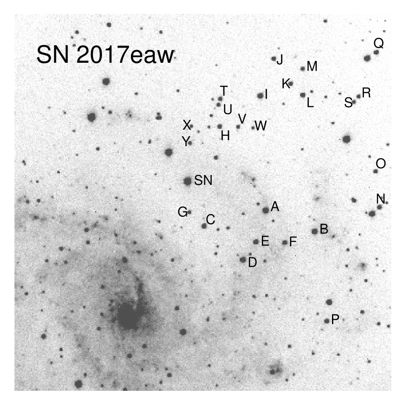
Figure 1: KAIT $R$-band image from 2017 June 23 showing a $6{\farcm}7\times 6{\farcm}7$ field, including SN 2017eaw and the local sequence of calibration stars (labeled) listed in Table 1. North is up and east is to the left.

Table 1: Photometric Sequence around SN 2017eaw

Star	$B$ (mag)	$V$ (mag)	$R$ (mag)	$I$ (mag)
A	14.788	14.138	13.756	13.332
B	15.176	14.404	13.956	13.482
C	16.006	15.140	14.640	14.135
D	16.032	14.836	14.154	13.507
E	16.288	15.346	14.805	14.332
F	15.878	15.379	15.079	14.686
G	17.444	16.490	15.942	15.367
H	16.830	15.923	15.400	14.843
I	15.534	14.670	14.172	13.689
J	17.073	15.935	15.285	14.637
K	16.923	16.015	15.492	14.955
L	16.345	15.401	14.859	14.315
M	17.081	16.191	15.677	15.152
N	17.632	16.078	15.195	14.330
O	17.044	16.080	15.526	14.982
P	16.824	15.637	14.960	14.330
Q	16.358	15.530	15.051	14.548
R	17.520	16.436	15.816	15.229
S	17.394	16.400	15.831	15.274
T	16.870	15.884	15.317	14.779
U	17.387	16.494	15.980	15.475
V	18.008	16.764	16.055	15.365
W	18.489	17.387	16.757	16.116
X	18.274	16.994	16.266	15.583
Y	17.291	16.384	15.861	15.324

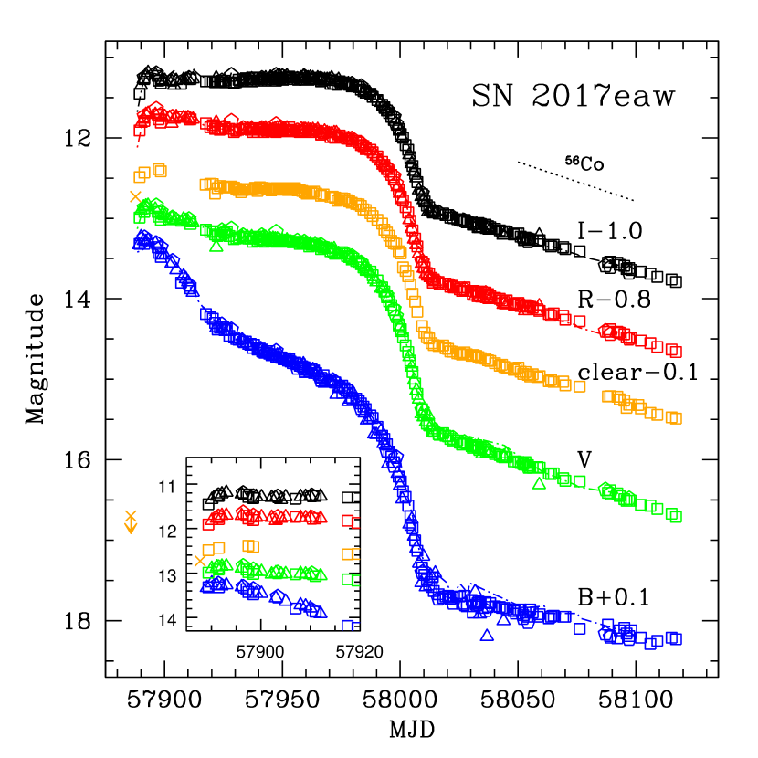
Figure 2: The BVRI and unfiltered (clear; orange points) light curves of SN 2017eaw. KAIT data are shown as open squares, Nickel data as open pentagons, and pt5m data as open triangles. We also include our remeasurements of the discovery and upper limit to discovery from Wiggins (2017) as orange crosses (see Section 6.1). For comparison we include the BVRI light curves from Tsvetkov et al. (2018; dotted-dashed curves). We also show the expected decline rate if the exponential tail of the light curve is powered by the decay of ⁵⁶Co. In the inset we focus on the first 35 days of the light curves; the offsets for the curves are of the same magnitude as in the main figure.

We combined all of the photometry from the three telescopes, covering from about 1 day after the discovery by Wiggins (2017) through nearly the end of calendar year 2017. We show the light curves for SN 2017eaw in Figure 2. The curves seem to exhibit a conspicuous initial “bump” near maximum brightness (see the figure inset), followed by an extended plateau phase, a steady rapid decline from the plateau, and an exponential tail (see, e.g., Anderson et al. 2014). In the figure we also compare with the previously published BVRI light curves from Tsvetkov et al. (2018) at (approximately) matching epochs. The agreement is quite good, with $\Delta B=0.04\pm 0.09$, $\Delta V=0.00\pm 0.05$, $\Delta R=0.00\pm 0.04$, and $\Delta I=0.06\pm 0.04$ mag, in the sense of “ours$-$Tsvetkov et al.” A similar comparison with the photometry of Rui et al. (2019) results in $\Delta B=0.04\pm 0.05$, $\Delta V=0.04\pm 0.04$, $\Delta R=0.03\pm 0.02$, and $\Delta I=0.05\pm 0.02$ mag, again in the sense of “ours$-$Rui et al.,” indicating that their photometry was slightly brighter, particularly in the redder bands. Rui et al. also began monitoring the SN about 1 day before we did.

We have not performed $S$-corrections (Stritzinger et al. 2002) to our photometry. Nevertheless, we have made a comparison of all of the photometry obtained between the three telescopes and instruments: $\Delta B=-0.06\pm 0.09$, $\Delta V=-0.02\pm 0.05$, $\Delta R=-0.01\pm 0.05$, and $\Delta I=-0.01\pm 0.04$ mag, “KAIT$-$pt5m”; $\Delta B=0.01\pm 0.12$, $\Delta V=-0.03\pm 0.04$, $\Delta R=-0.03\pm 0.05$, and $\Delta I=-0.02\pm 0.03$ mag, “Nickel$-$pt5m”; and, $\Delta B=-0.04\pm 0.06$, $\Delta V=0.02\pm 0.03$, $\Delta R=0.00\pm 0.03$, and $\Delta I=0.00\pm 0.03$ mag, “KAIT$-$Nickel.” As one can see, the differences are quite small. We also have generated synthetic photometry from the Lick Observatory Kast spectra that we obtained (see Section 2.2) using pysynphot (STScI Development Team 2013) with the KAIT, Nickel, and pt5m bandpasses, comparing with the photometry at or near contemporaneous epochs (these spectra were all first recalibrated to the $V$ magnitude for the nearest epoch), and find the following: $\Delta(B-V)=-0.31\pm 0.14$, $\Delta(V-R)=0.00\pm 0.05$, $\Delta(V-I)=0.11\pm 0.04$ mag, “KAIT$-$phot”; $\Delta(B-V)=-0.27\pm 0.12$, $\Delta(V-R)=0.05\pm 0.05$, $\Delta(V-I)=-0.10\pm 0.06$ mag, “Nickel$-$phot”; and, $\Delta(B-V)=0.06\pm 0.10$, $\Delta(V-R)=0.05\pm 0.05$, $\Delta(V-I)=0.13\pm 0.05$ mag, “pt5m$-$phot.” One could therefore correct our photometry by these amounts, although we caution that the blue end of the KAIT and Nickel $B$ bandpasses extends shortward of the bluest wavelengths of the spectra, so there is likely flux missing within those bandpasses; likewise, the spectra extend redward of the end of the Nickel $I$ bandpass trace, so, again, not all of the flux may be represented in the synthetic photometry with that filter. The authors will happily provide the bandpasses to the reader should an inquiry be made.

We analyze the photometric properties of SN 2017eaw more extensively in Section 6.

Table 2: Log of Optical Spectroscopy of SN 2017eaw

Obs. Date	MJD	Age	Instrument	Wavelength	Resolution
				Range (Å)	(Å)
17-05-17.402	57890.902	5.2	MMT-BC	5697–6997	0.49
17-05-19.481	57892.981	7.3	Kast	3650–10650	2.0
17-05-20.377	57893.877	8.2	Kast	3660–10600	2.0
17-05-20.429	57893.929	8.2	MMT-BC	5785–7090	0.49
17-05-21.482	57894.982	9.3	MMT-BC	5788–7093	0.49
17-06-02.231	57906.731	21.0	HIRES	3642.9–7967.1	0.02–0.03
17-06-02.478	57906.978	21.3	Kast	3660–10630	2.0
17-06-21.480	57925.980	40.3	Kast	3622–10718	2.0
17-06-24.418	57928.918	43.2	MMT-BC	5711–7022	0.49
17-06-27.500	57932.000	46.3	Kast	3627–10718	2.0
17-06-30.351	57934.851	49.2	MMT-BC	5709–7020	0.49
17-07-01.468	57935.968	50.3	Kast	3638–10710	2.0
17-07-17.488	57951.968	66.3	Kast	3614–10690	2.0
17-07-26.498	57960.998	75.3	Kast	3622–10680	2.0
17-07-30.489	57964.989	79.3	Kast	3620–10708	2.0
17-08-01.488	57966.988	81.3	Kast	3620–10710	2.0
17-08-27.492	57992.992	107.3	Kast	3620–10716	2.0
17-08-29.166	57994.666	109.0	Bok-B&C	3684–8040	3.6
17-09-12.330	58008.830	123.1	Bok-B&C	4000–8039	3.6
17-09-14.191	58010.691	125.0	Kast	3632–10720	2.0
17-09-27.155	58023.655	138.0	Kast	3630–10680	2.0
17-09-29.249	58025.749	140.0	Bok-B&C	3799–8029	3.6
17-10-08.149	58034.649	148.9	MMT-BC	3476–8695	1.9
17-10-09.100	58035.600	149.9	MMT-BC	5705–7010	0.49
17-10-11.117	58037.617	151.9	Bok-B&C	4731–9079	3.6
17-10-19.346	58045.846	160.1	Kast	3622–10670	2.0
17-10-25.330	58051.830	166.1	Kast	3620–10680	2.0
17-10-27.080	58053.580	167.9	MMT-BC	5646–6958	0.49
17-10-28.113	58054.613	168.9	Bok-B&C	4415–8728	3.6
17-10-30.100	58056.600	170.9	Kast	3622–10706	2.0
17-11-20.091	58077.591	191.9	MMT-BC	5657–6965	0.49
17-11-26.099	58083.599	197.9	Kast	3630–10700	2.0
17-12-12.098	58099.598	213.9	Kast	3632–10680	2.0
17-12-18.096	58105.596	219.9	Kast	3632–10712	2.0
18-01-13.093	58131.593	245.9	Kast	3630–10680	2.0
18-07-01.415	58300.915	415.2	MMT-BC	5720–7025	0.49
18-09-06.316	58367.816	482.1	MMT-BC	3245–8104	1.9

2.2 SN Optical Spectroscopy

Over an eight-month period beginning on 2017 May 19, a series of 20 optical spectra of SN 2017eaw were obtained with the Kast double spectrograph (Miller & Stone 1993) mounted on the 3 m Shane telescope at Lick Observatory. These spectra were taken at or near the parallactic angle (Filippenko 1982) to minimize slit losses caused by atmospheric dispersion. Data were reduced following standard techniques for CCD processing and spectrum extraction (Silverman et al. 2012) utilizing IRAF routines and custom Python and IDL codes. Low-order polynomial fits to arc-lamp spectra were used to calibrate the wavelength scale, and small adjustments derived from night-sky lines in the target frames were applied. Observations of appropriate spectrophotometric standard stars were used to flux-calibrate the spectra.

With the Blue Channel (BC) spectrograph on the MMT we also obtained nine spectra with the 1200 lines mm^-1 grating, with a central wavelength of 6360 Å and a 1$\farcs$0 slit width, and two spectra with the 300 lines mm^-1 grating. We obtained five epochs of optical spectroscopy with the Boller $\&$ Chivens (B$\&$C) spectrograph mounted on the 2.3 m Bok telescope on Kitt Peak using the 300 line mm^-1 grating.

Standard reductions were carried out using IRAF, and wavelength solutions were determined using internal He-Ne-Ar lamps. Flux calibration was achieved using spectrophotometric standards at a similar airmass taken throughout the night.

Additionally, some of us (H.I., I.J.M.C., D.H., M.R.K.) obtained an optical spectrum of SN 2017eaw with the HIRES spectrometer (Vogt et al. 1994) on the Keck I 10 m telescope on Maunakea on 2017 June 2. The spectrum, with an exposure time of 292 s, has a continuum signal-to-noise ratio (S/N) of 40 per pixel at 5500 Å. The use of the $0{\farcs}87\times 14{\farcs}0$ (C2) decker provided a resolution of 50,000; while sky subtraction can be performed, the extra on-sky pixels in the spatial direction provide additional information about the environment of the primary target. The spectrum was reduced using the standard California Planet Search pipeline (Howard et al. 2010).

We provide a log of the Kast, MMT, Bok, and Keck observations in Table 2. The sequence of Kast and MMT spectra is shown in Figure 3. All of the spectra have been corrected for the redshift of NGC 6946, taken to be $z=0.000133$. We can see from the sequence in Figure 3 that SN 2017eaw appears to be a normal SN II-P.

Figure 3: Sequence of Kast, MMT, and Bok spectra of SN 2017eaw; see Table 2. The spectra have all been corrected for the redshift of the host galaxy, but not for the reddening to the SN. The spectra are labeled by the day since explosion, assumed to be JD 2,457,885.7 (see Section 6.1).

2.3 Pre-SN HST Imaging

The site of SN 2017eaw was observed serendipitously by several HST programs prior to explosion. These include GO-14156 (PI A. Leroy) with the Wide Field Camera 3 (WFC3) IR channel in bands F110W (total exposure 455.87 s) and F128N (1411.74 s) on 2016 February 9, and GO-14638 (PI K. Long) with WFC3/IR F160W (396.93 s) on 2016 October 24; and GO-9788 (PI L. Ho) with the Advanced Camera for Surveys (ACS) Wide Field Channel (WFC) on 2004 July 29 in F658N (700 s) and F814W (120 s), and GO-14786 (PI B. Williams) with ACS/WFC on 2016 October 26 in F814W (2570 s) and F606W (2430 s).

2.4 Pre-SN Spitzer Imaging

The SN site was also serendipitously observed pre-explosion by a number of programs on various dates, from 2004 June 10 to 2017 March 31, using Spitzer. We list all of these observations and the data that we considered in Table 3. The data were obtained primarily with the Infrared Array Camera (IRAC; Fazio et al. 2004), but also with the Multiband Imaging Photometer for Spitzer (MIPS; Rieke et al. 2004). The IRAC imaging was obtained both during the cryogenic mission in all four bands (3.6, 4.5, 5.8, and 8.0 $\mu$m), and during the so-called “Warm” (post-cryogenic) mission only in the two shortest wavelength bands. For MIPS we consider only the available 24 $\mu$m data.

Table 3: Log of Spitzer Data Covering the SN 2017eaw Site

Obs. Date	AORKEY	Data
04-06-10	5508864	IRAC 3.6, 4.5, 5.8, 8.0 $\mu$m
04-07-10	5576704	MIPS 24, 70, 160 $\mu$m
04-07-11	5576960	MIPS 24, 70, 160 $\mu$m
04-09-12	10550528	IRAC 3.6, 4.5, 5.8, 8.0 $\mu$m
04-11-25	5508608	IRAC 3.6, 4.5, 5.8, 8.0 $\mu$m
04-11-25	10550784	IRAC 3.6, 4.5, 5.8, 8.0 $\mu$m
05-07-19	14526976	IRAC 3.6, 4.5, 5.8, 8.0 $\mu$m
05-07-20	14456320	IRAC 3.6, 4.5, 5.8, 8.0 $\mu$m
05-07-20	14457856	IRAC 3.6, 4.5, 5.8, 8.0 $\mu$m
05-09-24	14528000	MIPS 24 $\mu$m
05-12-30	14528256	IRAC 3.6, 4.5, 5.8, 8.0 $\mu$m
06-01-10	14528512	MIPS 24 $\mu$m
06-11-26	17965568	IRAC 3.6, 4.5, 5.8, 8.0 $\mu$m
06-12-29	18277120	IRAC 3.6, 4.5, 5.8, 8.0 $\mu$m
07-01-06	18270976	MIPS 24 $\mu$m
07-07-03	18277376	IRAC 3.6, 4.5, 5.8, 8.0 $\mu$m
07-07-10	18271232	MIPS 24 $\mu$m
07-12-27	23508224	IRAC 3.6, 4.5, 5.8, 8.0 $\mu$m
08-01-27	24813824	IRAC 3.6, 4.5, 5.8, 8.0 $\mu$m
08-07-18	27190016	IRAC 3.6, 4.5, 5.8, 8.0 $\mu$m
08-07-29	27189248	MIPS 24 $\mu$m
09-08-06	34777856	IRAC 3.6, 4.5 $\mu$m
10-01-05	34778880	IRAC 3.6, 4.5 $\mu$m
10-08-13	39560192	IRAC 3.6, 4.5 $\mu$m
11-07-27	42195456	IRAC 3.6, 4.5 $\mu$m
11-08-01	42415872	IRAC 3.6, 4.5 $\mu$m
12-02-01	42502144	IRAC 3.6, 4.5 $\mu$m
13-08-17	48000768	IRAC 3.6, 4.5 $\mu$m
14-01-03	49665024	IRAC 3.6, 4.5 $\mu$m
14-02-17	48934144	IRAC 3.6, 4.5 $\mu$m
14-03-26	50623232	IRAC 3.6, 4.5 $\mu$m
14-09-16	50623744	IRAC 3.6, 4.5 $\mu$m
14-10-15	50623488	IRAC 3.6, 4.5 $\mu$m
15-01-31	53022464	IRAC 3.6, 4.5 $\mu$m
15-09-02	52785664	IRAC 3.6, 4.5 $\mu$m
15-09-07	52785920	IRAC 3.6, 4.5 $\mu$m
15-09-16	52786176	IRAC 3.6, 4.5 $\mu$m
15-09-28	52786432	IRAC 3.6, 4.5 $\mu$m
15-10-27	52786688	IRAC 3.6, 4.5 $\mu$m
15-11-25	52786944	IRAC 3.6, 4.5 $\mu$m
15-12-23	52787200	IRAC 3.6, 4.5 $\mu$m
16-09-04	52787456	IRAC 3.6, 4.5 $\mu$m
16-10-12	60832256	IRAC 3.6, 4.5 $\mu$m
16-12-30	60832512	IRAC 3.6, 4.5 $\mu$m
17-03-31	60832768	IRAC 3.6, 4.5 $\mu$m

2.5 Post-explosion HST Imaging

We observed SN 2017eaw on 2017 May 29.79 with HST WFC3/UVIS in subarray mode in F814W (270 s total exposure), as part of our Target of Opportunity (ToO) program (GO-14645, PI S. Van Dyk). Although the SN was quite bright at the time, we successfully avoided saturating the detector (the F814W band was expressly chosen to reduce the probability of this happening on the likely observing date), while achieving appreciable S/N on fainter point-like objects in the SN environment that could be used as astrometric fiducials (see Section 7.1). SN 2017eaw was also observed on 2018 January 5 with WFC3/UVIS in F555W and F814W (710 and 780 s) as part of the HST Snapshot program GO-15166 (PI A. Filippenko); unfortunately, the SN was still quite bright ($V\approx 16.8$ and $I\approx 14.8$ mag) at the time, and the central pixels of the SN image are saturated, further leading to prominent detector row and column bleeding.

3 Extinction to SN 2017eaw

What is noticeable in the spectral sequence is the presence of a strong Na i D feature, consistent with the large Galactic extinction we would expect for a host galaxy at a Galactic latitude of only $b=11{\fdg}7$. Of course, at low resolution the Na i feature could also include a contribution to the extinction internal to the host, given its low redshift. As mentioned in Section 2.2, we obtained a Keck HIRES spectrum, with the aim of isolating both the Na i D and 5780 Å diffuse interstellar band (DIB) features, to assess the amount of extinction to the SN. We show the HIRES spectrum in Figure 4 for these two portions of the overall coverage. As one can see, the Na i D1 and D2 lines are essentially saturated; however, these are both at wavelengths corresponding essentially to zero redshift (i.e., to the Galactic component of extinction), whereas at wavelengths corresponding to NGC 6946, no clear sign of either feature exists. Phillips et al. (2013) cautioned that Na i D is a rather poor measure of the value of the extinction and recommended use of the DIB $\lambda$5780 feature instead. One can see in Figure 4 that a strong DIB feature is evident; however, again this corresponds to the foreground extinction component, whereas any contribution from the host cannot be distinguished from the broad Galactic feature. Hence, we conclude that there is little evidence for significant host-galaxy extinction. Hereinafter we therefore assume the Galactic foreground contribution toward SN 2017eaw from Schlafly & Finkbeiner (2011) (via NED), $A_{V}=0.941$ mag, as the total visual interstellar extinction. The uncertainty in the extinction is likely $\lesssim 0.1$ mag.

Figure 4: Portions of the spectrum of SN 2017eaw obtained with HIRES on the Keck I telescope on 2017 June 2, focusing on the Na i D lines (left panel) and the DIB $\lambda$5780 feature (right panel). The locations of these features at the host-galaxy redshift are indicated (by “host”) in both panels.

4 Distance to SN 2017eaw

Not surprisingly for such a famous and well-studied galaxy as NGC 6946, NED lists 32 redshift-independent distances. These include Tully-Fisher estimates of 5.0–5.3 Mpc by Bottinelli et al. (1984; 1986), 5.4–5.5 Mpc by Schoniger & Sofue (1994), and 5.5 Mpc by Pierce (1994). A number of SN-based distances have also been estimated, including early measurements with the expanding photosphere method (EPM) applied to SN 1980K by Schmidt et al. (1992) (7.2 Mpc) and Schmidt et al. (1994) (5.7 Mpc), with more recent attempts using SN 2004et by Takáts & Vinkó (2012) (4.8 Mpc) and Bose & Kumar (2014) (4.0–5.9 Mpc). The standardized candle method (SCM) has also been applied to SN 2004et by Olivares E. et al. (2010) (4.3–5.4 Mpc) and Pejcha & Prieto (2015) (4.5 Mpc), and applied with a modified version of this method by Poznanski et al. (2009) to SN 2002hh (6.0 Mpc) and SN 2004et (4.7 Mpc). Thus, most of these distance estimates to NGC 6946 have been quite “short,” at approximately 5 Mpc. Karachentsev et al. (2000) estimated 6.8 Mpc using the brightest blue stars in a galaxy group containing NGC 6946, and Tikhonov (2014) measured a tip-of-the-red-giant-branch (TRGB) distance to NGC 6946 of $6.72\pm 0.15$ Mpc using archival HST data.

We have independently estimated a TRGB distance using more recent HST data. We downloaded publicly available deep archival WFC3/UVIS images in F606W (total exposure 5470 s) and F814W (5548 s) for a parallel field $6{\farcm}9$ from the galaxy center, obtained on 2016 October 28 by GO-14786 (PI B. Williams). We were well underway analyzing this field when the work by Murphy et al. (2018) appeared. These authors analyzed a different field, also observed by GO-14786 in the same bands to approximately the same depth, but at a nuclear offset of $7{\farcm}9$. Murphy et al. inferred an astonishingly larger distance of $7.83\pm 0.29$ Mpc (i.e., a distance modulus of $29.47\pm 0.08$ mag), much greater than previous estimates. To confirm this measurement and to potentially bolster confidence in the measurement from our chosen field, we decided to undertake analysis of both fields, shown in Figure 5. We note that yet another TRGB analysis, by Anand et al. (2018), appeared, also while our analysis was underway.

Both fields have comparatively fewer contaminants, e.g., younger supergiants, in NGC 6946 than other archival HST pointings in these bands and likely better probe the desired older halo population. We processed the data with Dolphot (Dolphin 2000; 2016), with the same input parameters as described in Section 7.1 after first running the individual frames corrected for charge-transfer-efficiency (CTE) through AstroDrizzle, to flag cosmic-ray hits. We further culled out objects from the output photometry list that are most probably “good stars,” by imposing cuts on the Dolphot parameters object type ($=1$), and sharpness $s$ ($-0.3\leq s\leq 0.3$), crowding ($<0.5$ mag), quality flag ($=0$), and $\chi$ ($<2$ at F606W and $<3$ at F814W), following, e.g., Mager et al. (2008). Even with these cuts we cannot rule out that source crowding and confusion are affecting the photometry. The photometry for these selected objects was then corrected for the appropriate Galactic foreground extinction in each band (Schlafly & Finkbeiner 2011) toward each of the two fields. Field B is less extinguished than is Field A. The extinction varies up to 0.01 mag in both $A_{V}$ and $A_{I}$ for Field A, and to 0.03 and 0.02 mag in $A_{V}$ and $A_{I}$, respectively, for Field B.

We transformed the reddening-corrected photometry at F814W to the color-dependence-corrected brightness $QT$, following Jang & Lee (2017) for the HST appropriate camera and filter combination. The resulting color-magnitude diagrams (CMDs) for the two fields are shown in Figures 6 and 7 for A and B, respectively. A prominent red giant branch can be clearly seen in both of the figures. We applied two different Sobel edge detectors, the [$-1$, $-1$, $-1$, 0, 0, 0, $+1$, $+1$, $+1$] kernel from Madore et al. (2009) and the [$-1$, $-2$, $-1$, 0, $+1$, $+2$, $+1$] kernel from Jang & Lee (2017), to 0.05-mag-binned histograms of $QT$ in the color range $1.1\leq(F606W-F814W)_{0}\leq 2.0$ mag, to mitigate against contamination from the likely RSGs near $(F606W-F814W)_{0}\approx 1.0$ mag and to locate the TRGB. We show the resulting edge detector responses in Figures 6 and 7 as well. By trial and error we had found that these two edge detectors provided the clearest discrimination of the TRGB; as can be seen in the figures, their results are quite similar.

From our analysis the TRGB appears to be at 25.40 and 25.42 mag for Fields A and B, respectively. The RGB is more populated in Field A than in Field B. For the uncertainties in these two estimates we assumed the width of a Gaussian fit to the edge detector response (Sakai et al. 1999; 2000) for the two fields, which are 0.23 and 0.20 mag, respectively. Taking the uncertainty-weighted mean of these two estimates, and assuming the luminosity of the TRGB is $QT=-4.031$ mag (Jang & Lee 2017; this is the value for the similar late-type spiral galaxy NGC 4258), we found a reddening-corrected distance modulus to NGC 6946 of $29.44\pm 0.21$ mag, or a distance of $7.73\pm 0.78$ Mpc.

Note that we arrive at the same value, to within the uncertainties, for both the TRGB apparent brightness and the distances as did Murphy et al. (2018) and Anand et al. (2018; $7.72\pm 0.32$ Mpc, from analysis of both Fields A and B), via somewhat less sophisticated pathways to the TRGB estimate (we used the Sobel edge detection, whereas the other two studies used a Bayesian maximum likelihood technique; see their studies for details).

To demonstrate that the TRGB distance estimate for NGC 6946 is reasonable, we compare in Figure 8 the CMD for the combined fields A and B with a CMD of a field in NGC 4258, considered a distance anchor by Jang & Lee (2017). The TRGB distance for the latter galaxy ($7.18\pm 0.40$ Mpc; Mager et al. 2008) is consistent with distance estimates obtained using that galaxy’s nuclear water megamaser ($7.54\pm 0.17$ Mpc; e.g., Riess et al. 2016). It is evident from the figure that the TRGB distance to NGC 6946 is comparable to that of NGC 4258, with the former galaxy being slightly more distant than the latter. The TRGB distance to NGC 6946 is inconsistent with the previous shorter SN-based distances. We note that general comparisons of Cepheid and TRGB distance estimates have been in excellent agreement (e.g., Jang et al. 2018).

Hereinafter we adopt our estimate, above, of the distance to NGC 6946. As a cross-check, we also computed SCM and EPM distances to SN 2017eaw in Section 6.6.

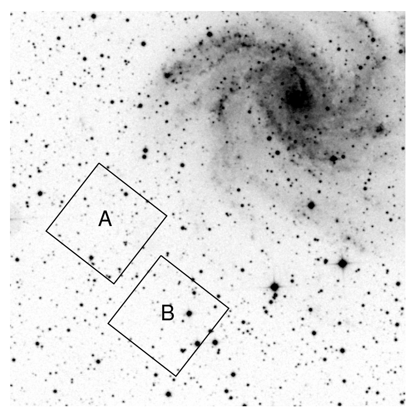
Figure 5: Digitized Sky Survey image of the host galaxy, NGC 6946, showing the footprints of the two WFC3/UVIS fields, A and B, that we analyzed when determining the TRGB distance to the galaxy. Field A is at a galactic nuclear offset of $6{\farcm}9$, while Field B is at $7{\farcm}9$. The latter field had been previously analyzed by Murphy et al. (2018). Both fields were also analyzed by Anand et al. (2018).

Figure 6: Left: CMD of the color-dependence-corrected brightness $QT$ (Jang & Lee 2017) versus the reddening-corrected $(F606W-F814W)$ color for stars in Field A (see Figure 5), which is $6{\farcm}9$ from the center of NGC 6946. Representative uncertainties in the photometry are also shown. A well-developed red giant branch can clearly be seen. Middle: histogram of $QT$, binned by 0.05 mag, for stars in the color range $(F606W-F814W)_{0}=1.1$–2.0 mag. Right: the Sobel edge detector responses, from Madore et al. (2009; solid red curve) and Jang & Lee (2017; dotted-dashed blue curve), that we applied to the histogram in the middle panel. A dashed line indicates the TRGB at $QT=25.40$ mag, which is at the peak of a Gaussian fit to the edge detector responses. The width of that Gaussian is 0.23 mag.

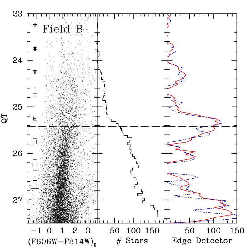
Figure 7: Left: CMD of the color-dependence-corrected brightness $QT$ (Jang & Lee 2017) versus the reddening-corrected $(F606W-F814W)$ color for stars in Field B (see Figure 5), which is $7{\farcm}9$ from the center of NGC 6946. Representative uncertainties in the photometry are also shown. A well-developed red giant branch can clearly be seen. Middle: histogram of $QT$, binned by 0.05 mag, for stars in the color range $(F606W-F814W)_{0}=1.1$–2.0 mag. Right: the Sobel edge detector responses, from Madore et al. (2009; solid red curve) and Jang & Lee (2017; dotted-dashed blue curve), that we applied to to the histogram in the middle panel. A dashed line indicates the TRGB at $QT=25.42$ mag, which is at the peak of a Gaussian fit to the edge detector responses. The width of that Gaussian is 0.20 mag. Note that Murphy et al. (2018) had previously performed this analysis for this field and found essentially the same value for the TRGB brightness. Anand et al. (2018) also found a similar value.

Figure 8: Left: CMD of the color-dependence-corrected brightness $QT$ (Jang & Lee 2017) vs. the reddening-corrected $(F606W-F814W)$ color for stars in the combined Fields A and B in NGC 6946 (see Figure 5). Right: a similar CMD for stars in the halo of the late-type spiral galaxy NGC 4258 (see Jang & Lee 2017). The long-dashed line in both panels indicates the detected level of the TRGB in each galaxy. The short-dashed line in the left panel indicates where the TRGB would be if the distance to NGC 6946 were 5.2 Mpc.

5 Metallicity of the SN 2017eaw Site

One means of estimating the metallicity at the site of a SN is from an abundance gradient for the host galaxy, if it has been established. Since the oxygen abundance is often adopted as a proxy for metallicity, the gradient considered is usually that of oxygen. First, we deprojected an image of NGC 6946 assuming the relevant galaxy parameters (inclination, position angle) from Jarrett et al. (2003). From the absolute positions of SN 2017eaw and the NGC 6946 nucleus, the nuclear offset of the SN site is then $\sim 221\arcsec$. At the assumed host distance, this corresponds to 7.3 kpc. Using the oxygen abundance gradient from Belley & Roy (1992; although they assumed a distance of 5.9 Mpc to NGC 6946), we estimate that the abundance at the SN 2017eaw site is $12+\log({\rm O/H})=8.71\pm 0.05$. With the Sun’s oxygen abundance assumed to be $12+\log({\rm O/H})=8.69\pm 0.05$($Z=0.014$; Asplund et al. 2009), this would imply a solar-like metallicity at the SN site.

Another, potentially more accurate, way of estimating the SN site metallicity is from the O abundances of nearby emission regions, if available (e.g., Modjaz et al. 2011). Examination of the archival HST F658N image reveals that no such regions exist in the SN’s immediate environment. Fortunately, Gusev et al. (2013) measured the O abundance for three H ii regions nearest the SN site, #2, #22, and #23 (all $\sim 73\arcsec$ to the northwest), to be $12+\log({\rm O/H})=8.46\pm 0.01$, $8.56\pm 0.02$, and $8.46\pm 0.01$, respectively; the next closest, #6, $\sim 92\arcsec$ to the southeast, has $12+\log({\rm O/H})=8.58\pm 0.02$. All of these measurements would imply that the SN 2017eaw site is somewhat subsolar in metallicity. Given that this method is likely a more direct means of estimating the metallicity, we adopt hereinafter a subsolar metallicity in the range of $Z=0.009$ ([Fe/H] = $-$0.2) to $Z=0.011$ ([Fe/H] = $-$0.1).

6 Analysis of SN 2017eaw

6.1 Date of Explosion

Not many observational constraints exist on the explosion epoch of SN 2017eaw. For instance, the KAIT SN search did not obtain its first image of the host (independent of the multiband SN 2017eaw monitoring) until 2017 June 12.99, nearly a month after discovery, owing to hour-angle limitations imposed for the search. Steele & Newsam (2017) did not detect the SN on 2017 May 6.18 to $R>21.2$ mag, eight days prior to discovery. Wiggins (2017) reported that nothing was detected at the SN position to an unfiltered mag ${>19}$ on May 12.20, $\sim 2$ days before his discovery. Interestingly, Drake et al. (2017) reported detection of a source at the SN position in the Catalina Real-Time Transient Survey (CRTS) data at $V\approx 19.8$ mag on 2017 May 7.43, slightly more than one day later than the deep upper limit by Steele & Newsam.

Patrick Wiggins kindly provided his unfiltered images both of the discovery and of the pre-discovery upper limit. We analyzed the images with DAOPHOT, using our photometric sequence at $R$ from Table 1 for calibration. We confirmed that the SN was discovered at 12.8 mag. However, we found that the nondetection limit on 2017 May 12 was $>16.8$ mag, rather than $>19$ mag.

Additionally, Andrew Drake graciously provided us with four nearly contemporaneous CRTS exposures from 2017 May 7, which were the basis of their report (Drake et al. 2017). We analyzed these images both individually and as a coaddition. In short, we could not convince ourselves that the SN had been detected on that date. In more detail, we compared the coadded CRTS image astrometrically, first with a good-quality KAIT image of the SN, and subsequently with the archival HST images in which the SN progenitor is detected (see Section 7.1), using 25 and 13 stars in common between the two image datasets, respectively. In the coadded image there is indeed what appears to be a source within 1 pixel of the nominal SN position. However, DAOPHOT did not detect this source, and therefore we were not able to measure its brightness. Additionally, just a hint of this source appears only in one of the four individual exposures.

Nevertheless, with the Wiggins discovery and pre-discovery nondetection, in particular, we can employ knowledge of the rise time of SNe II-P to place a further constraint on the explosion date. Specifically, we draw upon the beautifully defined rise of KSN 2011a (Garnavich et al. 2016), which appears to be a relatively normal SN II-P, albeit at higher redshift than SN 2017eaw. In Figure 9 we show a comparison of the very early KSN 2011a light curve with the $R$-band and unfiltered SN 2017eaw light curves. We note, of course, that the Kepler bandpass used to detect KSN 2011a is far broader than $R$, although comparable in breadth to the unfiltered KAIT CCD response function (Riess et al. 1999). Assuming that the rise of the latter was similar to that of the former (and the comparison tends to imply that this is the case), we can infer that the explosion date for SN 2017eaw was on about JD 2,457,885.7 (May 12.2). The Wiggins nondetection constrains this date to about $\pm 0.1$ day, which is remarkable. The implied rapid rise time of SN 2017eaw would also rule out the CRTS “pre-discovery,” some five days prior to the Wiggins discovery. Our assumed explosion date is almost exactly a day earlier than the date assumed by Rui et al. (2019).

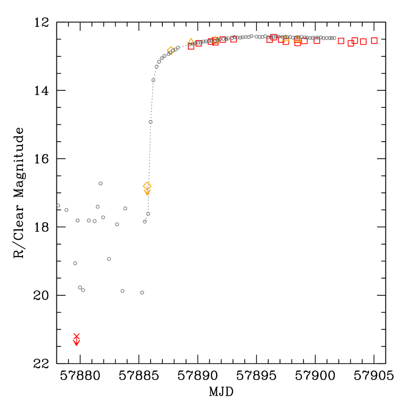
Figure 9: The rise of SN 2017eaw compared to that of KSN 2011a (Garnavich et al. 2016). Shown are the $R$-band (red open squares) and KAIT unfiltered (orange open triangles) light curves for SN 2017eaw. The discovery and pre-discovery nondetection by Wiggins (2017) are shown as orange open diamonds; the $R$ nondetection by Steele & Newsam (2017) is shown as a red cross. The very early KSN 2011a light curve is represented by open gray circles.

6.2 Absolute Light and Color Curves

We corrected the observed BVRI light curves of SN 2017eaw for the assumed Galactic foreground extinction and then adjusted them to be absolute light curves with our adopted distance modulus to NGC 6946. As an illustration we show the absolute $V$ curve in Figure 10. At maximum $V=-17.57$ mag, SN 2017eaw is generally more luminous than SN 1999em (Hamuy et al. 2001; Leonard et al. 2002a; Elmhamdi et al. 2003b), SN 1999gi (Leonard et al. 2002b), and SN 2012aw (Bose et al. 2013; Dall’Ora et al. 2014). However, it is intermediate in luminosity between these SNe and SN 2004et (Sahu et al. 2006; Maguire et al. 2010; when adjusted to our assumed distance to NGC 6946), which appears to be significantly more luminous than SN 2017eaw. (See also the comparison of SN 2017eaw with SN 2004et by Tsvetkov et al. 2018.) The bump in the light curve near maximum brightness (at $\sim 8$ days after explosion) appears more prominent for SN 2017eaw, and not nearly as pronounced for the other SNe, although Morozova et al. (2018) required $\lesssim 0.3\ M_{\odot}$ of dense circumstellar matter (CSM) to account for enhanced emission in the early-time curves of SN 1999em, SN 2004et, and SN 2012aw. (SN 2004et may have exhibited a less prominent, more extended bump peaking at about 20 days post-explosion.) We have also fit via a minimum $\chi^{2}$ the simple model from Elmhamdi et al. (2003b), shown in the figure, for the behavior of the light curve. See Section 6.4 for the ramifications of this fit.

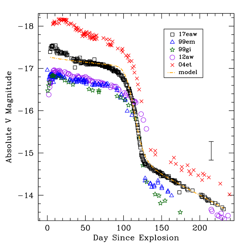
Figure 10: Absolute $V$ light curve of SN 2017eaw (black open squares). For comparison we show the absolute curves of SN 1999em (Hamuy et al. 2001; Leonard et al. 2002a; Elmhamdi et al. 2003b; blue open triangles), SN 1999gi (Leonard et al. 2002b; dark green open stars), SN 2004et (Sahu et al. 2006; Maguire et al. 2010; red crosses), and SN 2012aw (Bose et al. 2013; Dall’Ora et al. 2014; purple open circles), all adjusted by the distances and reddenings in the literature, although SN 2004et was adjusted to our assumed distance to NGC 6946. The displayed error bar is representative of the average uncertainty in the SN 2017eaw curve, with the predominant source of error being the uncertainty in the adopted distance modulus to NGC 6946. Also shown is a simple model for the behavior of the light curve, following Elmhamdi et al. (2003b; yellow dotted-dashed curve).

The color evolution of SN 2017eaw is shown in Figure 11. Generally, reasonably close agreement exists between this SN and other SNe II-P, such as SN 1999em, SN 1999gi, SN 2004et, and SN 2012aw. SN 1999gi may have been somewhat redder than SN 2017eaw in all colors, while SN 2004et appears to have been bluer in all of our observed colors, especially at early and later times.

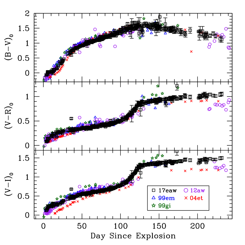
Figure 11: $B-V$, $V-R$, and $V-I$ color curves (black open squares) for SN 2017eaw, corrected for our assumed value of the reddening to the SN. For comparison we show the color curves for the SNe II-P 1999em (Hamuy et al. 2001; Leonard et al. 2002a; Elmhamdi et al. 2003b; blue open triangles), 1999gi (Leonard et al. 2002b; dark green open stars), 2004et (Sahu et al. 2006; red crosses), and 2012aw (Bose et al. 2013; Dall’Ora et al. 2014; purple open circles), all corrected by the reddening assumed by those studies and adjusted in time to match approximately the curves for SN 2017eaw.

6.3 Bolometric Light Curve

With an absence of photometry both shortward and longward of BVRI, we transformed the absolute observed light curves to a bolometric light curve via several different methods. One method was to assume bolometric corrections to the broadband photometry derived from the modeling of SNe II-P by Pejcha & Prieto (2015). Similarly, we also used the bolometric corrections from Bersten & Hamuy (2009). Another was to assume bolometric corrections derived empirically and more generally for SNe II by Lyman et al. (2014), and more specifically for SN 2004et and SN 1999em relative to the $R$ band by Maguire et al. (2010). Finally, we produced a bolometric light curve from extrapolations of blackbody fits to the observed BVRI datapoints, using the routine superbol (Nicholl 2018). The fitting with this routine was initially set relative to the observed $V$-band maximum, which was on JD 2,457,893.06. We note that we just missed the actual $V$ maximum: fitting a Gaussian function approximately to the early bump in the observed light curve, we estimate that the time of $V$ maximum likely occurred around JD 2,457,893.7.

The ensemble of results from these various methods indicates a general trend for the bolometric light curve, and so we computed an average from all of these various results. However, the earliest portion of the curve ($\lesssim 25$ days) was established only from the average of the bolometric corrections from Bersten & Hamuy (2009) and Pejcha & Prieto (2015) and the superbol fit, since the former two corrections tend to agree with the early blackbody fitting when the SN was still hot ($T>8000$ K) and relatively free from emission lines. We consider it less likely that the early behavior of the curves resulting from the corrections from Maguire et al. (2010) and Lyman et al. (2014) adequately represents the actual early-time bolometric evolution of SN 2017eaw. In a forthcoming paper (V. Morozova et al. 2019, in preparation), we will demonstrate that the bolometric light curve — particularly the early peak — is consistent with the presence of dense CSM immediately adjacent to the progenitor at the time of explosion. Such CSM is strongly suspected to be present for a number of SNe II-P (Moriya et al. 2017; 2018; Morozova et al. 2017; 2018; Förster et al. 2018; Paxton et al. 2018) and could be related to pre-explosion outbursts during the late stages of RSG nuclear burning (e.g., Quataert & Shiode 2012; Shiode & Quataert 2014; Fuller 2017). The behavior of the curve on the exponential tail is likely more consistent with that resulting from the bolometric correction from Lyman et al. (2014) and the bolometric correction for SN 1999em from Maguire et al. (2010) than the superbol blackbody extrapolation, which is affected by the presence of strong spectral emission lines during this phase and overpredicts the luminosity on the tail. The uncertainty in our average curve conservatively includes the individual uncertainties in the superbol fit and in the individual bolometric corrections.

For comparison we also show the bolometric light curves for SN 2004et (Maguire et al. 2010; Faran et al. 2018; after adjusting their published curves from their respective assumed distances to the distance of NGC 6946 that we assume) and SN 1987A (Suntzeff & Bouchet 1990). The former SN, again, appears to have been more luminous than SN 2017eaw, except possibly at peak.

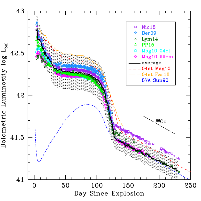
Figure 12: Bolometric light curve of SN 2017eaw, which we adopt as the average (solid curve) of various methods: The blackbody-fitting routine superbol (Nicholl 2018; Nic18, purple open squares) and bolometric corrections from Bersten & Hamuy (2009; Ber09, light blue stars), Lyman et al. (2014; Lym14, darkgreen crosses), Pejcha & Prieto (2015; PP15, green open triangles), and Maguire et al. (2010; Mag10, cyan open circles for SN 2004et and magenta open pentagons for SN 1999em, both relative to $R$-band). The hashed region indicates the conservative 1$\sigma$ uncertainty in our adopted curve. Also shown for comparison are bolometric light curves for SN 2004et from Maguire et al. (2010; red short-dashed curve, adjusted to our assumed distance from their adopted distance of $5.9\pm 0.4$ Mpc) and Faran et al. (2018; Far18, orange long-dashed curve, adjusted from their adopted distance of $4.81\pm 0.16$ Mpc), and of SN 1987A (Suntzeff & Bouchet 1990; Sun90, dark-blue short-dashed-dotted curve). Also indicated is the expected decline rate for the light-curve tail if it is powered primarily by the decay of ⁵⁶Co (long-dashed-dotted curve).

6.4 Estimate of the Nickel Mass

We can estimate the mass, $M({{}^{56}{\rm Ni}})$, of radioactive nickel, whose daughter is ⁵⁶Co, the decay of which powers the exponential tail of SN II-P light curves via deposition and trapping of $\gamma$-rays released by the decay. For a given SN II-P, assuming that the $\gamma$-ray thermalization is equally efficient, the comparison is usually made to SN 1987A, the bolometric light curve of which (Suntzeff & Bouchet 1990) we show in Figure 12. The luminosities of the light-curve tails for the two SNe after about day 135 are comparable, if not the same, to within the uncertainties. The nickel mass for SN 1987A was estimated at $M_{\rm Ni}=0.075\pm 0.015\ M_{\odot}$ (Arnett & Fu 1989), so it is likely safe to assume that $M_{\rm Ni}$ for SN 2017eaw is essentially the same, based on this comparison. Another means of estimating $M_{\rm Ni}$ is via a “steepness” parameter, $S$, introduced by Elmhamdi et al. (2003a) for the $V$-band light curve. We show a best fit of their simple analytical model for the behavior of the $V$ curve in Figure 10. From that model fit we find that $S=0.089$ mag day^-1 at an “inflection point” of day 113.6. From Elmhamdi et al. (2003a; their Equation (3)) we then estimate that $M_{\rm Ni}=0.04\ M_{\odot}$, which is about a factor of two less than the SN 1987A comparison. Rho et al. (2018) found that dust had started forming as early as day 124, so there may be an increase in extinction local to the SN that could decrease the luminosity of the exponential tail. However, we note that Rho et al. arrived at satisfactory model fits of their near-infrared nebular spectra assuming that $M_{\rm Ni}=0.084\ M_{\odot}$, which is consistent with the SN 1987A-based value. The uncertainty in $M_{\rm Ni}$ for SN 2017eaw, based on our bolometric light curve, is $\sim\pm 0.03\ M_{\odot}$. An estimate of $\sim 0.07$–$0.08\ M_{\odot}$ is consistent with the trend that Valenti et al. (2016) (their Figure 22) found for SNe II, given $M_{V}=-17.13$ at day 50 for SN 2017eaw.

6.5 Spectral Analysis

We compared our spectra of SN 2017eaw with the template spectra in both SNID (Blondin & Tonry 2007) and GELATO (Harutyunyan et al. 2008). With SNID the SN 2017eaw spectra compared best with other SNe II-P, such as SN 2006bp, SN 1999em, SN 2005dz, SN 2004fx, SN 2004et, and (at later times) even with SN 1987A. For the GELATO comparison the best matches were with SN 1999gi and, most often, SN 2004et.

At very early times ($\leq 10$ days) some SNe II-P have shown “flash” features in their spectra indicative of an explosion within dense CSM. The features arise from recombination of the CSM ionized by the UV/X-ray flash from shock breakout (Khazov et al. 2016). (We mention that Kochanek 2019, however, has explained the flash spectral features via a collision interface formed between the regular stellar winds in a binary system.) In Figure 13 we show our SN 2017eaw spectra within the first nine days or so after explosion. We have also included here the earliest available spectrum of SN 2017eaw of which we are aware, obtained by Xiang et al. (2017) and shown by Rui et al. (2019). Xiaofeng Wang graciously permitted us to present this spectrum in the figure. We compare these spectra with some examples that have exhibited prominent flash features, the SNe II PTF12krf and PTF11iqb (Khazov et al. 2016; also Smith et al. 2015), as well as the SN IIb iPTF13ast (SN 2013cu; Gal-Yam et al. 2014; Khazov et al. 2016), which is among the first known instances of this phenomenon. The spectra of PTF12krf, PTF11iqb, and iPTF13ast are from days 4${}^{+1}_{-1}$, 2.1${}^{+0}_{-1.1}$, and 3${}^{+0}_{-0.2}$, respectively. Various emission features — H$\alpha$, H$\beta$, He ii $\lambda$4686, and an N iii $\lambda\lambda$4634, 4640/C iii $\lambda\lambda$4647, 4650, 4651 blend — are all strong in the early spectra of the latter three SNe. However, for SN 2017eaw there may be only quite weak indications of these features in the spectrum by Xiang et al. and in our earliest MMT spectrum from day 5.2, in particular at H$\alpha$. Rui et al. (2019) argued that in the day 2.6 spectrum the weak H$\alpha$ feature is indicative of slow-moving (163 km s^-1) CSM, although we see no evidence of this in our day 5.2 spectrum, and instead only weak H$\alpha$ near zero rest-frame velocity. By the day 7.3 spectrum any traces of these features have vanished.

It is possible therefore that either spectra were not obtained sufficiently early and the features were missed, or these flash features were just intrinsically weaker for SN 2017eaw than for the notable cases that do show them. If the latter is the case, then, as noted earlier, an implication is that any CSM in immediate proximity to SN 2017eaw may have been too dense and massive for these features to form. Alternatively, narrow lines might have been hidden if the CSM was asymmetric, as in the case of PTF11iqb, which had early SN IIn-like signatures present and an enhanced early luminosity peak that declined to a plateau (Smith et al. 2015). In order to explain the rapid disappearance of the narrow lines, while the excess CSM interaction luminosity remained, Smith et al. (2015) proposed that a highly asymmetric CSM geometry, such as a disk, could allow the opaque SN ejecta to envelop the CSM interaction occurring in a disk. In that scenario, CSM interaction would continue to generate luminosity, which would heat the SN ejecta and produce a larger emergent luminosity, but it would be buried inside the opaque ejecta, so that the narrow lines are hidden from view. This type of asymmetric CSM interaction might also help to explain the lack of narrow lines during the initial peak of SN 2017eaw.

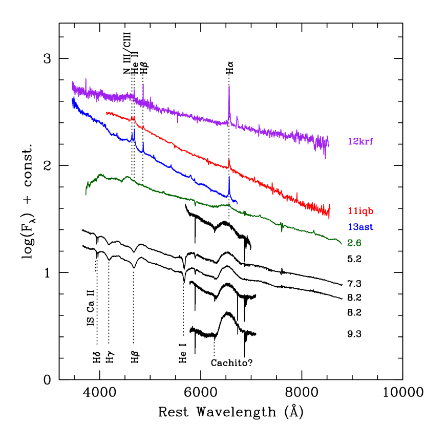
Figure 13: Spectra of SN 2017eaw in the first $\sim 9$ days after explosion. For comparison we show the spectra of three SNe II that showed flash-ionization features, indicative of the presence of CSM — PTF12krf (Khazov et al. 2016), PTF11iqb (Smith et al. 2015; Khazov et al. 2016), and iPTF13ast (SN 2013cu; Gal-Yam et al. 2014; Khazov et al. 2016). The ages, in days, of the SN 2017eaw spectra are labeled. The spectra of PTF12krf, PTF11iqb, and iPTF13ast are from days 4${}^{+1}_{-1}$, 2.1${}^{+0}_{-1.1}$, and 3${}^{+0}_{-0.2}$, respectively. Various emission and absorption features are indicated.

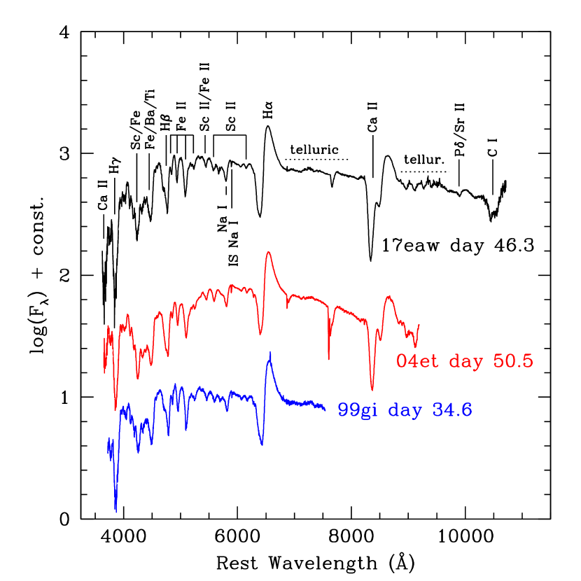
Figure 14: Comparison of the day 46.3 spectrum of SN 2017eaw with spectra of two SNe II-P, SN 2004et (Sahu et al. 2006), and SN 1999gi (Leonard et al. 2002b), at comparable ages during the plateau phase. Various spectral lines and features are indicated. Telluric lines have not been removed from the spectrum of SN 2004et, and may be weakly present in the spectrum of SN 2017eaw.

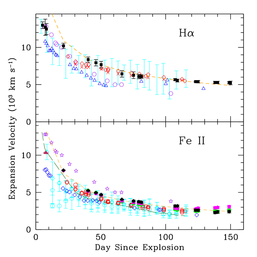
Figure 15: Evolution of the expansion velocity of SN 2017eaw. Top panel: From H$\alpha$ absorption, solid black points; data for SN 1999em (Leonard et al. 2002a, open blue triangles), SN 2012aw (Bose et al. 2013, open purple circles), SN 2004et (Sahu et al. 2006, red crosses; Maguire et al. 2010, open red diamonds), and the range of the sample of 96 SNe II-P from Gutiérrez et al. (2017) (cyan error bars) shown for comparison. Bottom panel: from Fe ii line absorption, solid green circles ($\lambda$4924), solid magenta pentagons ($\lambda$5018), and solid black diamonds ($\lambda$5169); data for SN 1999em (Leonard et al. 2002a, $\lambda$5169, open blue diamonds), SN 1999gi (Leonard et al. 2002b, photospheric velocity, dark green long-dashed line), SN 2012aw (Bose et al. 2013, all spectral lines, open purple stars), SN 2004et (Sahu et al. 2006, $\lambda$4924, red open circles, $\lambda$5018, red open pentagons, $\lambda$5169, red open diamonds; Maguire et al. 2010, average, red open squares), and the sample of Gutiérrez et al. (2017) ($\lambda$4924, cyan open circles, $\lambda$5018, cyan open pentagons, $\lambda$5169, cyan open diamonds). The measurements for SN 2017eaw from He i $\lambda$5876 absorption are shown as maroon solid triangles. Also shown in both panels are the trends for SNe II-P found by Faran et al. (2014) (orange short-dashed line).

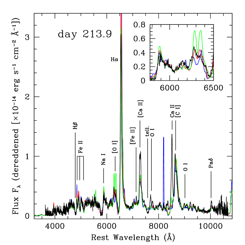
Figure 16: Lick/Kast low-resolution spectrum of SN 2017eaw obtained on day 213.9 (black curve); see Section 2.2. The spectrum has been dereddened following our assumed value for the reddening to the SN (Section 3). We compare the SN 2017eaw spectrum with model spectra on day 212 from Jerkstrand et al. (2012), assuming a progenitor at $M_{\rm ZAMS}=12\ M_{\odot}$ (blue curve), $15\ M_{\odot}$ (red curve), and $19\ M_{\odot}$ (green curve). The model spectra have been scaled in flux to the observed spectrum. Various spectral lines and features are indicated. The inset in the figure focuses on the spectral region containing the Na i D $\lambda\lambda$5890, 5896 and [O i] $\lambda\lambda$6300, 6364 lines.

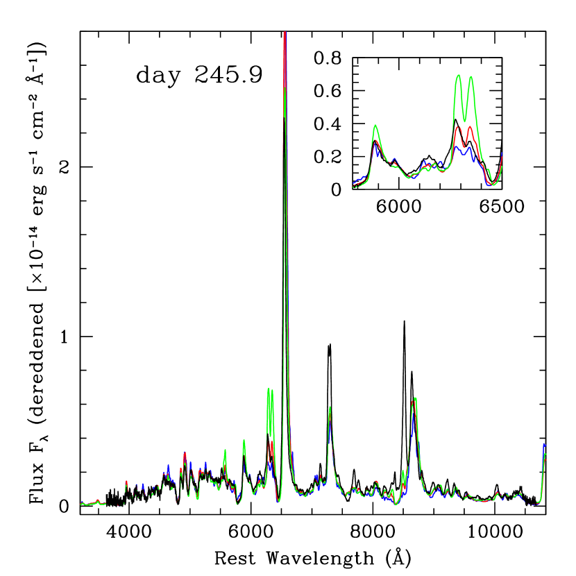
Figure 17: Lick/Kast low-resolution spectrum of SN 2017eaw obtained on day 245.9 (black curve); see Section 2.2. The spectrum has been dereddened following our assumed value for the reddening to the SN (Section 3). We compare the SN 2017eaw spectrum with model spectra on day 249 from Jerkstrand et al. (2012), assuming a progenitor at $M_{\rm ZAMS}=12\ M_{\odot}$ (blue curve), $15\ M_{\odot}$ (red curve), and $19\ M_{\odot}$ (green curve). The model spectra have been scaled in flux to the observed spectrum. Similar spectral features are seen as in Figure 16. The inset in the figure focuses on the spectral region containing the Na i D $\lambda\lambda$5890, 5896 and [O i] $\lambda\lambda$6300, 6364 lines.

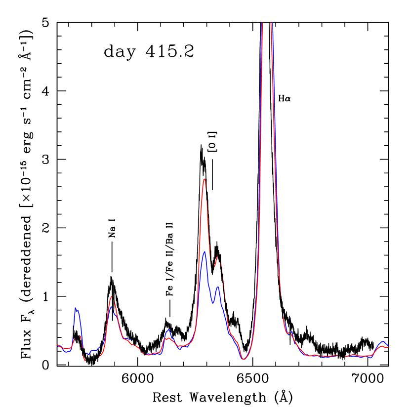
Figure 18: MMT moderate-resolution spectrum of SN 2017eaw obtained on day 415.2 (black curve); see Section 2.2. The spectrum has been dereddened following our assumed value for the reddening to the SN (Section 3). This spectrum only covers the region containing the Na i D $\lambda\lambda$5890, 5896 and [O i] $\lambda\lambda$6300, 6364 lines (plus H$\alpha$). We compare the SN 2017eaw spectrum with model spectra generated by Jerkstrand et al. (2012) at progenitor mass $M_{\rm ZAMS}=12\ M_{\odot}$ (blue curve) and $15\ M_{\odot}$ (red curve) on day 400. (No model is available at $M_{\rm ZAMS}=19\ M_{\odot}$ for this epoch.) The model spectra have been scaled in flux to the observed spectrum. Various spectral lines and features are indicated.

The primary absorption features in the early-time spectra are the Balmer lines, He i $\lambda$5876, the strong Na i D line (discussed above), and what is likely interstellar Ca ii, also due to the Galactic foreground. The Balmer profiles continue to develop their characteristic P-Cygni-like appearance over time, and He i is no longer visible by or before day 39. It is possible that in our moderate-resolution data we see (weakly) the “Cachito” feature discussed by Gutiérrez et al. (2017) to the blue side of H$\alpha$. However, the feature as observed in SN 2017eaw is comprised not of one wide absorption, but of two narrow (FWHM $\approx 100$ km s^-1) absorption minima that evolve very little over time, with respect to both profile substructure and wavelength position. The position overlaps with a grouping of O₂ absorption lines centered near 6280 Å, so some telluric contamination is possible. If the feature is associated with H$\alpha$, then its velocity in the earliest spectrum is $-$13,300 km s^-1. The feature is not discernible in our spectra beyond day 47.9. We note that this feature does bear striking resemblance to persistent absorptions blueshifted with respect to H$\alpha$ that are sometimes observed in SNe IIb (Milisavljevic et al. 2013). The origin of these high-velocity features is unclear, and explanations involving ejecta asymmetry, a mixture with Fe ii or Si ii lines, and interaction with CSM have been put forward (Baron et al. 1994; Zhang & Wang 1996; James & Baron 2010; Milisavljevic et al. 2013).

At later times during the plateau phase, the spectra evolved gradually. We show an example spectrum in Figure 14 from day 46.3. When we compare this spectrum using SNID we obtain a best match with SN 2004et (Sahu et al. 2006). Using GELATO the best comparison is with SN 1999gi (Leonard et al. 2002b). We show the spectra for these two other SNe II-P in the figure for comparison. The comparison shows that, spectroscopically, SN 2017eaw is evidently quite normal. We have indicated various features in these spectra (including a few telluric lines primarily in the spectrum of SN 2004et), following Gutiérrez et al. (2017): the Balmer profiles, Na i, Ca ii, and various metal lines of Fe ii, Sc ii, and blends. We may also see evidence for the C i $\lambda$10,691 line.

We measured the evolution of the expansion velocity of SN 2017eaw from our multi-epoch spectra, starting with our earliest spectrum on day 5.2 through well off the plateau on day 151.9. Velocities were estimated from the minimum of the absorption features of the H$\alpha$, He i $\lambda$5876, and Fe ii $\lambda\lambda$4924, 5018, 5169 lines. Multiple measurements were performed to estimate uncertainties. See Figure 15. We compared the evolution of the expansion velocity of SN 2017eaw to the sample of 96 SNe II from Gutiérrez et al. (2017), as well as to other well-studied SNe II, including SN 1999em (Leonard et al. 2002a), SN 1999gi (Leonard et al. 2002b), SN 2004et (Sahu et al. 2006; Maguire et al. 2010), and SN 2012aw (Bose et al. 2013). We also show the trends in velocity evolution from Faran et al. (2014). The expansion velocities of SN 2017eaw are generally within the mean of all SNe II-P, although the expansion velocities from Fe ii $\lambda$5169 are somewhat higher, particularly at the earliest epochs.

We can also analyze the spectra at ages that are among the latest available (213.9, 245.9, and 415.2 days) in light of the modeling of the nebular spectra of SN 2004et by Jerkstrand et al. (2012) at comparable ages. (These models were also applied to the nebular spectra of SN 2012aw; Jerkstrand et al. 2014.) We show these three observed spectra once again in Figures 16, 17, and 18, after dereddening them (see Section 3; assuming the reddening law of Cardelli et al. 1989 with $R_{V}=3.1$), along with the model spectra for initial masses $M_{\rm ZAMS}=12$, 15, and $19\ M_{\odot}$ at days 212, 250, and 400, respectively (a $19\ M_{\odot}$ model on day 400 is not available). For each figure we have photometrically scaled the model spectra to the observed one, via pysynphot, using the light-curve data closest in time to the observed spectrum on day 213.9; for the day 245.9 and day 415.2 spectra, we had to linearly extrapolate the light curves at $V$ and $R$, respectively. We especially focus in the figure on the spectral region containing the Na i D $\lambda\lambda$5890, 5896 and [O i] $\lambda\lambda$6300, 6364 lines, whose strengths (as Jerkstrand et al. 2012 pointed out) are most influenced by the assumed progenitor initial mass. One can see that the observed spectra at all three epochs are best matched by the $15\ M_{\odot}$ model, with the $12\ M_{\odot}$ model generally underpredicting and the $19\ M_{\odot}$ model overpredicting the line strengths (on days 213.9 and 245.9), particularly for [O i]. In total, the implication of this comparison is that the progenitor initial mass of SN 2017eaw is closest to $15\ M_{\odot}$.

6.6 SN-based Distance Estimates

Table 4: Quantities Derived from the EPM Analysis of SN 2017eaw

Age	$\theta_{BV}$	$T_{BV}$	$\zeta_{BV}$	$\theta_{BVI}$	$T_{BVI}$	$\zeta_{BVI}$	$\theta_{VI}$	$T_{VI}$	$\zeta_{VI}$
(days)	($10^{8}$ km Mpc-1)	(K)		($10^{8}$ km Mpc-1)	(K)		($10^{8}$ km Mpc-1)	(K)
21.3	20.67(0.40)	7473(189)	0.716(0.021)	21.47(0.40)	8041(96)	0.595(0.005)	21.52(0.36)	8578(133)	0.543(0.003)
40.3	26.27(3.33)	5032(627)	1.256(0.243)	25.55(2.71)	6056(339)	0.774(0.051)	24.84(0.88)	7227(352)	0.594(0.021)
46.3	26.54(0.84)	4818(123)	1.350(0.058)	26.22(0.92)	5730(80)	0.828(0.015)	26.04(0.56)	6739(163)	0.629(0.014)
50.3	26.94(0.52)	4684(73)	1.416(0.038)	26.51(0.55)	5582(47)	0.857(0.010)	26.40(0.27)	6573(76)	0.643(0.007)

Primarily to provide a check on our TRGB distance estimate to the host galaxy (see Section 4), we also estimated distances to SN 2017eaw itself through the SCM (Hamuy & Pinto 2002; Nugent et al. 2006) and the EPM (Kirshner & Kwan 1974; Eastman & Kirshner 1989; Schmidt et al. 1992). To compute the SCM distance, we closely followed the technique of Polshaw et al. (2015) and input the values directly drawn from our data into their Equation 1: the $I$ brightness on day 50, $I_{50}=12.29\pm 0.01$ mag; the extinction at $I$ to SN 2017eaw, $A_{I}=0.517$ mag (with a very conservative uncertainty of 0.1 mag); and, the expansion velocity on day 50, $v_{50}=4697\pm 103$ km s^-1, which we estimated from the Fe ii $\lambda$5169 absorption line in our spectrum on day 50.3 ($\sim$ day 50; see Figure 15). For all other constants and their uncertainties, we adopted the values provided by Polshaw et al. Our resulting distance estimate from SCM is then $7.32\pm 0.60$ Mpc.

For the EPM distance estimate, we only considered spectral epochs earlier than 60 days (i.e., 21.3, 40.8, 46.7, and 50.2 days) after explosion that included the Fe ii $\lambda$5169 absorption feature. We adopted the velocities measured from that spectral feature as representing the photospheric velocity, $v_{\rm phot}$. We considered the photometry data of the SN that were as contemporaneous as possible with the spectral epochs. We assumed our estimate of the extinction to the SN (Section 3). We also adopted the dilution factors from Dessart & Hillier (2005). (We note that dilution factors have also been generated more recently by Vogl et al. 2019 and are in good agreement with those of Dessart & Hillier.) To implement the EPM to estimate the theoretical angular size, $\theta$, of the photosphere, we closely followed the procedure detailed by Leonard et al. (2002b). We carried out this procedure for each of three bandpass combinations ($BV$, $BVI$, and $VI$) to determine the photospheric temperatures ($T$) and appropriate dilution factors ($\zeta$); see Table 4.

To estimate the distances using each of the bandpass combinations, we fixed the explosion date ($t_{0}$) to be our adopted value, JD 2,457,885.7 (see Section 6.1). We feel confident that we can do this, given how well the rise time of the SN appears to be constrained. We then merely measured the slope of the best-fitting line (via weighted least-squares) describing the relation between the day since explosion and the ratio $\theta/v_{\rm phot}$ for each of the three combinations; see Figure 19. Uncertainties in each of the three slopes were established by determining the 1$\sigma$ dispersion in model slopes generated from 1000 simulated datasets characterized by the parameter values and uncertainties in Table 4, together with the uncertainty in the assumed reddening and a flat likelihood of $\pm 1$ day uncertainty around $t_{0}$ (which contributed $\sim 0.25$ Mpc to the total uncertainty). We then calculated the unweighted mean of the three slopes (which were all quite similar in value, $\sim 7.3$ Mpc, as can be seen in the figure) as our final EPM distance estimate. Since the three distance values are not independent, we conservatively report the final uncertainty as the sum in quadrature of the largest uncertainty in an individual distance and the 1$\sigma$ dispersion in the three individual distances. Our distance estimate from EPM is then $7.27\pm 0.42$ Mpc.

We note that both of the uncertainties given for the SCM and EPM estimates are purely statistical in nature and do not reflect potential systematics inherent in both techniques. Nevertheless, these estimates appear to corroborate the TRGB distance we have estimated for NGC 6946 (see Section 4).

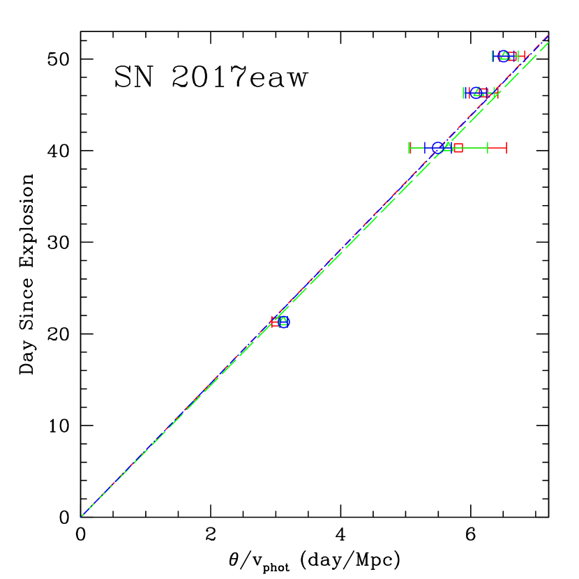
Figure 19: EPM fitting for SN 2017eaw for three combinations of bandpasses, $BV$ (red open squares, short-dashed line), $BVI$ (green open triangles, long-dashed line), and $VI$ (blue open circles, short-dashed-dotted line). We have fixed the explosion time, $t_{0}$, to our adopted date of JD 2,457,885.7 (Section 6.1). See text for further details.

7 The SN Progenitor

7.1 Identification of the Progenitor

Table 5: Photometry of the SN 2017eaw Progenitor

Instrument	Band	Obs. Date	Magnitude
HST ACS/WFC	F606W	16-10-26	26.40(05)
HST ACS/WFC	F658N	04-07-29	$>$24.6
HST ACS/WFC	F814W	04-07-29	22.60(04)
HST ACS/WFC	F814W	16-10-26	22.87(01)
HST WFC3/IR	F110W	16-02-09	20.32(01)
HST WFC3/IR	F128N	16-02-09	19.69(02)
HST WFC3/IR	F160W	16-10-24	19.36(01)
Spitzer IRAC	3.6 $\mu$m	15-12-23 – 17-03-31	18.01(03)
Spitzer IRAC	4.5 $\mu$m	15-12-23 – 17-03-31	17.80(04)
Spitzer IRAC	5.8 $\mu$m	04-06-10 – 08-07-18	$>$16.15
Spitzer IRAC	8.0 $\mu$m	04-06-10 – 08-01-27	$>$15.47
Spitzer MIPS	24 $\mu$m	04-07-09 – 04-07-11	$>$10.39

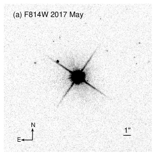
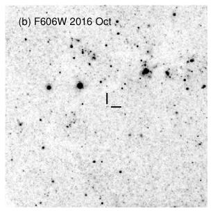
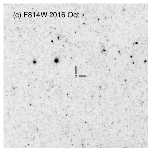
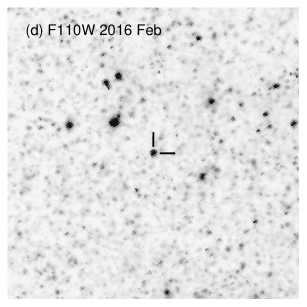
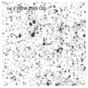
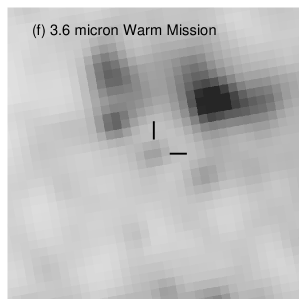
Figure 20: (a) Portion of the HST WFC3/UVIS image mosaic of SN 2017eaw in F814W the SN 2017eaw obtained on 2017 May 29; the SN is the brightest object in the image. (b) Portion of the pre-explosion ACS/WFC image mosaic in F606W from 2016 October 26, with the likely candidate for the SN progenitor indicated with tick marks. (c) Same as for (b), but at F814W. (d) Same as for (b), but for WFC3/IR F110W from 2016 February 9. (e) Same as for (b), but for WFC3/IR F160W from 2016 October 24. (f) Same as for (b), but in the Spitzer IRAC 3.6 $\mu$m band during the “Warm” (post-cryogenic) Mission (data from 2009 August 6 through 2017 March 31). All panels are shown to the same scale and orientation. North is up and east is to the left.

We (Van Dyk et al. 2017) were the first initially to identify a stellar object in the optical/near-infrared with characteristics indicative of an RSG and not far from the nominal position of the SN in a ground-based image, when matched to the pre-SN HST data. However, we noted then that high-spatial-resolution imaging of the SN was required to confirm this candidate. We astrometrically registered our 2017 WFC3 ToO image mosaic at F814W to the 2004 ACS/WFC F814W exposure (the 2004 image was publicly available in 2017 May, whereas the 2016 F814W data were not). Using 25 stars in common between the two datasets, we registered the images to an rms uncertainty of 0.37 ACS/WFC pixel (18.5 mas). The difference between the transformed centroid of the SN and the centroid of the candidate object is 0.31 pixel, within the 1$\sigma$ astrometric uncertainty. We therefore consider it highly likely that this object is the progenitor of SN 2017eaw. We show the ACS and WFC3 images at the same scale and orientation in Figure 20. The progenitor candidate is indicated in the figure. We note that Johnson et al. (2018), Kilpatrick & Foley (2018), and Rui et al. (2019) also identified this object as the SN progenitor in their studies.

The pre-SN HST images obtained from the HST archive had been pre-processed with the standard pipeline at STScI. We measured photometry from all of the pre-SN HST images with Dolphot. First, we processed the individual CTE-corrected frames through AstroDrizzle to flag cosmic-ray hits. We then set the Dolphot parameters FitSky=3, RAper=8, and InterpPSFlib=1 and used the default TinyTim model PSFs. We list the resulting (Vegamag) photometry in Table 5. The progenitor candidate was detected in all bands, except F658N, for which we provide a 3$\sigma$ upper limit estimate of the star’s brightness. Our measurements in these bands roughly agree with those presented by Kilpatrick & Foley (2018) and Rui et al. (2019), although both of these studies included a measurement in the F164N band from HST program GO-14786, whereas we considered that this would contribute little additional insight into the progenitor SED, since the bandpass of the F164N filter is encompassed by that of F160W, and therefore did not include it. As both Kilpatrick & Foley (2018) and Rui et al. (2019) noted, the brightness of the progenitor appears to have dimmed somewhat at F814W between 2004 and 2016.

Our progenitor detections in the HST data are consistent with the conservative upper limit ($R>22.4$ mag) that Steele & Newsam (2017) placed on detection.

7.2 Analysis of the Spitzer Data

As Khan (2017) pointed out, the progenitor candidate is clearly detected at 3.6 and 4.5 $\mu$m; see Figure 20. We know that RSGs, particularly of high luminosity, experience variability in the optical (e.g., Soraisam et al. 2018), although Johnson et al. (2018) appeared to have ruled out significant variability at the $\gtrsim 5$–10% level for the SN 2017eaw progenitor within the decade prior to explosion. Tinyanont et al. (2019) have also ruled out any variability at $K_{s}$ greater than 6% lasting longer than 200 days from 1 yr to 1 day before explosion. Given the large amount of available Spitzer data, we were able to explore possible variability of the progenitor at 3.6 and 4.5 $\mu$m, during both the cryogenic and “Warm” (post-cryogenic) missions. We note that Kilpatrick & Foley (2018) performed a similar analysis. For each of the observation dates listed in Table 3 we analyzed the Spitzer individual artifact-corrected basic calibrated data (cBCDs) with MOPEX and APEX (Makovoz & Khan 2005; Makovoz & Marleau 2005; Makovoz et al. 2006). We performed point-response-function (PRF) fitting photometry with the APEX User List Multiframe module, forcing the model PRF to find and fit the progenitor at its absolute position. In addition to the progenitor, we also forced the PRF fitting on two objects of similar brightness, both southwest of the progenitor, one at $3{\farcs}5$ (it can be seen in Figure 20(f)) and the other at $13{\farcs}2$.

To successfully avoid oversubtracting the PRF from the progenitor and the two comparison objects against the complex galactic background, within the Extract Med Filter module of APEX we adjusted (decreased) the values of Window X, Window Y, and Outliers per Window from the default values and visually inspected the residual image created with the task APEX_QA. The photometry was executed in exactly the same way for all three objects. For each epoch we created with MOPEX an array-location-dependent photometric correction mosaic for each of the two bands, the correction factors from which we applied to the photometry. (This correction is very close to unity, in general.) The photometry was further aperture- and pixel-phase-corrected; the progenitor photometry was further color-corrected assuming a 3500 K blackbody appropriate for an RSG (this correction was also very close to unity).

We show the multi-epoch photometry at 3.6 and 4.5 $\mu$m for all three objects in Figure 21. One can readily see that the scatter in the datapoints for all three objects far exceeds the formal APEX uncertainties, and the scatter may, in fact, be somewhat correlated for all three, indicating that the photometry of objects at this brightness level in the Spitzer data may be dependent both on the image quality and on the photometric extraction technique. Although the objects were formally detected at an appreciable S/N in the majority of epochs in both bands, the objects, including the progenitor, are still quite faint relative to the background and are in close proximity to brighter objects; assessing the degree of oversubtraction or undersubtraction of the PRF model was therefore quite subjective, and the formal photometric uncertainties almost certainly underrepresent the actual uncertainties.

From this analysis we can rule out any detectable variability in the progenitor at these wavelengths at the $\sim 0.5$–0.6 mag level over the nearly 13 yr prior to explosion. One could potentially better investigate the existence of any variability below this level in the two Spitzer bands through the template-subtraction technique. One would have to wait, though, ostensibly until the SN has faded sufficiently at 3.6 and 4.5 $\mu$m to provide for an adequate template. As of the end of 2018, SN 2017eaw is still quite bright as seen by Spitzer (Tinyanont et al. 2019), and given the limited lifetime of the Spitzer mission, it may not be possible to acquire the desired images in time. We may need to turn to the James Webb Space Telescope (JWST) to obtain the templates, degrading the resolution to match the existing Spitzer data before subtraction.

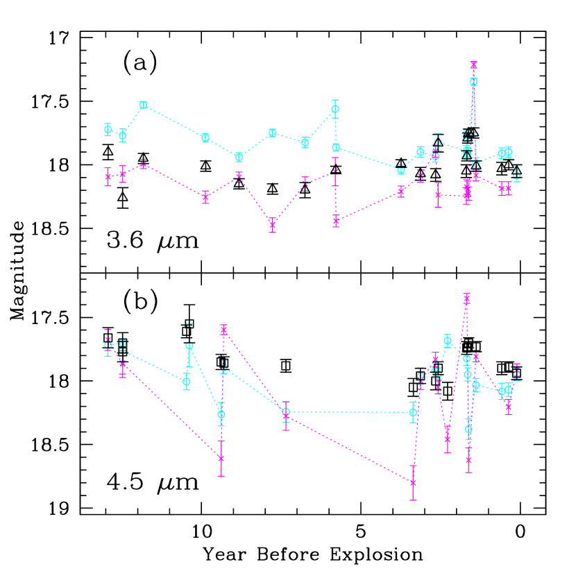
Figure 21: Apparent brightness of the SN 2017eaw progenitor in the Spitzer (a) 3.6 $\mu$m (open triangles) and (b) 4.5 $\mu$m (open squares) bands over $\sim 12.9$ yr prior to explosion. We also show measurements for two objects in the Spitzer data with comparable brightness in the vicinity of the progenitor, one at $3{\farcs}5$ (open cyan circles) and the other $13{\farcs}2$ (magenta crosses), both to the southwest of the progenitor.

7.3 Modeling of the Progenitor SED

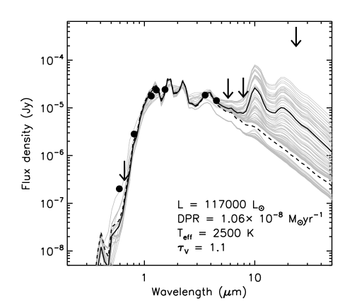
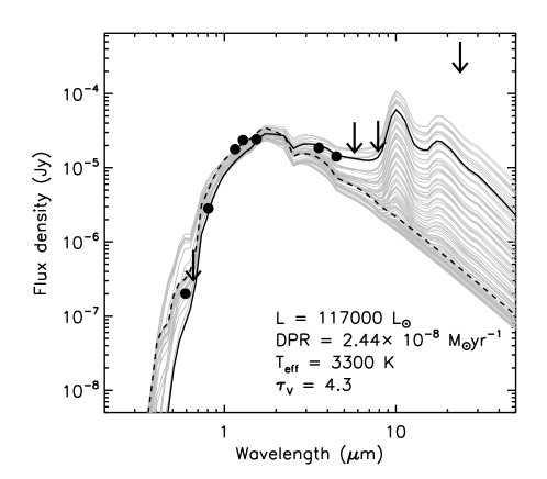
Figure 22: Reddening-corrected observed SED for the SN 2017eaw progenitor (solid points and upper limits). The measurements are from pre-explosion HST and Spitzer images (see Table 5). The solid curves are the GRAMS models (Sargent et al. 2011; Srinivasan et al. 2011), with the black curve being the best-fit model, and the gray curves being the family of 100 models with acceptable fit quality, when $T_{\rm eff}$ is allowed to be a free parameter (top panel) and when it is constrained to the range 3300–3600 K (bottom panel). The dashed curve in both panels is the input RSG model photosphere. In both panels we indicate the best-fit luminosity, DPR, $T_{\rm eff}$, and $\tau_{V}$.

To attempt to mitigate against the existence of any variability of the progenitor, we considered only those Spitzer measurements at 3.6 and 4.5 $\mu$m — that is, those from 2015 December through 2017 March — that bracket the HST progenitor brightness from 2016 February through October. We note how fortunate we are in this case to have as much temporal and wavelength coverage, both to be able to so exquisitely characterize the progenitor SED and also to minimize the impact of variability (see, e.g., Soraisam et al. 2018). This is usually not the case when determining the nature of detected SN progenitors! Although the profile of the progenitor could also include other, fainter objects within it (and we will not be able to assess this until after the SN has long since vanished), we possessed far less trepidation over including the Spitzer data in the progenitor SED than did Rui et al. (2019), since the object’s FWHM was essentially the same as that of brighter stars in the mosaics ($\sim 2.9$ pixels) and we produced residual images during the PRF fitting, with the progenitor cleanly subtracted away. We computed an uncertainty-weighted mean of those Spitzer measurements in each band. The star is not detected at longer Spitzer wavelengths (4.5, 8.0, and 24 $\mu$m) as a result of the relative lack of sensitivity in those bands, and therefore we estimated upper limits to its detection. We provide the final photometry of the progenitor, adopting the IRAC and MIPS 24 $\mu$m zero-points, in Table 5.

Next, we corrected the photometry presented in Table 5 for Galactic foreground reddening (the reddening law adopted for the Spitzer data is from Indebetouw et al. 2005, assuming the value of $A_{K}$ for the SN from Schlafly & Finkbeiner 2011) and then adjusted the corrected photometry by our assumed distance modulus. We have assumed that the interstellar reddening toward the progenitor is the same as toward the SN. We show the resulting SED for the progenitor in Figure 22. We found that this SED is totally inconsistent with a cool supergiant photosphere at any effective temperature, $T_{\rm eff}$. In particular, excess flux in the infrared clearly exists, as represented by the two shortest wavelength Spitzer bands, relative to a bare photosphere. We concluded that the SED had to be fit by models of RSGs which included additional circumstellar dust immediately surrounding the star.

We therefore fit the observed SED of the progenitor with O-rich models from the Grid of RSG and AGB Models (GRAMS; Sargent et al. 2011; Srinivasan et al. 2011). GRAMS is a precomputed grid of radiative-transfer models for circumstellar dust shells around hydrostatic photosphere models with two fixed prescriptions for the dust properties, one each for O-rich and C-rich dust. The radiative transfer for the GRAMS models is performed using the 2DUST code (Ueta & Meixner 2003).

For these RSG models we input a PHOENIX model photosphere (Kučinskas et al. 2005), around which varying amounts of silicate dust (Ossenkopf et al. 1992) are placed in spherically symmetric shells. Both Kilpatrick & Foley (2018) and Rui et al. (2019) employed MARCS model atmospheres (Gustafsson et al. 2008) in their modeling, and Kilpatrick & Foley used the circumstellar dust prescriptions from Kochanek et al. (2012), which assume dust according to Draine & Lee (1984) consistent with interstellar properties. We computed two sets of fits: one for which $T_{\rm eff}$ was allowed to attain any value available in the grid, and another for which $T_{\rm eff}$ was limited to the range 3300–3600 K. The results for the unconstrained and constrained cases are shown in Figure 22 in the top and bottom panels, respectively. The fit procedure was as follows. We computed a $\chi^{2}$ per datapoint ($\chi^{2}$ divided by the number of bands with valid flux measurements) for every O-rich model in the grid, using the model with the lowest value to obtain the best-fit bolometric luminosity, $L_{\rm bol}$, and dust production rate (DPR) or, equivalently, the optical depth, $\tau_{V}$. Data with upper limits were also included in the fit, following the method described by Sawicki (2012). We set the uncertainty in each parameter to the median absolute deviation from the median of that parameter, computed using the 100 models with the lowest $\chi^{2}$ per point (gray curves in Figure 22). The uncertainty in distance is incorporated into the uncertainties in the $L_{\rm bol}$ and DPR.

The best-fit temperature for the case where $T_{\rm eff}$ was a free parameter is 2500 K. For this case, the best-fit luminosity and DPR are $(1.2\pm 0.2)\times 10^{5}\ L_{\odot}$ and $(1.1\pm 0.1)\times 10^{-8}\ M_{\odot}$ yr^-1, respectively. The fit tends to follow the observed datapoints reasonably well, although with a somewhat irregularly shaped model SED. The luminosity is effectively the same in the case in which $T_{\rm eff}$ was constrained. In this case, the best-fit $T_{\rm eff}$ is a somewhat warmer 3300 K, and the DPR is $(2.4\pm 0.3)\times 10^{-8}$ $M_{\odot}$ yr^-1. With the constrained, somewhat higher $T_{\rm eff}$, the overall fit is not quite as good as the unconstrained fit. In both cases the fits are significantly driven by the two Spitzer datapoints and far less so by the HST optical data. The luminosity of the progenitor RSG is quite high based on this modeling; however, even simply “eyeballing” the absolute brightness of the star at $K$ from the dereddened observed SED and applying the bolometric correction for that single band from Levesque et al. (2005), one would already arrive at a luminosity of $\sim 10^{5}\ L_{\odot}$, indicating that a high luminosity is certainly plausible.

For both best fits the flux at bluer wavelengths is redistributed into the mid-infrared by the presence of the circumstellar dust. The upper limits at the longer Spitzer wavelength, particularly at 24 $\mu$m, provide comparatively poorer constraints on this mid-infrared emission and the overall model fit. It is interesting to note that in both cases, constrained and unconstrained $T_{\rm eff}$, the best fits tend toward the lowest possible temperatures. Through their modeling, Kilpatrick & Foley (2018) also found a fit at $T_{\rm eff}\approx 3350$ K (Rui et al. 2019 arrived at a somewhat warmer $\sim 3550$ K). These temperatures are at the low end of the RSG $T_{\rm eff}$ scale of Levesque et al. (2005) and much cooler than the scale of Davies et al. (2013). The best-fit stellar radii in the modeling are 1828 and $1049\,R_{\odot}$ for the unconstrained and constrained $T_{\rm eff}$, respectively. This radius estimate for the constrained case is essentially the same as the effective radius we compute from the best-fit luminosity and temperature (see Section 7.4). For both cases the corresponding inner radius of the dust shell is at $15\,R_{\star}$ and the outer radius is $10^{4}$ times the inner radius.

It should be mentioned that in the current version of the GRAMS model grid the luminosity resolution is limited at the highest luminosities. Additionally, the fractional uncertainty in the luminosity, according to the suite of model fits, is about 17%. The $V$ optical depth is $\tau_{V}=1.1$ ($A_{V}=1.2$ mag) for the unconstrained fit and a significantly higher $\tau_{V}=4.3$ ($A_{V}=4.7$ mag) for the constrained fit. It is not surprising that the warmer models would require more circumstellar dust to achieve a good fit. We show in each panel of Figure 22 the best-fit $L_{\rm bol}$, $T_{\rm eff}$, DPR, and $\tau_{V}$ corresponding to this DPR.

We note that the PHOENIX photospheric models used here are at solar metallicity, whereas the SN 2017eaw site is likely at subsolar metallicity (see Section 5). However, we do not consider this to be an issue since, while metallicity will affect the UV/optical/near-infrared photospheric spectrum and, for a given luminosity, the stellar parameters, such as mass and surface gravity ($\log g$), for a dusty source we should not be able to distinguish between solar and subsolar metallicity models based on photometry alone. Furthermore, the DPR is directly proportional to the assumed expansion speed in the shell. GRAMS models are computed for $v_{\rm exp}=10$ km s^-1. However, expansion velocities measured for Galactic RSGs are larger than this value, and can be as high as $\sim 45$ km s^-1 (De Beck et al. 2010). The expansion velocity and therefore the DPR may depend on metallicity, but this dependence is not well calibrated and nonetheless appears to be quite weak (e.g., van Loon 2006).

Note that this modeling of the progenitor SED does not depend on invoking application of bolometric corrections to the observed broadband measurements, which for RSGs can be plagued by uncertainties as a result of both intrinsic photometric variability and changes in spectral type at the latest evolutionary phases (Soraisam et al. 2018; Davies & Beasor 2018).

7.4 Initial Mass of the Progenitor

Finally, given $T_{\rm eff}$ and $L_{\rm bol}$ from our modeling in the previous section, we can now place the SN 2017eaw progenitor in a Hertzsprung-Russell (H-R) diagram and make comparisons with theoretical stellar evolutionary tracks for massive stars, in order to estimate the initial mass, $M_{\rm ini}$, of the star. We indicate the SN progenitor in the H-R diagram in Figure 23. The uncertainties in both $T_{\rm eff}$ and $L_{\rm bol}$ shown in the figure arise from the theoretical modeling of the star’s SED in Section 7.3. For comparison we show theoretical single massive-star evolutionary tracks from the Geneva group (Georgy et al. 2013) at subsolar metallicity $Z=0.006$ for 12 and 15 $M_{\odot}$, with rotation at $\Omega/\Omega_{\rm crit}=0.3$. We also show a PARSEC track (Bressan et al. 2012; Chen et al. 2015) at $Z=0.010$ for 18 $M_{\odot}$ (subsolar Geneva tracks for $M>15\ M_{\odot}$ have not been published).

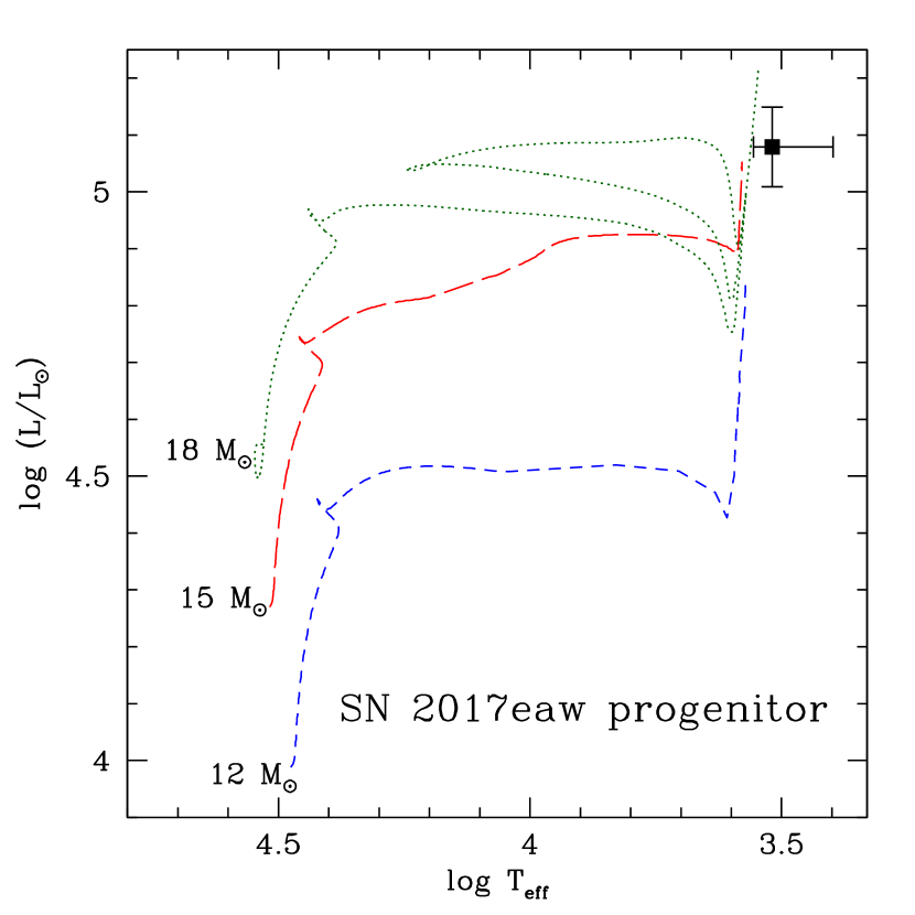
Figure 23: Hertzsprung-Russell diagram showing the locus of the SN 2017eaw progenitor (solid point). Shown for comparison are single-star evolutionary tracks from the Geneva group at subsolar metallicity $Z=0.006$ (with rotation at $\Omega/\Omega_{\rm crit}=0.3$; Georgy et al. 2013) for 12 $M_{\odot}$ (blue short-dashed line) and 15 $M_{\odot}$ (red long-dashed line), and from PARSEC (Bressan et al. 2012; Chen et al. 2015) at $Z=0.010$ for 18 $M_{\odot}$ (dark green dotted line).

None of these tracks provides a particularly satisfactory comparison with the locus for the progenitor. The tracks all appear to terminate (at the initiation of carbon burning for PARSEC, at the end of C burning for Geneva) at warmer $T_{\rm eff}$ than what we infer for the star itself. Conversely, the results from our modeling of the progenitor SED in Section 7.3 might also be too cool, although, as mentioned before, to within the uncertainties of the modeling the trend of the best fits is definitely toward cooler $T_{\rm eff}$. Nevertheless, as one can see, the $T_{\rm eff}$ and $L_{\rm bol}$ for the progenitor are most consistent, to within the 1$\sigma$ uncertainties, with the endpoint of the RSG phase for the 15 $M_{\odot}$ track. At the 1$\sigma$ level the tracks with $M_{\rm ini}=12\ M_{\odot}$ and with $M_{\rm ini}=18\ M_{\odot}$ appear to be ruled out. We therefore conclude that the SN 2017eaw progenitor likely arose from a star with $M_{\rm ini}\approx 15\ M_{\odot}$. Note that this is larger than the $13\ M_{\odot}$ that Van Dyk et al. (2017) estimated, based on a cursory comparison with an RSG photospheric SED, without the inclusion of circumstellar dust, and also assuming a shorter distance to the host galaxy. Assuming $T_{\rm eff}=3300$ K, with $L_{\rm bol}$ we further estimate that the effective radius of the RSG progenitor within approximately a year of explosion was $R_{\rm eff}=1046\pm 90\ R_{\odot}$. This radius, for instance, is larger than what Dessart et al. (2013) derived for the radius of the Type II-P SN 1999em.

8 Discussion and Conclusions

We have presented extensive optical photometric and spectroscopic monitoring of SN 2017eaw from about 4 to 482 days after explosion. We also independently confirmed the TRGB distance estimate to the host galaxy, NGC 6946, $7.73{\pm}0.78$ Mpc (see also Murphy et al. 2018 and Anand et al. 2018). This distance is corroborated by both our SCM and EPM distance estimates based on SN 2017eaw — $7.32\pm 0.60$ and $7.27\pm 0.42$ Mpc, respectively. Eldridge & Xiao (2019) have also endorsed this larger distance to NGC 6946. The extinction to SN 2017eaw appears to be primarily the result of appreciable Galactic foreground dust, consistent with expectations for the host galaxy being at low Galactic latitude. SN 2017eaw is a normal SN II-P, possibly intermediate in both photometric and spectral properties between other SNe II-P, such as SN 1999em, SN 1999gi, and SN 2012aw, and SN 2004et, which also occurred in NGC 6946. We estimated that a nickel mass $M_{\rm Ni}\approx 0.07\ M_{\odot}$ was synthesized in the explosion. Also, the metallicity at the SN site is likely to be subsolar.

We concluded that SN 2017eaw arose from a luminous ($L_{\rm bol}\approx 10^{5.1}\ L_{\odot}$), massive, and cool ($T_{\rm eff}\approx 2500$–3300 K) RSG. The progenitor was surrounded by extended CSM with substantial dust that was established by mass loss during previous stages of stellar evolution, especially during the RSG phase. From detailed, realistic modeling of the observed SED for the progenitor star in 2016 (derived from combined HST and Spitzer data) and comparison of the inferred location of the progenitor in the H-R diagram with recent, state-of-the-art theoretical massive-star evolutionary tracks, we found that the star is consistent with an initial mass of $15\ M_{\odot}$.

Such a high mass for the progenitor is also supported by comparison of the late-time spectra of SN 2017eaw with existing models produced to analyze SN 2004et (Jerkstrand et al. 2012): these nebular spectra are more consistent with the model for an $M_{\rm ini}=15\ M_{\odot}$ progenitor than a $12\ M_{\odot}$ one, whereas a model with even higher mass, at $19\ M_{\odot}$, also appears to be ruled out. We note that both Kilpatrick & Foley (2018) and Rui et al. (2019) concluded that the progenitor initial mass was nearer 12–$13\ M_{\odot}$, although both studies had assumed a shorter distance to the host galaxy.

This case of SN 2017eaw represents an unprecedented photometric characterization, in terms of wavelength coverage, for the progenitor of an SN of any type, especially at this distance. Such coverage has allowed us to model the progenitor SED with the sort of detail normally reserved for RSGs within (for example) the Local Group. It is especially rare to have datapoints in the Spitzer bands. It is by virtue of the star’s high luminosity and infrared excess that this was possible. If we had had, as is usually the situation, only HST F606W and F814W data available, we would have attempted to fit a 3300 K model atmosphere with spherical geometry for a $15\,M_{\odot}$ star from (for example) MARCS (Gustafsson et al. 2008) — without any knowledge of the need for additional CSM extinction — which would have overpredicted somewhat the brightness at F606W. (No atmosphere models at a cooler 3200 K are available from MARCS for a $15\,M_{\odot}$ star, only for a $5\,M_{\odot}$ one.) We would have then assumed the bolometric correction for this temperature at solar metallicity from Levesque et al. (2005; $BC_{V}=-3.66$ mag) and applied that to the $V$ magnitude inferred from the model 3300 K atmosphere — 25.90 mag, when fixing the model SED to the dereddened observed F814W magnitude. This would have resulted in a lower overall luminosity $L_{\rm bol}\approx 10^{4.8}\,L_{\odot}$. Assuming the lower-metallicity $BC_{V}$ from Levesque et al. (2006; $-3.26$ mag), the luminosity would be an even lower $L_{\rm bol}\approx 10^{4.6}\,L_{\odot}$. Even assuming the $BC$ to F814W from Davies & Beasor (2018; 0.0 mag), we would have arrived at $L_{\rm bol}\approx 10^{4.7}\,L_{\odot}$. All of these would have greatly underestimated the actual likely $L_{\rm bol}$ of the progenitor, and subsequently its initial mass: based on the Geneva models alone, $M_{\rm ini}$ would only be $\sim 10$–$11\,M_{\odot}$. This should provide a cautionary tale with respect to deriving the initial masses of SN II-P RSG progenitors, especially of nominally higher luminosity, based on the typically limited datasets available so far for most cases. It would, of course, be inordinately valuable to obtain better wavelength coverage in the future of nearby potential SN hosts, especially in the near- to mid-infrared.

This high range of initial mass for the SN 2017eaw progenitor pushes up against, but does not entirely exceed, the previously established upper limit for SN II-P progenitor initial masses (Smartt et al. 2009; Smartt 2015). This limit remains to be challenged. We expect such massive stars to have extensive wind-driven, dusty mass loss as an RSG (e.g., Massey et al. 2005), although we note that the inferred mass range for the SN 2017eaw progenitor is less than the threshold ($\sim 18\ M_{\odot}$) at which pulsationally driven superwinds are predicted to be prevalent (Yoon & Cantiello 2010). Whether late-stage, pre-explosion outbursts occur for RSGs (Quataert & Shiode 2012; Shiode & Quataert 2014; Fuller 2017) remains to be confirmed observationally. Such a pre-explosion outburst in the case of SN 2017eaw cannot be entirely ruled out observationally (see, e.g., Tinyanont et al. 2019).

It is interesting to contemplate whether SN 2004et, also in NGC 6946, with its higher luminosity might have arisen from a more massive progenitor than SN 2017eaw (see, e.g., Faran et al. 2014). That the two are fortuitously in the same host galaxy makes such a comparison that much more straightforward and compelling. The nature of the progenitor of SN 2004et has been up for debate, with much of the uncertainty arising from detection of the star in ground-based data with limited wavelength coverage: Li et al. (2005) concluded that the progenitor had $M_{\rm ini}=15^{+5}_{-2}\ M_{\odot}$, whereas a revisit by Crockett et al. (2011) resulted in an estimate of $8^{+5}_{-1}\,M_{\odot}$ (the former study assumed a distance of 5.5 Mpc, and the latter, 5.7 Mpc); Jerkstrand et al. (2012; also adopting 5.5 Mpc), based on the modeling of the nebular spectra mentioned above, found the progenitor to be more consistent with $15\ M_{\odot}$; and Maund (2017), based on the SN 2004et stellar environment, estimated that $M_{\rm ini}=17\pm 2\ M_{\odot}$ (with distance assumed at 4.9 Mpc). Eldridge & Xiao (2019) also argued for a larger initial mass for the SN 2004et progenitor. Based on the comparison with SN 2017eaw it now seems more credible that the higher mass estimate applies for SN 2004et.

It is notable that the SN 2017eaw progenitor mass estimates by Kilpatrick & Foley (2018), Rui et al. (2019), and us are all substantially larger than that inferred by Williams et al. (2018; $8.8^{+2.0}_{-0.2}\ M_{\odot}$) from the properties of the stellar environment around the SN. Such low progenitor masses have been generally found for subluminous SNe II-P, and no indication exists that SN 2017eaw is subluminous; in fact, just the opposite seems more plausible. The low mass estimate based on the stellar environment is consistent with the progenitor being relatively spatially isolated (see Figure 20). The origin of this isolation for such a massive star is curious.

It is, of course, necessary to revisit SN 2017eaw when it has significantly faded, particularly at F814W and the WFC3/IR bands with HST or with JWST, to determine whether the candidate progenitor has vanished. One could also reimage the site with Spitzer, although if ejecta dust is forming, as Rho et al. 2018 have found, the SN may not be fading as rapidly; also, opportunities to observe with Spitzer are drawing to a close. We cannot rule out that the light curves may flatten at late times, as a result of SN ejecta-CSM interaction or a light echo off pre-existing circumstellar dust, as in the case of SN 2004et (Kotak et al. 2009; Fabbri et al. 2011). Thus, one of these possibilities may, in fact, be in effect, in which case our wait time may be extended for several years. Nonetheless, we already consider it very unlikely that a less luminous RSG, or even a bluer star, may have been hidden in the glare of the candidate progenitor and be responsible for the SN. None of the observed properties of SN 2017eaw is consistent with an origin as a low-luminosity RSG, or as a blue or yellow star. We therefore fully expect that the candidate progenitor will no longer be at the SN site. (However, we certainly believe it would be worthwhile to place constraints on the existence of a less luminous companion.) We remain confident that the star we have identified will turn out to have been the SN 2017eaw progenitor. Finally, given the inferred lack of interstellar dust internal to the host galaxy at the SN site, we consider it unlikely that SN 2017eaw will have resulted in a detectable extended, interstellar light echo (as is the case, e.g., for SN 2012aw; Van Dyk et al. 2015).

References

- Adams et al. (2017) Adams, S. M., Kochanek, C. S., Gerke, J. R., et al. 2017, MNRAS, 468, 4968
- Anand et al. (2018) Anand, G. S., Rizzi, L., & Tully, R. B. 2018, AJ, 156, 105
- Anderson et al. (2014) Anderson, J. P., González-Gaitán, S., Hamuy, M., et al. 2014, ApJ, 786, 67
- Arnett & Fu (1989) Arnett, W. D., & Fu, A. 1989, ApJ, 340, 396
- Asplund et al. (2009) Asplund, M., Grevesse, N., Sauval, A. J., et al. 2009, ARA&A, 47, 481
- Baron et al. (1994) Baron, E., Hauschildt, P. H., & Branch, D. 1994, ApJ, 426, 334
- Belley & Roy (1992) Belley, J., & Roy, J.-R. 1992, ApJS, 78, 61
- Bersten & Hamuy (2009) Bersten, M. C., & Hamuy, M. 2009, ApJ, 701, 200
- Bertin & Arnouts (1996) Bertin, E., & Arnouts, S. 1996, A&AS, 117, 393
- Bertin et al. (2002) Bertin, E., Mellier, Y., Radovich, M., et al. 2002, in ASP Conf. Ser. 281, Astronomical Data Analysis Software and Systems XI, ed. D. A. Bohlender, D. Durand, & T. H. Handley (San Francisco, CA: ASP), 228
- Blondin & Tonry (2007) Blondin, S., & Tonry, J. L. 2007, ApJ, 666, 1024
- Bose & Kumar (2014) Bose, S., & Kumar, B. 2014, ApJ, 782, 98
- Bose et al. (2013) Bose, S., Kumar, B., Sutaria, F., et al. 2013, MNRAS, 433, 1871
- Botticella et al. (2009) Botticella, M. T., Pastorello, A., Smartt, S. J., et al. 2009, MNRAS, 398, 1041
- Bottinelli et al. (1984) Bottinelli, L., Gouguenheim, L., Paturel, G., et al. 1984, A&AS, 56, 381
- Bottinelli et al. (1986) Bottinelli, L., Gouguenheim, L., Paturel, G., et al. 1986, A&A, 156, 157
- Bressan et al. (2012) Bressan, A., Marigo, P., Girardi, L., et al. 2012, MNRAS, 427, 127
- Bruursema et al. (2014) Bruursema, J., Meixner, M., Long, K. S., et al. 2014, AJ, 148, 41
- Cardelli et al. (1989) Cardelli, J. A., Clayton, G. C., & Mathis, J. S. 1989, ApJ, 345, 245
- Chen et al. (2015) Chen, Y., Bressan, A., Girardi, L., et al. 2015, MNRAS, 452, 1068
- Cheng et al. (2017) Cheng, Y.-C., Chen, T.-W., & Prentice, S. 2017, ATel, 10374, 1
- Crockett et al. (2011) Crockett, R. M., Smartt, S. J., Pastorello, A., et al. 2011, MNRAS, 410, 2767
- Dall’Ora et al. (2014) Dall’Ora, M., Botticella, M. T., Pumo, M. L., et al. 2014, ApJ, 787, 139
- Davies & Beasor (2018) Davies, B., & Beasor, E. R. 2018, MNRAS, 474, 2116
- Davies et al. (2013) Davies, B., Kudritzki, R.-P., Plez, B., et al. 2013, ApJ, 767, 3
- De Beck et al. (2010) De Beck, E., Decin, L., de Koter, A., et al. 2010, A&A, 523, A18
- Dessart & Hillier (2005) Dessart, L., & Hillier, D. J. 2005, A&A, 439, 671
- Dessart et al. (2013) Dessart, L., Hillier, D. J., Waldman, R., et al. 2013, MNRAS, 433, 1745
- Dolphin (2000) Dolphin, A. E. 2000, PASP, 112, 1383
- Dolphin (2016) Dolphin, A. 2016, DOLPHOT: Stellar photometry, ascl:1608.013
- Dong & Stanek (2017) Dong, S., & Stanek, K. Z. 2017, ATel, 10372, 1
- Draine & Lee (1984) Draine, B. T., & Lee, H. M. 1984, ApJ, 285, 89
- Drake et al. (2017) Drake, A. J., Djorgovski, S. G., Mahabal, A. A., et al. 2017, ATel, 10397, 1
- Eastman & Kirshner (1989) Eastman, R. G., & Kirshner, R. P. 1989, ApJ, 347, 771
- Eldridge & Xiao (2019) Eldridge, J. J., & Xiao, L. 2019, MNRAS, 485, L58
- Elmhamdi et al. (2003a) Elmhamdi, A., Chugai, N. N., & Danziger, I. J. 2003a, A&A, 404, 1077
- Elmhamdi et al. (2003b) Elmhamdi, A., Danziger, I. J., Chugai, N., et al. 2003b, MNRAS, 338, 939
- Fabbri et al. (2011) Fabbri, J., Otsuka, M., Barlow, M. J., et al. 2011, MNRAS, 418, 1285
- Faran et al. (2018) Faran, T., Nakar, E., & Poznanski, D. 2018, MNRAS, 473, 513
- Faran et al. (2014) Faran, T., Poznanski, D., Filippenko, A. V., et al. 2014, MNRAS, 442, 844
- Fazio et al. (2004) Fazio, G. G., Hora, J. L., Allen, L. E., et al. 2004, ApJS, 154, 10
- Filippenko (1982) Filippenko, A. V. 1982, PASP, 94, 715
- Filippenko et al. (2001) Filippenko, A. V., Li, W. D., Treffers, R. R., & Modjaz, M. 2001, in ASP Conf. Ser., Vol. 246, IAU Colloq. 183, Small Telescope Astronomy on Global Scales (San Francisco, CA: ASP), 121
- Förster et al. (2018) Förster, F., Moriya, T. J., Maureira, J. C., et al. 2018, Nature Astronomy, 2, 808
- Fraser et al. (2012) Fraser, M., Maund, J. R., Smartt, S. J., et al. 2012, ApJ, 759, L13
- Fraser et al. (2014) Fraser, M., Maund, J. R., Smartt, S. J., et al. 2014, MNRAS, 439, L56
- Fuller (2017) Fuller, J. 2017, MNRAS, 470, 1642
- Gal-Yam et al. (2014) Gal-Yam, A., Arcavi, I., Ofek, E. O., et al. 2014, Nature, 509, 471
- Ganeshalingam et al. (2010) Ganeshalingam, M., Li, W., Filippenko, A. V., et al. 2010, ApJS, 190, 418
- Garnavich et al. (2016) Garnavich, P. M., Tucker, B. E., Rest, A., et al. 2016, ApJ, 820, 23
- Georgy (2012) Georgy, C. 2012, A&A, 538, L8
- Georgy et al. (2013) Georgy, C., Ekström, S., Granada, A., et al. 2013, A&A, 553, A24
- Gusev et al. (2013) Gusev, A. S., Sakhibov, F. H., & Dodonov, S. N. 2013, Astrophysical Bulletin, 68, 40
- Gustafsson et al. (2008) Gustafsson, B., Edvardsson, B., Eriksson, K., et al. 2008, A&A, 486, 951
- Gutiérrez et al. (2017) Gutiérrez, C. P., Anderson, J. P., Hamuy, M., et al. 2017, ApJ, 850, 89
- Hack et al. (2012) Hack, W. J., Dencheva, N., Fruchter, A. S., et al. 2012, American Astronomical Society Meeting Abstracts #220, 220, 135.15
- Hamuy & Pinto (2002) Hamuy, M., & Pinto, P. A. 2002, ApJ, 566, L63
- Hamuy et al. (2001) Hamuy, M., Pinto, P. A., Maza, J., et al. 2001, ApJ, 558, 615
- Hardy et al. (2015) Hardy, L. K., Butterley, T., Dhillon, V. S., et al. 2015, MNRAS, 454, 4316
- Harutyunyan et al. (2008) Harutyunyan, A. H., Pfahler, P., Pastorello, A., et al. 2008, A&A, 488, 383
- Howard et al. (2010) Howard, A. W., Johnson, J. A., Marcy, G. W., et al. 2010, ApJ, 721, 1467
- Huang et al. (2018) Huang, F., Wang, X.-F., Hosseinzadeh, G., et al. 2018, MNRAS, 475, 3959
- Hyman et al. (1995) Hyman, S. D., Van Dyk, S. D., Weiler, K. W., et al. 1995, ApJ, 443, L77
- Indebetouw et al. (2005) Indebetouw, R., Mathis, J. S., Babler, B. L., et al. 2005, ApJ, 619, 931
- James & Baron (2010) James, S., & Baron, E. 2010, ApJ, 718, 957
- Jang et al. (2018) Jang, I. S., Hatt, D., Beaton, R. L., et al. 2018, ApJ, 852, 60
- Jang & Lee (2017) Jang, I. S., & Lee, M. G. 2017, ApJ, 835, 28
- Jarrett et al. (2003) Jarrett, T. H., Chester, T., Cutri, R., et al. 2003, AJ, 125, 525
- Jerkstrand et al. (2012) Jerkstrand, A., Fransson, C., Maguire, K., et al. 2012, A&A, 546, A28
- Jerkstrand et al. (2014) Jerkstrand, A., Smartt, S. J., Fraser, M., et al. 2014, MNRAS, 439, 3694
- Johnson et al. (2018) Johnson, S. A., Kochanek, C. S., & Adams, S. M. 2018, MNRAS, 480, 1696
- Karachentsev et al. (2000) Karachentsev, I. D., Sharina, M. E., & Huchtmeier, W. K. 2000, A&A, 362, 544
- Khan (2017) Khan, R. 2017, ATel, 10373, 1
- Khazov et al. (2016) Khazov, D., Yaron, O., Gal-Yam, A., et al. 2016, ApJ, 818, 3
- Kilpatrick & Foley (2018) Kilpatrick, C. D., & Foley, R. J. 2018, MNRAS, 481, 2536
- Kirshner & Kwan (1974) Kirshner, R. P., & Kwan, J. 1974, ApJ, 193, 27
- Kochanek (2019) Kochanek, C. S. 2019, MNRAS, 483, 3762
- Kochanek et al. (2012) Kochanek, C. S., Khan, R., & Dai, X. 2012, ApJ, 759, 20
- Kotak et al. (2009) Kotak, R., Meikle, W. P. S., Farrah, D., et al. 2009, ApJ, 704, 306
- Kučinskas et al. (2005) Kučinskas, A., Hauschildt, P. H., Ludwig, H.-G., et al. 2005, A&A, 442, 281
- Leonard et al. (2002a) Leonard, D. C., Filippenko, A. V., Gates, E. L., et al. 2002a, PASP, 114, 35
- Leonard et al. (2002b) Leonard, D. C., Filippenko, A. V., Li, W., et al. 2002b, AJ, 124, 2490
- Levesque et al. (2005) Levesque, E. M., Massey, P., Olsen, K. A. G., et al. 2005, ApJ, 628, 973
- Levesque et al. (2006) Levesque, E. M., Massey, P., Olsen, K. A. G., et al. 2006, ApJ, 645, 1102
- Li et al. (2011) Li, W., Leaman, J., Chornock, R., et al. 2011, MNRAS, 412, 1441
- Li et al. (2005) Li, W., Van Dyk, S. D., Filippenko, A. V., & Cuillandre, J.-C. 2005, PASP, 117, 121
- Lyman et al. (2014) Lyman, J. D., Bersier, D., & James, P. A. 2014, MNRAS, 437, 3848
- Madore et al. (2009) Madore, B. F., Mager, V., & Freedman, W. L. 2009, ApJ, 690, 389
- Mager et al. (2008) Mager, V. A., Madore, B. F., & Freedman, W. L. 2008, ApJ, 689, 721
- Maguire et al. (2010) Maguire, K., Di Carlo, E., Smartt, S. J., et al. 2010, MNRAS, 404, 981
- Makovoz & Khan (2005) Makovoz, D., & Khan, I. 2005, in ASP Conf. Ser. 347, Astronomical Data Analysis Software and Systems XIV, ed. P. Shopbell, M. Britton, & R. Ebert (San Francisco, CA: ASP), 81
- Makovoz & Marleau (2005) Makovoz, D., & Marleau, F. R. 2005, PASP, 117, 1113
- Makovoz et al. (2006) Makovoz, D., Roby, T., Khan, I., et al. 2006, Proc. SPIE, 6274, 62740C
- Massey et al. (2005) Massey, P., Plez, B., Levesque, E. M., et al. 2005, ApJ, 634, 1286
- Matonick & Fesen (1997) Matonick, D. M., & Fesen, R. A. 1997, ApJS, 112, 49
- Maund et al. (2014a) Maund, J. R., Mattila, S., Ramirez-Ruiz, E., & Eldridge, J. J. 2014a, MNRAS, 438, 1577
- Maund et al. (2014b) Maund, J. R., Reilly, E., & Mattila, S. 2014b, MNRAS, 438, 938
- Maund (2017) Maund, J. R. 2017, MNRAS, 469, 2202
- Maund & Smartt (2009) Maund, J. R., & Smartt, S. J. 2009, Science, 324, 486
- Milisavljevic et al. (2012) Milisavljevic, D., Fesen, R. A., Chevalier, R. A., et al. 2012, ApJ, 751, 25
- Milisavljevic et al. (2013) Milisavljevic, D., Margutti, R., Soderberg, A. M., et al. 2013, ApJ, 767, 71
- Miller & Stone (1993) Miller, J. S., & Stone, R. P. S. 1993, Lick Obs. Tech. Rep. No. 66
- Misra et al. (2007) Misra, K., Pooley, D., Chandra, P., et al. 2007, MNRAS, 381, 280
- Modjaz et al. (2011) Modjaz, M., Kewley, L., Bloom, J. S., et al. 2011, ApJ, 731, L4
- Moriya et al. (2018) Moriya, T. J., Förster, F., Yoon, S.-C., et al. 2018, MNRAS, 476, 2840
- Moriya et al. (2017) Moriya, T. J., Yoon, S.-C., Gräfener, G., et al. 2017, MNRAS, 469, L108
- Morozova et al. (2017) Morozova, V., Piro, A. L., & Valenti, S. 2017, ApJ, 838, 28
- Morozova et al. (2018) Morozova, V., Piro, A. L., & Valenti, S. 2018, ApJ, 858, 15
- Murphy et al. (2018) Murphy, J. W., Khan, R., Williams, B., et al. 2018, ApJ, 860, 117
- Nicholl (2018) Nicholl, M. 2018, RNAAS, 2, 230
- Nugent et al. (2006) Nugent, P., Sullivan, M., Ellis, R., et al. 2006, ApJ, 645, 841
- O’Neill et al. (2019) O’Neill, D., Kotak, R., Fraser, M., et al. 2019, A&A, 622, L1
- Olivares E. et al. (2010) Olivares E., F., Hamuy, M., Pignata, G., et al. 2010, ApJ, 715, 833
- Ossenkopf et al. (1992) Ossenkopf, V., Henning, T., & Mathis, J. S. 1992, A&A, 261, 567
- Paxton et al. (2018) Paxton, B., Schwab, J., Bauer, E. B., et al. 2018, The Astrophysical Journal Supplement Series, 234, 34.
- Pejcha & Prieto (2015) Pejcha, O., & Prieto, J. L. 2015, ApJ, 799, 215
- Phillips et al. (2013) Phillips, M. M., Simon, J. D., Morrell, N., et al. 2013, ApJ, 779, 38
- Pierce (1994) Pierce, M. J. 1994, ApJ, 430, 53
- Polshaw et al. (2015) Polshaw, J., Kotak, R., Chambers, K. C., et al. 2015, A&A, 580, L15
- Poznanski et al. (2009) Poznanski, D., Butler, N., Filippenko, A. V., et al. 2009, ApJ, 694, 1067
- Pozzo et al. (2006) Pozzo, M., Meikle, W. P. S., Rayner, J. T., et al. 2006, MNRAS, 368, 1169
- Prieto et al. (2008) Prieto, J. L., Kistler, M. D., Thompson, T. A., et al. 2008, ApJ, 681, L9
- Quataert & Shiode (2012) Quataert, E., & Shiode, J. 2012, MNRAS, 423, L92
- Rho et al. (2018) Rho, J., Geballe, T. R., Banerjee, D. P. K., et al. 2018, ApJ, 864, L20
- Rieke et al. (2004) Rieke, G. H., Young, E. T., Engelbracht, C. W., et al. 2004, ApJS, 154, 25
- Riess et al. (1999) Riess, A. G., Filippenko, A. V., Li, W., et al. 1999, AJ, 118, 2675
- Riess et al. (2016) Riess, A. G., Macri, L. M., Hoffmann, S. L., et al. 2016, ApJ, 826, 56
- Rui et al. (2019) Rui, L., Wang, X., Mo, J., et al. 2019, MNRAS, 485, 1990
- Sahu et al. (2006) Sahu, D. K., Anupama, G. C., Srividya, S., & Muneer, S. 2006, MNRAS, 372, 1315
- Sakai et al. (1999) Sakai, S., Madore, B. F., & Freedman, W. L. 1999, ApJ, 511, 671
- Sakai et al. (2000) Sakai, S., Zaritsky, D., & Kennicutt, R. C. 2000, AJ, 119, 1197
- Sargent et al. (2011) Sargent, B. A., Srinivasan, S., & Meixner, M. 2011, ApJ, 728, 93
- Sawicki (2012) Sawicki, M. 2012, PASP, 124, 1208
- Schlafly & Finkbeiner (2011) Schlafly, E. F., & Finkbeiner, D. P. 2011, ApJ, 737, 103
- Schmidt et al. (1992) Schmidt, B. P., Kirshner, R. P., & Eastman, R. G. 1992, ApJ, 395, 366
- Schmidt et al. (1994) Schmidt, B. P., Kirshner, R. P., Eastman, R. G., et al. 1994, ApJ, 432, 42
- Schoniger & Sofue (1994) Schoniger, F., & Sofue, Y. 1994, A&A, 283, 21
- Shiode & Quataert (2014) Shiode, J. H., & Quataert, E. 2014, ApJ, 780, 96
- Shivvers et al. (2017) Shivvers, I., Zheng, W., Van Dyk, S. D., et al. 2017, MNRAS, 471, 4381
- Silverman et al. (2012) Silverman, J. M., Foley, R. J., Filippenko, A. V., et al. 2012, MNRAS, 425, 1789
- Smartt (2015) Smartt, S. J. 2015, PASA, 32, e016
- Smartt et al. (2009) Smartt, S. J., Eldridge, J. J., Crockett, R. M., & Maund, J. R. 2009, MNRAS, 395, 1409
- Smartt et al. (2004) Smartt, S. J., Maund, J. R., Hendry, M. A., et al. 2004, Science, 303, 499
- Smith et al. (2011) Smith, N., Li, W., Filippenko, A. V., & Chornock, R. 2011, MNRAS, 412, 1522
- Smith et al. (2015) Smith, N., Mauerhan, J. C., Cenko, S. B., et al. 2015, MNRAS, 449, 1876
- Soraisam et al. (2018) Soraisam, M. D., Bildsten, L., Drout, M. R., et al. 2018, ApJ, 859, 73
- Srinivasan et al. (2011) Srinivasan, S., Sargent, B. A., & Meixner, M. 2011, A&A, 532, A54
- Steele & Newsam (2017) Steele, I. A., & Newsam, A. M. 2017, ATel, 10384, 1
- Stetson (1987) Stetson, P. B. 1987, PASP, 99, 191
- Stritzinger et al. (2002) Stritzinger, M., Hamuy, M., Suntzeff, N. B., et al. 2002, AJ, 124, 2100
- STScI Development Team (2013) STScI Development Team 2013, pysynphot: Synthetic photometry software package, Astrophysics Source Code Library, ascl:1303.023
- Sukhbold et al. (2016) Sukhbold, T., Ertl, T., Woosley, S. E., Brown, J. M., & Janka, H.-T. 2016, ApJ, 821, 38
- Suntzeff & Bouchet (1990) Suntzeff, N. B., & Bouchet, P. 1990, AJ, 99, 650
- Takáts & Vinkó (2012) Takáts, K., & Vinkó, J. 2012, MNRAS, 419, 2783
- Thompson et al. (2009) Thompson, T. A., Prieto, J. L., Stanek, K. Z., et al. 2009, ApJ, 705, 1364
- Tikhonov (2014) Tikhonov, N. A. 2014, Astronomy Letters, 40, 537
- Tinyanont et al. (2019) Tinyanont, S., Kasliwal, M. M., Krafton, K., et al. 2019, ApJ, 873, 127
- Tody (1986) Tody, D. 1986, Proc. SPIE, 627, 733
- Tody (1993) Tody, D. 1993, ASP Conf. Ser. 52, Astronomical Data Analysis Software and Systems II, ed. R. J. Hanisch, R. J. V. Brissenden and J. Barnes (San Francisco, CA: ASP), 173
- Tomasella et al. (2017) Tomasella, L., Benetti, S., Cappellaro, E., et al. 2017, ATel, 10377, 1
- Tonry et al. (2012) Tonry, J. L., Stubbs, C. W., Lykke, K. R., et al. 2012, ApJ, 750, 99
- Tsvetkov et al. (2018) Tsvetkov, D. Y., Shugarov, S. Y., Volkov, I. M., et al. 2018, Astronomy Letters, 44, 315
- Ueta & Meixner (2003) Ueta, T., & Meixner, M. 2003, ApJ, 586, 1338
- Valenti et al. (2016) Valenti, S., Howell, D. A., Stritzinger, M. D., et al. 2016, MNRAS, 459, 3939
- Van Dyk (2017) Van Dyk, S. D. 2017, RSPTA, 375, 20160277
- Van Dyk et al. (2012a) Van Dyk, S. D., Cenko, S. B., Poznanski, D., et al. 2012a, ApJ, 756, 131
- Van Dyk et al. (2012b) Van Dyk, S. D., Davidge, T. J., Elias-Rosa, N., et al. 2012b, AJ, 143, 19
- Van Dyk et al. (2017) Van Dyk, S. D., Filippenko, A. V., Fox, O. D., et al. 2017, ATel, 10378, 1
- Van Dyk et al. (2015) Van Dyk, S. D., Lee, J. C., Anderson, J., et al. 2015, ApJ, 806, 195
- Van Dyk et al. (2003) Van Dyk, S. D., Li, W., & Filippenko, A. V. 2003, PASP, 115, 1289
- van Loon (2006) van Loon, J. T. 2006, in ASP Conf. Ser. 353, Stellar Evolution at Low Metallicity: Mass Loss, Explosions, Cosmology, ed. H. J. G. L. M. Lamers et al. (San Francisco, CA: ASP), 211
- Vogl et al. (2019) Vogl, C., Sim, S. A., Noebauer, U. M., et al. 2019, A&A, 621, A29
- Vogt et al. (1994) Vogt, S. S., Allen, S. L., Bigelow, B. C., et al. 1994, in Proc. SPIE, Vol. 2198, Instrumentation in Astronomy VIII, ed. D. L. Crawford & E. R. Craine, 362
- Walmswell & Eldridge (2012) Walmswell, J. J., & Eldridge, J. J. 2012, MNRAS, 419, 2054
- Wiggins (2017) Wiggins, P. 2017, Transient Name Server Discovery Report, 548
- Williams et al. (2018) Williams, B. F., Hillis, T. J., Murphy, J. W., et al. 2018, ApJ, 860, 39
- Williams et al. (2014) Williams, B. F., Peterson, S., Murphy, J., et al. 2014, ApJ, 791, 105
- Xiang et al. (2017) Xiang, D., Rui, L., Wang, X., et al. 2017, ATel, 10376, 1
- Yaron & Gal-Yam (2012) Yaron, O., & Gal-Yam, A. 2012, PASP, 124, 668
- Yoon & Cantiello (2010) Yoon, S.-C., & Cantiello, M. 2010, ApJ, 717, L62
- Zhang & Wang (1996) Zhang, Q., & Wang, Z. R. 1996, A&A, 307, 166