Variational Inference of Joint Models using Multivariate Gaussian Convolution Processes

Abstract

We present a non-parametric prognostic framework for individualized event prediction based on joint modeling of both longitudinal and time-to-event data. Our approach exploits a multivariate Gaussian convolution process (MGCP) to model the evolution of longitudinal signals and a Cox model to map time-to-event data with longitudinal data modeled through the MGCP. Taking advantage of the unique structure imposed by convolved processes, we provide a variational inference framework to simultaneously estimate parameters in the joint MGCP-Cox model. This significantly reduces computational complexity and safeguards against model overfitting. Experiments on synthetic and real world data show that the proposed framework outperforms state-of-the art approaches built on two-stage inference and strong parametric assumptions.

1 Introduction

In recent years, the multivariate Gaussian process (MGP) has drawn significant attention as an efficient non-parametric approach to predict longitudinal signal trajectories (Dürichen et al., 2015; Moreno-Muñoz et al., 2018; Kontar et al., 2018b). The MGP draws its roots from multitask learning where transfer of knowledge is achieved through a shared representation between training and testing signals. One neat approach that achieves this knowledge transfer, employs convolution processes to construct the MGP. Specifically, each signal is expressed as a convolution of latent functions drawn from a Gaussian process (GP). Commonalities amongst training and testing signals are then captured by sharing these latent functions across the outputs (Titsias & Lawrence, 2010; Álvarez et al., 2010; Álvarez & Lawrence, 2011). Consequently, the multiple signals can be expressed as a single output from a common multivariate Gaussian convolution process (MGCP). Indeed, many recent studies have demonstrated the MGCP ability to account for non-trivial commonalities in the data and provide accurate predictive results (Zhao & Sun, 2016; Guarnizo & Álvarez, 2018; Cheng, 2018).

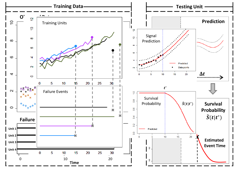
Figure 1: Joint modeling of longitudinal and time-to-event data.

In this article we exploit the MGCP to explore the following question: can we use both time-to-event data (also known as survival data) along with longitudinal signals to obtain a reliable event prediction? This is illustrated in Figure 1. As shown in the figure, our goal is to utilize both survival data and longitudinal signals from training units to predict the survival probability of a partially observed testing unit. Naturally, the aforementioned question is often encountered in a wide range of applications, including: disease prognosis in clinical trials, event prediction using vital health signals from monitored patients at risk, remaining useful life estimation of operational units/machines and failure prognosis in connected manufacturing systems (e.g., nuclear power plants) (Tsiatis et al., 1995; Bycott & Taylor, 1998; Gasmi et al., 2003; Pham et al., 2012; Gao et al., 2015; Soleimani et al., 2018).

In order to link survival and longitudinal data, state-of-the-art methods have focused on joint models. The seminal work of Rizopoulos (Rizopoulos, 2011, 2012) laid a foundation for joint models where a linear mixed effects model is used to model longitudinal signals. The coefficients of the mixed model are then used in a Cox model to compute the probability of event occurrence conditioned on the observed longitudinal signals. This idea provided the bases for many extensions and applications in the literature (Crowther et al., 2012; Wu et al., 2012; Zhu et al., 2012; Crowther et al., 2013; Proust-Lima et al., 2014; He et al., 2015; Rizopoulos et al., 2017; Mauff et al., 2018). It is important to note here that joint methods are in general built using a two-stage inference procedure. In two-stage inference, features from the longitudinal data are first learned, these estimated features are then inserted into a survival model to predict event probabilities. Indeed, many papers have shown that this two-stage procedure can produce competitive predictive results (Wulfsohn & Tsiatis, 1997; Yu et al., 2004; Zhou et al., 2014; Mauff et al., 2018). Nevertheless, the foregoing works are based on strong parametric assumptions where signals are assumed to follow a specific parametric form and all the signals (training and testing) exhibit that same functional form. In other words, signals behave according to a similar trend but at different rates (i.e., different parameter values). However, parametric methods are restrictive in many applications and if the specified form is far from the truth, predictive results will be misleading. Furthermore, the assumption that all signals possess the same functional form may not hold in real-life applications. For instance, units operated under different environmental conditions may exhibit different signal evolution rates and trends (Yan et al., 2016; Kontar et al., 2018a). Some recent efforts aimed to relax strong parametric assumptions using splines, continuous time Markov chains and the GP. Unfortunately, these methods still assume homogeneity across the population and focus on merely imputing the longitudinal data rather than predicting signal evolution within a time interval of interest (Dempsey et al., 2017; Soleimani et al., 2018). We here note that there has been some recent attempts at rebuilding the Cox model using a GP (Fernández et al., 2016; Kim & Pavlovic, 2018). However these approaches are only based on survival data and do not handle joint modeling, which is the focus of this article.

To address the aforementioned challenges, we propose a flexible joint modeling approach denoted as MGCP-Cox. Our approach exploits the MGCP to model the evolution of longitudinal signals and a Cox model to map time-to-event data with longitudinal data modeled through MGCP. Event occurrence probability is then derived within any future interval $\Delta t$ as shown in Figure 1. We also propose a variational inference framework using pseudo-inputs (Snelson & Ghahramani, 2006; Damianou & Lawrence, 2013) to simultaneously estimate parameters in the joint MGCP-Cox model. This facilitates scalability to large data settings and safeguards against model overfitting. Finally, the advantageous features of the proposed method are demonstrated through numerical studies and a case study with real-world data in the application to finding the remaining useful lifetime of NASA Aero-propulsion engines.

The rest of the paper is organized as follows. In section 2 we briefly review survival analysis. In section 3, we present our joint modeling framework and the variational inference algorithm. Numerical experiments using synthetic data and real-world data are provided in section 4. Finally, section 5 concludes the paper with a brief discussion. A detailed code and the used real-world data are available in the supplementary materials.

2 Background: Survival Analysis

In this section, we will briefly review survival analysis which will be used for event prediction in the joint model. Survival analysis is a branch of statistics for analyzing time-to-event data and predicting the probability of occurrence of an event. For each individual unit $i$, the associated data is $\bm{\bm{\mathcal{D}}}_{i}=(V_{i},\delta_{i},\bm{Y}_{i},\bm{w}_{i})$, where $V_{i}=\min\{T_{i},C_{i}\}$ is the event time (the unit failed at time $T_{i}$ or was censored at time $C_{i}$), $\delta_{i}\in\{0,1\}$ is an event indicator ($\delta_{i}=1/0$ indicates the unit has failed/censored), $\bm{Y}_{i}$ are the noisy observed longitudinal data (e.g., vital signals collected from patients) corresponding to the underlying latent values $\bm{f}_{i}$, and $\bm{w}_{i}$ is a set of time-invariant features (e.g., patient’s gender). Typically, the continuous random variable $T_{i}$ is characterized by a survival function $S(t)=P(T\geq t)$ which represents the probability of survival up to time $t$. Another important term is the hazard function $h(t)=\lim_{\Delta\to 0}\frac{1}{\Delta}P(t<T\leq t+\Delta|T\geq t)=-\frac{d}{dt}\log S(t)$ and can be thought of as the instantaneous rate of occurrence of an event at time $t$. It is easy to show that $S(t)=\exp\{-\int_{0}^{t}h(u)du\}$. The term $\int_{0}^{t}h(u)du$ is called cumulative hazard function and is denoted by $H(t)$. The basic scheme of survival analysis is to find suitable models to explain relationships between the hazard function $h_{i}(t)$ and collected data $\bm{\mathcal{D}}_{i}$. These models are defined as survival models.

Many survival models have been developed to analyze time-to-event data. They typically model the hazard function as a function of some time-varying and fixed features. One class of prevailed survival models is called the Cox model (Cox, 1972), which has the form $h_{i}(t)=h_{0}(t)\exp[\bm{\gamma}^{T}\bm{w}_{i}+\beta f_{i}(t)]$, where $h_{0}(t)$ is a baseline hazard function shared by all individuals, and is typically modeled by the Weibull or a piecewise constant function, $\bm{\gamma}$ is a vector of coefficients for the fixed covariates (features), $f_{i}(t)$ is the feature estimated by a longitudinal model (e.g., linear mixed model, Gaussian Process), and $\beta$ is a scaling parameter for the time-varying covariates. Parameters in the Cox model are typically estimated by maximizing the log-likelihood function

$$\begin{split}&\sum_{i=1}^{N}\log p(V_{i},\delta_{i}|\bm{w}_{i},\bm{f}_{i})\\ &=\sum_{i=1}^{N}\{\delta_{i}\log\big{[}h_{0}(V_{i})\exp[\bm{\gamma}^{T}\bm{w}_{i}+\beta f_{i}(V_{i})]\big{]}\\ &-\int_{0}^{V_{i}}h_{0}(u)\exp[\bm{\gamma}^{T}\bm{w}_{i}+\beta f_{i}(u)]du\}.\end{split}$$ (1)

For a comprehensive review of survival models, see (Kalbfleisch & Prentice, 2011). Given an estimate of parameters from the Cox model, we can then obtain the event (failure) probability within a future time interval $\Delta t$ given the fact that the testing unit $i$ survives non-shorter than the current time instance $t^{*}$. This probability, denoted $\hat{P}_{\Delta t}$, is estimated as follows:

$$\begin{split}&\hat{P}_{\Delta t}=1-\hat{S}(t^{*}+\Delta t|t^{*},\bm{w}_{i},\bm{f}_{i})=1-\frac{\hat{S}(t^{*}+\Delta t|\bm{w}_{i},\bm{f}_{i})}{\hat{S}(t^{*}|\bm{w}_{i},\bm{f}_{i})}\\ &=1-\exp\big{\{}-\int_{t^{*}}^{t^{*}+\Delta t}\hat{h}_{0}(u)\exp\big{[}\bm{\hat{\gamma}}^{T}\bm{w}_{i}+\hat{\beta}f_{i}(u)\big{]}du\big{\}},\end{split}$$ (2)

where $\bm{w}_{i}$ and $\bm{f}_{i}$ are features for a testing unit $i$. Note that in Figure 1 we show the survival curve which is defined as $\hat{S}(t|t^{\ast})=1-\hat{P}_{\Delta t}$ , where $t=t^{*}+\Delta t$.

3 Joint Modeling and Variational Inference

3.1 The multivariate Gaussian convolution process (MGCP)

Assume data have been collected from $N$ units and let $\mathcal{I}=\{1,2,\ldots,N\}$ denote the set of all units. For unit $i$, its associated data is $\bm{\bm{\mathcal{D}}}_{i}=\{V_{i},\delta_{i},\bm{Y}_{i},\bm{w}_{i}\}$. The observed longitudinal signal is denoted by $\bm{Y}_{i}=(y_{i}(t_{i1}),\ldots,y_{i}(t_{il_{i}}))^{T}$, where $l_{i}$ represents the number of observations and $\{t_{ir}:r=1,\ldots,l_{i}\}$ denotes the inputs. We decompose the longitudinal signal as $y_{i}(t)=f_{i}(t)+\epsilon_{i}(t)$, where $f_{i}(\cdot)$ is a mean zero GP and $\epsilon_{i}(t)$ denotes additive noise with zero mean and $\sigma_{\epsilon}^{2}$ variance.

To obtain an accurate predictive result, we need to capture the intrinsic relatedness among $N$ signals. Particularly, we resort to the convolution process to model the latent function $f_{i}(t)$. We consider $K$ independent latent functions $\{X_{k}(t)\}_{k=1}^{K}$ and $NK$ different smoothing kernels $\{G_{i,k}(t):i\in\mathcal{I}\}_{k=1}^{K}$. The latent functions are assumed independent GPs with covariance $\mbox{cov}[X_{k}(t),X_{k}(t^{\prime})]=\kappa_{k}(t,t^{\prime})$. We set $G_{i,k}(t)=\alpha_{i,k}\mathcal{N}(0,\xi_{i,k}^{2})$ to be scaled Gaussian kernels and $\kappa_{k}(t,t^{\prime})$ to be squared exponential covariance functions (Álvarez & Lawrence, 2009).

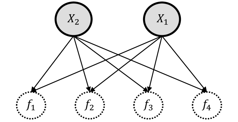
Figure 2: Illustration of a convolution Process where two latent functions $X_{1},X_{2}$ are shared across four outputs.

$$\begin{split}&\kappa_{k}(t,t^{\prime})=\exp\bigg{[}-\frac{1}{2}\frac{(t-t^{\prime})^{2}}{\lambda_{k}^{2}}\bigg{]}\\ &=\sqrt{2\pi\lambda_{k}^{2}}\mathcal{N}(0,\lambda_{k}^{2})\coloneqq C_{k}\mathcal{N}(0,\lambda_{k}^{2}),\end{split}$$ (3)

The GP $f_{i}(t)$ is then constructed by convolving the shared latent functions with the smoothing kernel as shown in (4). This is the underlying principle of the MGCP, where the latent functions $\{X_{k}(t)\}_{k=1}^{K}$ are shared across different outputs through the corresponding kernels $G_{i,k}(t)$. Since convolutions are linear operators on a function and since the latent function, a GP, is shared across multiple outputs then all outputs can be expressed as a jointly distributed GP, an MGCP. As shown in Figure 2, a key feature is that information is shared through different parameters encoded in the kernels $G_{i,k}(t)$. Outputs then can possess both shared and unique features. Thus, accounting for heterogeneity in the longitudinal data.

$$f_{i}(t)=\sum_{k=1}^{K}\int_{\mathbb{R}}G_{i,k}(t-u)X_{k}(u)du.$$ (4)

Based on equation (4), the covariance function between $f_{i}$ and $f_{j}$, and the covariance function between $f_{i}$ and $X_{k}$, can be calculated as

$$\begin{split}&\kappa_{f_{i},f_{j}}(t,t^{\prime})\\ &=\sum_{k=1}^{K}\int_{\mathbb{R}}G_{i,k}(t-u)\int_{\mathbb{R}}G_{j,k}(t^{\prime}-u^{\prime})\kappa_{k}(u,u^{\prime})du^{\prime}du\\ &=\sum_{k=1}^{K}\alpha_{i,k}\alpha_{j,k}\sqrt{\frac{\lambda_{k}^{2}}{\eta^{2}_{i,j,k}}}\exp\Big{(}-\frac{1}{2}\frac{(t-t^{\prime})^{2}}{\eta^{2}_{i,j,k}}\Big{)},\\ &\kappa_{f_{i},X_{k}}(t,u)=\int_{\mathbb{R}}G_{i,k}(t-u^{\prime})\kappa_{k}(u,u^{\prime})du^{\prime}\\ &=\alpha_{i,k}\sqrt{\frac{\lambda_{k}^{2}}{\eta^{2}_{i,k}}}\exp\Big{(}-\frac{1}{2}\frac{(t-u)^{2}}{\eta^{2}_{i,k}}\Big{)},\end{split}$$ (5)

where $\eta^{2}_{i,j,k}=\xi_{i,k}^{2}+\xi_{j,k}^{2}+\lambda_{k}^{2}$ and $\eta^{2}_{i,k}=\xi_{i,k}^{2}+\lambda_{k}^{2}$.

Now denote the underlying latent values as $\bm{f}=\{\bm{f}_{1}^{T},\ldots,\bm{f}_{N}^{T}\}^{T}$, where $\bm{f}_{i}=\{f_{i}(t_{i1}),\ldots,f_{i}(t_{il_{i}})\}^{T}$. The density function of $\bm{f}$ can be obtained as $p(\bm{f})=\mathcal{N}(\bm{0},\bm{K}_{\bm{f},\bm{f}})$, where $\bm{K}_{\bm{f},\bm{f}}$ sized $(\sum_{i=1}^{N}{l_{i}})\times(\sum_{i=1}^{N}{l_{i}})$ is the covariance function. The likelihood of $\bm{f}$ involves inverting the large matrix $\bm{K}_{\bm{f},\bm{f}}$. This operation has computational complexity $\mathcal{O}((\sum_{i=1}^{N}{l_{i}})^{3})$ and storage requirement $\mathcal{O}((\sum_{i=1}^{N}{l_{i}})^{2})$. To alleviate computational burden, we introduce $M$ pseudo-inputs from the latent functions denoted as $\bm{X}_{k}(\bm{\mathcal{Z}})=[X_{k}(z_{1}),\ldots,X_{k}(z_{M})]^{T}$ where $\bm{\mathcal{Z}}=\{z_{i}\}_{i=1}^{M}$.

Since the latent functions are GPs, then any sample $\bm{X}_{k}(\bm{\mathcal{Z}})$ follows a multivariate Gaussian distribution. Conditioned on $\bm{X}_{k}(\bm{\mathcal{Z}})$, we next sample from the conditional prior $p(X_{k}(u)|\bm{X}_{k}(\bm{\mathcal{Z}}))$. In equation (4), $X_{k}(u)$ can be approximated well by the expectation $\mathbb{E}(X_{k}(u)|\bm{X}_{k}(\bm{\mathcal{Z}}))$ as long as the latent functions are smooth (Álvarez & Lawrence, 2011). Denote by $\bm{X}=\{\bm{X}_{1}^{T}(\bm{\mathcal{Z}}),\ldots,\bm{X}_{K}^{T}(\bm{\mathcal{Z}})\}^{T}$. The probability distribution of $\bm{X}$ can be expressed as $p(\bm{X}|\bm{\mathcal{Z}})=\mathcal{N}(\bm{0},\bm{K}_{\bm{X},\bm{X}})$, where $\bm{K}_{\bm{X},\bm{X}}$ is a block-diagonal matrix such that each block is associated with the covariance of $X_{k}$ in (3). By multivariate Gaussian identities, the probability distribution of $\bm{f}$ conditional on $\bm{X},\bm{\mathcal{Z}}$ is

$$p(\bm{f}|\bm{X},\bm{\mathcal{Z}})=\mathcal{N}(\bm{K}_{\bm{f},\bm{X}}\bm{K}_{\bm{X},\bm{X}}^{-1}\bm{X},\bm{K}_{\bm{f},\bm{f}}-\bm{Q}),$$ (6)

where $\bm{Q}=\bm{K}_{\bm{f},\bm{X}}\bm{K}_{\bm{X},\bm{X}}^{-1}\bm{K}_{\bm{X},\bm{f}}$. Therefore, $p(\bm{f})$ can be approximated by $p(\bm{f}|\bm{\mathcal{Z}})$, which is given as

$$p(\bm{f}|\bm{\mathcal{Z}})=\int p(\bm{f}|\bm{X},\bm{\mathcal{Z}})p(\bm{X}|\bm{\mathcal{Z}})d\bm{X}.$$ (7)

By equation (7), $p(\bm{Y})$ can then be approximated by $p(\bm{Y}|\bm{\mathcal{Z}})=\int p(\bm{Y}|\bm{f})p(\bm{f}|\bm{X},\bm{\mathcal{Z}})p(\bm{X}|\bm{\mathcal{Z}})d\bm{f}d\bm{X}$.

3.2 Joint Model and Variational Inference

Now following our convolution construction in (4), the hazard function at time $t$ is given as

$$\begin{split}h_{i}(t)=h_{0}(t)\exp\big{[}\bm{\gamma}^{T}\bm{w}_{i}+\beta\sum_{k=1}^{K}\int_{\mathbb{R}}G_{i,k}(t-u)X_{k}(u)du\big{]}.\end{split}$$ (8)

This key equation links the MGCP to the Cox model. We begin with presenting the log-likelihood of the joint model given observed data $\bm{\bm{\mathcal{D}}}=\{\bm{\bm{\mathcal{D}}}_{i}\}_{i=1}^{N}$. The marginal log-likelihood function is

$$\begin{split}\log p(\bm{\mathcal{D}})&=\log\int p(\bm{\mathcal{D}}|\bm{f})p(\bm{f})d\bm{f}\\ &\approx\log\int p(\bm{\mathcal{D}}|\bm{f})p(\bm{f}|\bm{\mathcal{Z}})d\bm{f}\\ &=\int p(\bm{\mathcal{D}}|\bm{f})p(\bm{f}|\bm{X},\bm{\mathcal{Z}})p(\bm{X}|\bm{\mathcal{Z}})d\bm{X}d\bm{f}.\end{split}$$ (9)

We would like to provide a good approximation of $\log p(\bm{\mathcal{D}})$ by introducing an evidence lower bound (ELBO) $\mathcal{L}$. This bound is calculated by finding the Kullback-Leibler (KL) divergence between the variational density $q(\bm{f},\bm{X}|\bm{\mathcal{Z}})$ and the true posterior density $p(\bm{f},\bm{X}|\mathcal{\bm{\mathcal{D}}},\bm{\mathcal{Z}})$. Specifically,

$$\begin{split}&KL(q(\bm{f},\bm{X}|\bm{\mathcal{Z}})\;\|\;p(\bm{f},\bm{X}|\bm{\mathcal{D}},\bm{\mathcal{Z}}))\\ &=\int q(\bm{f},\bm{X}|\bm{\mathcal{Z}})\log\frac{q(\bm{f},\bm{X}|\bm{\mathcal{Z}})}{p(\bm{f},\bm{X}|\bm{\mathcal{D}},\bm{\mathcal{Z}})}d\bm{X}d\bm{f}\\ &=\int q(\bm{f},\bm{X}|\bm{\mathcal{Z}})\log\frac{q(\bm{f},\bm{X}|\bm{\mathcal{Z}})p(\bm{\mathcal{D}})}{p(\bm{f},\bm{X},\bm{\mathcal{D}}|\bm{\mathcal{Z}})}d\bm{X}d\bm{f}\\ &=\log p(\bm{\mathcal{D}})-\int q(\bm{f},\bm{X}|\bm{\mathcal{Z}})\log\frac{p(\bm{f},\bm{X},\bm{\mathcal{D}}|\bm{\mathcal{Z}})}{q(\bm{f},\bm{X}|\bm{\mathcal{Z}})}d\bm{X}d\bm{f}\\ &=\log p(\bm{\mathcal{D}})-\mathcal{L}\geq 0.\end{split}$$ (10)

The variaitonal density is assumed to be factorized as

$$q(\bm{f},\bm{X}|\bm{\mathcal{Z}})=p(\bm{f}|\bm{X},\bm{\mathcal{Z}})q(\bm{X}).$$ (11)

Maximizing the ELBO with respect to $q(\bm{X})$ and hyperparameters from the MGCP-Cox model can achieve purposes of variational inference and model selection simultaneously (Kim & Pavlovic, 2018). By equation (10),

$$\begin{split}\mathcal{L}&=\int q(\bm{f},\bm{X}|\bm{\mathcal{Z}})\log\frac{p(\bm{f},\bm{X},\bm{\mathcal{D}}|\bm{\mathcal{Z}})}{q(\bm{f},\bm{X}|\bm{\mathcal{Z}})}d\bm{X}d\bm{f}\\ &=\int q_{1}(\bm{X})\int p(\bm{f}|\bm{X},\bm{\mathcal{Z}})\log p(\bm{\mathcal{D}}|\bm{f})d\bm{f}d\bm{X}\\ &+\int q_{2}(\bm{X})\log\frac{p(\bm{X}|\bm{\mathcal{Z}})}{q(\bm{X})}d\bm{X}.\end{split}$$ (12)

Furthermore, we can decompose $\log p(\bm{\mathcal{D}}|\bm{f})=\log p(\bm{Y}|\bm{f})+\log p(\bm{V},\bm{\delta}|\bm{w},\bm{f})$, where $\bm{V}=\{V_{i}\}_{i=1}^{N}$, $\bm{\delta}=\{\delta_{i}\}_{i=1}^{N}$ and $\bm{w}=\{w_{i}\}_{i=1}^{N}$. Based on equation (12), the MGCP propagates uncertainties through the latent processes to the Cox model.

It is desirable to find a closed form of the ELBO in equation (12). Since $p(\bm{Y}|\bm{f})$ and $p(\bm{f}|\bm{X},\bm{\mathcal{Z}})$ are both Gaussian, we can obtain

$$\begin{split}&\int p(\bm{f}|\bm{X},\bm{\mathcal{Z}})\log p(\bm{Y}|\bm{f})d\bm{f}\\ &=\log\mathcal{N}(\bm{K}_{\bm{f},\bm{X}}\bm{K}_{\bm{X},\bm{X}}^{-1}\bm{X},\sigma_{\epsilon}^{2}\bm{I})-\frac{1}{2\sigma_{\epsilon}^{2}}\text{Tr}(\bm{K}_{\bm{f},\bm{f}}-\bm{Q}),\end{split}$$ (13)

where $\text{Tr}(\cdot)$ is a trace operator. Therefore, the ELBO can be simplified as

$$\mathcal{L} =-\frac{1}{2\sigma_{\epsilon}^{2}}\text{Tr}(\bm{K}_{\bm{f},\bm{f}}-\bm{Q})$$

$$+\int q_{1}(\bm{X})\log\frac{\mathcal{N}(\bm{K}_{\bm{f},\bm{X}}\bm{K}_{\bm{X},\bm{X}}^{-1}\bm{X},\sigma_{\epsilon}^{2}\bm{I})p(\bm{X}|\bm{\mathcal{Z}})}{q(\bm{X})}d\bm{X}$$

$$+\int q_{2}(\bm{X})p(\bm{f}|\bm{X},\bm{\mathcal{Z}})\log p(\bm{V},\bm{\delta}|\bm{w},\bm{f})d\bm{f}d\bm{X}$$ (14)

We compute the optimal upper bound of $\mathcal{L}$ by reversing Jensen’s inequality. This gives an optimal distribution $q_{1}^{*}(\bm{X})$ and

$$\begin{split}&\mathcal{L}^{*}\\ &=\log\int\mathcal{N}(\bm{K}_{\bm{f},\bm{X}}\bm{K}_{\bm{X},\bm{X}}^{-1}\bm{X},\sigma_{\epsilon}^{2}\bm{I})p(\bm{X}|\bm{\mathcal{Z}})d\bm{X}+\bm{PE}\\ &\quad+\int q_{2}(\bm{X})p(\bm{f}|\bm{X},\bm{\mathcal{Z}})\log p(\bm{V},\bm{\delta}|\bm{w},\bm{f})d\bm{f}d\bm{X}\\ &=\log[\mathcal{N}(\bm{0},\sigma_{\epsilon}^{2}\bm{I}+\bm{Q})]+\bm{PE}\\ &\quad+\int q_{2}(\bm{X})p(\bm{f}|\bm{X},\bm{\mathcal{Z}})\log p(\bm{V},\bm{\delta}|\bm{w},\bm{f})d\bm{f}d\bm{X},\end{split}$$ (15)

where $\bm{PE}=-\frac{1}{2\sigma_{\epsilon}^{2}}\text{Tr}(\bm{K}_{\bm{f},\bm{f}}-\bm{Q})$. $\bm{PE}$ can be thought of as a penalization term that regularizes the estimation of the parameters. Note that the first two terms in equation (15) can be computed in $\mathcal{O}((\sum_{i=1}^{N}{l_{i}})M^{2})$ (Snelson & Ghahramani, 2006).

We will present a solution to solve the last integration in equation (15) in the following section.

3.3 Variational Inference on Cox Model

Parameters in the Cox model can be attained by maximizing the following log-likelihood function:

$$\begin{split}&\log p(\bm{V},\bm{\delta}|\bm{w},\bm{f})\\ &=\sum_{i=1}^{N}\log p(V_{i},\delta_{i}|\bm{w}_{i},\bm{f}_{i})=\sum_{i=1}^{N}\big{\{}\delta_{i}\log\big{[}h_{0}(V_{i})\exp[\bm{\gamma}^{T}\bm{w}_{i}\\ &+\beta\sum_{k=1}^{K}\int_{\mathbb{R}}G_{i,k}(V_{i}-u)X_{k}(u)du]\big{]}-\int_{0}^{V_{i}}h_{0}(u)\exp[\bm{\gamma}^{T}\bm{w}_{i}\\ &\quad+\beta\sum_{k=1}^{K}\int_{\mathbb{R}}G_{i,k}(u-v)X_{k}(v)dv]du\big{\}}.\end{split}$$ (16)

In equation (15), we obtain the optimal $q_{1}^{*}(\bm{X})$ to maximize the ELBO. In this section, we will use $q_{1}^{*}(\bm{X})$ to approximate $q_{2}({\bm{X}})$. Specifically, the optimal $q_{1}^{*}(\bm{X})$ has the form

$$\begin{split}&q_{1}^{*}(\bm{X})\\ &=\mathcal{N}(\sigma_{\epsilon}^{-2}\bm{K}_{\bm{X},\bm{X}}(\bm{K}_{\bm{X},\bm{X}}+\sigma_{\epsilon}^{-2}\bm{K}_{\bm{X},\bm{f}}\bm{K}_{\bm{f},\bm{X}})^{-1}\bm{K}_{\bm{X},\bm{f}}\bm{Y},\\ &\bm{K}_{\bm{X},\bm{X}}(\bm{K}_{\bm{X},\bm{X}}+\sigma_{\epsilon}^{-2}\bm{K}_{\bm{X},\bm{f}}\bm{K}_{\bm{f},\bm{X}})^{-1}\bm{K}_{\bm{X},\bm{X}})\coloneqq\mathcal{N}(\bm{m},\bm{s}).\end{split}$$ (17)

It is easy to show that $q(\bm{f}|\bm{\mathcal{Z}})$ has the normal distribution with parameter $\bm{\mu},\bm{\Sigma}$. Specifically,

$$\int q_{1}^{*}(\bm{X})p(\bm{f}|\bm{X},\bm{\mathcal{Z}})d\bm{X}=q(\bm{f}|\bm{\mathcal{Z}})\coloneqq q(\bm{f})\sim\mathcal{N}(\bm{\mu},\bm{\Sigma}),$$ (18)

where

$$\begin{split}\bm{\mu}&=\bm{K}_{\bm{f},\bm{X}}\bm{K}_{\bm{X},\bm{X}}^{-1}\bm{m},\\ \bm{\Sigma}&=\bm{K}_{\bm{f},\bm{f}}-\bm{K}_{\bm{f},\bm{X}}\bm{K}_{\bm{X},\bm{X}}^{-1}(\bm{I}-\bm{s}\bm{K}^{-1}_{\bm{X},\bm{X}})\bm{K}_{\bm{X},\bm{f}}.\end{split}$$

The last integration in equation (15) can be simplified to

$$\begin{split}&\int q(\bm{f})\log p(\bm{V},\bm{\delta}|\bm{w},\bm{f})d\bm{f}\\ &=\int q(\bm{f})\sum_{i=1}^{N}\log p(V_{i},\delta_{i}|\bm{w}_{i},\bm{f}_{i})d\bm{f}\\ &=\int q(\bm{f})\sum_{i=1}^{N}\big{\{}\delta_{i}\log\big{[}h_{0}(V_{i})\exp[\bm{\gamma}^{T}\bm{w}_{i}+\beta f_{i}(V_{i})]\big{]}\\ &-\int_{0}^{V_{i}}h_{0}(u)\exp[\bm{\gamma}^{T}\bm{w}_{i}+\beta f_{i}(u)]du\big{\}}d\bm{f}.\end{split}$$ (19)

The first term in equation (19) can be calculated analytically. For each unit $i$,

$$\begin{split}&\int q(\bm{f})\delta_{i}\log[h_{0}(V_{i})\exp[\bm{\gamma}^{T}\bm{w}_{i}+\beta f_{i}(V_{i})]]d\bm{f}\\ &=\delta_{i}\big{\{}\log h_{0}(V_{i})+\bm{\gamma}^{T}\bm{w}_{i}+\beta\int q(\bm{f})f_{i}(V_{i})d\bm{f}\big{\}}\\ &=\delta_{i}\big{\{}\log h_{0}(V_{i})+\bm{\gamma}^{T}\bm{w}_{i}+\beta\mathbb{E}_{q(\bm{f})}[f_{i}(V_{i})]\big{\}}\\ &=\delta_{i}\big{\{}\log h_{0}(V_{i})+\bm{\gamma}^{T}\bm{w}_{i}+\beta\mu_{i}(V_{i})\big{\}},\end{split}$$ (20)

where $\mathbb{E}_{q(\bm{f})}[f_{i}(V_{i})]=\bm{K}_{f_{i}(V_{i}),\bm{X}}\bm{K_{X,X}}^{-1}\bm{m}\coloneqq\mu_{i}(V_{i}).$ In the last step, we applied the Fubini’s theorem to interchange integrals. The second term in equation (19) can be estimated by the moment generating function (MGF) and the numerical integration. For each unit $i$,

$$\begin{split}&\int q(\bm{f})(-\int_{0}^{V_{i}}h_{0}(u)\exp[\bm{\gamma}^{T}\bm{w}_{i}+\beta f_{i}(u)]du)d\bm{f}\\ &=-\int_{0}^{V_{i}}h_{0}(u)\exp[\bm{\gamma}^{T}\bm{w}_{i}]\int q(\bm{f})\exp[\beta f_{i}(u)]d\bm{f}du\\ &=-\int_{0}^{V_{i}}h_{0}(u)\exp[\bm{\gamma}^{T}\bm{w}_{i}]\exp\big{[}\beta[\mu_{i}(u)+\frac{1}{2}\sigma_{i}^{2}(u)]\big{]}du,\end{split}$$ (21)

where $\mu_{i}(u)\coloneqq\bm{K}_{f_{i}(u),\bm{X}}\bm{K_{X,X}}^{-1}\bm{m}$, and $\sigma_{i}^{2}(u)\coloneqq\bm{K}_{f_{i}(u),f_{i}(u)}-\bm{K}_{f_{i}(u),\bm{X}}\bm{K}_{\bm{X},\bm{X}}^{-1}(\bm{I}-\bm{s}\bm{K}^{-1}_{\bm{X},\bm{X}})\bm{K}_{\bm{X},f_{i}(u)}$. We can assume $h_{0}(t)$ to be an exponential function $\exp(b+\psi(t-\min\{V_{i}\}_{i=1}^{N}))$, where $b$,$\psi$ are parameters to be learned and $h_{0}(t)=0$ when $t<\min\{V_{i}\}_{i=1}^{N}$ because units are not subject to risk before the first failure event. Note that the baseline hazard is non-decreasing with time and thus we add one constraint $\psi\in\mathbb{R}_{+}$. To obtain a good baseline hazard prediction given the estimated $\hat{b},\hat{\psi}$, we can calculate the cumulative hazard at time point $t$ as $H(t)=\sum_{u\in\mathcal{F}(t)}\hat{h}_{0}(u),\forall t$, where $\mathcal{F}(t)\coloneqq\big{\{}\{V_{(1)},V_{(2)},\ldots,V_{(N-1)}\}\cup\{0,1,2,\ldots,V_{(N)}\}\big{\}}\cap[0,t]$, and $V_{(i)}$ is the $i$-th smallest element in $\{V_{i}\}_{i=1}^{N}$. Then we fit a regularized smooth spline to $H(t)$ (Ruppert, 2002). The predicted baseline hazard at $u\in[t^{*},t^{*}+\Delta t^{*}]$ can be estimated by $\frac{d\hat{H}(t)}{dt}\Big{|}_{t=u}$ (Rosenberg, 1995).

The $\mathcal{L}^{*}$ is maximized with respect to the parameters $\Theta=(\bm{\theta}$, $\sigma_{\epsilon}$, $\bm{\gamma}$, $\beta$, $b$, $\psi)$, where $\bm{\theta}=(\{\lambda_{k},\xi_{i,k},\alpha_{i,k}\}_{i=1,k=1}^{N,K})$, by the gradient-based method. Specifically, We can obtain the optimal parameters $\hat{\Theta}$ by maximizing $\mathcal{L}^{*}$ subject to $\psi\geq 0$.

3.4 Event Prediction

Without loss of generality, we focus on predicting the event occurrence probability for unit $N$. Suppose observations from the testing unit $N$ have been collected up to time $t^{*}$. The survival model computes the event probabilities conditioned on the predicted longitudinal features $\bm{f}_{N}(u),u\in[t^{*},t^{*}+\Delta t]$. Given estimated parameters, and following (2), we are interested in calculating

$$\begin{split}&1-\hat{S}(t^{*}+\Delta t|t^{*},\bm{w}_{N},\bm{f}_{N})=1-\frac{\hat{S}(t^{*}+\Delta t|\bm{w}_{N},\bm{f}_{N})}{\hat{S}(t^{*}|\bm{w}_{N},\bm{f}_{N})}\\ &=1-\exp\{-\int_{t^{*}}^{t^{*}+\Delta t}\hat{h}_{0}(u)\exp\big{[}\bm{\hat{\gamma}}^{T}\bm{w}_{N}+\hat{\beta}f_{N}(u)\big{]}du\}.\end{split}$$ (22)

Based on equation (22), the accurate extrapolation within $\Delta t$ is essential. In the MGCP, the predictive distribution for any new input point $T$ is given by

$$\begin{split}&p(f_{N}(T^{*})|\bm{Y})=\int p(f_{N}(T^{*})|\bm{X})p(\bm{X}|\bm{Y})d\bm{X}\\ &=\int\mathcal{N}(\bm{K}_{f_{N}(T^{*}),\bm{X}}\bm{K}_{\bm{X},\bm{X}}^{-1}\bm{X},\bm{W})p(\bm{X}|\bm{Y})d\bm{X}\\ &=\int\mathcal{N}(\bm{K}_{f_{N}(T^{*}),\bm{X}}\bm{K}_{\bm{X},\bm{X}}^{-1}\bm{X},\bm{W})\frac{p(\bm{Y}|\bm{X})p(\bm{X})}{p(\bm{Y})}d\bm{X}\\ &=\mathcal{N}(\bm{AD}^{-1}\bm{Y},\bm{K}_{f_{N}(T^{*}),f_{N}(T^{*})}-\bm{AD}^{-1}\bm{A}^{T}),\end{split}$$ (23)

where $\bm{A}=\bm{K}_{f_{N}(T^{*}),\bm{X}}\bm{K}_{\bm{X},\bm{X}}^{-1}\bm{K}_{\bm{X},\bm{f}}$, $\bm{D}=\bm{Q}+\sigma_{\epsilon}^{2}\bm{I}$ and $\bm{W}=K_{f_{N}(T^{*}),f_{N}(T^{*})}-\bm{K}_{f_{N}(T^{*}),\bm{X}}\bm{K}_{\bm{X},\bm{X}}^{-1}\bm{K}_{\bm{X},f_{N}(T^{*})}$. We have used $K_{f_{N}(T^{*}),f_{N}(T^{*})}$ as a notation to indicate when the covariance matrix is evaluated at the $T^{*}$. Consequently, the predicted signal at the time point $T^{*}$ for unit $N$ is $\hat{f}_{N}(T^{*})=\bm{AD}^{-1}\bm{Y}$.

4 Experiments

We conduct case studies to demonstrate the performance of our proposed methodology, denoted as MGCP-Cox. Both synthetic and real-world data are used. We also provide an illustrative example in Figure 3 to demonstrate the benefits of the MGCP-Cox model.

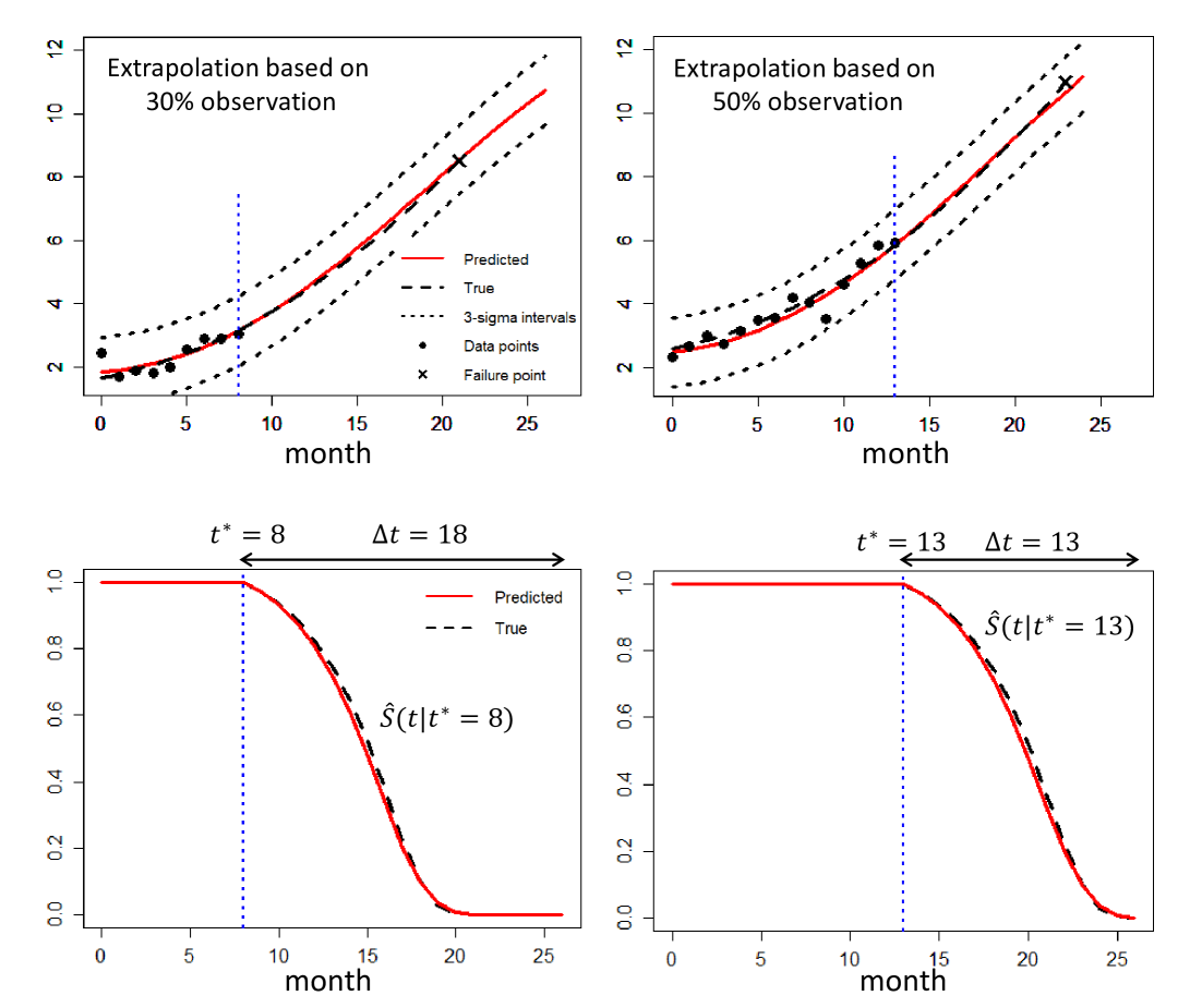
Figure 3: Results of extrapolations and survival probabilities prediction for two testing units. Figures in the first row show results of extrapolations based on different observation percentiles. Figures in the second row show true and predicted survival curves.

4.1 Data setting

For the synthetic data we assume that the underlying true path for unit $i$ has the form $y_{i}(t)=\bm{z}^{T}(t)\bm{b}_{i}+\epsilon_{i}(t)=b_{i0}+b_{i1}t+b_{i2}t^{2}+\epsilon_{i}(t)$, where $\epsilon_{i}(t)\sim\mathcal{N}(0,0.1)$, $\bm{z}^{T}(t)=[1,t,t^{2}]$ and $\bm{b}_{i}=[b_{i0},b_{i1},b_{i2}]^{T}\sim\mathcal{N}(\bm{\mu}_{b},\bm{\Sigma}_{b})$ with $\bm{\mu}_{b}=[2.5,0.1,a]^{T}$ and $\bm{\Sigma}_{b}=\begin{bmatrix}0.2&-4e-4&-8e-5\\ -4e-4&3e-6&3e-7\\ -e-5&3e-7&1e-7\end{bmatrix}$ where $a\sim\mbox{uniform}(0.003,0.03).$ Without loss of generality, we assume that the time unit is month and that signals were obtained regularly at each month up to their failure or censoring time. An example of the signals is shown in the top row of Figure 3. For each unit we specify a time-invariant feature $w_{i}\in\{0,1\}$ generated by a Bernoulli distribution with $p=0.5$. In the Cox model, we use the Weibull baseline hazard rate function $h_{0}(t)=\lambda\rho t^{\rho-1}$ with $\lambda=0.001$ and $\rho=1.05$. We generate the failure time $T_{i}$ for each unit by rejection sampling using its probability density function $h_{i}(t)S_{i}(t)$ . We set $\gamma=0$ and $\beta=0.5$. Also, we randomly select $5\%$ of the units to be right censored. The number of units generated is $N=20$ and the experiment is repeated for $Q=100$ times. Detailed code for data generation is provided in the supplementary materials.

For the real-world case study we use the C-MAPSS dataset provided by the National Aeronautics and Space Administration (NASA). The dataset contains failure time data of aircraft turbofan engines and degradation signals from informative sensors mounted on these engines. Note that in our analysis we standardize all sensor data. We refer readers to Saxena & Goebel (2008) and Liu et al. (2013) for more details about the data. The C-MAPSS data publically available at: https://ti.arc.nasa.gov/tech/dash/groups/pcoe/prognostic-data-repository/.

4.2 Baselines and Evaluations

We focus on predicting the event probability within a future time interval $\Delta t$. We consider $\Delta t=12,15,20$ months in this simulation study. Prediction performance at varying time points $t^{*}$ for the partially observed unit $N$ is then reported. The time instant $t^{*}=\alpha T_{N}$ is defined as the $\alpha$-observation percentile, where $T_{N}$ is the failure time of unit $N$. The values of $\alpha$ are specified as $30\%$, $50\%$. Figure 3 shows some examples of units observed up to different percentiles of their failure time. Further, in our simulation studies, we benchmark our method with three other reference methods for comparison: (1) Logistic Regression (LR) classifier: in the LR, event data is transformed into binary labels $\delta_{i}=1/0$ denoting whether units failed or not within the time interval $[t^{\ast},\Delta t+t^{*}]$. The time-fixed covariate $w_{i}$ and the last observed signal measurement at $t^{\ast}$ are used as the model predictors (2) Support Vector Machine (SVM) classifier: the SVM here is used as a flexible alternative to the LR. We use the radial basis kernel and determine parameters using $2$-fold cross-validation on the training data (3) Parametric Joint Model (LMM-Joint): we implement a state-of-the-art joint modeling algorithm using the linear mixed-effect model. The LMM-joint uses a general polynomial function whose corresponding degree is determined through an Akaike information criteria to model the signal path. Note that this framework estimates parameters from the mixed-effect model and the Cox model separately (Rizopoulos, 2011; Zhou et al., 2014; Mauff et al., 2018). Regarding our MGCP-Cox model we set the number of pseudo-inputs to $M=10$ and the number of latent functions to $K=1$. This setting is a commonly used setting for the MGCP (Álvarez & Lawrence, 2011; Zhao & Sun, 2016). The performance of each method is then assessed by the Receiver Operating Characteristic (ROC) curve, which is a common diagnostic tool for binary classifier. The ROC curve is created by plotting the true positive rate (TPR) against the false positive rate (FPR). Predictive accuracy is then assessed through the area under the curve (AUC). The results from the synthetic data are shown in Figure 4. Due to poor performance of both the LR and SVM on $N=20$, we also checked whether they can produce comparable results to the MGCP-Cox when $N=200$. We denote those models as LR-200 and SVM-200.

For the real data, the true survival probabilities are not available since we do not have information about the underlying parameters used to generate the data. Therefore, to evaluate model performance, we calculate the mean remaining lifetime of the testing unit, which is defined as $\widehat{mrl}(t^{*})=\int_{t^{*}}^{\infty}\hat{S}(u|t^{*},\bm{w}_{N},\bm{f}_{N})du$. This integration can be obtained by the Gauss-Legendre quadrature. The performance is assessed by the absolute error $AE=|{rl}_{j}-\widehat{mrl}_{j}|$ where ${rl}_{j}$ is the true remaining lifetime of the testing unit. We then report the distribution of the errors across all units using the boxplot in Figure 5. Similar to the synthetic data we use 30% and 50% percentiles to assess prediction accuracy. We also note than we cannot obtain $\widehat{mrl}$ estimates from the SVM and LR as they transform event prediction into a time series classification problem. Therefore, only results from LMM-joint and MGCP-Cox are reported in Figure 5.

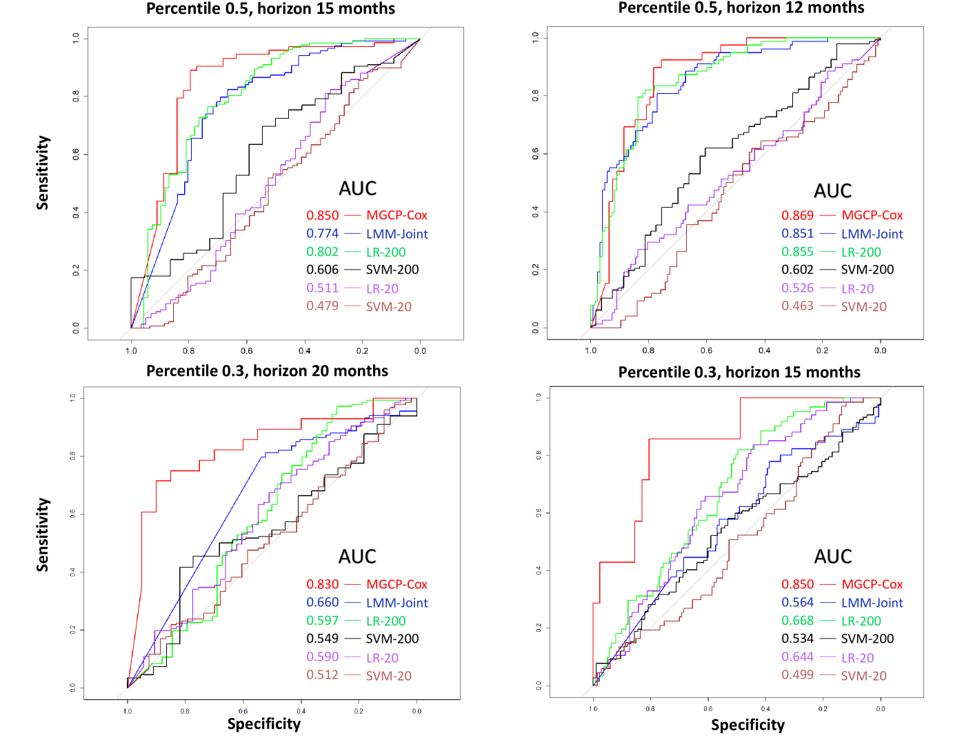
Figure 4: ROC curves from simulation studies under different percentile of observation $\alpha$.

4.3 Results

The illustrative example in Figure 3 demonstrates the behavior of our method. As shown in the figure, our joint model framework can provide accurate predictions of both longitudinal signals and event probabilities. The unique smoothing kernel $G_{i,k}$ for each individual allows flexibility in the prediction, since it enables each training signal to have its own characteristics. This substantiates the strength of the MGCP. Equipped with the shared latent processes, the model can infer the similarities among all units, and predict signal trajectory by borrowing strength from training units.

The results in Figures 4 and 5 indicate that our MGCP-Cox model clearly outperforms the benchmarked models. Based on the figure we can obtain some important insights. First, as expected, prediction errors significantly decrease as the lifetime percentiles increase. Thus, the prediction accuracy from the MGCP-Cox model will become more accurate as $t^{\ast}$ increases and more data are collected from an online monitored unit. Second, the prediction accuracy slightly decreases as we predict over a longer horizon (i.e. prediction is better for the near future). This is intuitively understandable as accuracy might decrease when predicting over a large region where not many training data might be observed. Third, the results show that the MGCP-Cox clearly outperforms LMM-joint. This result highlights the danger of parametric modeling and demonstrates the ability of our non-parametric approach to avoid model misspecifications. Fourth, even when the LR and SVM had a much larger number of units, the MGCP-Cox was still superior. This observation, also true to the LMM-Joint, highlights the strength of joint models. Lastly, one striking feature, shown in Figures 3, 4 and 5, is that even with a small number of observations ($30\%$ observation percentile) from the testing unit we were still able to get accurate predictive results. This crucial in many applications as its allows early prediction of an event occurrence such as a disease or machine failure.

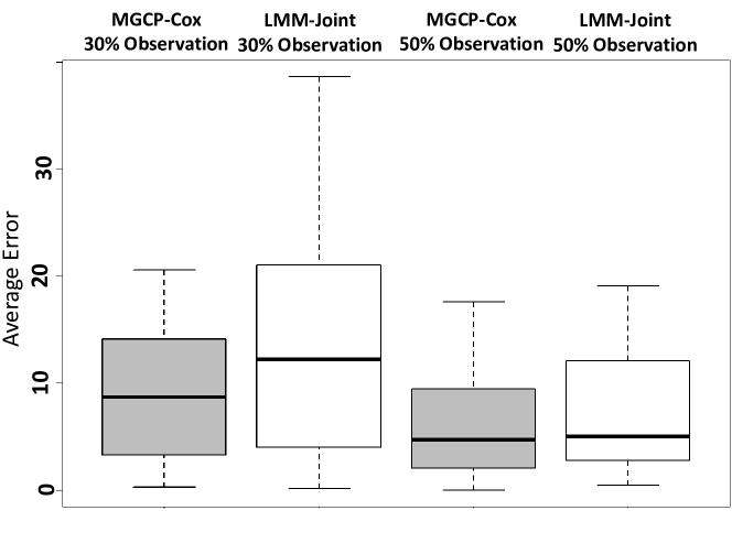
Figure 5: Remaining life prediction accuracy from NASA data.

5 Conclusion

We have presented a flexible and efficient non-parametric joint modeling framework for longitudinal and time-to-event data. A variational inference framework using pseudo-inputs is established to jointly estimate parameters from the MGCP-Cox model. Empirical studies highlight the advantageous features of our model to predict signal trajectories and provide reliable event prediction.

References

- Álvarez & Lawrence (2009) Álvarez, M. and Lawrence, N. D. Sparse convolved gaussian processes for multi-output regression. In Advances in neural information processing systems, pp. 57–64, 2009.
- Álvarez & Lawrence (2011) Álvarez, M. and Lawrence, N. D. Computationally efficient convolved multiple output gaussian processes. Journal of Machine Learning Research, 12(May):1459–1500, 2011.
- Álvarez et al. (2010) Álvarez, M., Luengo, D., Titsias, M., and Lawrence, N. D. Efficient multioutput gaussian processes through variational inducing kernels. In Proceedings of the Thirteenth International Conference on Artificial Intelligence and Statistics, pp. 25–32, 2010.
- Bycott & Taylor (1998) Bycott, P. and Taylor, J. A comparison of smoothing techniques for cd4 data measured with error in a time-dependent cox proportional hazards model. Statistics in medicine, 17(18):2061–2077, 1998.
- Cheng (2018) Cheng, C. Multi-scale gaussian process experts for dynamic evolution prediction of complex systems. Expert Systems with Applications, 99:25–31, 2018.
- Cox (1972) Cox, D. R. Regression models and life-tables. Journal of the Royal Statistical Society: Series B (Methodological), 34(2):187–202, 1972.
- Crowther et al. (2012) Crowther, M. J., Abrams, K. R., and Lambert, P. C. Flexible parametric joint modelling of longitudinal and survival data. Statistics in Medicine, 31(30):4456–4471, 2012.
- Crowther et al. (2013) Crowther, M. J., Abrams, K. R., and Lambert, P. C. Joint modeling of longitudinal and survival data. The Stata Journal, 13(1):165–184, 2013.
- Damianou & Lawrence (2013) Damianou, A. and Lawrence, N. D. Deep gaussian processes. In Artificial Intelligence and Statistics, pp. 207–215, 2013.
- Dempsey et al. (2017) Dempsey, W. H., Moreno, A., Scott, C. K., Dennis, M. L., Gustafson, D. H., Murphy, S. A., and Rehg, J. M. isurvive: An interpretable, event-time prediction model for mhealth. In International Conference on Machine Learning, pp. 970–979, 2017.
- Dürichen et al. (2015) Dürichen, R., Pimentel, M. A., Clifton, L., Schweikard, A., and Clifton, D. A. Multitask gaussian processes for multivariate physiological time-series analysis. IEEE Transactions on Biomedical Engineering, 62(1):314–322, 2015.
- Fernández et al. (2016) Fernández, T., Rivera, N., and Teh, Y. W. Gaussian processes for survival analysis. In Advances in Neural Information Processing Systems, pp. 5021–5029, 2016.
- Gao et al. (2015) Gao, R., Wang, L., Teti, R., Dornfeld, D., Kumara, S., Mori, M., and Helu, M. Cloud-enabled prognosis for manufacturing. CIRP annals, 64(2):749–772, 2015.
- Gasmi et al. (2003) Gasmi, S., Love, C. E., and Kahle, W. A general repair, proportional-hazards, framework to model complex repairable systems. IEEE Transactions on Reliability, 52(1):26–32, 2003.
- Guarnizo & Álvarez (2018) Guarnizo, C. and Álvarez, M. A. Fast kernel approximations for latent force models and convolved multiple-output gaussian processes. arXiv preprint arXiv:1805.07460, 2018.
- He et al. (2015) He, Z., Tu, W., Wang, S., Fu, H., and Yu, Z. Simultaneous variable selection for joint models of longitudinal and survival outcomes. Biometrics, 71(1):178–187, 2015.
- Kalbfleisch & Prentice (2011) Kalbfleisch, J. D. and Prentice, R. L. The statistical analysis of failure time data, volume 360. John Wiley & Sons, 2011.
- Kim & Pavlovic (2018) Kim, M. and Pavlovic, V. Variational inference for gaussian process models for survival analysis. Uncertainty in Artificial Intelligence, 2018.
- Kontar et al. (2018a) Kontar, R., Zhou, S., Sankavaram, C., Du, X., and Zhang, Y. Nonparametric-condition-based remaining useful life prediction incorporating external factors. IEEE Transactions on Reliability, 67(1):41–52, 2018a.
- Kontar et al. (2018b) Kontar, R., Zhou, S., Sankavaram, C., Du, X., and Zhang, Y. Nonparametric modeling and prognosis of condition monitoring signals using multivariate gaussian convolution processes. Technometrics, 60(4):484–496, 2018b.
- Liu et al. (2013) Liu, K., Gebraeel, N. Z., and Shi, J. A data-level fusion model for developing composite health indices for degradation modeling and prognostic analysis. IEEE Transactions on Automation Science and Engineering, 10(3):652–664, 2013.
- Mauff et al. (2018) Mauff, K., Steyerberg, E., Kardys, I., Boersma, E., and Rizopoulos, D. Joint models with multiple longitudinal outcomes and a time-to-event outcome. arXiv preprint arXiv:1808.07719, 2018.
- Moreno-Muñoz et al. (2018) Moreno-Muñoz, P., Artés-Rodríguez, A., and Álvarez, M. A. Heterogeneous multi-output gaussian process prediction. arXiv preprint arXiv:1805.07633, 2018.
- Pham et al. (2012) Pham, H. T., Yang, B., and Nguyen, T. T. Machine performance degradation assessment and remaining useful life prediction using proportional hazard model and support vector machine. Mechanical Systems and Signal Processing, 32:320–330, 2012.
- Proust-Lima et al. (2014) Proust-Lima, C., Séne, M., Taylor, J. M., and Jacqmin-Gadda, H. Joint latent class models for longitudinal and time-to-event data: A review. Statistical methods in medical research, 23(1):74–90, 2014.
- Rizopoulos (2011) Rizopoulos, D. Dynamic predictions and prospective accuracy in joint models for longitudinal and time-to-event data. Biometrics, 67(3):819–829, 2011.
- Rizopoulos (2012) Rizopoulos, D. Joint models for longitudinal and time-to-event data: With applications in R. Chapman and Hall/CRC, 2012.
- Rizopoulos et al. (2017) Rizopoulos, D., Molenberghs, G., and Lesaffre, E. M. Dynamic predictions with time-dependent covariates in survival analysis using joint modeling and landmarking. Biometrical Journal, 59(6):1261–1276, 2017.
- Rosenberg (1995) Rosenberg, P. S. Hazard function estimation using b-splines. Biometrics, pp. 874–887, 1995.
- Ruppert (2002) Ruppert, D. Selecting the number of knots for penalized splines. Journal of computational and graphical statistics, 11(4):735–757, 2002.
- Saxena & Goebel (2008) Saxena, A. and Goebel, K. Turbofan engine degradation simulation data set, 2008. data retrieved from NASA Ames Prognostics Data Repository, https://ti.arc.nasa.gov/tech/dash/groups/pcoe/prognostic-data-repository/.
- Snelson & Ghahramani (2006) Snelson, E. and Ghahramani, Z. Sparse gaussian processes using pseudo-inputs. In Advances in neural information processing systems, pp. 1257–1264, 2006.
- Soleimani et al. (2018) Soleimani, H., Hensman, J., and Saria, S. Scalable joint models for reliable uncertainty-aware event prediction. IEEE transactions on pattern analysis and machine intelligence, 40(8):1948–1963, 2018.
- Titsias & Lawrence (2010) Titsias, M. and Lawrence, N. D. Bayesian gaussian process latent variable model. In Proceedings of the Thirteenth International Conference on Artificial Intelligence and Statistics, pp. 844–851, 2010.
- Tsiatis et al. (1995) Tsiatis, A. A., Degruttola, V., and Wulfsohn, M. S. Modeling the relationship of survival to longitudinal data measured with error. applications to survival and cd4 counts in patients with aids. Journal of the American Statistical Association, 90(429):27–37, 1995.
- Wu et al. (2012) Wu, L., Liu, W., Yi, G. Y., and Huang, Y. Analysis of longitudinal and survival data: joint modeling, inference methods, and issues. Journal of Probability and Statistics, 2012, 2012.
- Wulfsohn & Tsiatis (1997) Wulfsohn, M. S. and Tsiatis, A. A. A joint model for survival and longitudinal data measured with error. Biometrics, pp. 330–339, 1997.
- Yan et al. (2016) Yan, H., Liu, K., Zhang, X., and Shi, J. Multiple sensor data fusion for degradation modeling and prognostics under multiple operational conditions. IEEE Transactions on Reliability, 65(3):1416–1426, 2016.
- Yu et al. (2004) Yu, M., Law, N. J., Taylor, J. M., and Sandler, H. M. Joint longitudinal-survival-cure models and their application to prostate cancer. Statistica Sinica, pp. 835–862, 2004.
- Zhao & Sun (2016) Zhao, J. and Sun, S. Variational dependent multi-output gaussian process dynamical systems. The Journal of Machine Learning Research, 17(1):4134–4169, 2016.
- Zhou et al. (2014) Zhou, Q., Son, J., Zhou, S., Mao, X., and Salman, M. Remaining useful life prediction of individual units subject to hard failure. IIE Transactions, 46(10):1017–1030, 2014.
- Zhu et al. (2012) Zhu, H., Ibrahim, J. G., Chi, Y., and Tang, N. Bayesian influence measures for joint models for longitudinal and survival data. Biometrics, 68(3):954–964, 2012.