High Order Edge Sensors with $\ell^{1}$ Regularization for Enhanced Discontinuous Galerkin Methods

Abstract

This paper investigates the use of $\ell^{1}$ regularization for solving hyperbolic conservation laws based on high order discontinuous Galerkin (DG) approximations. We first use the polynomial annihilation method to construct a high order edge sensor which enables us to flag “troubled” elements. The DG approximation is enhanced in these troubled regions by activating $\ell^{1}$ regularization to promote sparsity in the corresponding jump function of the numerical solution. The resulting $\ell^{1}$ optimization problem is efficiently implemented using the alternating direction method of multipliers. By enacting $\ell^{1}$ regularization only in troubled cells, our method remains accurate and efficient, as no additional regularization or expensive iterative procedures are needed in smooth regions. We present results for the inviscid Burgers’ equation as well as for a nonlinear system of conservation laws using a nodal collocation-type DG method as a solver.

1 Introduction

This work is about a novel shock capturing procedure in spectral element (SE) type of methods for solving time-dependent hyperbolic conservation laws

$$\partial_{t}u+\partial_{x}f(u)=0,$$ (1)

with smooth and discontinuous solutions. Such methods include the spectral difference (SD) [1, 2], discontinuous Galerkin (DG) [3], and flux reconstruction [4] methods. While all these methods provide fairly high orders of accuracy for smooth problems, they often lack desired stability and robustness properties, especially in the presence of (shock) discontinuities.

Many shock capturing techniques have therefore been developed over the last few decades. Such efforts date back more than $60$ years to the pioneering work of von Neumann and Richtmyer, [5] in which they add artificial viscosity terms to (1) in order to construct stable finite difference schemes for the equations of hydrodynamics. Since then, artificial viscosity has been added to a variety of algorithms [6, 7, 8, 9, 10, 11]. However, augmenting (1) with additional (higher) viscosity terms requires care about their design and size. Otherwise, new time stepping constraints for explicit methods can considerably decrease computational efficiency; see, e.g. [8, equation (2.1)]. Other interesting alternatives are based on (modal) filters [12, 13, 10] or applying viscosity to the different spectral scales [14, 15]. Finally, we mention those methods based on order reduction [16], mesh adaptation [17], and weighted essentially nonoscillatory (WENO) concepts [18, 19]. Yet, a number of issues regarding the fundamental convergence properties for these methods still remain unresolved. Moreover, even when the extension to multiple dimensions is straightforward, these schemes may be too computationally expensive for practical usage.

In this work we propose $\ell^{1}$ regularization as a novel tool to capture shocks in SE methods by promoting sparsity in the jump function of the approximate solution. $\ell^{1}$ regularization methods are frequently encountered in signal processing and imaging applications. They are still of limited use in solving partial differential equations numerically, however, and only a few studies, (see, e.g., [20, 21, 22, 23, 24, 25]) have considered sparsity or $\ell^{1}$ regularization of the numerical solution. A brief discussion of these investigations can be found in [24]. We note that while problems with discontinuous initial conditions were studied in [22, 23, 25], problems that form shocks were not. The technique developed in [20] was designed to promote sparsity in the frequency domain, making it less amenable to problems emitting shocks, where the frequency domain is not sparse. Further, with the exception of [24], each of these investigations applied $\ell^{1}$ regularization directly to numerical solution or to its residual, rather than incorporating it directly in the time stepping evolution.

In this investigation we follow the approach in [24], which incorporates $\ell^{1}$ regularization directly into the time dependent solver. Specifically, we promote the sparsity of the jump function that corresponds to the discontinuous solution. The jump function approximation is performed using the (high order) polynomial annihilation (PA) operator [26, 27, 28], which eliminates the unwanted “staircasing” effect, a common degradation of detail of the piecewise smooth solution arising from the classical total variation (TV) regularization. More specifically, the high order PA operator allows the resulting solution to be comprised of piecewise polynomials instead of piecewise constants. We solve the resulting $\ell^{1}$ optimization problem by the alternating direction method of multipliers (ADMM) [29, 30, 31]. A similar application of $\ell_{1}$ regularization was used in [24] to numerically solve hyperbolic conservation laws, though only for the Lax–Wendroff scheme and Chebyshev and Fourier spectral methods. It was concluded in [24] that although the Lax–Wendroff scheme yielded sufficient accuracy for relatively simple problems, its lower order convergence properties made it difficult to resolve more complicated ones. The new technique fared better using Chebyshev polynomials, although their global construction made it difficult to resolve the local structures without oscillations or excessive smoothing.

One possible solution is to use SE methods as the underlying mechanism for solving the hyperbolic conservation law. SE methods have the advantage of being more localized, for instance, and allow element-to-element variations in the optimization problem. In particular for the method we develop here, $\ell^{1}$ regularization is only activated in troubled elements, i.e., in elements where discontinuities are detected. This further enhances efficiency of the method. In the process, a novel discontinuity sensor based on PA operators of increasing orders is proposed, which is able to flag troubled elements. The discontinuity sensor steers the optimization problem and thus locally calibrates the method with respect to the smoothness of the solution. Numerical tests are performed for a nodal collocation-type DG method and the inviscid Burgers’ equation as well as for a nonlinear system. It should be stressed that the proposed procedure also carries over to other classes of methods, with the obvious extension to SE type methods. The extension to other types of methods, such as finite volume methods, is also possible under slight modifications of the procedure. We should also stress that in our new development of the $\ell^{1}$ regularization method for solving PDEs that admit shocks in their solutions that we do not require different methods to be used in smooth and nonsmooth regions. Such methods have been developed in, for instance, [32] and have been shown to be effective. Here we demonstrate that it is possible to avoid such additional complexities.

The rest of this paper is organized as follows: §2 briefly reviews the nodal collocation-type DG method, $\ell^{1}$ regularization, and PA operators which are needed for the development of our method. In §3 we describe the application of $\ell^{1}$ regularization by higher-order edge detectors to SE type methods. Further, a novel discontinuity sensor based on PA operators of increasing orders is proposed. Numerical tests for the inviscid Burgers’ equation, the linear advection equation, and a nonlinear system of conservation laws are presented in §4. The tests demonstrate that we are able to better resolve numerical solutions when $\ell^{1}$ regularization is utilized. We close this work with concluding thoughts in §5.

2 Preliminaries

In this section we briefly review all necessary concepts in order to introduce $\ell^{1}$ regularisation into the framework of discontinuous Galerkin methods in the subsequent section.

2.1 A nodal discontinuous Galerkin method

Let us consider a hyperbolic conservation law

$$\partial_{t}u+\partial_{x}f\left(u\right)=0,\quad x\in\Omega,$$ (2)

with suitable initial and boundary conditions. The domain $\Omega\subset\mathbb{R}$ is decomposed into $I$ disjoint, face-conforming elements $\Omega_{i}$, $\Omega=\bigcup_{i=1}^{I}\Omega_{i}$. All elements are mapped to a reference element, typically $\Omega_{\mathrm{ref}}=[-1,1]$, where all computations are performed.

In this work we consider a nodal collocation-type discontinuous Galerkin (DG) method [3] on the reference element. The solution $u$ as well as the flux function $f$ are approximated by interpolation polynomials of the same degree, giving the advantage of highly efficient operators. We further collocate the flux approximation based on interpolation with the numerical quadrature used for the evaluation of the inner products [33].

The first step is to introduce a nodal polynomial approximation

$$u\left(t,\xi\right)\approx u_{p}\left(t,\xi\right)=\sum_{k=0}^{p}u_{k}\left(t\right)\ell_{k}\left(\xi\right),$$ (3)

where $p$ is the polynomial degree and $\{u_{k}\}_{k=0}^{p}$ are the $p+1$ time dependent nodal degrees of freedom at the element grid nodes $-1\leq\xi_{0}<\dots<\xi_{p}\leq 1$. Common choices are either the Gauss-Legendre or Gauss-Lobatto nodes [34]. We use Gauss-Lobatto points in the latter numerical tests, as they include the boundary points $\xi_{0}=-1,\xi_{p}=1$ and thus render the method more robust [35, 36, 37]. For the procedure of $\ell^{1}$ regularisation proposed in this work the specific choice of grid nodes is not crucial however.

Further, the Lagrange basis functions of degree $p$ are given by

$$\ell_{k}\left(\xi\right)=\prod_{\begin{smallmatrix}i=0\\ i\neq k\end{smallmatrix}}^{p}\frac{\xi-\xi_{i}}{\xi_{k}-\xi_{i}}$$ (4)

and satisfy the cardinal property $\ell_{k}\left(\xi_{i}\right)=\delta_{ki}$. The flux function is approximated in the same way, i.e.

$$f\left(u\right)\approx f_{p}\left(t,\xi\right)=\sum_{k=0}^{p}f_{k}\left(t\right)\ell_{k}\left(\xi\right),$$ (5)

where, collocating the nodes for both approximations, the nodal degrees of freedom $\{f_{k}\}_{k=0}^{p}$ are given by $f_{k}\left(t\right)=f\left(u_{k}\left(t\right)\right)$.

We now obtain the formulation of the nodal DG method by inserting the polynomial approximations (3) and (5) into the conservation law (2), multiplying by a test function $\ell\in\{\ell_{k}\}_{k=0}^{p}$, integrating over the reference element, and applying integration by parts, resulting in

$$\int_{-1}^{1}\dot{u}_{p}\ell_{i}\mathrm{d}\xi+\Bigl{.}\left(f^{\mathrm{num}}\ell_{i}\right)\Bigr{|}_{-1}^{1}-\int_{-1}^{1}f_{p}\ell_{i}^{\prime}\mathrm{d}\xi,\quad i=0,\dots,p.$$ (6)

Here, $f^{\mathrm{num}}$ is a suitably chosen numerical flux, providing a mechanism to couple the solutions across elements [38]. Further, $\dot{u}_{p}$ denotes the time derivative of the approximation while $\ell_{i}^{\prime}$ denotes the spatial derivative of the basis element with respect to $\xi$.

Next, the integrals are approximated by an (interpolatory) quadrature rule using the same nodes,

$$\int_{-1}^{1}g\left(\xi\right)\mathrm{d}\xi\approx\int_{-1}^{1}\sum_{k=0}^{p}g\left(\xi_{k}\right)\ell_{k}\left(\xi\right)\mathrm{d}\xi=\sum_{k=0}^{p}\omega_{k}g\left(\xi_{k}\right).$$ (7)

From this quadrature rule, we introduce a discrete inner product

$$\left\langle{u,\,v}\right\rangle_{\underline{\underline{M}}\,}=\sum_{k=0}^{p}\omega_{k}u\left(\xi_{k}\right)v\left(\xi_{k}\right)=\underline{u}^{T}\underline{\underline{M}}\,\underline{v}$$ (8)

with mass matrix

$$\underline{\underline{M}}\,=\operatorname{diag}\left([\omega_{0},\dots,\omega_{p}]\right)$$ (9)

and vectors of nodal degrees of freedom

$$\underline{u}=[u_{0},\dots,u_{p}]^{T},\quad\underline{v}=[v_{0},\dots,v_{p}]^{T}.$$ (10)

Using the discrete inner product, the spacial approximation (6) becomes

$$\left\langle{\dot{u}_{p},\,\ell_{i}}\right\rangle_{\underline{\underline{M}}\,}=\left\langle{f_{p},\,\ell_{i}^{\prime}}\right\rangle_{\underline{\underline{M}}\,}-\Bigl{.}\left(f^{\mathrm{num}}\ell_{i}\right)\Bigr{|}_{-1}^{1},\quad i=0,\dots,p.$$ (11)

Finally going over to a matrix vector representation and utilising the cardinal property of the Lagrange basis functions, the DG approximation can be compactly rewritten in its weak form as

$$\underline{\underline{M}}\,\dot{\underline{u}}=\underline{\underline{D}}\,^{T}\underline{\underline{M}}\,\underline{f}-\underline{\underline{R}}\,^{T}\underline{\underline{B}}\,\underline{f}^{\mathrm{num}},$$ (12)

where

$$\underline{\underline{D}}\,=\left(\ell_{i}^{\prime}\left(\xi_{k}\right)\right)_{k,i=0}^{p},\quad\underline{\underline{R}}\,=\begin{pmatrix}0&\dots&0&1\\ 1&0&\dots&0\end{pmatrix},\quad\underline{\underline{B}}\,=\begin{pmatrix}-1&0\\ 0&1\end{pmatrix}$$ (13)

are the differentiation matrix, restriction matrix, and boundary matrix, respectively. Let $\underline{f}^{\mathrm{num}}$ denote the vector containing the values of the numerical flux at the element boundaries. Note that applying integration by parts a second time to (6) would result in the strong form

$$\underline{\underline{M}}\,\dot{\underline{u}}=-\underline{\underline{M}}\,\underline{\underline{D}}\,\underline{f}-\underline{\underline{R}}\,^{T}\underline{\underline{B}}\,\left(\underline{f}^{\mathrm{num}}-\underline{\underline{R}}\,\underline{f}\right)$$ (14)

of the DG approximations. Both forms are equivalent when using summation by parts operators, which satisfy ${\underline{\underline{M}}\,\underline{\underline{D}}\,+\underline{\underline{D}}\,^{T}\underline{\underline{M}}\,=\underline{\underline{R}}\,^{T}\underline{\underline{B}}\,\underline{\underline{R}}\,}$. The strong form (14) can further be recovered as a special case of flux reconstruction schemes [39, 40, 41].

2.2 $\ell^{1}$ regularisation

Let $u\left(\xi\right)=u\left(t,\xi\right)$ be the unknown solution on an element $\Omega_{i}$ transformed into the reference element $\Omega_{\mathrm{ref}}$ and $u_{p}\in\mathbb{P}_{p}\left(\Omega_{\mathrm{ref}}\right)$ a spacial polynomial approximation at fixed time $t$. Assume that some measurable features of $u$ have sparse representation. Consequently, the approximation $u_{p}$ is desired to have this sparse representation as well.

Let $H$ be a regularisation functional which measures sparsity. The objective is to then solve the constrained optimisation problem

$$\operatorname*{arg\,min}_{v\in\mathbb{P}_{p}\left(\Omega_{\mathrm{ref}}\right)}H\left(v\right)\quad\text{s.t.}\quad\mathinner{\!\left\lVert v-u_{p}\right\rVert}=0.$$ (15)

The equality constraint, referred to as the data fidelity term, measures how accurately the reconstructed approximation fits the given data with respect to some seminorm $\mathinner{\!\left\lVert\cdot\right\rVert}$. Typically, the continuous $L^{2}$-norm $\mathinner{\!\left\lVert f\right\rVert}_{2}^{2}=\int|f|^{2}$ or some discrete counterpart is used. The regularisation term $H\left(v\right)$ enforces the known sparsity present in the underlying solution $u$ by penalising missing sparsity in the approximation. The regularisation functional $H$ further restricts the approximation space to a desired class of functions, here $\mathbb{P}_{p}\left(\Omega_{\mathrm{ref}}\right)$. Note that any $p$-norm with $p\leq 1$ will enforce sparsity in the approximation. In this work, we choose $H$ to be the $\ell^{1}$-norm of certain transformations of $v$.

It should be stressed that if $\mathinner{\!\left\lVert\cdot\right\rVert}$ is not just a seminorm but a strictly convex norm, for instance induced by an inner product, the equality constraint immediately and uniquely determines the approximation. Thus, instead of (15), typically the related denoising problem

$$\operatorname*{arg\,min}_{v\in\mathbb{P}_{p}\left(\Omega_{\mathrm{ref}}\right)}H\left(v\right)\quad\text{s.t.}\quad\mathinner{\!\left\lVert v-u_{p}\right\rVert}<\sigma$$ (16)

with $\sigma>0$ is solved, which relaxes the equality constraint on the data fidelity term. Equivalently, the denoising problem (16) can also be formulated as the unconstrained (or penalised) problem

$$\operatorname*{arg\,min}_{v\in\mathbb{P}_{p}\left(\Omega_{\mathrm{ref}}\right)}\left(\mathinner{\!\left\lVert v-u_{p}\right\rVert}_{2}^{2}+\lambda H\left(v\right)\right)$$ (17)

by introducing a non-negative regularisation parameter $\lambda\geq 0$. $\lambda$ represents the trade-off between fidelity to the original approximation and sparsity.

The unconstrained problem (17) is often solved with $H\left(v\right)=TV\left(v\right)$, where $TV(v)$ is the total variation of $v$. Following [24] however, in this work we solve (17) with

$$H\left(v\right)=\mathinner{\!\left\lVert L_{m}v\right\rVert}_{1},$$ (18)

where $L_{m}$ is a polynomial annihilation operator introduced in the next subsection. Using higher order polynomial annihilation operators will help to eliminate the staircase effect that occurs when using the TV operator (polynomial annihilation for $m=1$) for $H$, see [42].

2.3 Polynomial annihilation

Polynomial annihilation (PA) operators were originally proposed in [27]. One main advantage in using PA operators of higher orders ($m>1$) for the regularisation functional $H$ is that they allow distinction between jump discontinuities and steep gradients, which is critical in the numerical treatment of nonlinear conservation laws. PA regularisation is also preferable to TV regularisation when the resolution is poor, even when the underlying solution is piecewise constant.

Let $u\left(\xi^{-}\right)$ and $u\left(\xi^{+}\right)$ respectively denote the left and right hand side limits of $u\mathrel{\mathop{\ordinarycolon}}\Omega_{\mathrm{ref}}=[a,b]\to\mathbb{R}$ at $\xi$. We define the jump function of $u$ as

$$[u]\left(\xi\right)=u\left(\xi^{+}\right)-u\left(\xi^{-}\right)$$ (19)

and note that $[u]\left(\xi\right)=0$ at every $\xi\in\Omega_{\mathrm{ref}}$ where $u$ has no jump. We thus say that the jump function $[u]$ has a sparse representation. The polynomial annihilation operator of order $m$,

$$L_{m}[u]\left(\xi\right)=\frac{1}{q_{m}\left(\xi\right)}\sum_{x_{j}\in S_{\xi}}c_{j}\left(\xi\right)u\left(x_{j}\right),$$ (20)

is designed in order to approximate the jump function $\left[u\right]$. Here

$$S_{\xi}=\{x_{0}\left(\xi\right),\dots,x_{m}\left(\xi\right)\}\subset\Omega_{\mathrm{ref}}$$ (21)

is a set of $m+1$ local grid points around $\xi$, the annihilation coefficients $c_{j}\mathrel{\mathop{\ordinarycolon}}\Omega_{\mathrm{ref}}\to\mathbb{R}$ are given by

$$\sum_{x_{j}\in S_{\xi}}c_{j}\left(\xi\right)p_{l}\left(x_{j}\right)=p_{l}^{\left(m\right)}\left(\xi\right),\quad j=0,\dots,m,$$ (22)

and $\{p_{l}\}_{l=0}^{m}$ is a basis of $\mathbb{P}_{m}\left(\Omega_{\mathrm{ref}}\right)$. An explicit formula for the annihilation coefficients utilising Newton’s divided differences is given by ([27]):

$$c_{j}\left(\xi\right)=\frac{m!}{\omega_{j}\left(S_{\xi}\right)}\quad\text{with}\quad\omega_{j}\left(S_{\xi}\right)=\prod_{\begin{smallmatrix}x_{i}\in S_{\xi}\\ i\neq j\end{smallmatrix}}\left(x_{j}-x_{i}\right)$$ (23)

for $j=0,\dots,m$. Finally, the normalisation factor $q_{m}$, calculated as

$$q_{m}\left(\xi\right)=\sum_{x_{j}\in S_{\xi}^{+}}c_{j}\left(\xi\right),$$ (24)

ensures convergence to the right jump strength at every discontinuity. Here $S_{\xi}^{+}$ denotes the set $\{x_{j}\in S_{\xi}\ |\ x_{j}\geq\xi\}$ of all local grid points to the right of $\xi$.

In this work, the PA operator is applied to the reference element $\Omega_{\mathrm{ref}}=[-1,1]$ of the underlying nodal DG method using $p+1$ collocation points $\{\xi_{k}\}_{k=0}^{p}$, typically Gauss-Lobatto points including the boundaries. We can thus construct polynomial annihilation operators up to order $p$ by allowing the sets of local grid points $S_{\xi}$ to be certain subsets of the $p+1$ collocation points.

In [27] it was shown that

$$L_{m}[u]\left(\xi\right)=\left\{\begin{array}[]{ccl}[u]\left(x\right)+\mathcal{O}\left(h\left(\xi\right)\right)&,&\text{if }x_{j-1}\leq\xi,x\leq x_{j},\\ \mathcal{O}\left(h^{\min\left(m,k\right)}\left(\xi\right)\right)&,&\text{if }u\in C^{k}\left(I_{\xi}\right),\end{array}\right.$$ (25)

where $h\left(\xi\right)=\max\{|x_{i}-x_{i-1}\ |\ x_{i-1},x_{i}\in S_{\xi}\}$ and $I_{\xi}$ is the smallest closed interval such that $S_{\xi}\subset I_{\xi}$. Note that $h(\xi)$ depends on the density of set of local grid points around $\xi$. Thus, $L_{m}$ provides $m$th order convergence in regions where $u\in C^{m}$, and yields a first order approximation to the jump. It should be stressed that oscillations develop around points of discontinuity as $m$ increases. The impact of the oscillation could be reduced by post-processing methods, such as the minmod limiter, as was done in [27]. However, as long as there is sufficient resolution between two shock locations, such oscillations do not directly impact our method. This is because we use the PA operator not to detect the precise location of jump discontinuities, but rather to enforce sparsity.

Figures 1(b) and 1(c) demonstrate the PA operator for the discontinuous function illustrated in Figure 1(a), while Figures 1(e) and 1(f) do so for the continuous but not differentiable function shown in Figure 1(g), and Figures 1(h) and 1(i) illustrate the PA operator for the smooth function in Figure 1(g).

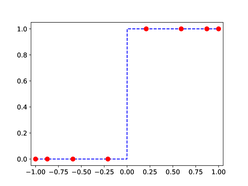
(a) $f_{1}(\xi)$

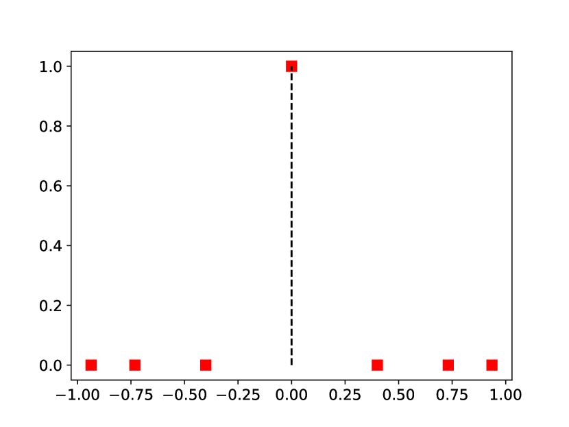
(b) $f_{1}(\xi)$, PA for $m=1$

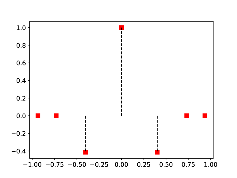
(c) $f_{1}(\xi)$, PA for $m=3$

(d) $f_{2}(\xi)$

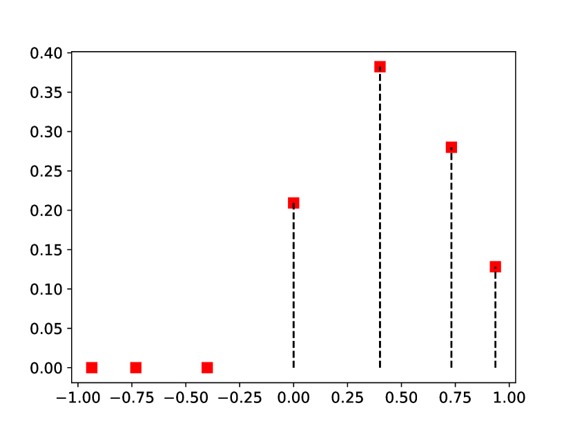
(e) $f_{2}(\xi)$, PA for $m=1$

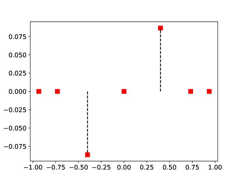
(f) $f_{2}(\xi)$, PA for $m=3$

(g) $f_{3}(\xi)$

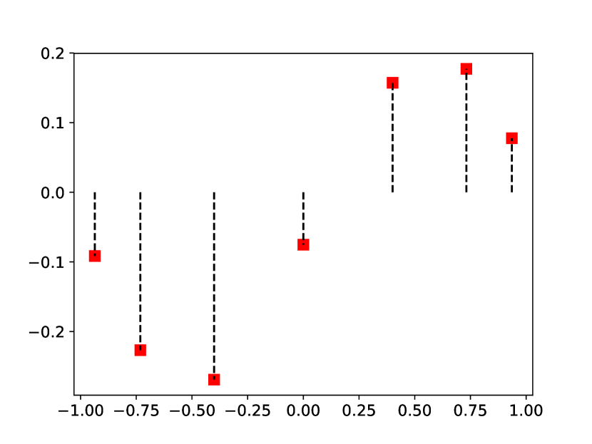
(h) $f_{3}(\xi)$, PA for $m=1$

(i) $f_{3}(\xi)$, PA for $m=3$

Figure 1: Three different functions $f$ at $8$ Gauss-Lobatto points. The PA operator is evaluated at their mid points.

        

For each function we used eight Gauss-Lobatto points to compute the PA operators for $m=1,3$ at the mid points $\xi_{j+1/2}=\left(\xi_{j-1}+\xi_{j}\right)/2$. As illustrated in Figure 1(b) and 1(c), the jump function approximation becomes oscillatory as $m$ is increased from $1$ to $3$, especially in the region of the discontinuity. The maximal absolute value of the PA operator is also not decreasing in this case. On the other hand, for the continuous and smooth functions displayed in Figures 1(d) and 1(g), the maximal absolute value decreases significantly when going from $m=1$ to $m=3$. This is consistent with the results in (25), and will be used to construct the discontinuity sensor in §3.3. For a discussion on the convergence of the PA operator see [27].

Remark 1.

In this work, we only consider one dimensional conservation laws. It should be stressed, however, that polynomial annihilation can be extended to multivariate irregular data in any domain. It was demonstrated in [27] that polynomial annihilation is numerically cost efficient and entirely independent of any specific shape or complexity of boundaries. In particular, in [43] and [44] the method was applied to high dimensional functions that arise when solving stochastic partial differential equations, which reside in a high dimensional space which includes the original space and time domains as well as additional random dimensions.

3 Application of $\ell_{1}$ regularization

In this section, we describe how the proposed $\ell^{1}$ regularization using PA operators, i.e., $H\left(v\right)=\mathinner{\!\left\lVert L_{m}v\right\rVert}_{1}$ in (17), can be incorporated into a DG method. While this kind of regularization functional was already investigated in [24], this work is the first to extend these ideas to an SE method and thus to allow element-to-element variations in the optimization problem. It should be stressed that the subsequent procedure relies on a piecewise polynomial approximation in space. Yet, by appropriate modifications of the procedure, it is also possible to apply $\ell^{1}$ regularization (with PA) to any other method.

3.1 Procedure

One of the main challenges in solving nonlinear conservation laws (2) is balancing high resolution properties and the amount of viscosity introduced to maintain stability, especially near shocks [5, 7, 11]. Applying the techniques presented in §2.2 and §2.3, we are now able to adapt the nodal DG method described in §2.1 to include $\ell^{1}$ regularization.

Our procedure consists of replacing the usual polynomial approximation $u_{p}$ by a sparse reconstruction

$$u_{p}^{\mathrm{spar}}=\operatorname*{arg\,min}_{v\in\mathbb{P}_{p}\left(\Omega_{\mathrm{ref}}\right)}\left(\frac{1}{2}\mathinner{\!\left\lVert v-u_{p}\right\rVert}_{2}^{2}+\lambda\mathinner{\!\left\lVert L_{m}v\right\rVert}_{1}\right)$$ (26)

with regularization parameter $\lambda$ in troubled elements after every (or every $k$th) time step by an explicit time integrator.

For the ADMM described in §3.5, it is advantageous to rewrite (26) in the usual form of an $\ell^{1}$ regularized problem as

$$u_{p}^{\mathrm{spar}}=\operatorname*{arg\,min}_{v\in\mathbb{P}_{p}\left(\Omega_{\mathrm{ref}}\right)}\left(\mathinner{\!\left\lVert L_{m}v\right\rVert}_{1}+\frac{\mu}{2}\mathinner{\!\left\lVert v-u_{p}\right\rVert}_{2}^{2}\right),$$ (27)

where $\mu=\frac{2}{\lambda}$ is referred to as the data fidelity parameter. Note that (26) and (27) are equivalent. In the later numerical tests, the data fidelity parameter $\mu$ and the regularization parameter $\lambda$ will be steered by a discontinuity sensor proposed in §3.3.

Remark 2.

One of the main drawbacks in using $\ell^{1}$ regularization for solving numerical partial differential equations, as well as for image restoration or sparse signal recovery, is in choosing the regularization parameter $\lambda$ (or $\mu$). Ideally, one would want to balance the terms in (26) or (27), but this is difficult to do without knowing their comparative size. Indeed, the $\ell^{1}$ regularization term $\mathinner{\!\left\lVert L_{m}v\right\rVert}_{1}$ heavily depends on the magnitudes of nonzero values in the sparsity domain, in this case the jumps. Larger jumps are penalized significantly more in the $\ell^{1}$ norm than smaller values.

Iterative spacially varying weighted $\ell^{1}$ regularization techniques (see, e.g., [45, 46]) are designed to help reduce the size of the norm, since the remaining values should be close to zero in magnitude. Specifically, the jump discontinuities which are meant to be in the solution can “pass through” the minimization. In this way, with some underlying assumptions made on the accuracy of the fidelity term, one could argue that both terms are close to zero. Consequently, the choice of $\lambda$ (or $\mu$) should not have as much impact on the results, leading to greater robustness overall. For the numerical experiments in this investigation, we simply chose regularization parameters that worked well. We did not attempt to optimize our results and leave parameter selection to future work.

3.2 Selection of the regularization parameter $\lambda$

The $\ell^{1}$ regularization should only be activated in troubled elements. In particular, we do not want to unnecessarily degrade the accuracy in the smooth regions of the solution. We thus propose to adapt the regularization parameter $\lambda$ in (26) to appropriately capture different discontinuities and regions of smoothness. As a result, the optimization problem will be able to calibrate the resulting sparse reconstruction to the smoothness of the solution. More specifically, to avoid unnecessary regularization, we choose $\lambda=0$ in elements corresponding to smooth regions. Note that this also renders the proposed method more efficient.

On the other hand, when a discontinuity is detected in an element, $\ell^{1}$ regularization will be fully activated by choosing $\lambda=\lambda_{\text{max}}$ in (26), which corresponds to the amount of regularization necessary to reconstruct sharp shock profiles. While no effort was made to optimize or even adapt this parameter, we found that using $\lambda_{\text{max}}=4\cdot 10^{2}$ in all of our numerical experiments yielded good results. A heuristic explanation for choosing $\lambda_{\text{max}}$ in this way stems from the goal of balancing the size of $\mathinner{\!\left\lVert L_{m}v\right\rVert}_{1}$ with the expected size of the fidelity term, which in this case means to be consistent with the order of accuracy of the underlying numerical PDE solver. As mentioned previously, choosing an appropriate $\lambda$ will be the subject of future work.

Between these extreme cases, i.e., $\lambda=0$ and $\lambda=\lambda_{\text{max}}$, we allow the regularization parameter to linearly vary and choose $\lambda$ as a function of the discontinuity sensor proposed in §3.3. As a consequence, we obtain more accurate sparse reconstructions while still maintaining stability in regions around discontinuities.

3.3 Discontinuity sensor

We now describe the discontinuity sensor which is used to activate the $\ell^{1}$ regularization and to steer the regularization parameter $\lambda$ in (26). The sensor is based on comparing PA operators of increasing orders. To the best of our knowledge this is the first time the PA operator is utilized for shock (discontinuity) detection in a PDE solver.

At least for smooth solutions, discontinuous Galerkin methods are capable of spectral orders of accuracy. $\ell^{1}$ regularization as well as any other shock capturing procedure [5, 7, 13, 10, 11] should thus be just applied in (and near) elements where discontinuities are present. We refer to those elements as troubled elements.

Many shock and discontinuity sensors have been proposed over the last $20$ years for the selective application of shock capturing methods. Some of them use information about the $L^{2}$-norm of the residual of the variational form [48, 49], the primary orientation of the discontinuity [50], the magnitude of the facial interelement jumps [51, 52], or entropy pairs [53] to detect troubled elements. Others are not just able to detect troubled elements, but even the location of discontinuities in the corresponding element, such as the concentration method in [54, 55, 56, 57, 58, 32, 59]. The PA operator is also capable of detecting the location of a discontinuity [27, 60, 43] up to the resolution size, as in (25), using nonlinear postprocessing techniques. It should be stressed, however, that in this work we do not fully make use of this feature.

In what follows we present a novel discontinuity sensor based on the PA operator. Let the sensor value of order $m$ be

$$S_{m}=\max_{0\leq k\leq p-1}\left|L_{m}[u_{p}]\left(\xi_{k+\frac{1}{2}}\right)\right|,$$ (28)

i.e., the greatest absolute value of the PA operator at the midpoints

$$\xi_{k+\frac{1}{2}}=\frac{\xi_{k}+\xi_{k+1}}{2},\quad\text{for }k=0,\dots,p-1,$$ (29)

of the collocation points. Since $L_{m}$ provides convergence to $0$ of order $m$ in elements where $u$ has $m$ continuous derivatives, we expect $S_{3}<S_{1}$ to hold for an at least continuous function. Thus, $\ell^{1}$ regularization should just be fully activated if

$$S(u)\mathrel{\mathop{\ordinarycolon}}=\frac{S_{3}}{S_{1}}\geq 1,$$ (30)

i.e., if the sensor value does not decrease as $m$ increases from $1$ to $3$. Sensor values of order $1$ and $3$ (rather than $2$) are chosen since having symmetry of the grid points in $S_{\xi}$ surrounding the point $\xi$ yields a simpler form for implementation [27]. Various modifications of the PA sensor (30) are possible and will be the topic of future research. In the following, the resulting PA sensor is demonstrated for the function displayed in Figure 2 on the interval $[0,10]$. We decompose the interval into $I=5$ elements and apply the PA operator and resulting PA sensor separately on each element.

Figure 2: Test function with various different discontinuities as well as continuous but not differentiable points.

Table 1 lists the sensor values of order $m=1$ and $m=3$ on each element in Figure 2. The last row further shows if the PA sensor (30) reacts. As can be seen in Table 1, the discontinuity sensor exactly identifies the troubled elements, simply by comparing the sensor values of order $m=1$ and $m=3$.

Element	$\Omega_{1}=\left(0,2\right)$	$\Omega_{2}=\left(2,4\right)$	$\Omega_{3}=\left(4,6\right)$	$\Omega_{4}=\left(6,8\right)$	$\Omega_{5}=\left(8,10\right)$
$S_{1}$	1.58	1.07	1.07	2.79	0.38
$S_{3}$	1.99	0.60	1.38	3.00	0.17
Discontinuity	yes	no	yes	yes	no

Table 1: Shock sensor for function displayed in Figure 2.

Even though we use this sensor only to detect troubled elements, in principle, this new sensor can also be used to more precisely determine the location and strength of the discontinuities. Such information can be used for refined domain decomposition [43]. Finally, we decide for the regularization parameter $\lambda$ to linearly vary between $\lambda=0$ and $\lambda=\lambda_{\text{max}}$ and thus utilize the parameter function

$$\lambda(S)=\left\{\begin{array}[]{ll}0&\text{if }S\leq\kappa,\\ \lambda_{\text{max}}(S-\kappa)/(1-\kappa)&\text{if }\kappa<S<1,\\ \lambda_{\text{max}}&\text{if }1\leq S,\\ \end{array}\right.$$ (31)

where $\kappa\in[0,1)$ is a problem dependent ramp parameter. Observe that using $\lambda(S)$ is comparable to employing the weighted $\ell_{1}$ regularization as discussed in Remark 2.

For the later numerical tests we also considered other parameter functions, some as discussed in [61]. Yet the best results were obtained with (31). The same holds for other discontinuity sensors, such as the modal-decay based sensor of Persson and Peraire [7, 61] and its refinements [51, 8] as well as the KXRCF sensor [62, 47] of Krivodonova et al., which is built up on a strong superconvergence phenomenon of the DG method at outflow boundaries. For brevity, those results are omitted here.

Remark 3.

We note that the PA sensor might produce false positive or false negative misidentifications in certain cases. A false negative misidentification might arise from a discontinuity where the solution is detected to be smooth. This is encountered by the ramp parameter $\kappa$, which is observed to work robustly for $\kappa=0.8$ or $\kappa=0.9$ in all later numerical tests. A false positive misidentification might arise from a smooth solution which is detected to be nonsmooth (possibly discontinuous). In this case smooth parts of the solution with steep gradients will result in significantly greater values of $L_{m}u$ than parts of the solution with less steep gradients. As a result, the standard $\ell^{1}$ regularization would heavily penalize these features of the solution, yielding inappropriate smearing of steep gradients in smooth regions. By making $\lambda=\lambda(S)$ dependent on the sensor value, this problem can be somewhat alleviated. Using a weighted $\ell^{1}$ regularization, as suggested in Remark 2, should also reduce the unwanted smearing effect. Failure to detect a discontinuity would, after a number of time steps, yield instability. However it is unlikely that this would occur as the growing oscillations would more likely be identified as shock discontinuities.

3.4 Efficient implementation of the PA operator

While the PA operator was defined on the interior of the reference element $\Omega_{\mathrm{ref}}=[-1,1]$ in §2.3, the shock sensor proposed in §3.3 only relies on the values of the PA operator at the $p$ midpoints $\{\xi_{k+\frac{1}{2}}\}_{k=0}^{p-1}$ of the collocation points $\{\xi_{k}\}_{k=0}^{p}$. The same holds for the $\ell^{1}$ regularization term $H\left(v\right)=\mathinner{\!\left\lVert L_{m}v\right\rVert}_{1}$. The $\ell^{1}$-norm of the PA transformation is thus given by

$$\mathinner{\!\left\lVert L_{m}v\right\rVert}_{1}=\mathinner{\!\left\lVert\underline{\underline{L_{m}}}\,\underline{v}\right\rVert}_{1}=\sum_{k=0}^{p-1}\left|L_{m}[v]\left(\xi_{k+1/2}\right)\right|,$$ (32)

where the vector $\underline{v}$ once more consists of nodal degrees of freedom. We now aim to provide an efficient implementation of the PA operator $L_{m}$ in form of a matrix representation $\underline{\underline{L_{m}}}\,$, which maps the nodal values $\underline{v}$ to the values of the PA operator at the midpoints. Revisiting (20), this matrix representation is given by

$$\underline{\underline{L_{m}}}\,=\underline{\underline{Q}}\,^{-1}\underline{\underline{C}}\,\in\mathbb{R}^{p\times(p+1)}$$ (33)

with

$$\underline{\underline{Q}}\, =\operatorname{diag}\left(\left[q_{m}\left(\xi_{1/2}\right),\dots,q_{m}\left(\xi_{p-1/2}\right)\right]\right),$$ (34)

$$q_{m}\left(\xi_{k+1/2}\right) =\sum_{x_{j}\in S_{\xi_{k+1/2}}^{+}}c_{j}\left(\xi_{k+1/2}\right)$$ (35)

and

$$\underline{\underline{C}}\,=\left(c_{j}\left(\xi_{k+1/2}\right)\right)_{k,j=0}^{p-1,p},$$ (36)

where

$$c_{j}\left(\xi_{k+1/2}\right) =\left\{\begin{array}[]{ll}\frac{m!}{\omega_{j}\left(S_{\xi_{k+1/2}}\right)}&\text{if }x_{j}\in S_{\xi_{k+1/2}},\\ 0&\text{else},\end{array}\right.$$ (39)

$$\omega_{j}\left(S_{\xi_{k+1/2}}\right) =\prod_{\begin{smallmatrix}x_{i}\in S_{\xi_{k+1/2}}\\ i\neq j\end{smallmatrix}}\left(x_{j}-x_{i}\right).$$ (40)

Utilizing all prior matrix vector representations, we can now give the discretization of the $\ell^{1}$ regularized optimization problem (27) by

$$\underline{u}^{\mathrm{spar}}=\operatorname*{arg\,min}_{\underline{v}\in\mathbb{R}^{p+1}}\left(\mathinner{\!\left\lVert\underline{\underline{L_{m}}}\,\underline{v}\right\rVert}_{1}+\frac{\mu}{2}\mathinner{\!\left\lVert\underline{v}-\underline{u}\right\rVert}_{\underline{\underline{M}}\,}^{2}\right).$$ (41)

Thus, we are able to solve the optimization problem directly for the nodal degrees of freedom of the sparse reconstruction $u_{p}^{\mathrm{spar}}$. Alternatively, the fidelity term $\mathinner{\!\left\lVert v-u_{p}\right\rVert}$ can also be approximated as

$$\mathinner{\!\left\lVert\underline{v}-\underline{u}\right\rVert}^{2}_{2}=\sum_{k=0}^{p}\left|v(\xi_{k})-u(\xi_{k})\right|^{2},$$ (42)

i.e., by the Euclidean norm, yielding

$$\underline{u}^{\mathrm{spar}}=\operatorname*{arg\,min}_{\underline{v}\in\mathbb{R}^{p+1}}\left(\mathinner{\!\left\lVert\underline{\underline{L_{m}}}\,\underline{v}\right\rVert}_{1}+\frac{\mu}{2}\mathinner{\!\left\lVert\underline{v}-\underline{u}\right\rVert}_{2}^{2}\right),$$ (43)

instead of (41). Future works will investigate the influence of the choice of the discrete norm on the performance of the $\ell^{1}$ regularization. Here we decided to use the Euclidean norm and thus the minimization problem (43), making the computations in §3.5 more intelligible.

3.5 The alternating direction method of multipliers

Many techniques have been recently proposed to solve optimization problems in the form of (41). Following [24], we use the ADMM [29, 30, 31] in our implementation. The ADMM has its roots in [63] and details of its convergence properties can be found in [64, 65, 66]. In the context of $\ell^{1}$ regularization, ADMM is commonly implemented using the split Bregman method [67], which is known to be an efficient solver for a broad class of optimization problems. To implement the ADMM, it is first necessary to eliminate all nonlinear terms within the $\ell^{1}$-norm. We thus introduce a slack variable

$$\underline{g}=\underline{\underline{L_{m}}}\,\underline{v}\in\mathbb{R}^{p}$$ (44)

and formulate (41) equivalently as

$$\operatorname*{arg\,min}_{\underline{v}\in\mathbb{R}^{p+1},\underline{g}\in\mathbb{R}^{p}}\left(\mathinner{\!\left\lVert\underline{g}\right\rVert}_{1}+\frac{\mu}{2}\mathinner{\!\left\lVert\underline{v}-\underline{u}\right\rVert}_{2}^{2}\quad\text{s.t.}\quad\underline{\underline{L_{m}}}\,\underline{v}=\underline{g}\right).$$ (45)

To solve (45), we further introduce Lagrangian multipliers $\underline{\sigma}\in\mathbb{R}^{p},\underline{\delta}\in\mathbb{R}^{p+1}$ and solve the unconstrained minimization problem given by

$$\operatorname*{arg\,min}_{\underline{v}\in\mathbb{R}^{p+1},\underline{g}\in\mathbb{R}^{p}}J_{\underline{\sigma},\underline{\delta}}\left(\underline{v},\underline{g}\right)$$ (46)

with objective function

$$J_{\underline{\sigma},\underline{\delta}}\left(\underline{v},\underline{g}\right)=\mathinner{\!\left\lVert\underline{g}\right\rVert}_{1}+\frac{\mu}{2}\mathinner{\!\left\lVert\underline{v}-\underline{u}\right\rVert}_{2}^{2}+\frac{\beta}{2}\mathinner{\!\left\lVert\underline{\underline{L_{m}}}\,\underline{v}-\underline{g}\right\rVert}_{2}^{2}-\left\langle{\underline{\underline{L_{m}}}\,\underline{v}-\underline{g},\,\underline{\sigma}}\right\rangle_{2}-\left\langle{\underline{v}-\underline{u},\,\underline{\delta}}\right\rangle_{2}.$$ (47)

Here, $\beta>0$ is an additional positive regularization parameter and recall that the data fidelity parameter $\mu$ is given by $\mu=\frac{2}{\lambda}$ for $\lambda>0$; see (26) and (27). Note that if the Lagragian multipliers $\underline{\sigma},\underline{\delta}$ are updated a sufficient number of times, the solution of the unconstrained problem (46) will converge to the solution of the constrained problem (45). In the ADMM, the solution is approximated by alternating between minimizations of $\underline{v}$ and $\underline{g}$. A crucial advantage of this method is that, given the current value of $\underline{v}$ as well as the Lagrangian multipliers, the optimal value of g can be exactly determined by the shrinkage-like formula [67]

$$\left(\underline{g}_{k+1}\right)_{i}=shrink\left(\left(\underline{\underline{L_{m}}}\,\underline{v}\right)_{i}-\frac{1}{\beta}\left(\underline{\sigma}_{k}\right)_{i},\frac{1}{\beta}\right),$$ (48)

where

$$shrink\left(x,\gamma\right)=\frac{x}{|x|}\cdot\max\left(|x|-\gamma,0\right).$$ (49)

Given the current value $\underline{g}_{k+1}$, on the other hand, the optimal value of $\underline{v}$ is computed by the gradient descent method as

$$\underline{v}_{k+1}=\underline{v}_{k}-\alpha\nabla_{\underline{v}}J_{\underline{\sigma},\underline{\delta}}\left(\underline{v},\underline{g}_{k+1}\right),$$ (50)

where

$$\nabla_{\underline{v}}J_{\underline{\sigma},\underline{\delta}}\left(\underline{v},\underline{g}_{k+1}\right)=\mu\left(\underline{v}-\underline{u}\right)+\beta\left(\underline{\underline{L_{m}}}\,\right)^{T}\left(\underline{\underline{L_{m}}}\,\underline{v}-\underline{g}_{k+1}\right)-\left(\underline{\underline{L_{m}}}\,\right)^{T}\underline{\sigma}_{k}-\underline{\delta}_{k},$$ (51)

and the step size $\alpha>0$ is chosen to provide a sufficient descent in direction of the gradient. Finally, the Lagrangian multipliers are updated after each iteration by

$$\underline{\sigma}_{k+1} =\underline{\sigma}_{k}-\beta\left(\underline{\underline{L_{m}}}\,\underline{v}_{k+1}-\underline{g}_{k+1}\right),$$ (52)

$$\underline{\delta}_{k+1} =\underline{\delta}_{k}-\mu\left(\underline{v}_{k+1}-\underline{u}\right).$$

Algorithm 1 is borrowed from [31, 24] and compactly describes the above ADMM.

Algorithm 1 ADMM

1:Determine parameters $\mu,\beta$, and $tol$

2:Initialize $\underline{v}_{0},\underline{g}_{0},\underline{\sigma}_{0}$, and $\underline{\delta}_{0}$

3:for $k=0$ to $K$ do

4:     while $\mathinner{\!\left\lVert\underline{v}_{k+1}-\underline{v}_{k}\right\rVert}>tol$ do

5:         Minimize $J$ for $\underline{g}$ according to (48)

6:         Minimize $J$ for $\underline{v}$ according to (50)      

7:     Update the Lagrangian multipliers according to (52)

Figure 3 demonstrates the effect of $\ell^{1}$ regularization to a polynomial approximation with degree $p=13$ of a discontinuous sawtooth function $u(x)=\operatorname{sign}(x)-x$ on $[-1,1]$.

(a) $u_{p}$

(b) $L_{3}[u_{p}]$

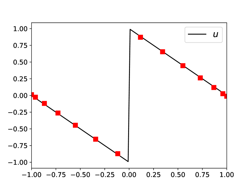
(c) $u_{p}^{spar}$

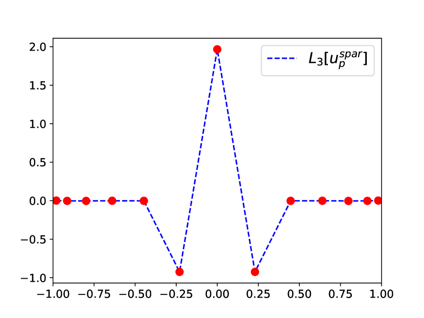
(d) $L_{3}[u_{p}^{spar}]$

Figure 3: Demonstration of $\ell^{1}$ regularization for the polynomial approximation (polluted by the Gibbs phenomenon) of a discontinuous function $u$.

Due to the Gibbs phenomenon, the original polynomial approximation $u_{p}$ in Figure 3(a) shows spurious oscillations [68]. As a consequence, the approximation of the corresponding jump function by the PA operator for $m=3$ in Figure 3(b) also shows undesired oscillations away from the detected discontinuity at $x=0$. Note that the neighboring undershoots around $x=0$ are inherent in the PA operator for $m=3$. Yet, the oscillations left and right from these undershoots stem from the Gibbs phenomenon and thus are parasitical. Applying $\ell^{1}$ regularization to enhance sparsity of the PA transform, however, is able to correct these spurious oscillations, resulting in a sparse representation of the PA transformation in Figure 3(d). The corresponding nodal values, illustrated in Figure 3(c), now approximate the nodal values of the true solution accurately.

For the numerical test in Figure 3, we have chosen the parameters $K=400$, $\mu=0.005$ ($\lambda=4\cdot 10^{2}$), $\beta=20$, $\alpha=0.0001$, and $tol=0.001$. The Lagrangian multipliers have been initialized with $\underline{\sigma}_{0}=\underline{0}$ and $\underline{\delta}_{0}=\underline{0}$.

3.6 Preservation of mass conservation

An essential property of standard (DG) finite element methods for hyperbolic conservation laws is that they are conservative, i.e., that

$$\int_{\Omega}u(t^{n+1},x)\mathrm{d}x=\int_{\Omega}u(t^{n},x)\mathrm{d}x+f\big{|}_{\partial\Omega}$$ (53)

holds [69, 3, 35]. Any reasonable shock capturing procedure for hyperbolic conservation laws should preserve this property as well. In particular, in a troubled element $\Omega_{i}$ in which $\ell^{1}$ regularization is applied,

$$\int_{\Omega_{i}}u_{p}^{\mathrm{spar}}(x)\mathrm{d}x=\int_{\Omega_{i}}u_{p}(x)\mathrm{d}x$$ (54)

should hold in order for $\ell^{1}$ regularization to preserve mass conservation of the underlying (DG) method. Unfortunately, (54) is violated when $\ell^{1}$ regularization is applied too naively. This is demonstrated in Figure 4 for a simple discontinuous example $u(x)=\operatorname{sign}(x-0.5)+1$ on $\Omega_{\mathrm{ref}}=[-1,1]$ with mass $\int_{\Omega_{\mathrm{ref}}}u\mathrm{d}x=1$.

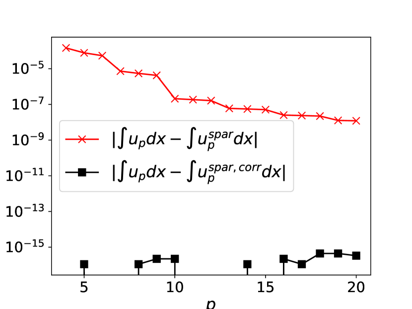
Figure 4: Absolute difference between the mass of $u_{p}$ and $u_{p}^{\mathrm{spar}}$ (red crosses) and between the mass of $u_{p}$ and $u_{p}^{\mathrm{spar,corr}}$ (black squares) for $u(x)=\operatorname{sign}(x-0.5)+1$ on $\Omega_{\mathrm{ref}}=[-1,1]$ and increasing polynomial degree $p=4,\dots,20$. In the cases where no (black) squares are visible the difference was below machine precision.

The (red) crosses illustrate the absolute difference between the mass of the polynomial interpolation $u_{p}$ and its sparse reconstruction $u_{p}^{\mathrm{spar}}$, i.e.

$$\left|\int_{\Omega_{\mathrm{ref}}}u_{p}(x)\mathrm{d}x-\int_{\Omega_{\mathrm{ref}}}u_{p}^{\mathrm{spar}}(x)\mathrm{d}x\right|,$$ (55)

for increasing polynomial degrees $p=4,\dots,20$. We observe that a naive application of $\ell^{1}$ regularization might destroy mass conservation. Thus, in the following, we present a simple fix for this problem.

Remark 4.

A generic approach — also to, for instance, ensure TVD and entropy conditions — is to add additional constraints to the optimization problem (26), e.g.,

$$u_{p}^{\mathrm{spar}} =\operatorname*{arg\,min}_{v\in\mathbb{P}_{p}\left(\Omega_{\mathrm{ref}}\right)}\left(\frac{1}{2}\mathinner{\!\left\lVert v-u_{p}\right\rVert}_{2}^{2}+\lambda\mathinner{\!\left\lVert L_{m}v\right\rVert}_{1}\right)$$ (56)

s.t. $$\quad\int_{\Omega_{\mathrm{ref}}}v\mathrm{d}x=\int_{\Omega_{\mathrm{ref}}}u_{p}(x)\mathrm{d}x$$

for conservation of mass to be preserved. In the present case, where $u_{p},v\in\mathbb{P}_{p}\left(\Omega_{\mathrm{ref}}\right)$ are expressed with respect to basis functions $\{\varphi_{k}\}_{k=0}^{p}$ with zero average for $k>0$, the conditions in (56) are easily met. Specifically,

$$u_{p}=\sum_{k=0}^{p}\hat{u}_{k}\varphi_{k}\quad\text{and}\quad v=\sum_{k=0}^{p}\hat{v}_{k}\varphi_{k}$$ (57)

with

$$\int_{\Omega_{\mathrm{ref}}}\varphi_{k}\mathrm{d}x=\mathinner{\!\left\lVert\varphi_{0}\right\rVert}_{2}^{2}\delta_{0k},$$ (58)

implies that the additional constraint in (56) reduces to

$$\hat{u}_{0}=\hat{v}_{0}.$$ (59)

Basis functions $\{\varphi_{k}\}_{k=0}^{p}$ with zero average for ${k>0}$ are, for instance, given by the orthogonal basis (OGB) of Legendre polynomials.

We now propose the following simple algorithm to repair mass conservation in the $\ell^{1}$ regularization:

Algorithm 2 Mass correction

1:Compute $\hat{u}_{0}$

2:Compute $u_{p}^{\mathrm{spar}}$ according to (26)/(41)

3:Represent $u_{p}^{\mathrm{spar}}$ w.r.t. an OGB: $u_{p}^{\mathrm{spar}}=\hat{u}_{0}^{\mathrm{spar}}\varphi_{0}+\dots+\hat{u}_{p}^{\mathrm{spar}}\varphi_{p}$

4:Replace $\hat{u}_{0}^{\mathrm{spar}}$ by $\hat{u}_{0}$

The advantage of this additional step is demonstrated in Figure 4 as well, where the absolute difference between the mass of $u_{p}$ and of its sparse reconstruction with additional mass correction, denoted by $u_{p}^{\mathrm{spar,corr}}$, is illustrated by (black) squares. In contrast to the sparse reconstruction without mass correction, illustrated by (red) crosses, $u_{p}^{\mathrm{spar,corr}}$ is demonstrated to preserve mass nearly up to machine precision ($\approx 10^{-16}$). Finally, we note that for the test illustrated in Figure 3(d), $\ell^{1}$ regularization with and without mass correction resulted in the same approximations, due to $u$ being an odd function. Thus, we omit those results. We present a flowchart in Figure 5 illustrating the proposed procedure for a fixed time $t<t_{\mathrm{end}}$.

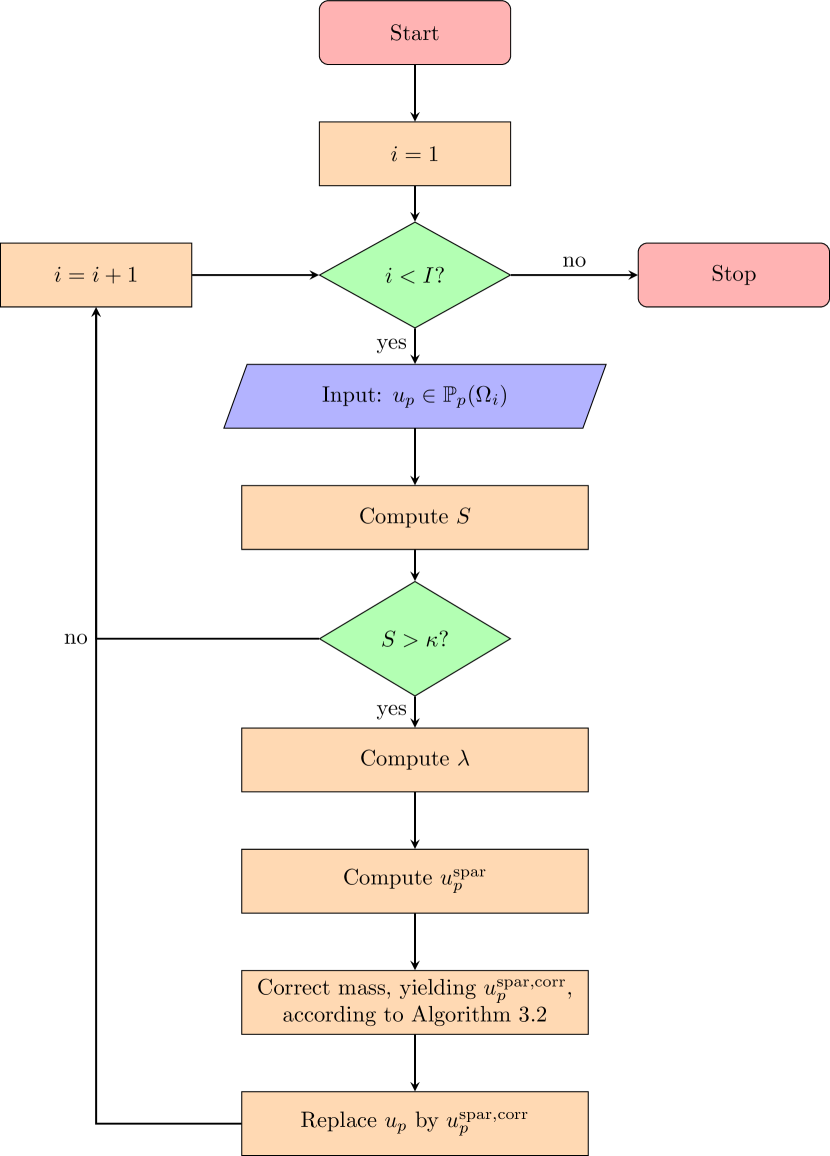
Figure 5: Flowchart describing $\ell^{1}$ regularization with mass correction. The procedure is described for a fixed time and includes the loop over all $I$ elements.

4 Numerical tests

We now numerically demonstrate the application of $\ell^{1}$ regularization (with and without mass correction) to a nodal DG method for the inviscid Burgers’ equation, the linear advection equation, and a nonlinear system of conservation laws. Our results show that $\ell^{1}$ regularization provides increased accuracy of the numerical solutions. In all numerical tests, we use a PA operator of third order and choose the same parameters as before, i.e., $\lambda_{\text{max}}=4\cdot 10^{2}$, $K=400$, $\beta=20$, $\alpha=0.0001$, and $tol=0.001$. We have made no effort to optimize these parameters.

4.1 Inviscid Burgers’ equation

We start our numerical investigation by considering the inviscid Burgers’ equation

$$\partial_{t}u+\partial_{x}\left(\frac{u^{2}}{2}\right)=0$$ (60)

on $\Omega=[0,2]$ with initial condition

$$u(0,x)=u_{0}(x)=\sin\left(\pi x\right)$$ (61)

and periodic boundary conditions. For this test case, a shock discontinuity develops in the solution at $x=1$.

In the subsequent numerical tests, the usual local Lax–Friedrichs flux

$$f^{\mathrm{num}}(u_{-},u_{+})=\frac{1}{2}\left(f(u_{+})+f(u_{-})\right)-\frac{{\alpha_{\mathrm{max}}}}{2}\left(u_{+}-u_{-}\right)$$ (62)

with maximum characteristic speed $\alpha_{\mathrm{max}}=\max\{|u_{+}|,|u_{-}|\}$ is utilized. Further, we use the third order explicit strong stability preserving Runge–Kutta method with three stages (SSPRK(3,3)) for time integration (see [70]) and choose the ramp parameter ${\kappa=0.8}$ in (31).

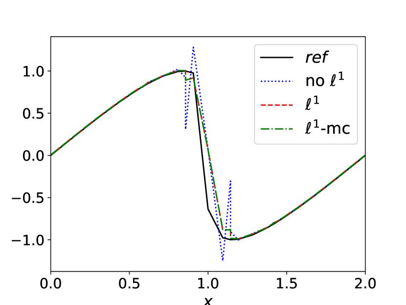
(a) Solution for $p=4$.

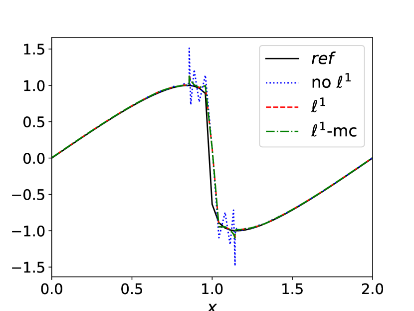
(b) Solution for $p=10$.

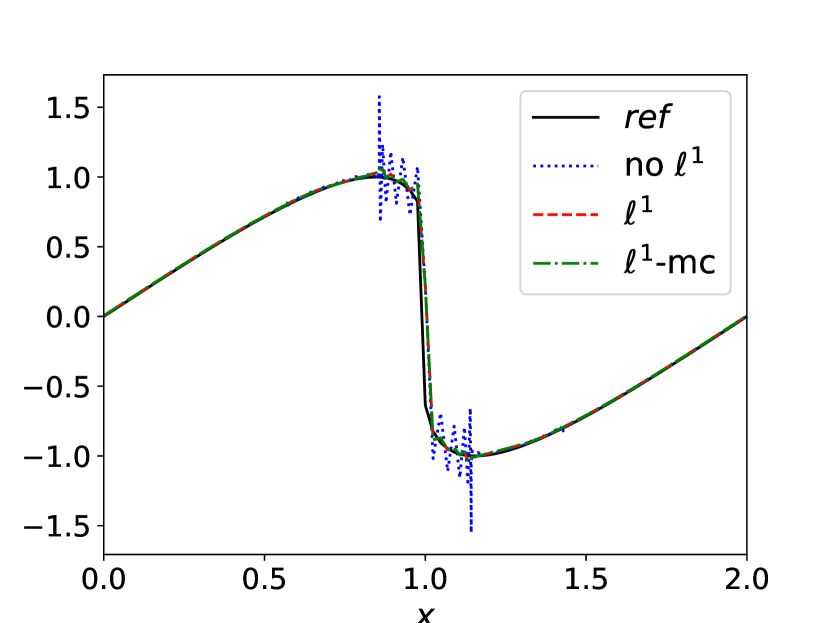
(c) Solution for $p=18$.

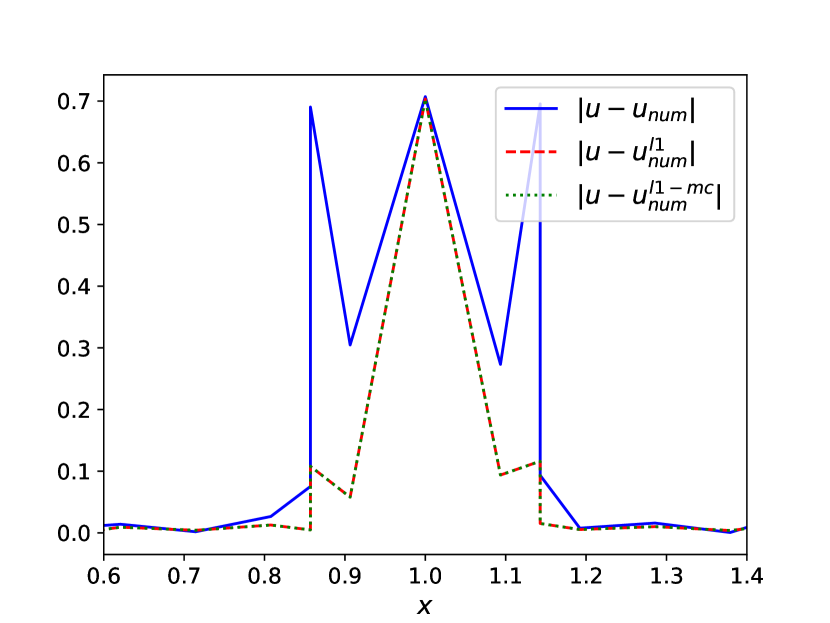
(d) Errors for $p=4$.

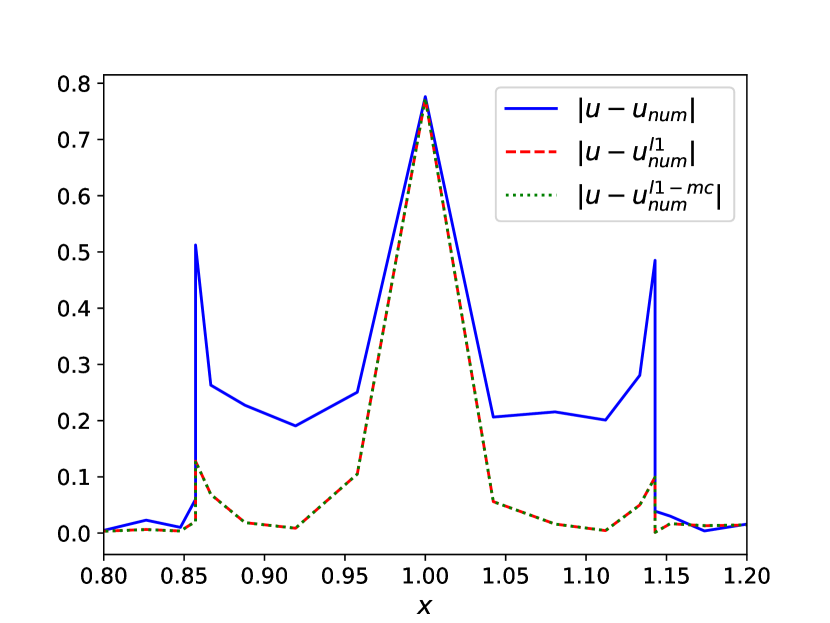
(e) Errors for $p=10$.

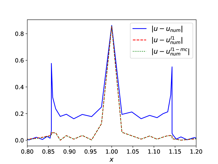
(f) Errors for $p=18$.

Figure 6: Numerical solutions (and their pointwise errors) at $t=0.345$ by the DG method for $I=7$ elements and polynomial orders $p=4,10,18$. Without $\ell^{1}$ regularization (straight blue line), with $\ell^{1}$ regularization (dashed red line), and with $\ell^{1}$ regularization and mass correction (dash-dotted green line).

Figure 6 illustrates the numerical solutions of the above test problem at time $t=0.345$. In Figure 6(a) a polynomial degree of $p=4$ was used on $I=7$ equidistant elements, while in Figure 6(b) a polynomial degree of $p=10$ was used on $I=7$ equidistant elements and in Figure 6(c) a polynomial degree of $p=18$ was used on $I=7$ equidistant elements. All tests show spurious oscillations for the numerical solution without $\ell^{1}$ regularization. These oscillations are significantly reduced when $\ell^{1}$ regularization is applied to the numerical solution after every time step. As a consequence, Figures 6(d), 6(e), 6(f) illustrate how the pointwise error of the numerical solutions utilizing $\ell^{1}$ regularization (with and without mass correction) is reduced compared to the numerical solution without $\ell^{1}$ regularization. Again, considering an odd function, only very slight differences are observed between $\ell^{1}$ regularization with and without mass correction. The reference solution $u$ was computed using characteristic tracing.

We now extend the above error analysis for the $\ell^{1}$ regularization. Table 2 lists the different common types of errors of the numerical solution for the above test problem (60), (61) and a varying polynomial degree $p$ as well as a varying number of equidistant elements $I$. Here we consider the global errors with respect to the discrete $\underline{\underline{M}}\,$-norm, as defined in (8), approximating the continuous $L^{2}$-norm and the discrete $1$-norm, given by $\mathinner{\!\left\lVert u_{p}\right\rVert}_{1}=\sum_{k=0}^{p}\omega_{k}\left|u_{p}(x_{k})\right|=\left\langle{\underline{1},\,\left|\underline{u}\right|}\right\rangle_{\underline{\underline{M}}\,}$ on the reference element. The discrete $\infty$-norm is given by $\mathinner{\!\left\lVert u_{p}\right\rVert}_{\infty}=\max_{k=0,\dots,p}|u_{p}(x_{k})|$. For the discrete $\underline{\underline{M}}\,$-norm and discrete $1$-norm, the global norms are defined by summing up over the weighted local norms, i.e.,

$$\mathinner{\!\left\lVert u_{\mathrm{num}}\right\rVert}^{2}=\sum_{i=1}^{I}\ \frac{\left|\Omega_{i}\right|}{2}\ \mathinner{\!\left\lVert u_{p}^{(i)}\right\rVert}^{2},$$ (63)

where $u_{p}^{(i)}$ denotes the numerical solution (polynomial approximation) on the $i$th element $\Omega_{i}$.

		$\mathinner{\!\left\lVert\cdot\right\rVert}_{M}$-error			$\mathinner{\!\left\lVert\cdot\right\rVert}_{1}$-error			$\mathinner{\!\left\lVert\cdot\right\rVert}_{\infty}$-error
$p$	$I$	no $\ell^{1}$	$\ell^{1}$	$\ell^{1}$-mc	no $\ell^{1}$	$\ell^{1}$	$\ell^{1}$-mc	no $\ell^{1}$	$\ell^{1}$	$\ell^{1}$-mc
3	15	1.5e-2	3.3e-2	3.3e-2	1.2e-2	2.2e-1	1.2e-2	1.7e-1	3.3e-1	3.3e-1
	31	1.5e-2	2.0e-2	2.0e-2	1.1e-2	1.2e-2	1.2e-2	2.2e-1	3.2e-1	3.2e-1
	63	1.9e-2	2.4e-2	2.4e-2	1.1e-2	1.1e-2 ✓	1.1e-2	3.6e-1	5.6e-1	5.6e-1
	127	3.3e-2	2.7e-2 ✓	2.7e-2	1.3e-2	1.1e-2 ✓	1.1e-2	1.4e-0	8.3e-1 ✓	8.3e-1
4	15	7.0e-2	5.9e-2 ✓	5.9e-2	3.9e-2	2.7e-2 ✓	2.7e-2	7.6e-1	7.5e-1 ✓	7.5e-1
	31	5.5e-2	4.6e-2 ✓	4.6e-2	2.4e-2	1.7e-2 ✓	1.7e-2	8.7e-1	8.6e-1 ✓	8.6e-1
	63	4.3e-2	3.9e-2 ✓	3.9e-2	1.6e-2	1.3e-2 ✓	1.3e-2	1.0	1.0e-0 ✓	1.0e-0
	127	3.8e-2	3.6e-2 ✓	3.6e-2	1.2e-2	1.2e-2 ✓	1.1e-2	1.4	1.3e-0 ✓	1.3e-0
5	15	1.6e-2	1.5e-2 ✓	1.5e-2	1.2e-2	1.2e-2 ✓	1.2e-2	2.5e-1	1.9e-1 ✓	1.7e-1
	31	2.0e-2	1.4e-2 ✓	1.3e-2	1.3e-2	1.0e-2 ✓	1.0e-2	5.3e-1	2.6e-1 ✓	2.5e-1
	63	7.3e-2	1.9e-2 ✓	1.6e-2	2.2e-2	1.0e-2 ✓	1.0e-2	3.6e-0	5.3e-1 ✓	4.3e-1
	127	NaN	2.7e-2 !	2.2e-2	NaN	1.0e-2 !	1.0e-2	NaN	1.1e-0 !	9.1e-1
6	15	5.9e-2	5.2e-2 ✓	5.2e-2	3.2e-2	2.3e-2	2.3e-2	8.1e-1	8.0e-1 ✓	8.0e-1
	31	4.7e-2	4.3e-2 ✓	4.3e-2	2.0e-2	1.6e-2 ✓	1.6e-2	9.6e-1	9.5e-1 ✓	9.5e-1
	63	3.9e-2	3.7e-2 ✓	3.6e-2	1.2e-2	1.2e-2 ✓	1.2e-2	1.2e-0	1.1e-0 ✓	1.1e-0
	127	NaN	3.4e-2 !	3.2e-2	NaN	1.1e-2 !	1.1e-2	NaN	1.3e-0 !	1.3e-0
7	15	1.7e-2	1.8e-2	1.8e-2	1.4e-2	1.2e-2 ✓	1.2e-2	2.2e-1	2.7e-1	2.8e-1
	31	2.5e-2	1.7e-2 ✓	1.8e-2	1.5e-2	1.1e-2 ✓	1.1e-2	7.0e-1	3.8e-1 ✓	4.0e-1
	63	5.0e-1	2.1e-2 ✓	2.2e-2	1.4e-1	1.0e-2 ✓	1.0e-2	1.1e+1	6.9e-1 ✓	7.5e-1
	127	2.8e-2	2.5e-2 ✓	2.5e-2	1.0e-2	1.0e-2 ✓	1.0e-2	1.3e-0	1.2e-0 ✓	1.2e-0
8	15	5.9e-2	4.9e-2 ✓	4.9e-2	3.2e-2	2.1e-2 ✓	2.1e-2	9.9e-1	8.6e-1 ✓	8.6e-1
	31	4.5e-2	4.0e-2 ✓	4.0e-2	1.9e-2	1.4e-2 ✓	1.4e-2	1.0e-0	1.0e-0 ✓	1.0e-0
	63	3.8e-2	3.6e-2 ✓	3.7e-2	1.2e-2	1.2e-2 ✓	1.2e-2	1.4e-0	1.3e-0 ✓	1.3e-0
	127	1.5e-1	3.2e-2 ✓	3.1e-2	3.1e-2	1.1e-2 ✓	1.1e-2	6.9e-0	1.4e-0 ✓	1.4e-0
9	15	2.0e-2	1.9e-2 ✓	1.8e-2	1.5e-2	1.3e-2 ✓	1.3e-2	4.5e-1	3.0e-1 ✓	2.9e-1
	31	7.8e-2	1.9e-2 ✓	1.8e-2	2.5e-2	1.1e-2 ✓	1.1e-2	4.5e-0	4.5e-1 ✓	4.1e-1
	63	NaN	2.3e-2 !	2.2e-2	NaN	1.0e-2 !	1.0e-2	NaN	9.0e-1 !	8.3e-1
	127	NaN	2.7e-2 !	2.8e-2	NaN	1.0e-2 !	1.0e-2	NaN	1.4e-0 !	1.4e-0

Table 2: Errors of the numerical solutions without and with $\ell^{1}$ regularization. In cases where the error value is NaN, the numerical solution broke down before the final time was reached. “no $\ell^{1}$” refers to the underlying DG method without $\ell^{1}$ regularization, “$\ell^{1}$” refers to the DG method with $\ell^{1}$ regularization, and “$\ell^{1}$-mc” refers to the DG method with $\ell^{1}$ regularization and additional mass correction.

Table 2 demonstrates that for almost all these norms as well as combinations of polynomial degrees $p=4,5,6,7,8,9$ and number of elements $I=15,32,63,127$, the numerical solution with $\ell^{1}$ regularization is more accurate than the numerical solution without $\ell^{1}$ regularization. Further, we observe just a slight difference in accuracy for $\ell^{1}$ regularization with and without mass correction. See, for instance, $p=5$ in Table 2. We only utilize odd number of elements, so that the shock discontinuity arises in the interior of an element. By using an even number of elements, on the other hand, the shock would arise at the interface between two elements and the error analysis of the $\ell^{1}$ regularization would be blurred by the dissipation added by the numerical flux.

In Table 2, all cases where the accuracy is increased or remains the same by applying $\ell^{1}$ regularization are flagged with a checkmark. It should be stressed that no effort was made to optimize the parameters in the $\ell^{1}$ regularization. In particular, the parameters in the $\ell^{1}$ regularization have not been adapted to the specific choice of the polynomial degree $p$, the number of elements $I$, or the number of time steps used in the solver. We think that by further investigations of the parameters in the $\ell^{1}$ regularization, all above errors could be further reduced.

Finally, special attention should be given to the cases flagged by an exclamation mark (!). In these cases, the numerical solver without $\ell^{1}$ regularization broke down completely. Yet, when $\ell^{1}$ regularization was applied, the same computations yielded fairly accurate numerical solutions.

4.2 Linear advection equation

The prior test case featured a shock discontinuity and might not fully reflect the behavior of the $\ell^{1}$ regularized DG method in smooth regions. Note that for the underlying spectral DG method used in this work, given $p+1$ nodes, the optimal order of convergence is $p+1$ in sufficiently smooth regions. Especially in smooth regions, it is desirable that the convergence properties of the underlying method are preserved when using the $\ell^{1}$ regularization method. Convergence of the $\ell^{1}$ regularized DG method, however, also depends on the convergence of the PA operator. In all numerical tests presented in this work, a PA operator of order three, i.e., $L_{3}$, is used. Hence, if falsely activated (false positive; see Remark 3) by the discontinuity sensor (30), $\ell^{1}$ regularization might affect the order of convergence of the underlying method in smooth regions. In our numerical tests, we observed the sensor to be fairly reliable for sufficient resolution, and $\ell^{1}$ regularization did not get activated in smooth regions.

To investigate this potential drawback and demonstrate the reliability of the $\ell^{1}$ regularized DG method in smooth regions, we now consider the linear advection equation

$$\partial_{t}u+\partial_{x}u=0$$ (64)

on $\Omega=[0,2]$ with initial condition

$$u(0,x)=\sin\left(2\pi x\right)$$ (65)

and periodic boundary conditions, which provides a smooth solution for all times. Table 3 lists comparative errors for DG with and without the $\ell^{1}$ regularization and with the additional mass conservation correction term at time $T=2$.

		$\mathinner{\!\left\lVert\cdot\right\rVert}_{M}$-error			$\mathinner{\!\left\lVert\cdot\right\rVert}_{1}$-error			$\mathinner{\!\left\lVert\cdot\right\rVert}_{\infty}$-error
$p$	$I$	no $\ell^{1}$	$\ell^{1}$	$\ell^{1}$-mc	no $\ell^{1}$	$\ell^{1}$	$\ell^{1}$-mc	no $\ell^{1}$	$\ell^{1}$	$\ell^{1}$-mc
3	2	1.2e-0	1.2e-0	1.2e-0	1.5e-0	1.6e-0	1.6e-0	9.5e-1	9.8e-1	9.8e-1
	4	1.3e-1	4.4e-1	4.4e-1	1.4e-1	5.8e-1	5.8e-1	1.3e-1	4.1e-1	4.1e-1
	8	6.3e-3	6.3e-3	6.3e-3	7.0e-3	7.0e-3	7.0e-3	1.2e-2	1.2e-2	1.2e-2
	16	3.8e-4	3.8e-4	3.8e-4	3.8e-4	3.8e-4	3.8e-4	9.9e-4	9.9e-4	9.9e-4
4	2	3.4e-1	9.2e-1	9.2e-1	4.2e-1	9.7e-1	9.6e-1	3.8e-1	9.0e-1	8.8e-1
	4	7.8e-3	7.8e-3	7.8e-3	1.0e-2	1.0e-2	1.0e-2	1.2e-2	1.2e-2	1.2e-2
	8	4.2e-4	4.2e-4	4.2e-4	4.4e-4	4.4e-4	4.4e-4	1.2e-3	1.2e-3	1.2e-3
	16	1.3e-5	1.3e-5	1.3e-5	1.3e-5	1.3e-5	1.3e-5	4.4e-5	4.4e-5	4.4e-5
5	2	8.0e-2	1.0e-0	1.0e-0	1.0e-1	1.3e-0	1.3e-0	1.3e-1	8.4e-1	7.8e-1
	4	2.1e-3	2.1e-3	2.1e-3	2.3e-3	2.3e-3	2.3e-3	5.3e-3	5.3e-3	5.3e-3
	8	2.8e-5	2.8e-5	2.8e-5	2.9e-5	2.9e-5	2.9e-5	7.7e-5	7.7e-5	7.7e-5
	16	1.2e-6	1.2e-6	1.2e-6	1.5e-6	1.5e-6	1.5e-6	1.6e-6	1.6e-6	1.6e-6
6	2	2.1e-2	9.9e-1	9.9e-1	2.5e-2	1.1e-0	1.1e-0	5.1e-2	9.9e-1	9.9e-1
	4	7.5e-5	7.5e-5	7.5e-5	8.0e-5	8.0e-5	8.0e-5	1.8e-4	1.8e-4	1.8e-4
	8	6.0e-6	6.0e-6	6.0e-6	7.6e-6	7.6e-6	7.6e-6	7.5e-6	7.5e-6	7.5e-6
	16	7.3e-7	7.3e-7	7.3e-7	9.4e-7	9.4e-7	9.4e-7	7.4e-7	7.4e-7	7.4e-7
7	2	2.0e-3	2.0e-3	2.0e-3	2.0e-3	2.0e-3	2.0e-3	6.4e-3	6.4e-3	6.4e-3
	4	3.9e-5	3.9e-5	3.9e-5	4.9e-5	4.9e-5	4.9e-5	6.8e-5	6.8e-5	6.8e-5
	8	3.9e-6	3.9e-6	3.9e-6	5.0e-6	5.0e-6	5.0e-6	4.1e-6	4.1e-6	4.1e-6
	16	4.9e-7	4.9e-7	4.9e-7	6.3e-7	6.3e-7	6.3e-7	4.9e-7	4.9e-7	4.9e-7

Table 3: $u(0,x)=\sin\left(2\pi x\right)$. Errors of the numerical solutions without and with $\ell^{1}$ regularization. “no $\ell^{1}$” refers to the underlying DG method without $\ell^{1}$ regularization, “$\ell^{1}$” refers to the DG method with $\ell^{1}$ regularization, and “$\ell^{1}$-mc” refers to the DG method with $\ell^{1}$ regularization and additional mass correction.

Our results indicate that $\ell^{1}$ regularization is only activated, and thus affects convergence of the underlying method, if the solution is heavily underresolved. This can be noted in Table 3 from $p=3$ and $N=2,4$ as well as $p=4,5,6$ and $N=2$. For $p=7$, even $N=2$ provides sufficient resolution and the $\ell^{1}$ regularization is not activated. For all numerical solutions, using at least $N=8$ elements, $\ell^{1}$ regularization does not affect accuracy and convergence of the underlying method in smooth regions. Finally, we note that in the cases where the numerical solution is heavily underresolved and $\ell^{1}$ regularization is activated, $\ell^{1}$ regularization with additional mass correction (l1-mc) provides slightly more accurate solutions than $\ell^{1}$ regularization without mass correction (l1). Finally, we note that because the $\ell^{1}$ regularization is only activated in elements containing discontinuities, the efficiency of our new method is comparable to the underlying DG method. Moreover, as in [24], we observed that for our specific set of test problems we were able to maintain stability for time step sizes larger than the standard CFL constraints suggest. Theoretical justification for this will be part of future investigations.

4.3 Systems of conservation laws

We now extend our hybrid $\ell^{1}$ regularized DG method to the nonlinear system of conservation laws

$$\partial_{t}\begin{pmatrix}u_{0}\\ u_{1}\end{pmatrix}+\frac{1}{2}\partial_{x}\begin{pmatrix}u_{0}^{2}+u_{1}^{2}\\ 2u_{0}u_{1}\end{pmatrix}=0$$ (66)

in the domain $\Omega=[0,2]$. System (66) originates from a truncated polynomial chaos approach for Burgers’ equation with uncertain initial condition [71, 72, 73]. In this context, $u_{0}$ models the expected value of the numerical solution while $u_{1}^{2}$ approximates the variance. For the spatial semidiscretization of (66) we follow [73, 10], where a skew-symmetric formulation

$$\underline{\dot{u_{k}}}= -\frac{1}{3}\sum_{i,j=0}^{1}\langle\varphi_{i}\varphi_{j}\varphi_{k}\rangle\left(\underline{\underline{D}}\,\underline{u_{i}u_{j}}+\underline{\underline{u_{j}}}\,^{*}\underline{\underline{D}}\,\underline{u_{i}}\right)$$ (67)

$$-\underline{\underline{M}}\,^{-1}\underline{\underline{R}}\,^{T}\underline{\underline{B}}\,\left(\underline{f_{k}}^{\mathrm{num}}-\sum_{i,j=0}^{1}\langle\varphi_{i}\varphi_{j}\varphi_{k}\rangle\left(\frac{1}{3}\underline{\underline{R}}\,\underline{u_{i}u_{j}}+\frac{1}{6}\left(\underline{\underline{R}}\,\underline{u_{i}}\right)\circ\left(\underline{\underline{R}}\,\underline{u_{j}}\right)\right)\right)$$

was proposed. Here $\langle\varphi_{i}\varphi_{j}\varphi_{k}\rangle$ denotes the triple product $\int\varphi_{i}(\xi)\varphi_{j}(\xi)\varphi_{k}(\xi)\omega(\xi)\operatorname{d\!}\xi$, $\circ$ denotes the componentwise (Hadamard) product of two vectors, and $\{\varphi_{k}\}$ is a set of orthogonal polynomials (typically Hermite polynomials are used).

It was further proved in [73] that (67) yields an entropy conservative semidiscretization when combined with the entropy conservative flux $\underline{f_{k}}^{\mathrm{num}}$ presented in [73]. An entropy stable semidiscretization is thus obtained by adding a dissipative term $-\underline{\underline{Q}}\,(\underline{u_{k}}_{+}-\underline{u_{k}}_{-})$ to the entropy conservative flux. Here we simply use a local Lax–Friedrichs type dissipation matrix

$$\underline{\underline{Q}}\,=\frac{{\alpha}}{2}\,\underline{\underline{\operatorname{I}}}\,\quad\text{with}\quad{\alpha}=\max\mathinner{\left\{\mathinner{\!\left\lvert{\alpha}(-)\right\rvert},\mathinner{\!\left\lvert{\alpha}(+)\right\rvert}\right\}},$$ (68)

where $\mathinner{\!\left\lvert{\alpha}(\pm)\right\rvert}$ is the largest absolute value of all eigenvalues of the Jacobian $f^{\prime}(u(\pm))$.

Even though the skew-symmetric formulation (67) combined with an appropriate numerical flux yields an entropy stable scheme, this test case demonstrates that additional regularization is still necessary to obtain reasonable numerical solutions. This was, for instance, stressed in [10]. Here we demonstrate how $\ell^{1}$ regularization enhances the numerical solution for the nonlinear system (66) with periodic boundary conditions and initial condition

$$u_{0}(x,0) =1+\left\{\begin{array}[]{lll}e\cdot\exp\left(-\frac{r^{2}}{r^{2}-(x-0.5)^{2}}\right)&,&\text{if }|x-0.5|<r,\\ 0&,&\text{if }|x-0.5|\geq r,\end{array}\right.$$ (71)

$$u_{1}(x,0) =\left\{\begin{array}[]{lll}e\cdot\exp\left(-\frac{r^{2}}{r^{2}-(x-0.5)^{2}}\right)&,&\text{if }|x-0.5|<r,\\ 0&,&\text{if }|x-0.5|\geq r,\end{array}\right.$$ (74)

where $r=0.5$.

For the more general case of systems of conservation laws, we propose a straightforward extension of our $\ell^{1}$ regularization technique. Specifically, the PA sensor (30) is applied to every conserved variable $u_{k}$ separately and, once a discontinuity is detected, $\ell^{1}$ regularization (27) is performed for the respective variable. For this test case, the ramp parameter in (31) has been chosen as $\kappa=0.9$.

Figure 7 illustrates the results of $\ell^{1}$ regularization (with and without mass correction) for the above described test case and for an entropy stable numerical flux. In all subsequent tests $I=100$ equidistant elements and a polynomial basis of degree $p=6$ have been used. Further, for the $\ell^{1}$ regularization, the same parameters as before have been used, i.e., $\lambda_{\text{max}}=4\cdot 10^{2}$, $K=400$, $\beta=20$, $\alpha=0.0001$, and $tol=0.001$.

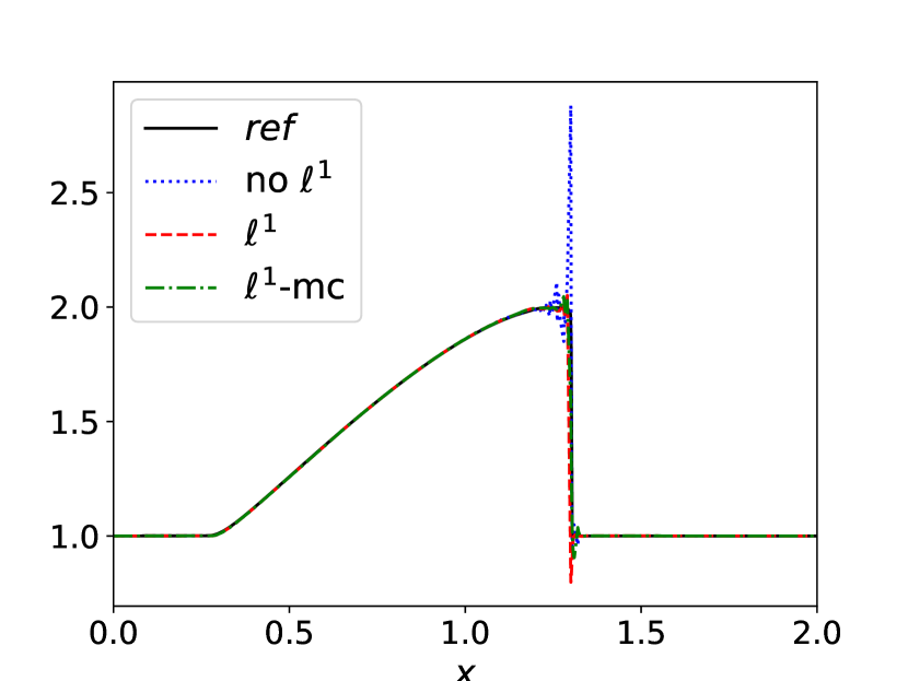
(a) Coefficient $u_{0}$.

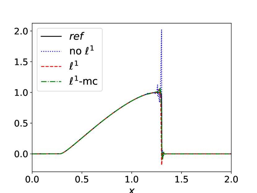
(b) Coefficient $u_{1}$.

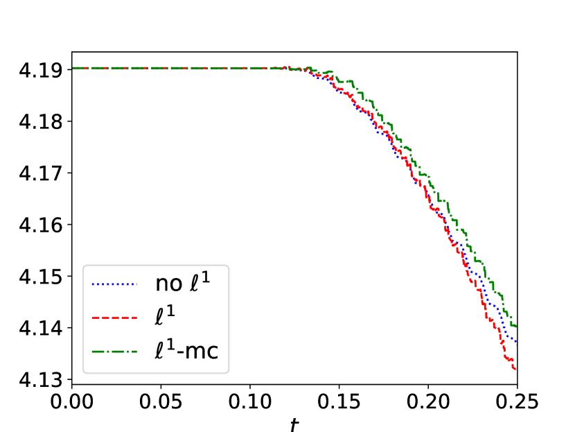
(c) Energy over time.

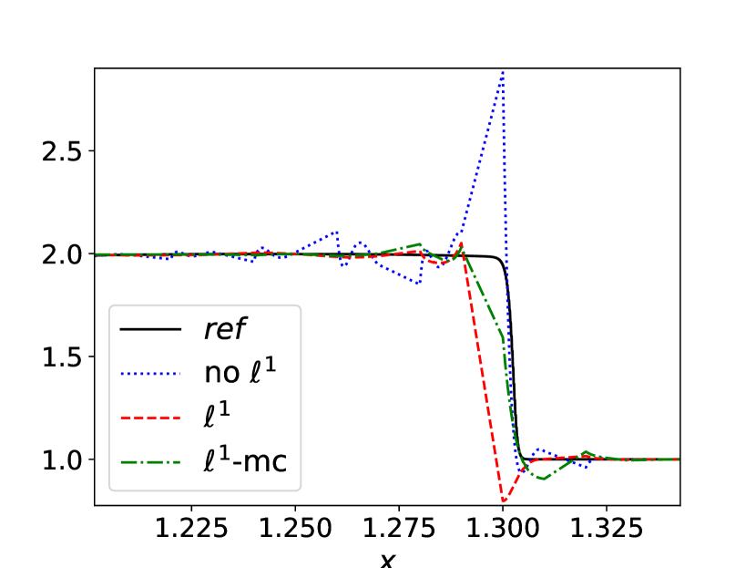
(d) Coefficient $u_{0}$.

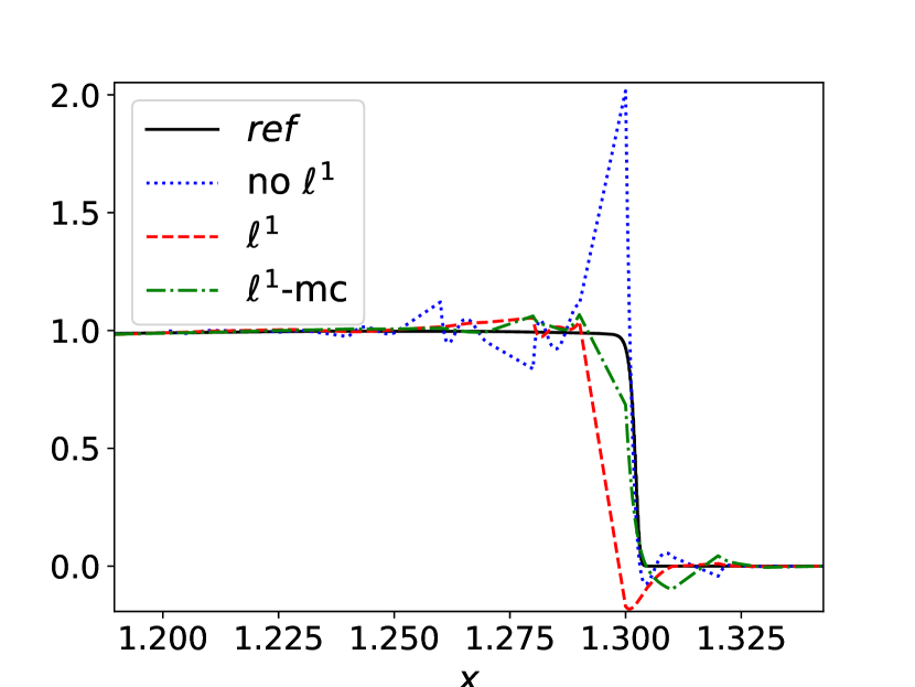
(e) Coefficient $u_{1}$.

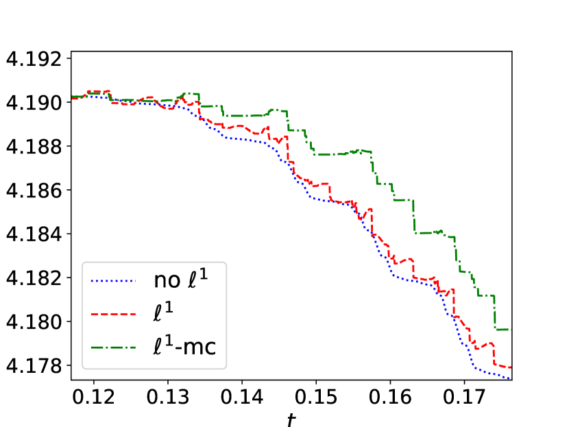
(f) Energy over time.

Figure 7: Components of the numerical solutions at $t=0.25$ by the DG method for $I=100$ elements and polynomial degree $p=6$. Without $\ell^{1}$ regularization (straight blue line), with $\ell^{1}$ regularization (dashed red line), and with $\ell^{1}$ regularization and mass correction (dash-dotted green line). In all tests an entropy stable numerical flux has been used.

(a) Coefficient $u_{0}$.

(b) Coefficient $u_{1}$.

(c) Energy over time.

(d) Coefficient $u_{0}$.

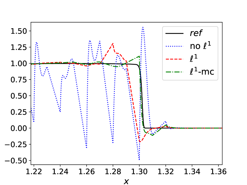
(e) Coefficient $u_{1}$.

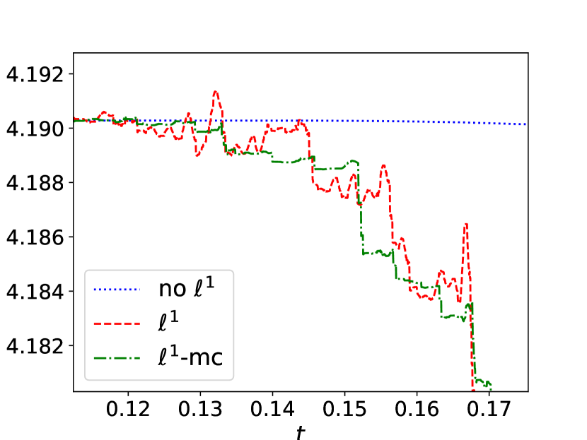
(f) Energy over time.

Figure 8: Components of the numerical solutions at $t=0.25$ by the DG method for $I=100$ elements and polynomial degree $p=6$. Without $\ell^{1}$ regularization (straight blue line), with $\ell^{1}$ regularization (dashed red line), and with $\ell^{1}$ regularization and mass correction (dash-dotted green line). In all tests an entropy conservative numerical flux has been used.

Note that while the numerical solution without $\ell^{1}$ regularization shows heavy oscillations in both components, the numerical solution with $\ell^{1}$ regularization provides a significantly sharper profile. Further, by consulting Figures 7(d) and 7(e), it should be stressed that only $\ell^{1}$ regularization with additional mass correction is able to capture the exact shock location. Due to missing conservation, $\ell^{1}$ regularization without mass correction results in a slightly wrong location for the shock. Finally, Figures 7(c) and 7(f) illustrate the energy of the different methods over time. We note from these figures that $\ell^{1}$ regularization (with and without mass correction) slightly increase the energy in this test case.

In order to further emphasize the effect of $\ell^{1}$ regularization (with and without mass correction), similar results using an entropy conservative numerical flux at the interfaces between elements are shown in Figure 8. Once again, $\ell^{1}$ regularization is demonstrated to improve the numerical solution. The best results are obtained when $\ell^{1}$ regularization is combined with mass correction. In particular, only $\ell^{1}$ regularization with additional mass correction is able to accurately capture the shock at the right location. Finally, consulting Figures 8(c) and 8(f), $\ell^{1}$ regularization decreases the energy overall. Yet, it is demonstrated once more that an entropy inequality is not satisfied by $\ell^{1}$ regularization, i.e., the energy might increase as well as decrease by utilizing $\ell^{1}$ regularization. Thus, future work will focus on incorporating energy stability (as well as other properties like TVD or positivity) by additional constraints in the minimization problem (26).

5 Concluding remarks

We have presented a novel approach to shock capturing by $\ell^{1}$ regularization using SE approximations. Our work not only is distinguished from previous studies [20, 21, 22, 23, 25] by focusing on discontinuous solutions but further by promoting sparsity of the jump function instead of the numerical solution itself. By approximating the jump function with the (high order) PA operator, we help to eliminate the staircase effect that arises for classical TV operators. Our results demonstrate that it is possible to efficiently implement a method that yields increased accuracy and better resolves (shock) discontinuities. In particular, no additional time step restrictions are introduced, in contrast to artificial viscosity methods when no care is taken in their construction. This approach for solving numerical conservation laws was first used in [24], where the Lax–Wendroff scheme and Chebyshev and Fourier spectral methods were used as the numerical PDE solver. Our method improves upon the approach in [24] in two ways. First, we employ the SE approximation for solving the conservation law, which allows element-to-element variations in the optimization problem. In particular, $\ell^{1}$ regularization is only activated in troubled elements, which enhances accuracy and efficiency of the method. Second, in the process we proposed a novel discontinuity sensor based on PA operators of increasing orders, which is able to flag troubled elements as well as to steer the amount of regularization introduced by the sparse reconstruction.

Numerical tests demonstrate the method using a nodal collocation-type discontinuous Galerkin method for the inviscid Burgers’ equation, the linear advection equation, and a nonlinear system of conservation laws. Our results show that the method yields improved accuracy and robustness.

No effort was made in our study to optimize any of the parameters involved in solving the optimization problem. This will be addressed in future work, along with the possibility to include additional constraints (e.g., for entropy, TVD, and positivity constraints), since preliminary results presented here are encouraging. The generalization of the approach itself to higher dimensions is straightforward and has already been demonstrated in [24]. Of interest, however, would be the extension of the proposed approach to other classes of methods, such as finite volume methods. We believe $\ell^{1}$ regularization might be an important ingredient to make high order methods viable in several research applications.

References

- Liu et al. [2006] Y. Liu, M. Vinokur, Z. Wang, Spectral difference method for unstructured grids i: basic formulation, Journal of Computational Physics 216 (2006) 780–801.
- Wang et al. [2007] Z. Wang, Y. Liu, G. May, A. Jameson, Spectral difference method for unstructured grids ii: extension to the Euler equations, Journal of Scientific Computing 32 (2007) 45–71.
- Hesthaven and Warburton [2007] J. S. Hesthaven, T. Warburton, Nodal discontinuous Galerkin methods: algorithms, analysis, and applications, Springer Science & Business Media, 2007.
- Huynh [2007] H. T. Huynh, A flux reconstruction approach to high-order schemes including discontinuous Galerkin methods, AIAA paper 4079 (2007) 2007.
- VonNeumann and Richtmyer [1950] J. VonNeumann, R. D. Richtmyer, A method for the numerical calculation of hydrodynamic shocks, Journal of applied physics 21 (1950) 232–237.
- Jameson et al. [1981] A. Jameson, W. Schmidt, E. Turkel, Numerical solution of the Euler equations by finite volume methods using Runge Kutta time stepping schemes, in: 14th fluid and plasma dynamics conference, 1981, p. 1259.
- Persson and Peraire [2006] P.-O. Persson, J. Peraire, Sub-cell shock capturing for discontinuous Galerkin methods, in: 44th AIAA Aerospace Sciences Meeting and Exhibit, 2006, p. 112.
- Klöckner et al. [2011] A. Klöckner, T. Warburton, J. S. Hesthaven, Viscous shock capturing in a time-explicit discontinuous Galerkin method, Mathematical Modelling of Natural Phenomena 6 (2011) 57–83.
- Nordström [2006] J. Nordström, Conservative finite difference formulations, variable coefficients, energy estimates and artificial dissipation, Journal of Scientific Computing 29 (2006) 375–404.
- Ranocha et al. [2018] H. Ranocha, J. Glaubitz, P. Öffner, T. Sonar, Stability of artificial dissipation and modal filtering for flux reconstruction schemes using summation-by-parts operators, Applied Numerical Mathematics 128 (2018) 1–23.
- Glaubitz et al. [2019] J. Glaubitz, A. Nogueira, J. Almeida, R. Cantão, C. Silva, Smooth and compactly supported viscous sub-cell shock capturing for discontinuous Galerkin methods, Journal of Scientific Computing 79 (2019) 249–272.
- Hesthaven and Kirby [2008] J. Hesthaven, R. Kirby, Filtering in Legendre spectral methods, Mathematics of Computation 77 (2008) 1425–1452.
- Glaubitz et al. [2018] J. Glaubitz, P. Öffner, T. Sonar, Application of modal filtering to a spectral difference method, Mathematics of Computation 87 (2018) 175–207.
- Tadmor [1990] E. Tadmor, Shock capturing by the spectral viscosity method, Computer Methods in Applied Mechanics and Engineering 80 (1990) 197–208.
- Tadmor et al. [1993] E. Tadmor, M. Baines, K. Morton, Super viscosity and spectral approximations of nonlinear conservation laws (1993).
- Cockburn and Shu [1989] B. Cockburn, C.-W. Shu, Tvb runge-kutta local projection discontinuous galerkin finite element method for conservation laws. ii. general framework, Mathematics of computation 52 (1989) 411–435.
- Dervieux et al. [2003] A. Dervieux, D. Leservoisier, P.-L. George, Y. Coudière, About theoretical and practical impact of mesh adaptation on approximation of functions and PDE solutions, International journal for numerical methods in fluids 43 (2003) 507–516.
- Shu and Osher [1988] C.-W. Shu, S. Osher, Efficient implementation of essentially non-oscillatory shock-capturing schemes, Journal of computational physics 77 (1988) 439–471.
- Shu and Osher [1989] C.-W. Shu, S. Osher, Efficient implementation of essentially non-oscillatory shock-capturing schemes, ii, Journal of Computational Physics 83 (1989) 32–78.
- Schaeffer et al. [2013] H. Schaeffer, R. Caflisch, C. D. Hauck, S. Osher, Sparse dynamics for partial differential equations, Proceedings of the National Academy of Sciences 110 (2013) 6634–6639.
- Hou et al. [2015] T. Y. Hou, Q. Li, H. Schaeffer, Sparse+ low-energy decomposition for viscous conservation laws, Journal of Computational Physics 288 (2015) 150–166.
- Lavery [1989] J. Lavery, Solution of steady-state one-dimensional conservation laws by mathematical programming, SIAM Journal on Numerical Analysis 26 (1989) 1081–1089.
- Lavery [1991] J. E. Lavery, Solution of steady-state, two-dimensional conservation laws by mathematical programming, SIAM Journal on Numerical Analysis 28 (1991) 141–155.
- Scarnati et al. [2017] T. Scarnati, A. Gelb, R. B. Platte, Using regularization to improve numerical partial differential equation solvers, Journal of Scientific Computing (2017) 1–28.
- Guermond et al. [2008] J.-L. Guermond, F. Marpeau, B. Popov, et al., A fast algorithm for solving first-order PDEs by l1-minimization, Communications in mathematical Sciences 6 (2008) 199–216.
- Archibald et al. [2016] R. Archibald, A. Gelb, R. B. Platte, Image reconstruction from undersampled Fourier data using the polynomial annihilation transform, Journal of Scientific Computing 67 (2016) 432–452.
- Archibald et al. [2005] R. Archibald, A. Gelb, J. Yoon, Polynomial fitting for edge detection in irregularly sampled signals and images, SIAM Journal on Numerical Analysis 43 (2005) 259–279.
- Wasserman et al. [2015] G. Wasserman, R. Archibald, A. Gelb, Image reconstruction from Fourier data using sparsity of edges, Journal of Scientific Computing 65 (2015) 533–552.
- Li et al. [2013] C. Li, W. Yin, H. Jiang, Y. Zhang, An efficient augmented Lagrangian method with applications to total variation minimization, Computational Optimization and Applications 56 (2013) 507–530.
- Sanders [2016] T. Sanders, Matlab imaging algorithms: Image reconstruction, restoration, and alignment, with a focus in tomography, 2016.
- Sanders et al. [2017] T. Sanders, A. Gelb, R. B. Platte, Composite sar imaging using sequential joint sparsity, Journal of Computational Physics 338 (2017) 357–370.
- Don et al. [2016] W.-S. Don, Z. Gao, P. Li, X. Wen, Hybrid compact-WENO finite difference scheme with conjugate Fourier shock detection algorithm for hyperbolic conservation laws, SIAM Journal on Scientific Computing 38 (2016) A691–A711.
- Kopriva [2009] D. A. Kopriva, Implementing spectral methods for partial differential equations: Algorithms for scientists and engineers, Springer Science & Business Media, 2009.
- Davis and Rabinowitz [2007] P. J. Davis, P. Rabinowitz, Methods of numerical integration, Courier Corporation, 2007.
- Gassner [2013] G. J. Gassner, A skew-symmetric discontinuous galerkin spectral element discretization and its relation to sbp-sat finite difference methods, SIAM Journal on Scientific Computing 35 (2013) A1233–A1253.
- Gassner [2014] G. J. Gassner, A kinetic energy preserving nodal discontinuous galerkin spectral element method, International Journal for Numerical Methods in Fluids 76 (2014) 28–50.
- Kopriva and Gassner [2014] D. A. Kopriva, G. J. Gassner, An energy stable discontinuous galerkin spectral element discretization for variable coefficient advection problems, SIAM Journal on Scientific Computing 36 (2014) A2076–A2099.
- Toro [2013] E. F. Toro, Riemann solvers and numerical methods for fluid dynamics: a practical introduction, Springer Science & Business Media, 2013.
- Allaneau and Jameson [2011] Y. Allaneau, A. Jameson, Connections between the filtered discontinuous Galerkin method and the flux reconstruction approach to high order discretizations, Computer Methods in Applied Mechanics and Engineering 200 (2011) 3628–3636.
- Yu and Wang [2013] M. Yu, Z. Wang, On the connection between the correction and weighting functions in the correction procedure via reconstruction method, Journal of Scientific Computing 54 (2013) 227–244.
- De Grazia et al. [2014] D. De Grazia, G. Mengaldo, D. Moxey, P. Vincent, S. Sherwin, Connections between the discontinuous Galerkin method and high-order flux reconstruction schemes, International journal for numerical methods in fluids 75 (2014) 860–877.
- Stefan et al. [2010] W. Stefan, R. A. Renaut, A. Gelb, Improved total variation-type regularization using higher order edge detectors, SIAM Journal on Imaging Sciences 3 (2010) 232–251.
- Archibald et al. [2009] R. Archibald, A. Gelb, R. Saxena, D. Xiu, Discontinuity detection in multivariate space for stochastic simulations, Journal of Computational Physics 228 (2009) 2676–2689.
- Jakeman et al. [2011] J. D. Jakeman, R. Archibald, D. Xiu, Characterization of discontinuities in high-dimensional stochastic problems on adaptive sparse grids, Journal of Computational Physics 230 (2011) 3977–3997.
- Candes et al. [2008] E. J. Candes, M. B. Wakin, S. P. Boyd, Enhancing sparsity by reweighted minimization, Journal of Fourier analysis and applications 14 (2008) 877–905.
- Gelb and Scarnati [2018] A. Gelb, T. Scarnati, Reducing effects of bad data using variance based joint sparsity recovery (2018). In preparation.
- Qiu and Shu [2005] J. Qiu, C.-W. Shu, A comparison of troubled-cell indicators for Runge–Kutta discontinuous Galerkin methods using weighted essentially nonoscillatory limiters, SIAM Journal on Scientific Computing 27 (2005) 995–1013.
- Bassi and Rebay [1995] F. Bassi, S. Rebay, Accurate 2d Euler computations by means of a high order discontinuous finite element method, in: Fourteenth International Conference on Numerical Methods in Fluid Dynamics, Springer, 1995, pp. 234–240.
- Jaffre et al. [1995] J. Jaffre, C. Johnson, A. Szepessy, Convergence of the discontinuous Galerkin finite element method for hyperbolic conservation laws, Mathematical Models and Methods in Applied Sciences 5 (1995) 367–386.
- Hartmann [2006] R. Hartmann, Adaptive discontinuous Galerkin methods with shock-capturing for the compressible Navier–Stokes equations, International Journal for Numerical Methods in Fluids 51 (2006) 1131–1156.
- Barter and Darmofal [2010] G. E. Barter, D. L. Darmofal, Shock capturing with PDE-based artificial viscosity for DGFEM: Part i. formulation, Journal of Computational Physics 229 (2010) 1810–1827.
- Feistauer and Kučera [2007] M. Feistauer, V. Kučera, On a robust discontinuous Galerkin technique for the solution of compressible flow, Journal of Computational Physics 224 (2007) 208–221.
- Guermond and Pasquetti [2008] J.-L. Guermond, R. Pasquetti, Entropy-based nonlinear viscosity for Fourier approximations of conservation laws, Comptes Rendus Mathematique 346 (2008) 801–806.
- Gelb and Tadmor [1999] A. Gelb, E. Tadmor, Detection of edges in spectral data, Applied and computational harmonic analysis 7 (1999) 101–135.
- Gelb and Tadmor [2000] A. Gelb, E. Tadmor, Detection of edges in spectral data ii. Nonlinear enhancement, SIAM Journal on Numerical Analysis 38 (2000) 1389–1408.
- Gelb and Tadmor [2006] A. Gelb, E. Tadmor, Adaptive edge detectors for piecewise smooth data based on the minmod limiter, Journal of Scientific Computing 28 (2006) 279–306.
- Gelb and Cates [2008] A. Gelb, D. Cates, Detection of edges in spectral data iii. Refinement of the concentration method, Journal of Scientific Computing 36 (2008) 1–43.
- Öffner et al. [2013] P. Öffner, T. Sonar, M. Wirz, Detecting strength and location of jump discontinuities in numerical data, Applied Mathematics 4 (2013) 1.
- Tadmor and Waagan [2012] E. Tadmor, K. Waagan, Adaptive spectral viscosity for hyperbolic conservation laws, SIAM Journal on Scientific Computing 34 (2012) A993–A1009.
- Archibald et al. [2008] R. Archibald, A. Gelb, J. Yoon, Determining the locations and discontinuities in the derivatives of functions, Applied Numerical Mathematics 58 (2008) 577–592.
- Huerta et al. [2012] A. Huerta, E. Casoni, J. Peraire, A simple shock-capturing technique for high-order discontinuous Galerkin methods, International Journal for Numerical Methods in Fluids 69 (2012) 1614–1632.
- Krivodonova et al. [2004] L. Krivodonova, J. Xin, J.-F. Remacle, N. Chevaugeon, J. E. Flaherty, Shock detection and limiting with discontinuous Galerkin methods for hyperbolic conservation laws, Applied Numerical Mathematics 48 (2004) 323–338.
- Glowinski and Marroco [1975] R. Glowinski, A. Marroco, Sur l’approximation, par éléments finis d’ordre un, et la résolution, par pénalisation-dualité d’une classe de problèmes de Dirichlet non linéaires, Revue française d’automatique, informatique, recherche opérationnelle. Analyse numérique 9 (1975) 41–76.
- Gabay and Mercier [1976] D. Gabay, B. Mercier, A dual algorithm for the solution of nonlinear variational problems via finite element approximation, Computers & Mathematics with Applications 2 (1976) 17–40.
- Glowinski and Le Tallec [1989] R. Glowinski, P. Le Tallec, Augmented Lagrangian and operator-splitting methods in nonlinear mechanics, volume 9, SIAM, 1989.
- Eckstein and Bertsekas [1992] J. Eckstein, D. P. Bertsekas, On the Douglas–Rachford splitting method and the proximal point algorithm for maximal monotone operators, Mathematical Programming 55 (1992) 293–318.
- Goldstein and Osher [2009] T. Goldstein, S. Osher, The split Bregman method for l1-regularized problems, SIAM journal on imaging sciences 2 (2009) 323–343.
- Hewitt and Hewitt [1979] E. Hewitt, R. E. Hewitt, The Gibbs-Wilbraham phenomenon: an episode in Fourier analysis, Archive for history of Exact Sciences 21 (1979) 129–160.
- Randall [1992] J. L. Randall, Numerical methods for conservation laws, Lectures in Mathematics ETH Zürich (1992).
- Gottlieb and Shu [1998] S. Gottlieb, C.-W. Shu, Total variation diminishing Runge–Kutta schemes, Mathematics of computation of the American Mathematical Society 67 (1998) 73–85.
- Pettersson et al. [2009] P. Pettersson, G. Iaccarino, J. Nordström, Numerical analysis of the Burgers’ equation in the presence of uncertainty, Journal of Computational Physics 228 (2009) 8394–8412.
- Pettersson et al. [2015] M. P. Pettersson, G. Iaccarino, J. Nordström, Polynomial chaos methods for hyperbolic partial differential equations: Numerical techniques for fluid dynamics problems in the presence of uncertainties, Springer, 2015.
- Öffner et al. [2018] P. Öffner, J. Glaubitz, H. Ranocha, Stability of correction procedure via reconstruction with summation-by-parts operators for burgers’ equation using a polynomial chaos approach, ESAIM: Mathematical Modelling and Numerical Analysis 52 (2018) 2215–2245.