Hybrid Transceiver Optimization for Multi-Hop Communications

Abstract

Multi-hop communication with the aid of large-scale antenna arrays will play a vital role in future emergence communication systems. In this paper, we investigate amplify-and-forward based and multiple-input multiple-output assisted multi-hop communication, in which all nodes employ hybrid transceivers. Moreover, channel errors are taken into account in our hybrid transceiver design. Based on the matrix-monotonic optimization framework, the optimal structures of the robust hybrid transceivers are derived. By utilizing these optimal structures, the optimizations of analog transceivers and digital transceivers can be separated without loss of optimality. This fact greatly simplifies the joint optimization of analog and digital transceivers. Since the optimization of analog transceivers under unit-modulus constraints is nonconvex, a projection type algorithm is proposed for analog transceiver optimization to overcome this difficulty. Based on the derived analog transceivers, the optimal digital transceivers can then be derived using matrix-monotonic optimization. Numerical results obtained demonstrate the performance advantages of the proposed hybrid transceiver designs over other existing solutions.

I Introductions

Emergency communications are of critical importance in managing emergency scenarios, such as natural disasters, anti-terrorist wars, large-scale sport events [1]. Multi-hop communication is an important enabling technology for emergency communications because it is less demanding on network infrastructures. For example, multi-hop communications can occur between multiple satellites or multiple unmanned aerial vehicles or other high-latitude platforms [2, 3, 4]. Moreover, multi-hop communication is also a promising technology to overcome deep fadings over long distance for high frequency band communications [5], such as millimeter wave communications or Terahertz communications [6, 7, 8, 9, 5].

Generally, it is challenging to simultaneously guarantee high reliability and high spectrum efficiency of multi-hop communications [10]. Because of its high spatial diversity and multiplexing gains, the large-scale antenna array technology offers a promising candidate for this difficult task. It is worth highlighting that different from cellular communications, the physical-size constraints on emergence communication nodes are less stringent. As a result, it is practical to apply multiple-input multiple-output (MIMO) technology to overcome path loss and to improve spectral efficiency simultaneously. For MIMO multi-hop communications, various signal processing strategies at relays can be classified into two categories, i.e., regenerative operation and nonregenerative operation. For regenerative schemes, the signal received at each intermediate hop is decoded first, then a new transmission for the decoded information is performed to the next hop. For nonregenerative schemes, the received signal from the preceding hop is not decoded but directly forwarded to the next hop after multiplying it with a forward matrix. Nonregenerative schemes are characterized by their low complexity and high security [8].

In order to meet the demands of data-hungry applications, the scale of MIMO has become increasingly larger, and the cost of antenna arrays in MIMO systems has boosted dramatically, correspondingly [11]. In particular, the deployment of large-scale antenna arrays will inevitably be impeded by the significant cost and complexity of emergence communication nodes [12]. To get over the limitations due to the high cost and implementation complexity, hybrid analog/digital structures have been proposed, which have attracted lots of attention [13, 14, 15]. Unlike the traditional full digital systems, in hybrid transceivers, part of signal processing work is delegated to radio-frequency (RF) devices, which could greatly reduce the cost of MIMO transceivers [14, 15]. The subsequent challenges mainly come from the analog transceiver optimizations, because the unit-modulus constraints on each element of the analog transceiver matrices are nonconvex and difficult to solve using existing algorithms [15, 13, 16].

The potential of hybrid transceivers in mmWave communications arouses a great passion in hybrid beamforming design. Existing literatures mainly concentrated on the topic of exploring and optimizing the hybrid beamforming strategies in varies communication systems [13, 14, 17, 18]. The techniques in compress sensing were firstly introduced to deal with the point-to-point hybrid transceiver design in [15]. The authors in [16, 19, 20] improved the performance of the point-to-point hybrid communication systems with the sacrifice of higher computational complexity. Then, MSE criterion based hybrid design and selection based hybrid structure were investigated in [21, 22, 23]. The investigations were not only limited to the point-to-point linear transceiver optimizations [24, 25]. In fact, the nonlinear hybrid transceiver optimizations have drew more attentions recently. The nonlinear hybrid transceiver with vector perturbation for the point-to-point communication was studied in [26]. A general nonlinear hybrid transceiver optimization was discussed in [27]. Further, the hybrid transceiver design in multi-user and multi-cell communications became one of the major concerns in hybrid beamforming topic [28, 29, 30, 31, 32, 33]. The work in [34] proposed an analytical framework for multi-cell hybrid communications, while only single stream mmWave communications were thoroughly investigated. Afterwards, the hybrid precoding optimization was naturally extended to the dual-hop relay communications [35, 36, 37, 38]. In [35], the authors also tried to use compress sensing based algorithm to handle the analog relaying beamformer design with limitation of mmWave channels. The work in [36] considered the dual-hop relay system with two-hop relaying strategy, which can be applied to the massive MIMO channels. Other researchers investigated the full duplex two-hop relay communications based on the nonconvex optimization algorithms [38]. However, to the best of the authors’ knowledge, few has taken into account the hybrid transceiver optimization in relay communications, e.g., for emergency communication scenarios. Neither the multi-hop hybrid relay communication nor a general framework of hybrid relay communications has ever been reported.

Different from these existing works, in this work, we investigate the hybrid transceiver designs for a multi-hop AF MIMO cooperative network [39, 27]. Furthermore, channel errors are also taken into account [40]. More specifically, we propose a comprehensive unified framework of robust hybrid transceiver optimizations for multi-hop cooperative communications. Our work is much more challenging than the existing works. The main contributions of this work are listed as follows, which differentiate our work from the existing works distinctly.

• We consider a general multi-hop AF MIMO relaying system, where multiple relays facilitate the communications between source and its destination. All nodes are equipped with multiple antennas and multiple data streams are simultaneously transmitted. In addition, both linear transceivers and nonlinear transceivers are investigated in our framework. The nonlinear transceivers investigated include Tomlinson-Harashima precoding (THP) at the source or decision feedback equalizer (DFE) at the destination [41, 42, 43].

• For the linear transceiver designs of the multi-hop AF MIMO relaying network, two general types of performance metrics are considered, namely, additively Schur-convex function and additively Schur-concave function of the diagonal elements of the data estimation matrix at the destination. Different fairness levels can be realized by using these two types of performance metrics.

• For the nonlinear transceiver designs of the multi-hop AF MIMO relaying network, two general kinds of performance metrics are considered, namely, multiplicatively Schur-convex function and multiplicatively Schur-concave function of the diagonal elements of the data estimation matrix at the destination. Different fairness levels can be compromised by leveraging these two kinds of performance metrics.

• In our work, correlated channel errors in each hop are taken into account. The correlated channel errors make the hybrid transceiver optimization for AF MIMO relaying networks particularly challenging, and to the best of our knowledge, this robust hybrid transceiver optimization has not be addressed in existing literature.

• At source and destination, the hybrid transceiver consists of two parts, i.e., analog and digital precoders as well as analog and digital receivers, respectively. At each relay, the hybrid transceiver consists of three components, i.e., analog receive part, digital forward part and analog transmit part. Based on the matrix-monotonic framework [39], the optimal structures of these components are derived. By exploiting these optimal structures, the robust hybrid transceiver for multi-hop communications is optimized efficiently. Our results can be applied to many frequency bands, including RF, millimeter wave and Terahertz bands.

Throughout our discussions, bold-faced lower-case and upper-case letters denote vectors and matrices, respectively. The Hermitian square root of a positive semi-definite matrix $\bm{M}$ is denoted by $\bm{M}^{\frac{1}{2}}$. The expectation operator is denoted by $\mathbb{E}\{\cdot\}$ and ${\rm Tr}(\cdot)$ is the matrix trace operator. While $(\cdot)^{\rm T}$, $(\cdot)^{*}$, $(\cdot)^{\rm H}$ and $(\cdot)^{-1}$ denote matrix transpose, conjugate, Hermitian transpose and inverse operators, respectively. The diagonal matrix with the diagonal elements $\lambda_{1},\cdots,\lambda_{N}$ is denoted as ${\rm diag}\{\lambda_{1},\cdots,\lambda_{N}\}\!=\!{\rm diag}\big{\{}[\lambda_{1}\cdots\lambda_{N}]^{\rm T}\big{\}}$, and $\bm{I}$ denotes the identity matrix with appropriate dimension, while $\bm{d}[\bm{M}]$ is the vector whose elements are the diagonal elements of matrix $\bm{M}$, and $\bm{d}^{2}[\bm{M}]\!=\!\bm{d}\big{[}{\rm diag}\{\bm{d}[\bm{M}]\}{\rm diag}^{*}\{\bm{d}[\bm{M}]\}\big{]}$. The real part operation is denoted by $\Re\{\cdot\}$, and the angle of scalar $a$ is denoted as $\measuredangle a$. The symbol $\mathcal{P}_{\mathcal{F}}\{\cdot\}$ denotes the angle projection operation, i.e., $\mathcal{P}_{\mathcal{F}}\{a\}\!=\!e^{\textsf{j}\cdot\measuredangle a}$, where $\textsf{j}\!=\!\sqrt{-1}$, and $\|\cdot\|_{F}$ is the matrix Frobenius norm. $\bm{\Lambda}\searrow$ represents a rectangular or square diagonal matrix whose diagonal elements are arranged in decreasing order, while $\bm{\lambda}\{\bm{M}\}\!=\![\lambda_{1}(\bm{M})~{}\lambda_{2}(\bm{M})\cdots\lambda_{N}(\bm{M})]^{\rm{T}}$, where $\lambda_{n}(\bm{M})$ is the $n$th largest eigenvalue of the $N\times N$ matrix $\bm{M}$. Furthermore, $(a)^{\dagger}\!=\!\max\{0,a\}$. ‘Independently and identically distributed’ and ‘with respect to’ are abbreviated as ‘i.i.d.’ and ‘w.r.t.’, respectively.

II System Model and Problem Formulation

Consider a general multi-hop ($K$-hop) AF MIMO relaying network in which multiple ($K\!-\!1$) relay nodes (nodes 2 to $K$) help a source node (node 1) to communicate with a destination node (denoted as node $K$). At each relay, the received signal vector is not decoded but is directly forwarded to the next node after multiplying it with a forward matrix. All the nodes are equipped with multiple antennas and multiple data streams are simultaneously transmitted. Define the number of transmit and receive antennas at the $k$th node as $N_{t,k}$ and $N_{r,k}$, the number of RF chains in the structure as $N_{\rm RF}$, and the number of data streams as $N$. Let the transmitted signal vector from the source be $\bm{x}_{0}\!\in\!\mathbb{C}^{N}$ with $\mathbb{E}\big{\{}\bm{x}_{0}\bm{x}_{0}^{\rm H}\big{\}}\!=\!\sigma_{0}^{2}\bm{I}$. Then the received signal vector at the $k$th node, where $1\!\leq\!k\!\leq\!K$, can be expressed as

$$\bm{x}_{k}= \bm{H}_{k}\bm{F}_{k}\bm{x}_{k-1}+\bm{n}_{k},$$ (1)

where $\bm{H}_{k}$ is the $k$th hop channel matrix, $\bm{x}_{k-1}$ is the transmitted signal vector from the preceding node, and $\bm{n}_{k}$ is the additive white Gaussian noise (AWGN) vector at the $k$th node with the covariance matrix $\sigma_{\bm{n}_{k}}^{2}\bm{I}$, while the forward matrix $\bm{F}_{k}$ satisfies the following hybrid structure

$$\bm{F}_{k}= \bm{F}_{{\rm AL},k}\bm{F}_{{\rm D},k}\bm{F}_{{\rm AR},k},$$ (2)

in which $\bm{F}_{{\rm AL},k}$, $\bm{F}_{{\rm D},k}$, and $\bm{F}_{{\rm AR},k}$ are the analog transmit precoder matrix, digital forward matrix, and analog receive combiner matrix for the $k$th hop or the $(k\!-\!1)$th node, respectively. In particular, $\bm{F}_{{\rm AR},1}\!=\!\bm{I}$.

Owing to the time varying nature and limited training resource, the channel state information (CSI) available at a node is imperfect. Hence, we model the channel matrix $\bm{H}_{k}$ by

$$\bm{H}_{k}= \widehat{\bm{H}}_{k}+\bm{H}_{{\rm W},k}\bm{\Psi}_{k}^{\frac{1}{2}},$$ (3)

where $\widehat{\bm{H}}_{k}$ is the estimated channel matrix available, and the elements of $\bm{H}_{{\rm W},k}$ are i.i.d. random variables with zero mean and unit power. The positive semidefinite matrix $\bm{\Psi}_{k}$ is the transmit correlation matrix of the channel errors. The detailed derivation of $\bm{\Psi}_{k}$ is beyond the scope of this paper and readers are recommended to referred to [6]. Basically, $\bm{\Psi}_{k}$ is a function of training sequence.

At the destination, i.e., node $K$, the desired signal $\bm{x}_{0}$ may be recovered from the noise corrupted observation $\bm{x}_{K}$ via a hybrid linear equalizer, which can be expressed as

$$\widehat{\bm{x}}_{0}= \bm{G}_{\rm D}\bm{G}_{\rm A}\bm{x}_{K},$$ (4)

where $\bm{G}_{\rm D}$ and $\bm{G}_{\rm A}$ denote the digital and analog equalizers of the hybrid transceiver at the destination, respectively. Given the hybrid linear equalizer and all the forward matrices $\{\bm{F}_{k}\}_{k=1}^{K}$, the corresponding mean squared error (MSE) matrix is defined by [44]

$$\bm{\Phi}_{\rm MSE}^{\rm L}\big{(}\bm{G}_{\rm D},\bm{G}_{\rm A},\{\bm{F}_{k}\}_{k=1}^{K}\big{)}=\mathbb{E}\big{\{}\big{(}\bm{G}_{\rm D}\bm{G}_{\rm A}\bm{x}_{K}-\bm{x}_{0}\big{)}\big{(}\bm{G}_{\rm D}\bm{G}_{\rm A}\bm{x}_{K}-\bm{x}_{0}\big{)}^{\rm H}\big{\}}.$$ (5)

As there is no constraint for the digital equalizer, the optimal $\bm{G}_{\rm D}$ can be derived in closed form [6]. Substituting this optimal $\bm{G}_{\rm D}$ into (5), the data estimation MSE matrix can be expressed as

$$\bm{\Phi}_{\rm MSE}^{\rm L}\big{(}\bm{G}_{\rm A},\{\bm{F}_{k}\}_{k=1}^{K}\big{)}=\sigma_{0}^{2}\bm{I}-\sigma_{0}^{4}\big{(}\bm{G}_{\rm A}\widehat{\bm{H}}_{K}\bm{F}_{K}\widehat{\bm{H}}_{K-1}\bm{F}_{K-1}\cdots\widehat{\bm{H}}_{1}\bm{F}_{1}\big{)}^{\rm H}$$

$$\hskip 28.45274pt\times\big{(}\bm{G}_{\rm A}\widehat{\bm{H}}_{K}\bm{F}_{K}\bm{R}_{\bm{x}_{K-1}}\bm{F}_{K}^{\rm H}\widehat{\bm{H}}_{K}^{\rm H}\bm{G}_{\rm A}^{\rm H}+\bm{K}_{\bm{n}_{K}}\big{)}^{-1}\big{(}\bm{G}_{\rm A}\widehat{\bm{H}}_{K}\bm{F}_{K}\widehat{\bm{H}}_{K-1}\bm{F}_{K-1}\cdots\widehat{\bm{H}}_{1}\bm{F}_{1}\big{)},$$ (6)

where $\bm{K}_{\bm{n}_{K}}$ is the equivalent noise covariance matrix at destination, which can be expressed as

$$\bm{K}_{\bm{n}_{K}}= \bm{G}_{\rm A}\bm{R}_{\bm{n}_{K}}\bm{G}_{\rm A}^{\rm H}+{\rm Tr}\big{(}\bm{F}_{K}\bm{R}_{\bm{x}_{K-1}}\bm{F}_{K}^{\rm H}\bm{\Psi}_{K}\big{)}\bm{G}_{\rm A}\bm{G}_{\rm A}^{\rm H},$$ (7)

while the covariance matrix $\bm{R}_{\bm{x}_{k}}$ of $\bm{x}_{k}$, for $1<k\leq K$, is given by

$$\bm{R}_{\bm{x}_{k}}= \widehat{\bm{H}}_{k}\bm{F}_{k}\bm{R}_{\bm{x}_{k-1}}\bm{F}_{k}^{\rm H}\widehat{\bm{H}}_{k}^{\rm H}+\bm{K}_{\bm{n}_{k}},$$ (8)

in which

$$\bm{K}_{\bm{n}_{k}}= \sigma_{\bm{n}_{k}}^{2}\bm{I}+{\rm Tr}\big{(}\bm{F}_{k}\bm{R}_{\bm{x}_{k-1}}\bm{F}_{k}^{\rm H}\bm{\Psi}_{k}\big{)}\bm{I}.$$ (9)

Note that $\bm{R}_{\bm{x}_{0}}=\sigma_{0}^{2}\bm{I}$.

Based on the hybrid linear data estimation, nonlinear transceivers can further be implemented, for example, by using the THP at the source or adopting the DFE at the destination. Let the lower triangular matrix $\bm{B}$ be the feedback matrix adopted in the THP or DFE. Then the corresponding data estimation MSE matrix can be expressed as

$$\bm{\Phi}_{\rm MSE}^{\rm NL}\big{(}\bm{B},\bm{G}_{\rm A},\{\bm{F}_{k}\}_{k=1}^{K}\big{)}= (\bm{I}+\bm{B})\bm{\Phi}_{\rm MSE}^{\rm L}\big{(}\bm{G}_{\rm A},\{\bm{F}_{k}\}_{k=1}^{K}\big{)}(\bm{I}+\bm{B})^{\rm H}.$$ (10)

Based on the data estimation MSE matrices (II) and (10) for linear and nonlinear transceivers, respectively, the following hybrid transceiver optimization problems can be formulated. Specifically, the linear hybrid transceiver optimization for multi-hop communications can be formulated as

$$\begin{array}[]{cl}\min\limits_{\bm{G}_{\rm A},\{\bm{F}_{k}\}_{k=1}^{K}}\!\!\!&f_{\rm L}\big{(}\bm{d}\big{[}\bm{\Phi}_{\rm MSE}^{\rm L}(\bm{G}_{\rm A},\{\bm{F}_{k}\}_{k=1}^{K})\big{]}\big{)},\\ {\rm{s.t.}}\!\!\!&{\rm Tr}\big{(}\bm{F}_{k}\bm{R}_{\bm{x}_{k-1}}\bm{F}_{k}^{\rm H})\leq P_{k},\ \bm{F}_{{\rm AL},k}\in\mathcal{F}_{{\rm PL},k},\bm{F}_{{\rm AR},k}\in\mathcal{F}_{{\rm PR},k},\bm{G}_{\rm A}\in\mathcal{F}_{\rm G},\!\end{array}$$ (13)

where $P_{k}$ is the maximum transmit power at the $k$th node, while $\mathcal{F}_{{\rm PL},k}$, $\mathcal{F}_{{\rm PR},k}$ and $\mathcal{F}_{\rm G}$ denote the corresponding analog matrix sets with proper dimensions and the elements of any matrix in these sets have constant amplitude. The objective function $f_{\rm L}(\cdot)$ can be an additively Schur-convex or additively Schur-concave function of the diagonal elements of the data estimation MSE matrix $\bm{\Phi}_{\rm MSE}^{\rm L}\big{(}\bm{G}_{\rm A},\{\bm{F}_{k}\}_{k=1}^{K}\big{)}$ [45, 7]. Similarly, the nonlinear hybrid transceiver optimization for multi-hop communications can be expressed as

$$\begin{array}[]{cl}\min\limits_{\bm{G}_{\rm A},\{\bm{F}_{k}\}_{k=1}^{K}}\!\!\!\!&f_{\rm NL}\big{(}\bm{d}\big{[}(\bm{I}\!+\!\bm{B})\bm{\Phi}_{\rm MSE}^{\rm L}(\bm{G}_{\rm A},\{\bm{F}_{k}\}_{k=1}^{K})(\bm{I}\!+\!\bm{B})^{\rm H}\big{]}\big{)},\\ {\rm{s.t.}}\!\!\!\!&{\rm Tr}\big{(}\bm{F}_{k}\bm{R}_{\bm{x}_{k-1}}\bm{F}_{k}^{\rm H})\leq P_{k},\ \bm{F}_{{\rm AL},k}\in\mathcal{F}_{{\rm PL},k},\bm{F}_{{\rm AR},k}\in\mathcal{F}_{{\rm PR},k},\bm{G}_{\rm A}\in\mathcal{F}_{\rm G},\end{array}$$ (16)

where the objective function $f_{\rm NL}(\cdot)$ is a multiplicatively Schur-convex or multiplicatively Schur-concave function of the diagonal elements of $\bm{\Phi}_{\rm MSE}^{\rm NL}\big{(}\bm{B},\bm{G}_{\rm A},\{\bm{F}_{k}\}_{k=1}^{K}\big{)}$ [45, 46].

III Problem Reformulation

To simplify the derivations for transceiver designs, we introduce the auxiliary variables

$$\bar{\bm{F}}_{1}= \bm{F}_{1}\bm{Q}_{0}^{\rm H},$$ (17)

$$\bar{\bm{F}}_{k}= \bm{F}_{k}\bm{K}_{\bm{n}_{k-1}}^{\frac{1}{2}}\bm{\Sigma}_{k-1}^{\frac{1}{2}}\bm{Q}_{k-1}^{\rm H},~{}2\leq k\leq K,$$ (18)

where $\bm{Q}_{k}$ for $0\!\leq\!k\!\leq\!K-1$ are unitary matrices with proper dimensions, and for $2\!\leq\!k\!\leq\!K$,

$$\bm{\Sigma}_{k\!-\!1}\!= \bm{K}_{\bm{n}_{k\!-\!1}}^{-\frac{1}{2}}\widehat{\bm{H}}_{k\!-\!1}\bm{F}_{k\!-\!1}\bm{R}_{\bm{x}_{k\!-\!2}}\bm{F}_{k\!-\!1}^{\rm H}\widehat{\bm{H}}_{k\!-\!1}^{\rm H}\bm{K}_{\bm{n}_{k\!-\!1}}^{-\frac{1}{2}}\!+\!\bm{I}.\!$$ (19)

Therefore, the linear data estimation MSE matrix can be reformulated as

$$\bm{\Phi}_{\rm MSE}^{\rm L}\big{(}\bm{G}_{\rm A},\{\bar{\bm{F}}_{k}\}_{k=1}^{K},\{\bm{Q}_{k}\}_{k=0}^{K-1}\big{)}=\sigma_{0}^{2}\bm{I}-\sigma_{0}^{4}\bm{\Upsilon}^{\rm H}\bm{\Upsilon},$$ (20)

where

$$\bm{\Upsilon}= \Big{(}\bm{\Sigma}_{K}^{-\frac{1}{2}}\bm{K}_{\bm{n}_{K}}^{-\frac{1}{2}}\bm{G}_{\rm A}\widehat{\bm{H}}_{K}\bar{\bm{F}}_{K}\bm{Q}_{K\!-\!1}\bm{\Sigma}_{K\!-\!1}^{-\frac{1}{2}}\bm{K}_{\bm{n}_{K\!-\!1}}^{-\frac{1}{2}}\widehat{\bm{H}}_{K\!-\!1}\bar{\bm{F}}_{K\!-\!1}\cdots\bm{Q}_{1}\bm{\Sigma}_{1}^{-\frac{1}{2}}\bm{K}_{\bm{n}_{1}}^{-\frac{1}{2}}\widehat{\bm{H}}_{1}\bar{\bm{F}}_{1}\bm{Q}_{0}\Big{)},$$ (21)

in which

$$\bm{\Sigma}_{K}= \bm{K}_{\bm{n}_{K}}^{-\frac{1}{2}}\bm{G}_{\rm A}\widehat{\bm{H}}_{K}\bar{\bm{F}}_{K}\bm{R}_{\bm{x}_{K-1}}\bar{\bm{F}}_{K}^{\rm H}\widehat{\bm{H}}_{K}^{\rm H}\bm{G}_{\rm A}^{\rm H}\bm{K}_{\bm{n}_{K}}^{-\frac{1}{2}}+\bm{I}.$$ (22)

Based on the reformulated data estimation matrix $\bm{\Phi}_{\rm MSE}^{\rm L}\big{(}\bm{G}_{\rm A},\{\bar{\bm{F}}_{k}\}_{k=1}^{0},\{\bm{Q}_{k}\}_{k=0}^{K-1}\big{)}$, the linear transceiver optimization problem (13) can be re-expressed as

$$\begin{array}[]{cl}\min\limits_{\bm{G}_{\rm A},\{\bar{\bm{F}}_{k}\},\{\bm{Q}_{k}\}}&f_{\rm L}\big{(}\bm{d}\big{[}\bm{\Phi}_{\rm MSE}^{\rm L}(\bm{G}_{\rm A},\{\bar{\bm{F}}_{k}\},\{\bm{Q}_{k}\})\big{]}\big{)},\\ {\rm{s.t.}}&{\rm Tr}\big{(}\bar{\bm{F}}_{k}\bar{\bm{F}}_{k}^{\rm H})\leq P_{k},\ \bm{F}_{{\rm AL},k}\!\in\!\mathcal{F}_{{\rm PL},k},\bm{F}_{{\rm AR},k}\!\in\!\mathcal{F}_{{\rm PR},k},\bm{G}_{\rm A}\!\in\!\mathcal{F}_{\rm G},\end{array}$$ (25)

where for notational simplification, we have dropped the ranges of $\{\bar{\bm{F}}_{k}\}$ and $\{\bm{Q}_{k}\}$.

Similarly, the nonlinear transceiver optimization problem (16) can be rewritten in the following form

$$\begin{array}[]{cl}\min\limits_{\bm{G}_{\rm A},\{\bar{\bm{F}}_{k}\},\{\bm{Q}_{k}\}}\!\!&f_{\rm NL}\big{(}\bm{d}\big{[}(\bm{I}\!+\!\bm{B})\bm{\Phi}_{\rm MSE}^{\rm L}(\bm{G}_{\rm A},\{\bar{\bm{F}}_{k}\},\{\bm{Q}_{k}\})(\bm{I}\!+\!\bm{B})^{\rm H}\big{]}\big{)},\\ {\rm{s.t.}}\!\!&{\rm Tr}\big{(}\bar{\bm{F}}_{k}\bar{\bm{F}}_{k}^{\rm H})\leq P_{k},\ \bm{F}_{{\rm AL},k}\!\in\!\mathcal{F}_{{\rm PL},k},\bm{F}_{{\rm AR},k}\!\in\!\mathcal{F}_{{\rm PR},k},\bm{G}_{\rm A}\!\in\!\mathcal{F}_{\rm G}.\!\end{array}$$ (28)

The optimal lower triangular matrix $\bm{B}$ satisfies [42, 8]

$$\bm{I}+\bm{B}_{\rm opt}= {\rm diag}\{\bm{d}[\bm{L}]\}\bm{L}^{-1},$$ (29)

where $\bm{L}$ is the lower triangular matrix of the following Cholesky decomposition

$$\bm{\Phi}_{\rm MSE}^{\rm L}\big{(}\bm{G}_{\rm A},\{\bar{\bm{F}}_{k}\},\{\bm{Q}_{k}\}\big{)}= \bm{L}\bm{L}^{\rm H}.$$ (30)

As a result, the general nonlinear transceiver optimization problem (28) can be rewritten as

$$\begin{array}[]{cl}\min\limits_{\bm{G}_{\rm A},\{\bar{\bm{F}}_{k}\},\{\bm{Q}_{k}\}}&f_{\rm NL}\big{(}\bm{d}^{2}[\bm{L}]\big{)},\\ {\rm{s.t.}}\!\!&\bm{\Phi}_{\rm MSE}^{\rm L}\big{(}\bm{G}_{\rm A},\{\bar{\bm{F}}_{k}\},\{\bm{Q}_{k}\}\big{)}=\bm{L}\bm{L}^{\rm H},\ {\rm Tr}\big{(}\bar{\bm{F}}_{k}\bar{\bm{F}}_{k}^{\rm H})\leq P_{k},\\ \!\!&\bm{F}_{{\rm AL},k}\!\in\!\mathcal{F}_{{\rm PL},k},\bm{F}_{{\rm AR},k}\!\in\!\mathcal{F}_{{\rm PR},k},\bm{G}_{\rm A}\!\in\!\mathcal{F}_{\rm G}.\!\end{array}$$ (34)

In the following sections, it is shown that the optimal $\{\bm{Q}_{k}\}$, $\{\bar{\bm{F}}_{k}\}$ and $\bm{G}_{\rm A}$ can be derived separately for both linear and nonlinear transceiver designs of the multi-hop AF MIMO relay system with different objective functions.

IV Optimal Unitary Matrices

Since $\{\bm{Q}_{k}\}$ do not appear in the constraints, based on our previous works [7, 8], we can easily derive the optimal $\bm{Q}_{k}$ for $1\!\leq\!k\!\leq\!K-1$, as summarized in the following conclusion.

Conclusion 1

Define the following singular value decompositions (SVDs)

$$\bm{\Sigma}_{k}^{-\frac{1}{2}}\bm{K}_{\bm{n}_{k}}^{-\frac{1}{2}}\widehat{\bm{H}}_{k}\bar{\bm{F}}_{k}=\bm{U}_{k}\bm{\Lambda}_{k}\bm{V}_{k}^{\rm H},~{}1\leq k<K,$$ (35)

$$\bm{\Sigma}_{K}^{-\frac{1}{2}}\bm{K}_{\bm{n}_{K}}^{-\frac{1}{2}}\bm{G}_{\rm A}\widehat{\bm{H}}_{K}\bar{\bm{F}}_{K}=\bm{U}_{K}\bm{\Lambda}_{K}\bm{V}_{K}^{\rm H}.$$ (36)

Then the optimal $\bm{Q}_{k}$ for $1\leq k\leq K-1$ are given by

$$\bm{Q}_{k,{\rm opt}}= \bm{V}_{k+1}\bm{U}_{k}^{\rm H}.$$ (37)

The optimal $\bm{Q}_{0}$ depends on the objective function, and it is discussed case by case.

IV-A Linear Transceiver Designs

Consider the additively Schur-convex objective function for $f_{\rm L}(\cdot)$, namely,

$$\textbf{Obj.1}:f_{\text{A-Schur}}^{\text{Convex}}\left(\bm{d}\big{[}\bm{\Phi}_{\rm MSE}^{\rm L}(\bm{G}_{\rm A},\{\bar{\bm{F}}_{k}\},\{\bm{Q}_{k}\})\big{]}\right).$$ (38)

Then according to [39],

$$\bm{Q}_{0,\text{Opt}}= \bm{V}_{1}\bar{\bm{U}}_{\text{DFT}}^{\rm H},$$ (39)

where the unitary matrix $\bar{\bm{U}}_{\text{DFT}}$ is the discrete Fourier transform (DFT) matrix of appropriate dimension, which ensures that all the diagonal elements of the data estimation MSE matrix are identical. On the other hand, when the objective function is additively Schur-concave, that is,

$$\textbf{Obj.2}:f_{{\text{A-Schur}}}^{\text{Concave}}\left(\bm{d}\big{[}\bm{\Phi}_{\rm MSE}^{\rm L}(\bm{G}_{\rm A},\{\bar{\bm{F}}_{k}\},\{\bm{Q}_{k}\})\big{]}\right),$$ (40)

we have [39]

$$\bm{Q}_{0,\text{opt}}= \bm{V}_{1}.$$ (41)

It can be seen that with the additively Schur-concave objective function, the matrix version of the signal-to-noise ratio (SNR) is a diagonal matrix at the optimal solution of $\bm{Q}_{0,\text{opt}}$.

Based on the optimal $\big{\{}\bm{Q}_{k,\text{opt}}\big{\}}_{k=0}^{K\!-\!1}$, the linear transceiver optimization problem (25) becomes

$$\begin{array}[]{cl}\min\limits_{\bm{G}_{\rm A},\{\bar{\bm{F}}_{k}\}}\!\!&f_{\rm L}\Big{(}\Big{\{}\bm{\lambda}\big{\{}\bar{\bm{F}}_{k}^{\rm H}\widehat{\bm{H}}_{k}^{\rm H}\bm{K}_{\bm{n}_{k}}^{-1}\widehat{\bm{H}}_{k}\bar{\bm{F}}_{k}\big{\}}\Big{\}}\Big{)},\\ {\rm{s.t.}}\!\!&{\rm Tr}\big{(}\bar{\bm{F}}_{k}\bar{\bm{F}}_{k}^{\rm H})\leq P_{k},\ \bm{F}_{{\rm AL},k}\in\mathcal{F}_{{\rm PL},k},\bm{F}_{{\rm AR},k}\in\mathcal{F}_{{\rm PR},k},\bm{G}_{\rm A}\in\mathcal{F}_{\rm G},\!\end{array}$$ (44)

where again for notational simplification, we have dropped the range of $\Big{\{}\bm{\lambda}\big{\{}\bar{\bm{F}}_{k}^{\rm H}\widehat{\bm{H}}_{k}^{\rm H}\bm{K}_{\bm{n}_{k}}^{-1}\widehat{\bm{H}}_{k}\bar{\bm{F}}_{k}\big{\}}\Big{\}}$.

IV-B Nonlinear Transceiver Designs

For the nonlinear transceiver designs with THP or DFE, when the objective $f_{\rm NL}(\cdot)$ is multiplicatively Schur-convex w.r.t. the diagonal elements of the data estimation MSE matrix, namely,

$$\textbf{Obj.3}: f_{{\text{M-Schur}}}^{\text{Convex}}\left(\bm{d}^{2}[\bm{L}]\right),\ {\rm{with}}\ \bm{\Phi}_{\rm MSE}^{\rm L}\big{(}\bm{G}_{\rm A},\{\bar{\bm{F}}_{k}\},\{\bm{Q}_{k}\}\big{)}=\bm{L}\bm{L}^{\rm H},$$ (45)

the optimal solution of $\bm{Q}_{0}$ is given by [39]

$$\bm{Q}_{0,\text{opt}}= \bm{V}_{1}\bar{\bm{U}}_{\text{GMD}}^{\rm H},$$ (46)

where the unitary matrix $\bar{\bm{U}}_{\text{GMD}}$ makes sure that the lower triangular matrix $\bm{L}$ has the same diagonal elements. On the other hand, when the objective function is multiplicatively Schur-concave w.r.t. the diagonal elements of the data estimation MSE matrix, i.e.,

$$\textbf{Obj.4}: f_{{\text{M-Schur}}}^{\text{Concave}}\left(\bm{d}^{2}[\bm{L}]\right),\ {\rm{with}}\ \bm{\Phi}_{\rm MSE}^{\rm L}\big{(}\bm{G}_{\rm A},\{\bar{\bm{F}}_{k}\},\{\bm{Q}_{k}\}\big{)}=\bm{L}\bm{L}^{\rm H},$$ (47)

the optimal solution of $\bm{Q}_{0}$ is given by [39]

$$\bm{Q}_{0,\text{opt}}= \bm{V}_{1}.$$ (48)

It is obvious that when the objective function is multiplicatively Schur-concave, the matrix version SNR is a diagonal matrix at the optimal solution of $\bm{Q}_{0,{\rm opt}}$.

Based on the optimal solution of $\big{\{}\bm{Q}_{k,\text{opt}}\big{\}}_{k=0}^{K-1}$, the nonlinear transceiver optimization problem can be rewritten as

$$\begin{array}[]{cl}\min\limits_{\bm{G}_{\rm A},\{\bar{\bm{F}}_{k}\}}&f_{\rm NL}\Big{(}\Big{\{}\bm{\lambda}\big{\{}\bar{\bm{F}}_{k}^{\rm H}\widehat{\bm{H}}_{k}^{\rm H}\bm{K}_{\bm{n}_{k}}^{-1}\widehat{\bm{H}}_{k}\bar{\bm{F}}_{k}\big{\}}\Big{\}}\Big{)},\\ {\rm{s.t.}}&{\rm Tr}\big{(}\bar{\bm{F}}_{k}\bar{\bm{F}}_{k}^{\rm H}\big{)}\leq P_{k},\ \bm{F}_{{\rm AL},k}\in\mathcal{F}_{{\rm PL},k},\bm{F}_{{\rm AR},k}\in\mathcal{F}_{{\rm PR},k},\bm{G}_{\rm A}\in\mathcal{F}_{\rm G}.\end{array}$$ (51)

In a nutshell, for linear transceiver optimization and nonlinear transceiver optimization, the optimal solution is a Pareto optimal solution of the following optimization problem

$$\begin{array}[]{cl}\!\!\!\max\limits_{\bm{G}_{\rm A},\{\bar{\bm{F}}_{k}\}}&\Big{\{}\bm{\lambda}\big{\{}\bar{\bm{F}}_{k}^{\rm H}\widehat{\bm{H}}_{k}^{\rm H}\bm{K}_{\bm{n}_{k}}^{-1}\widehat{\bm{H}}_{k}\bar{\bm{F}}_{k}\big{\}}\Big{\}},\\ {\rm{s.t.}}&{\rm Tr}\big{(}\bar{\bm{F}}_{k}\bar{\bm{F}}_{k}^{\rm H}\big{)}\leq P_{k},\ \bm{F}_{{\rm AL},k}\in\mathcal{F}_{{\rm PL},k},\bm{F}_{{\rm AR},k}\in\mathcal{F}_{{\rm PR},k},\bm{G}_{\rm A}\in\mathcal{F}_{\rm G}.\!\end{array}\!$$ (54)

Therefore, the common structures of all the Pareto optimal solutions of this vector optimization problem are the structures of the optimal solutions of our linear transceiver optimization problem and nonlinear transceiver optimization problem. In the following, we will derive the optimal structures of the Pareto optimal solutions. Since for multi-hop AF MIMO communications, the hybrid transceiver optimizations are different in the first hop, the intermediate hops, and the final hop, we will investigate these hybrid transceiver optimizations case by case.

V Optimal Structures of Hybrid Transceivers

V-A First Hop

The first-hop communication occurs between the source, node 1, and the first relay, node 2. By defining

$$\bar{\bm{F}}_{{\rm D},1}= \bm{F}_{{\rm D},1}\bm{R}_{\bm{x}_{0}}^{\frac{1}{2}},$$ (55)

the vector optimization problem (54) for the first hop can be expressed in the following form

$$\begin{array}[]{cl}\max\limits_{\bar{\bm{F}}_{1}}\!\!&\bm{\lambda}\Big{\{}\bar{\bm{F}}_{{\rm D},1}^{\rm H}\bm{F}_{{\rm AL},1}^{\rm H}\widehat{\bm{H}}_{1}^{\rm H}\bm{K}_{\bm{n}_{1}}^{-1}\widehat{\bm{H}}_{1}\bm{F}_{{\rm AL},1}\bar{\bm{F}}_{{\rm D},1}\Big{\}},\\ {\rm{s.t.}}\!\!&{\rm Tr}\Big{(}\bm{F}_{{\rm AL},1}\bar{\bm{F}}_{{\rm D},1}\bar{\bm{F}}_{{\rm D},1}^{\rm H}\bm{F}_{{\rm AL},1}^{\rm H}\Big{)}\leq P_{1},\ \bm{F}_{{\rm AL},1}\in\mathcal{F}_{{\rm PL},1}.\end{array}$$ (58)

Noting the equivalent noise covariance matrix in the first hop

$$\bm{K}_{\bm{n}_{1}}\!= \Big{(}\sigma_{\bm{n}_{1}}^{2}\!+\!{\rm{Tr}}\big{(}\bm{F}_{{\rm AL},1}\bar{\bm{F}}_{{\rm D},1}\bar{\bm{F}}_{{\rm D},1}^{\rm H}\bm{F}_{{\rm AL},1}^{\rm H}\bm{\Psi}_{1}\big{)}\Big{)}\bm{I}\triangleq\eta_{1}\bm{I},$$ (59)

it is obvious that the forward matrix optimization in the first hop is challenging to solve, and some reformulations are needed.

Note that the following power constraint

$${\rm Tr}\big{(}\bm{F}_{{\rm AL},1}\bar{\bm{F}}_{{\rm D},1}\bar{\bm{F}}_{{\rm D},1}^{\rm H}\bm{F}_{{\rm AL},1}^{\rm H}\big{)}\leq P_{1}$$ (60)

is equivalent to the following one

$$\frac{{\rm Tr}\Big{(}\big{(}\sigma_{\bm{n}_{1}}^{2}\bm{I}+P_{1}\bm{\Psi}_{1}\big{)}\bm{F}_{{\rm AL},1}\bar{\bm{F}}_{{\rm D},1}\bar{\bm{F}}_{{\rm D},1}^{\rm H}\bm{F}_{{\rm AL},1}^{\rm H}\Big{)}}{\eta_{1}}\leq P_{1}.$$ (61)

Hence the optimization problem (58) is equivalent to

$$\begin{array}[]{cl}\max\limits_{\bar{\bm{F}}_{1}}\!\!&\bm{\lambda}\Big{\{}\bar{\bm{F}}_{{\rm D},1}^{\rm H}\bm{F}_{{\rm AL},1}^{\rm H}\widehat{\bm{H}}_{1}^{\rm H}\bm{K}_{\bm{n}_{1}}^{-1}\widehat{\bm{H}}_{1}\bm{F}_{{\rm AL},1}\bar{\bm{F}}_{{\rm D},1}\Big{\}},\\ {\rm{s.t.}}\!\!&\frac{{\rm Tr}\Big{(}\big{(}\sigma_{\bm{n}_{1}}^{2}\bm{I}+P_{1}\bm{\Psi}_{1}\big{)}\bm{F}_{{\rm AL},1}\bar{\bm{F}}_{{\rm D},1}\bar{\bm{F}}_{{\rm D},1}^{\rm H}\bm{F}_{{\rm AL},1}^{\rm H}\Big{)}}{\eta_{1}}\leq P_{1},\ \bm{F}_{{\rm AL},1}\in\mathcal{F}_{{\rm PL},1}.\!\end{array}$$ (64)

By defining the following auxiliary variables

$$\widetilde{\bm{F}}_{{\rm D},1}\!=\!\eta_{1}^{-\frac{1}{2}}\Big{(}\bm{F}_{{\rm AL},1}^{\rm H}\big{(}\sigma_{\bm{n}_{1}}^{2}\bm{I}+P_{1}\bm{\Psi}_{1}\big{)}\bm{F}_{{\rm AL},1}\Big{)}^{\frac{1}{2}}\bar{\bm{F}}_{{\rm D},1},$$ (65)

$$\bm{\Pi}_{1}\!=\!\big{(}\sigma_{\bm{n}_{1}}^{2}\bm{I}\!+\!P_{1}\bm{\Psi}_{1}\big{)}^{\frac{1}{2}}\bm{F}_{{\rm AL},1}\big{(}\bm{F}_{{\rm AL},1}^{\rm H}\big{(}\sigma_{\bm{n}_{1}}^{2}\bm{I}\!+\!P_{1}\bm{\Psi}_{1}\big{)}\bm{F}_{{\rm AL},1}\big{)}^{-\frac{1}{2}}\!,$$ (66)

the vector optimization problem (64) can be rewritten in the following form

$$\begin{array}[]{cl}\max\limits_{\bar{\bm{F}}_{1}}\!\!&\bm{\lambda}\Big{\{}\widetilde{\bm{F}}_{{\rm D},1}^{\rm H}\bm{\Pi}_{1}^{\rm H}\big{(}\sigma_{\bm{n}_{1}}\bm{I}+P_{1}\bm{\Psi}_{1}\big{)}^{-\frac{1}{2}}\widehat{\bm{H}}_{1}^{\rm H}\widehat{\bm{H}}_{1}\big{(}\sigma_{\bm{n}_{1}}\bm{I}+P_{1}\bm{\Psi}_{1}\big{)}^{-\frac{1}{2}}\bm{\Pi}_{1}\widetilde{\bm{F}}_{{\rm D},1}\Big{\}},\\ {\rm{s.t.}}\!\!&{\rm{Tr}}\big{(}\widetilde{\bm{F}}_{{\rm D},1}\widetilde{\bm{F}}_{{\rm D},1}^{\rm H}\big{)}\leq P_{1},\ \bm{F}_{{\rm AL},1}\in\mathcal{F}_{{\rm PL},1},\!\end{array}$$ (69)

which is equivalent to the following matrix-monotonic optimization problem

$$\begin{array}[]{cl}\max\limits_{\bar{\bm{F}}_{1}}\!\!&\widetilde{\bm{F}}_{{\rm D},1}^{\rm H}\bm{\Pi}_{1}^{\rm H}\big{(}\sigma_{\bm{n}_{1}}\bm{I}+P_{1}\bm{\Psi}_{1}\big{)}^{-\frac{1}{2}}\widehat{\bm{H}}_{1}^{\rm H}\widehat{\bm{H}}_{1}\big{(}\sigma_{\bm{n}_{1}}\bm{I}+P_{1}\bm{\Psi}_{1}\big{)}^{-\frac{1}{2}}\bm{\Pi}_{1}\widetilde{\bm{F}}_{{\rm D},1},\\ {\rm{s.t.}}\!\!&{\rm{Tr}}\big{(}\widetilde{\bm{F}}_{{\rm D},1}\widetilde{\bm{F}}_{{\rm D},1}^{\rm H}\big{)}\leq P_{1},\ \bm{F}_{{\rm AL},1}\in\mathcal{F}_{{\rm PL},1}.\!\end{array}$$ (72)

From (66), it is obvious that $\bm{\Pi}_{1}$ is determined by the singular matrices of analog transmit precoder $\bm{F}_{{\rm AL},1}$ and the nonzero singular values of $\bm{\Pi}_{1}$ are all ones. In other words, we only need to analyze the SVD unitary matrices of $\bm{\Pi}_{1}$. Furthermore, in the optimization problem (72), the constraint is unitary invariant to the digital forward matrix $\widetilde{\bm{F}}_{{\rm D},1}$. This means that we only need to analyze the left SVD unitary matrix of $\bm{\Pi}_{1}$, which is equivalent to the left SVD unitary matrix of $\big{(}\sigma_{\bm{n}_{1}}^{2}\bm{I}+P_{1}\bm{\Psi}_{1}\big{)}^{\frac{1}{2}}\bm{F}_{{\rm AL},1}$. Then the following conclusion obviously holds.

Conclusion 2

The singular values of $\big{(}\sigma_{\bm{n}_{1}}^{2}\bm{I}+P_{1}\bm{\Psi}_{1})^{\frac{1}{2}}\bm{F}_{{\rm AL},1}$ do not affect the system performance. The left eigenvectors of the SVD for $\big{(}\sigma_{\bm{n}_{1}}^{2}\bm{I}+P_{1}\bm{\Psi}_{1})^{\frac{1}{2}}\bm{F}_{{\rm AL},1}$ have the maximum inner product with respect to the eigenvectors $\bm{V}_{\bm{\mathcal{H}}_{1}}$, defined by the following SVD

$$\widehat{\bm{H}}_{1}\big{(}\sigma_{\bm{n}_{1}}^{2}\bm{I}\!+\!P_{1}\bm{\Psi}_{1}\big{)}^{-\frac{1}{2}}\!=\!\bm{U}_{\bm{\mathcal{H}}_{1}}\bm{\Lambda}_{\bm{\mathcal{H}}_{1}}\bm{V}_{\bm{\mathcal{H}}_{1}}^{\rm H}\ \text{with}\ \bm{\Lambda}_{\bm{\mathcal{H}}_{1}}\searrow\!.\!$$ (73)

The optimal structure of $\widetilde{\bm{F}}_{{\rm D},1}$ is readily derived in the following conclusion [6, 7].

Conclusion 3

Based on the SVD

$$\!\!\!\widehat{\bm{H}}_{1}\!\big{(}\sigma_{\bm{n}_{1}}^{2}\!\bm{I}\!+\!P_{1}\bm{\Psi}_{1}\big{)}^{-\frac{1}{2}}\bm{\Pi}_{1}\!\!=\!\bm{U}_{{\bm{\Pi}},1}\bm{\Lambda}_{{\bm{\Pi}},1}\bm{V}_{{\bm{\Pi}},1}^{\rm H}\,\text{with}\,\bm{\Lambda}_{{\bm{\Pi}},1}\!\searrow\!$$ (74)

for given $\bm{F}_{{\rm AL},1}$, all the Pareto optimal $\widetilde{\bm{F}}_{{\rm D},1}$ of the optimization problem (72) satisfy the following structure

$$\widetilde{\bm{F}}_{{\rm D},1}=\bm{V}_{{\bm{\Pi}},1}\bm{\Lambda}_{\widetilde{\bm{F}}_{{\rm D},1}}\bm{U}_{\rm Arb}^{\rm H},$$ (75)

where $\bm{\Lambda}_{\widetilde{\bm{F}}_{{\rm D},1}}$ is a rectangular diagonal matrix, and $\bm{U}_{\rm Arb}$ is an arbitrary right unitary matrix with proper dimension.

Based on Conclusion 3 and the definition (65), when the optimal $\widetilde{\bm{F}}_{{\rm D},1}$ is given, the optimal $\bar{\bm{F}}_{{\rm D},1}$ is readily computed as

$$\bar{\bm{F}}_{{\rm D},1}= \sqrt{\frac{P_{1}}{\alpha_{1}}}\Big{(}\bm{F}_{{\rm AL},1}^{\rm H}\big{(}\sigma_{\bm{n}_{1}}^{2}\bm{I}+P_{1}\bm{\Psi}_{1}\big{)}\bm{F}_{{\rm AL},1}\Big{)}^{-\frac{1}{2}}\widetilde{\bm{F}}_{{\rm D},1},$$ (76)

in which $\alpha_{1}$ is given by

$$\alpha_{1}\!= {\rm{Tr}}\Big{(}\!\Big{(}\!\bm{F}_{{\rm AL},1}^{\rm H}\big{(}\sigma_{\bm{n}_{1}}^{2}\bm{I}\!+\!P_{1}\bm{\Psi}_{1}\big{)}\bm{F}_{{\rm AL},1}\Big{)}^{-\frac{1}{2}}\bm{F}_{{\rm AL},1}^{\rm H}\bm{F}_{{\rm AL},1}\Big{(}\bm{F}_{{\rm AL},1}^{\rm H}\big{(}\sigma_{\bm{n}_{1}}^{2}\bm{I}\!+\!P_{1}\bm{\Psi}_{1}\big{)}\bm{F}_{{\rm AL},1}\Big{)}^{-\frac{1}{2}}\widetilde{\bm{F}}_{{\rm D},1}\widetilde{\bm{F}}_{{\rm D},1}^{\rm H}\Big{)}\!.\!$$ (77)

V-B Intermediate Hops

First define

$$\bar{\bm{F}}_{{\rm AR},k}=\bm{F}_{{\rm AR},k}\bm{R}_{\bm{x}_{k-1}}^{\frac{1}{2}},\ 2\leq k\leq K.$$ (78)

Then the optimal forward matrices in the intermediate hops, namely, the hops $2\leq k\leq K-1$, are the Pareto optimal solutions of the following optimizations

$$\begin{array}[]{cl}\max\limits_{\bar{\bm{F}}_{k}}\!\!&\bm{\lambda}\Big{\{}\bar{\bm{F}}_{{\rm AR},k}^{\rm H}\bm{F}_{{\rm D},k}^{\rm H}\bm{F}_{{\rm AL},k}^{\rm H}\widehat{\bm{H}}_{k}^{\rm H}\bm{K}_{\bm{n}_{k}}^{-1}\widehat{\bm{H}}_{k}\bm{F}_{{\rm AL},k}\bm{F}_{{\rm D},k}\bar{\bm{F}}_{{\rm AR},k}\Big{\}},\\ {\rm{s.t.}}\!\!&{\rm{Tr}}\big{(}\bm{F}_{{\rm AL},k}\bm{F}_{{\rm D},k}\bar{\bm{F}}_{{\rm AR},k}\bar{\bm{F}}_{{\rm AR},k}^{\rm H}\bm{F}_{{\rm D},k}^{\rm H}\bm{F}_{{\rm AL},k}^{\rm H}\big{)}\leq P_{k},\ \bm{F}_{{\rm AL},k}\in\mathcal{F}_{{\rm PL},k},\ \bm{F}_{{\rm AR},k}\in\mathcal{F}_{{\rm PR},k}.\!\end{array}$$ (81)

Noting the equivalent noise covariance matrices

$$\bm{K}_{\bm{n}_{k}}\!= \Big{(}\!\sigma_{\bm{n}_{k}}^{2}\!+\!{\rm{Tr}}\Big{(}\bm{F}_{{\rm AL},k}\bm{F}_{{\rm D},k}\bar{\bm{F}}_{{\rm AR},k}\bar{\bm{F}}_{{\rm AR},k}^{\rm H}\bm{F}_{{\rm D},k}^{\rm H}\bm{F}_{{\rm AL},k}^{\rm H}\bm{\Psi}_{k}\Big{)}\!\Big{)}\bm{I}\triangleq\eta_{k}\bm{I},$$ (82)

the power constraints

$${\rm{Tr}}\big{(}\bm{F}_{{\rm AL},k}\bm{F}_{{\rm D},k}\bar{\bm{F}}_{{\rm AR},k}\bar{\bm{F}}_{{\rm AR},k}^{\rm H}\bm{F}_{{\rm D},k}^{\rm H}\bm{F}_{{\rm AL},k}^{\rm H}\big{)}\leq P_{k}$$ (83)

are equivalent to

$$\frac{{\rm{Tr}}\Big{(}\!\big{(}\sigma_{\bm{n}_{k}}^{2}\!\bm{I}\!+\!P_{k}\bm{\Psi}_{k}\big{)}\bm{F}_{{\rm AL},k}\bm{F}_{{\rm D},k}\bar{\bm{F}}_{{\rm AR},k}\bar{\bm{F}}_{{\rm AR},k}^{\rm H}\bm{F}_{{\rm D},k}^{\rm H}\bm{F}_{{\rm AL},k}^{\rm H}\!\Big{)}}{\eta_{k}}\!\leq\!P_{k}.$$ (84)

As a result, after replacing the original constraint, the optimization problem (81) is equivalent to

$$\begin{array}[]{cl}\max\limits_{\bar{\bm{F}}_{k}}\!\!&\bm{\lambda}\Big{\{}\bar{\bm{F}}_{{\rm AR},k}^{\rm H}\bm{F}_{{\rm D},k}^{\rm H}\bm{F}_{{\rm AL},k}^{\rm H}\widehat{\bm{H}}_{k}^{\rm H}\bm{K}_{\bm{n}_{k}}^{-1}\widehat{\bm{H}}_{k}\bm{F}_{{\rm AL},k}\bm{F}_{{\rm D},k}\bar{\bm{F}}_{{\rm AR},k}\Big{\}},\\ {\rm{s.t.}}&\frac{{\rm{Tr}}\Big{(}\!\big{(}\sigma_{\bm{n}_{k}}^{2}\!\bm{I}\!+\!P_{k}\bm{\Psi}_{k}\big{)}\bm{F}_{{\rm AL},k}\bm{F}_{{\rm D},k}\bar{\bm{F}}_{{\rm AR},k}\bar{\bm{F}}_{{\rm AR},k}^{\rm H}\bm{F}_{{\rm D},k}^{\rm H}\bm{F}_{{\rm AL},k}^{\rm H}\!\Big{)}}{\eta_{k}}\!\leq\!P_{k},\ \bm{F}_{{\rm AL},k}\in\mathcal{F}_{{\rm PL},k},\ \bm{F}_{{\rm AR},k}\in\mathcal{F}_{{\rm PR},k}.\!\end{array}$$ (87)

By defining the following auxiliary variables

$$\widetilde{\bm{F}}_{{\rm D},k}= \eta_{k}^{-\frac{1}{2}}\Big{(}\bm{F}_{{\rm AL},k}^{\rm H}\big{(}\sigma_{\bm{n}_{k}}^{2}\bm{I}+P_{k}\bm{\Psi}_{k}\big{)}\bm{F}_{{\rm AL},k}\Big{)}^{\frac{1}{2}}\bm{F}_{{\rm D},k}\big{(}\bar{\bm{F}}_{{\rm AR},k}\bar{\bm{F}}_{{\rm AR},k}^{\rm H}\big{)}^{\frac{1}{2}}\widetilde{\bm{U}}_{k}^{\rm H},$$ (88)

$$\bm{\Pi}_{{\rm R},k}= \big{(}\bar{\bm{F}}_{{\rm AR},k}\bar{\bm{F}}_{{\rm AR},k}^{\rm H}\big{)}^{-\frac{1}{2}}\bar{\bm{F}}_{{\rm AR},k},$$ (89)

$$\bm{\Pi}_{{\rm L},k}= \big{(}\sigma_{\bm{n}_{k}}^{2}\bm{I}+P_{k}\bm{\Psi}_{k}\big{)}^{\frac{1}{2}}\bm{F}_{{\rm AL},k}\Big{(}\bm{F}_{{\rm AL},k}^{\rm H}\big{(}\sigma_{\bm{n}_{k}}^{2}\bm{I}+P_{k}\bm{\Psi}_{k}\big{)}\bm{F}_{{\rm AL},k}\Big{)}^{-\frac{1}{2}},$$ (90)

where $\widetilde{\bm{U}}_{k}$ is a left unitary matrix of appropriate dimension yet to be determined, the optimization problem (87) can be reformulated into

$$\!\!\!\begin{array}[]{cl}\max\limits_{\bar{\bm{F}}_{k}}\!\!\!&\!\!\bm{\lambda}\Big{\{}\!\bm{\Pi}_{{\rm R},k}^{\rm H}\widetilde{\bm{U}}_{k}^{\rm H}\widetilde{\bm{F}}_{{\rm D},k}^{\rm H}\bm{\Pi}_{{\rm L},k}^{\rm H}\big{(}\sigma_{\bm{n}_{k}}^{2}\bm{I}\!+\!P_{k}\bm{\Psi}_{k}\big{)}^{-\frac{1}{2}}\widehat{\bm{H}}_{k}^{\rm H}\widehat{\bm{H}}_{k}\big{(}\sigma_{\bm{n}_{k}}^{2}\bm{I}\!+\!P_{k}\bm{\Psi}_{k}\big{)}^{-\frac{1}{2}}\bm{\Pi}_{{\rm L},k}\widetilde{\bm{F}}_{{\rm D},k}\widetilde{\bm{U}}_{k}\bm{\Pi}_{{\rm R},k}\Big{\}},\!\\ {\rm{s.t.}}\!\!\!&\!\!{\rm{Tr}}\big{(}\widetilde{\bm{F}}_{{\rm D},k}\widetilde{\bm{F}}_{{\rm D},k}^{\rm H}\big{)}\leq P_{k},\ \bm{F}_{{\rm AL},k}\in\mathcal{F}_{{\rm PL},k},\ \bm{F}_{{\rm AR},k}\in\mathcal{F}_{{\rm PR},k}.\end{array}\!\!$$ (93)

Similar to point-to-point MIMO systems [27], we have the following two conclusions.

Conclusion 4

Based on the definition of $\bm{\Pi}_{{\rm R},k}$ in (89), it can be concluded that the singular values of $\bar{\bm{F}}_{{\rm AR},k}$ do not affect the system performance. The right singular vectors of the optimal $\bar{\bm{F}}_{{\rm AR},k}$ correspond to the left singular vectors of the preceding-hop channel, i.e., $\bm{U}_{\bm{\mathcal{H}}_{k}}^{\rm H}$.

Conclusion 5

Based on the SVDs

$$\!\!\!\!\!\widehat{\bm{H}}_{k}\big{(}\sigma_{\bm{n}_{k}}^{2}\!\bm{I}\!+\!P_{k}\bm{\Psi}_{k})^{-\frac{1}{2}}\bm{\Pi}_{{\rm L},k}\widetilde{\bm{F}}_{{\rm D},k}\!=\!\widetilde{\bm{U}}_{k}\widetilde{\bm{\Lambda}}_{k}\widetilde{\bm{V}}_{k}^{\rm H}\ \text{with}\ \widetilde{\bm{\Lambda}}_{k}\!\!\searrow,$$ (94)

$$\bm{\Pi}_{{\rm R},k}=\bm{U}_{\bm{\Pi}_{{\rm R},k}}\bm{\Lambda}_{\bm{\Pi}_{{\rm R},k}}\bm{V}_{\bm{\Pi}_{{\rm R},k}}^{\rm H}\ \text{with}\ \bm{\Lambda}_{\bm{\Pi}_{{\rm R},k}}\!\!\searrow,$$ (95)

the optimal ${\widetilde{\bm{U}}}_{k}$ equals to

$${\widetilde{\bm{U}}}_{k,{\rm{opt}}}= \widetilde{\bm{V}}_{k}\bm{U}_{\bm{\Pi}_{{\rm R},k}}^{\rm H}.$$ (96)

Based on Conclusions 4 and 5, the optimization problem (93) is equivalent to the much simpler one as follows

$$\begin{array}[]{cl}\max\limits_{\bar{\bm{F}}_{k}}\!\!&\bm{\lambda}\Big{\{}\widetilde{\bm{F}}_{{\rm D},k}^{\rm H}\bm{\Pi}_{{\rm L},k}^{\rm H}\big{(}\sigma_{\bm{n}_{k}}^{2}\bm{I}+P_{k}\bm{\Psi}_{k}\big{)}^{-\frac{1}{2}}\widehat{\bm{H}}_{k}^{\rm H}\widehat{\bm{H}}_{k}\big{(}\sigma_{\bm{n}_{k}}^{2}\bm{I}+P_{k}\bm{\Psi}_{k}\big{)}^{-\frac{1}{2}}\bm{\Pi}_{{\rm L},k}\widetilde{\bm{F}}_{{\rm D},k}\Big{\}},\\ {\rm{s.t.}}\!\!&{\rm{Tr}}\big{(}\widetilde{\bm{F}}_{{\rm D},k}\widetilde{\bm{F}}_{{\rm D},k}^{\rm H}\big{)}\leq P_{k},\ \bm{F}_{{\rm AL},k}\in\mathcal{F}_{{\rm PL},k},\ \bm{F}_{{\rm AR},k}\in\mathcal{F}_{{\rm PR},k},\end{array}$$ (99)

which further equals to the following matrix monotonic optimization problem

$$\begin{array}[]{cl}\max\limits_{\bar{\bm{F}}_{k}}\!\!&\widetilde{\bm{F}}_{{\rm D},k}^{\rm H}\bm{\Pi}_{{\rm L},k}^{\rm H}\big{(}\sigma_{\bm{n}_{k}}^{2}\bm{I}+P_{k}\bm{\Psi}_{k}\big{)}^{-\frac{1}{2}}\widehat{\bm{H}}_{k}^{\rm H}\widehat{\bm{H}}_{k}\big{(}\sigma_{\bm{n}_{k}}^{2}\bm{I}+P_{k}\bm{\Psi}_{k}\big{)}^{-\frac{1}{2}}\bm{\Pi}_{{\rm L},k}\widetilde{\bm{F}}_{{\rm D},k},\\ {\rm{s.t.}}&{\rm{Tr}}\big{(}\widetilde{\bm{F}}_{{\rm D},k}\widetilde{\bm{F}}_{{\rm D},k}^{\rm H}\big{)}\leq P_{k},\ \bm{F}_{{\rm AL},k}\in\mathcal{F}_{{\rm PL},k},\ \bm{F}_{{\rm AR},k}\in\mathcal{F}_{{\rm PR},k}.\end{array}$$ (102)

Similar to the matrix monotonic optimization (72), we can obtain the optimal solution of (102).

Conclusion 6

The singular values of $\big{(}\sigma_{\bm{n}_{k}}^{2}\bm{I}+P_{k}\bm{\Psi}_{k}\big{)}^{\frac{1}{2}}\bm{F}_{{\rm AL},k}$ do not affect the system performance. The left eigenvectors of the SVD for $\big{(}\sigma_{\bm{n}_{k}}^{2}\bm{I}+P_{k}\bm{\Psi}_{1}\big{)}^{\frac{1}{2}}\bm{F}_{{\rm AL},k}$ have the maximum inner product with respect to the eigenvectors $\bm{V}_{\bm{\mathcal{H}}_{k}}$ defined by the following SVD

$$\widehat{\bm{H}}_{k}\big{(}\sigma_{\bm{n}_{k}}^{2}\bm{I}\!+\!P_{k}\bm{\Psi}_{k}\big{)}^{-\frac{1}{2}}\!=\!\bm{U}_{\bm{\mathcal{H}}_{k}}\bm{\Lambda}_{\bm{\mathcal{H}}_{k}}\bm{V}_{\bm{\mathcal{H}}_{k}}^{\rm H}\ \text{with}\ \bm{\Lambda}_{\bm{\mathcal{H}}_{k}}\!\searrow.\!$$ (103)

Conclusion 7

Based on the SVD

$$\widehat{\bm{H}}_{k}\big{(}\sigma_{\bm{n}_{k}}^{2}\bm{I}\!+\!P_{k}\bm{\Psi}_{k}\big{)}^{-\frac{1}{2}}\bm{\Pi}_{{\rm L},k}\!=\!\bm{U}_{\bm{\Pi},k}\bm{\Lambda}_{\bm{\Pi},k}\bm{V}_{\bm{\Pi},k}^{\rm H}\,\text{with}\,\bm{\Lambda}_{\bm{\Pi},k}\!\searrow,\!$$ (104)

for given $\bm{F}_{{\rm AL},k}$, all the Pareto optimal $\widetilde{\bm{F}}_{{\rm D},k}$ of the optimization problem (102) satisfy the structure:

$$\widetilde{\bm{F}}_{{\rm D},k}= \bm{V}_{\bm{\Pi},k}\bm{\Lambda}_{\widetilde{\bm{F}}_{{\rm D},k}}\bm{U}_{\rm Arb}^{\rm H},$$ (105)

where $\bm{\Lambda}_{\widetilde{\bm{F}}_{{\rm D},k}}$ is a rectangular diagonal matrix.

Based on Conclusion 7 and the definition in (88), after computing the optimal $\widetilde{\bm{F}}_{{\rm D},k}$, the optimal $\bm{F}_{{\rm D},k}$ is given by

$$\bm{F}_{{\rm D},k}= \sqrt{\frac{P_{k}}{\alpha_{k}}}\Big{(}\bm{F}_{{\rm AL},k}^{\rm H}\big{(}\sigma_{\bm{n}_{k}}^{2}\bm{I}+P_{k}\bm{\Psi}_{k}\big{)}\bm{F}_{{\rm AL},k}\Big{)}^{-\frac{1}{2}}\widetilde{\bm{F}}_{{\rm D},k}\widetilde{\bm{U}}_{k}\big{(}\bar{\bm{F}}_{{\rm AR},k}\bar{\bm{F}}_{{\rm AR},k}^{\rm H}\big{)}^{-\frac{1}{2}},$$ (106)

where

$$\alpha_{k}\!= {\rm{Tr}}\bigg{(}\!\Big{(}\bm{F}_{{\rm AL},k}^{\rm H}\big{(}\sigma_{\bm{n}_{k}}^{2}\bm{I}\!+\!P_{k}\bm{\Psi}_{k}\big{)}\bm{F}_{{\rm AL},k}\Big{)}^{-\frac{1}{2}}\!\bm{F}_{{\rm AL},k}^{\rm H}\bm{F}_{{\rm AL},k}\Big{(}\!\bm{F}_{{\rm AL},k}^{\rm H}\big{(}\sigma_{\bm{n}_{k}}^{2}\!\bm{I}\!+\!P_{k}\bm{\Psi}_{k}\big{)}\bm{F}_{{\rm AL},k}\Big{)}^{-\frac{1}{2}}\widetilde{\bm{F}}_{{\rm D},k}\widetilde{\bm{F}}_{{\rm D},k}^{\rm H}\!\bigg{)}\!.\!$$ (107)

V-C Final Hop

By noting the definition in (78), the optimization problem (54) for the final $K$th hop becomes

$$\begin{array}[]{cl}\max\limits_{\bm{G}_{\rm A},\bar{\bm{F}}_{K}}\!\!&\bm{\lambda}\Big{\{}\bar{\bm{F}}_{{\rm AR},K}^{\rm H}\bm{F}_{{\rm D},K}^{\rm H}\bm{F}_{{\rm AL},K}^{\rm H}\widehat{\bm{H}}_{K}^{\rm H}\bm{G}_{\rm A}^{\rm H}\bm{K}_{\bm{n}_{K}}^{-1}\bm{G}_{\rm A}\widehat{\bm{H}}_{K}\bm{F}_{{\rm AL},K}\bm{F}_{{\rm D},K}\bar{\bm{F}}_{{\rm AR},K}\Big{\}},\\ {\rm{s.t.}}\!\!&{\rm{Tr}}\big{(}\bm{F}_{{\rm AL},K}\bm{F}_{{\rm D},K}\bar{\bm{F}}_{{\rm AR},K}\bar{\bm{F}}_{{\rm AR},K}^{\rm H}\bm{F}_{{\rm D},K}^{\rm H}\bm{F}_{{\rm AL},K}^{\rm H}\big{)}\!\leq\!P_{K},\\ \!\!&\bm{F}_{{\rm AL},K}\in\mathcal{F}_{{\rm PL},K},\,\bm{F}_{{\rm AR},K}\in\mathcal{F}_{{\rm PR},K},\,\bm{G}_{\rm A}\in\mathcal{F}_{\rm G},\end{array}$$ (111)

where the equivalent noise covariance matrix is given by

$$\bm{K}_{\bm{n}_{K}}\!= \bm{G}_{\rm A}\Big{(}\Big{(}\sigma_{\bm{n}_{K}}^{2}\!+\!{\rm Tr}\big{(}\bm{F}_{{\rm AL},K}\bm{F}_{{\rm D},K}\bar{\bm{F}}_{{\rm AR},K}\bar{\bm{F}}_{{\rm AR},K}^{\rm H}\bm{F}_{{\rm D},K}^{\rm H}\bm{F}_{{\rm AL},K}^{\rm H}\bm{\Psi}_{K}\big{)}\Big{)}\bm{I}\Big{)}\bm{G}_{\rm A}^{\rm H}\triangleq\eta_{K}\bm{G}_{\rm A}\bm{G}_{\rm A}^{\rm H}.$$ (112)

Clearly, the power constraint in (111), namely,

$${\rm{Tr}}\big{(}\bm{F}_{{\rm AL},K}\bm{F}_{{\rm D},K}\bar{\bm{F}}_{{\rm AR},K}\bar{\bm{F}}_{{\rm AR},K}^{\rm H}\bm{F}_{{\rm D},K}^{\rm H}\bm{F}_{{\rm AL},K}^{\rm H}\big{)}\leq P_{K},$$ (113)

is equivalent to

$$\frac{{\rm Tr}\Big{(}\!\big{(}\sigma_{\bm{n}_{K}}^{2}\bm{I}\!+\!P_{K}\bm{\Psi}_{K}\big{)}\bm{F}_{{\rm AL},K}\bm{F}_{{\rm D},K}\bar{\bm{F}}_{{\rm AR},K}\bar{\bm{F}}_{{\rm AR},K}^{\rm H}\bm{F}_{{\rm D},K}^{\rm H}\bm{F}_{{\rm AL},K}^{\rm H}\!\Big{)}}{\eta_{K}}\leq P_{K}.$$ (114)

By defining the following auxiliary variables

$$\widetilde{\bm{F}}_{{\rm D},K}= \eta_{K}^{-\frac{1}{2}}\Big{(}\bm{F}_{{\rm AL},K}^{\rm H}\big{(}\sigma_{\bm{n}_{K}}^{2}\bm{I}+P_{K}\bm{\Psi}_{K}\big{)}\bm{F}_{{\rm AL},K}\Big{)}^{\frac{1}{2}}\bm{F}_{{\rm D},K}\Big{(}\bar{\bm{F}}_{{\rm AR},K}\bar{\bm{F}}_{{\rm AR},K}^{\rm H}\Big{)}^{\frac{1}{2}}\widetilde{\bm{U}}_{K}^{\rm H},$$ (115)

$$\bm{\Pi}_{{\rm R},K}= \Big{(}\bar{\bm{F}}_{{\rm AR},K}\bar{\bm{F}}_{{\rm AR},K}^{\rm H}\Big{)}^{-\frac{1}{2}}\bar{\bm{F}}_{{\rm AR},K},$$ (116)

$$\bm{\Pi}_{{\rm L},K}= \big{(}\sigma_{\bm{n}_{K}}^{2}\bm{I}+P_{K}\bm{\Psi}_{K}\big{)}^{\frac{1}{2}}\bm{F}_{{\rm AL},K}\Big{(}\bm{F}_{{\rm AL},K}^{\rm H}\big{(}\sigma_{\bm{n}_{K}}^{2}\bm{I}+P_{K}\bm{\Psi}_{K}\big{)}\bm{F}_{{\rm AL},K}\Big{)}^{-\frac{1}{2}},$$ (117)

$$\bm{\Pi}_{\rm G}= \big{(}\bm{G}_{\rm A}\bm{G}_{\rm A}^{\rm H}\big{)}^{-\frac{1}{2}}\bm{G}_{\rm A},$$ (118)

where $\widetilde{\bm{U}}_{K}$ is a left unitary matrix yet to be determined, the vector optimization problem (111) can be reformulated as

$$\begin{array}[]{cl}\max\limits_{\bm{G}_{\rm A},\bar{\bm{F}}_{K}}\!\!&\bm{\lambda}\Big{\{}\!\bm{\Pi}_{{\rm R},K}^{\rm H}\widetilde{\bm{U}}_{K}^{\rm H}\widetilde{\bm{F}}_{{\rm D},K}^{\rm H}\bm{\Pi}_{{\rm L},K}^{\rm H}\big{(}\sigma_{\bm{n}_{K}}^{2}\bm{I}\!+\!P_{K}\bm{\Psi}_{K}\!\big{)}^{-\frac{1}{2}}\widehat{\bm{H}}_{K}^{\rm H}\bm{\Pi}_{\rm G}^{\rm H}\\ \!\!&\times\bm{\Pi}_{\rm G}\widehat{\bm{H}}_{K}\big{(}\sigma_{\bm{n}_{K}}^{2}\bm{I}\!+\!P_{K}\bm{\Psi}_{K}\!\big{)}^{-\frac{1}{2}}\bm{\Pi}_{{\rm L},K}\widetilde{\bm{F}}_{{\rm D},K}\widetilde{\bm{U}}_{K}\bm{\Pi}_{{\rm R},K}\!\Big{\}},\\ {\rm{s.t.}}\!\!&{\rm{Tr}}\big{(}\widetilde{\bm{F}}_{{\rm D},K}\widetilde{\bm{F}}_{{\rm D},K}^{\rm H}\big{)}\!\leq\!P_{K},\ \bm{F}_{{\rm AL},K}\in\mathcal{F}_{{\rm PL},K},\ \bm{F}_{{\rm AR},K}\in\mathcal{F}_{{\rm PR},K},\,\bm{G}_{\rm A}\in\mathcal{F}_{\rm G}.\!\end{array}$$ (122)

Then we readily have the following two conclusions.

Conclusion 8

Based on the definition of $\bm{\Pi}_{{\rm R},K}$, it can be concluded that the singular values of $\bar{\bm{F}}_{{\rm AR},K}$ do not affect the system performance. The right singular vectors of the optimal $\bar{\bm{F}}_{{\rm AR},K}$ correspond to the left singular vectors of the preceding-hop channel, i.e., $\bm{U}_{\bm{\mathcal{H}}_{K}}^{\rm H}$.

Conclusion 9

Based on the SVDs

$$\widehat{\bm{H}}_{K}\big{(}\sigma_{\bm{n}_{K}}^{2}\!\bm{I}\!+\!P_{K}\bm{\Psi}_{K}\big{)}^{-\frac{1}{2}}\bm{\Pi}_{{\rm L},K}\widetilde{\bm{F}}_{{\rm D},K}\!\!=\!\widetilde{\bm{U}}_{K}\widetilde{\bm{\Lambda}}_{K}\widetilde{\bm{V}}_{K}^{\rm H}\,\text{with}\,\widetilde{\bm{\Lambda}}_{K}\!\!\searrow,\!$$ (123)

$$\bm{\Pi}_{{\rm R},K}=\bm{U}_{\bm{\Pi}_{{\rm R},K}}\bm{\Lambda}_{\bm{\Pi}_{{\rm R},K}}\bm{V}_{\bm{\Pi}_{{\rm R},K}}^{\rm H}\ \text{with}\ \bm{\Lambda}_{\bm{\Pi}_{{\rm R},K}}\searrow,$$ (124)

the optimal $\widetilde{\bm{U}}_{K}$ is derived as

$$\widetilde{\bm{U}}_{K,{\rm opt}}= \widetilde{\bm{V}}_{K}\bm{U}_{\bm{\Pi}_{{\rm R},K}}^{\rm H}.$$ (125)

Based on Conclusions 8 and 9, the optimization (122) can be simplified into:

$$\begin{array}[]{cl}\max\limits_{\bm{G}_{\rm A},\bar{\bm{F}}_{K}}\!\!&\!\!\bm{\lambda}\Big{\{}\!\widetilde{\bm{F}}_{{\rm D},K}^{\rm H}\bm{\Pi}_{{\rm L},K}^{\rm H}\big{(}\sigma_{\bm{n}_{K}}^{2}\bm{I}\!+\!P_{K}\bm{\Psi}_{K}\big{)}^{-\frac{1}{2}}\widehat{\bm{H}}_{K}^{\rm{H}}\bm{\Pi}_{\rm G}^{\rm H}\bm{\Pi}_{\rm G}\widehat{\bm{H}}_{K}\big{(}\sigma_{\bm{n}_{K}}^{2}\bm{I}\!+\!P_{K}\bm{\Psi}_{K})^{-\frac{1}{2}}\bm{\Pi}_{{\rm L},K}\widetilde{\bm{F}}_{{\rm D},K}\!\Big{\}}\!,\!\\ {\rm{s.t.}}\!\!&\!\!{\rm{Tr}}\big{(}\widetilde{\bm{F}}_{{\rm D},K}\widetilde{\bm{F}}_{{\rm D},K}^{\rm H}\big{)}\!\leq\!P_{K}\!,\ \bm{F}_{{\rm AL},K}\in\mathcal{F}_{{\rm PL},K},\,\bm{F}_{{\rm AR},K}\in\mathcal{F}_{{\rm PR},K},\,\bm{G}_{\rm A}\in\mathcal{F}_{\rm G}.\!\end{array}\!\!$$ (128)

The optimization (128) is equivalent to the following matrix monotonic optimization problem

$$\begin{array}[]{cl}\max\limits_{\bm{G}_{\rm A},\bar{\bm{F}}_{K}}\!\!&\widetilde{\bm{F}}_{{\rm D},K}^{\rm H}\bm{\Pi}_{{\rm L},K}^{\rm H}\big{(}\sigma_{\bm{n}_{K}}^{2}\bm{I}\!+\!P_{K}\bm{\Psi}_{K}\big{)}^{-\frac{1}{2}}\widehat{\bm{H}}_{K}^{\rm{H}}\bm{\Pi}_{\rm G}^{\rm H}\bm{\Pi}_{\rm G}\widehat{\bm{H}}_{K}\big{(}\sigma_{\bm{n}_{K}}^{2}\bm{I}\!+\!P_{K}\bm{\Psi}_{K})^{-\frac{1}{2}}\bm{\Pi}_{{\rm L},K}\widetilde{\bm{F}}_{{\rm D},K},\!\\ {\rm{s.t.}}\!\!&{\rm{Tr}}\big{(}\widetilde{\bm{F}}_{{\rm D},K}\widetilde{\bm{F}}_{{\rm D},K}^{\rm H}\big{)}\!\leq\!P_{K}\!,\ \bm{F}_{{\rm AL},K}\in\mathcal{F}_{{\rm PL},K},\,\bm{F}_{{\rm AR},K}\in\mathcal{F}_{{\rm PR},K},\,\bm{G}_{\rm A}\in\mathcal{F}_{\rm G},\!\end{array}\!\!$$ (131)

and we readily have the following three conclusions.

Conclusion 10

The singular values of the matrix $\big{(}\sigma_{\bm{n}_{K}}^{2}\bm{I}+P_{K}\bm{\Psi}_{K}\big{)}^{\frac{1}{2}}\bm{F}_{{\rm AL},K}$ do not affect the system performance. The left eigenvectors of the SVD for $\big{(}\sigma_{\bm{n}_{K}}^{2}\bm{I}+P_{K}\bm{\Psi}_{K}\big{)}^{\frac{1}{2}}\bm{F}_{{\rm AL},K}$ have the maximum inner product with respect to the eigenvectors $\bm{V}_{\bm{\mathcal{H}}_{K}}$ defined by the following SVD

$$\widehat{\bm{H}}_{K}\big{(}\sigma_{\bm{n}_{K}}^{2}\bm{I}\!+\!P_{K}\bm{\Psi}_{K})^{-\frac{1}{2}}\!=\!\bm{U}_{\bm{\mathcal{H}}_{K}}\bm{\Lambda}_{\bm{\mathcal{H}}_{K}}\bm{V}_{\bm{\mathcal{H}}_{K}}^{\rm H}\,\text{with}\,\bm{\Lambda}_{\bm{\mathcal{H}}_{K}}\!\searrow.$$ (132)

Conclusion 11

The singular values of $\bm{G}_{\rm A}$ do not affect the system performance. The right eigenvectors of the SVD for $\bm{G}_{\rm A}$ have the maximum inner product w.r.t. the eigenvectors $\bm{U}_{\bm{\mathcal{H}}_{K}}$.

Conclusion 12

Based on the SVD

$$\bm{\Pi}_{\rm G}\widehat{\bm{H}}_{K}\big{(}\sigma_{\bm{n}_{K}}^{2}\bm{I}\!+\!P_{K}\bm{\Psi}_{K}\big{)}^{-\frac{1}{2}}\bm{\Pi}_{{\rm L},K}\!= \bm{U}_{\bm{\Pi},K}\bm{\Lambda}_{\bm{\Pi},K}\bm{V}_{\bm{\Pi},K}^{\rm H}\ \text{with}\ \bm{\Lambda}_{\bm{\Pi},K}\!\searrow,\!$$ (133)

for given $\bm{F}_{{\rm AL},K}$, all the Pareto optimal solutions $\widetilde{\bm{F}}_{{\rm D},K}$ of the optimization problem (131) satisfy the following structure

$$\widetilde{\bm{F}}_{{\rm D},K}=\bm{V}_{\bm{\Pi},K}\bm{\Lambda}_{\widetilde{\bm{F}}_{{\rm D},K}}\bm{U}_{\rm Arb}^{\rm H},$$ (134)

where $\bm{\Lambda}_{\widetilde{\bm{F}}_{{\rm D},K}}$ is a rectangular diagonal matrix and $\bm{U}_{\rm Arb}$ is an arbitrary unitary matrix with a proper dimension.

Based on the definition in (115), when the optimal $\widetilde{\bm{F}}_{{\rm D},K}$ is given, the optimal $\bm{F}_{{\rm D},K}$ can be computed according to

$$\bm{F}_{{\rm D},K}= \sqrt{\frac{P_{K}}{\alpha_{K}}}\Big{(}\bm{F}_{{\rm AL},K}^{\rm H}\big{(}\sigma_{\bm{n}_{K}}^{2}\bm{I}+P_{K}\bm{\Psi}_{K}\big{)}\bm{F}_{{\rm AL},K}\Big{)}^{-\frac{1}{2}}\widetilde{\bm{F}}_{{\rm D},K}\widetilde{\bm{U}}_{K}\big{(}\bar{\bm{F}}_{{\rm AR},K}\bar{\bm{F}}_{{\rm AR},K}^{\rm H})^{-\frac{1}{2}},$$ (135)

where $\alpha_{K}$ is given by

$$\alpha_{K}= {\rm{Tr}}\Big{(}\Big{(}\bm{F}_{{\rm AL},K}^{\rm H}\big{(}\sigma_{\bm{n}_{K}}^{2}\bm{I}\!+\!P_{K}\bm{\Psi}_{K}\big{)}\bm{F}_{{\rm AL},K}\Big{)}^{-\frac{1}{2}}\bm{F}_{{\rm AL},K}^{\rm H}\bm{F}_{{\rm AL},K}$$

$$\times\Big{(}\!\bm{F}_{{\rm AL},K}^{\rm H}\big{(}\sigma_{\bm{n}_{K}}^{2}\bm{I}\!+\!P_{K}\bm{\Psi}_{K}\big{)}\bm{F}_{{\rm AL},K}\!\Big{)}^{-\frac{1}{2}}\widetilde{\bm{F}}_{{\rm D},K}^{\rm H}\widetilde{\bm{F}}_{{\rm D},K}\!\Big{)}\!.\!$$ (136)

VI Analog Transceiver Optimizations

In the previous section, the optimal structures of the hybrid transceivers are derived. Due to the physical limitations of analog transceivers, the processing factors corresponding to individual analog antenna elements are constrained to be unit-modulus. Thus, it is the primary concern to derive an efficient algorithm to design analog transceivers based on the obtained optimal structures. In addition, for multi-hop AF MIMO relaying systems, the low complex analog beamforming is of practical interest as well. This section focuses on these critical issues.

VI-A Proposed Analog Beamformer Design

VI-A1 Analog Transmit Precoder Design

Start from the analog precoder design. In Section V, it is shown that the auxiliary variable of the beamformer at the $k$th relay takes the following form

$$\bm{\Pi}_{{\rm L},k}\!= \bm{D}_{k}\bm{F}_{\mathrm{AL},k}\left(\bm{F}_{\mathrm{AL},k}^{\rm H}\bm{D}_{k}^{\rm H}\bm{D}_{k}\bm{F}_{\mathrm{AL},k}\right)^{-\frac{1}{2}},~{}1\leq k\leq K,\!$$ (137)

where $\bm{D}_{k}$ is any invertible matrix with appropriate dimension, and $\bm{F}_{\mathrm{AL},k}$ is the analog transmit precoder to be designed. It is interesting to point out that (137) is actually a general form of analog beamformer design problem, and thus can also be utilized to other beamformer design situations. In Section V, it has been proven that only the left singular matrix of $\bm{\Pi}_{{\rm L},k}$, which is also equivalent to the left singular matrix of $\bm{D}_{k}\bm{F}_{\mathrm{AL},k}$, should correspond with the eigenvectors of the channel. More specifically, given the following SVD

$$\bm{D}_{k}\bm{F}_{\mathrm{AL},k}= \bm{U}_{{\rm L},k}\bm{\Sigma}_{\mathrm{L},k}\bm{V}_{\mathrm{L},k}^{\rm H},$$ (138)

the optimal solution of $\bm{U}_{\mathrm{L},k}$ is $\bm{V}_{\bm{\mathcal{H}}_{k}}$.

Instinctively, the angle matrix of the desired value of $\bm{\Pi}_{\mathrm{L},k}$, namely, $\bm{V}_{\bm{\mathcal{H}}_{k}}$, could be used to compose the analog beamformer, which is denoted as $\mathcal{P}_{\mathcal{F}}\big{(}\bm{D}_{k}^{-1}\bm{V}_{\bm{\mathcal{H}}_{k}}\big{)}$. However, as the amplitude information is missing by this method, the performance of transceivers designed by such rudimentary idea could be poor. An improved design is to minimize the Frobenius norm of the error between the desired full digital solution and the unit-modulus beamformer.

Different from the previous work [27], we consider a more general design form to further improve the performance. Note that the system performance can be guaranteed if the first $N$ channel eigenvectors are perfectly matched. However, due to the limitation of hybrid structure, there is always a performance gap between the optimal full digital transceivers and the hybrid transceivers. On the other hand, in practice, the number of RF chains is often larger than that of data streams. A reasonable instinct is to utilize extra design freedom offered by these extra RF chains to enhance the matching accuracy. Moreover, in this paper, a weighted norm is utilized to account for the varying influence of different bases in the signal space. In this way, the associated optimization problem can be formulated as

$$\!\!\!\!\begin{array}[]{cl}\min\limits_{\bm{\Sigma}_{\mathrm{L},k},\bm{V}_{\mathrm{L},k},\bm{F}_{\mathrm{AL},k}}\!\!&\!\!\Big{\lVert}\bm{W}_{k}^{\frac{1}{2}}\big{(}\bm{V}_{\bm{\mathcal{H}}_{k}}\bm{\Sigma}_{\mathrm{L},k}\bm{V}_{\mathrm{L},k}^{\rm H}\!-\!\bm{D}_{k}\bm{F}_{\mathrm{AL},k}\big{)}\Big{\rVert}_{F}^{2},\\ \text{s.t.}\!\!&\!\!\bm{V}_{\mathrm{L},k}\in\mathcal{U},\bm{F}_{\mathrm{AL},k}\in\mathcal{F}_{\mathrm{PL},k},\ \bm{\Sigma}_{\mathrm{L},k}=\mathrm{diag}\{\sigma_{\mathrm{L},1},\cdots,\sigma_{\mathrm{L},K}\},\end{array}\!$$ (141)

where $\mathcal{U}\!=\!\{\bm{U}|\bm{U}\bm{U}^{\rm H}\!=\!\bm{U}^{\rm H}\bm{U}\!=\!\bm{I}\}$ is the unitary matrix set. We can choose the weight matrix as $\bm{W}_{k}\!=\!\bm{V}_{\bm{\mathcal{H}}_{k}}\bm{\Lambda}_{\bm{W}_{k}}\bm{V}_{\bm{\mathcal{H}}_{k}}^{\rm H}$ in which $\bm{\Lambda}_{\bm{W}_{k}}$ is a diagonal matrix. Then, denote

$$\bm{V}_{\bm{\mathcal{H}}_{k}}= \begin{bmatrix}\widetilde{\bm{V}}_{\bm{\mathcal{H}}_{k}}&\widehat{\bm{V}}_{\bm{\mathcal{H}}_{k}}\end{bmatrix},$$ (142)

$$\bm{\Sigma}_{\mathrm{L},k}= \begin{bmatrix}\widetilde{\bm{\Sigma}}_{\mathrm{L},k}&\\ &\widehat{\bm{\Sigma}}_{\mathrm{L},k}\end{bmatrix},$$ (143)

$$\bm{V}_{\mathrm{L},k}= \begin{bmatrix}\widetilde{\bm{V}}_{\mathrm{L},k},&\widehat{\bm{V}}_{\mathrm{L},k}\end{bmatrix},$$ (144)

where $\widetilde{\bm{\Sigma}}_{\mathrm{L},k}\!\in\!\mathbb{R}^{N\times N}$ and $\widehat{\bm{\Sigma}}_{\mathrm{L},k}\!\in\!\mathbb{C}^{(N-N_{\rm RF})\times(N-N_{\rm RF})}$ are diagonal matrices, while $\widetilde{\bm{V}}_{\bm{\mathcal{H}}_{k}}\!\in\!\mathbb{C}^{N_{t,k}\times N}$, $\widehat{\bm{V}}_{\bm{\mathcal{H}}_{k}}\!\in\!\mathbb{C}^{N_{t,k}\times(N_{\rm RF}-N)}$, $\widetilde{\bm{V}}_{\mathrm{L},k}\!\in\!\mathbb{C}^{N_{\rm RF}\times N}$ and $\widehat{\bm{V}}_{\mathrm{L},k}\!\in\!\mathbb{C}^{N_{\rm RF}\times(N_{\rm RF}-N)}$ are complex matrices. Thus the objective function of (141) can be transformed into

$$\Big{\lVert}\bm{W}_{k}^{\frac{1}{2}}\big{(}\bm{V}_{\bm{\mathcal{H}}_{k}}\bm{\Sigma}_{\mathrm{L},k}\bm{V}_{\mathrm{L},k}^{\rm H}\!-\!\bm{D}_{k}\bm{F}_{\mathrm{AL},k}\big{)}\Big{\rVert}_{F}^{2}\!=\!\Big{\lVert}\bm{W}_{k}^{\frac{1}{2}}\big{(}\widetilde{\bm{V}}_{\bm{\mathcal{H}}_{k}}\widetilde{\bm{\Sigma}}_{\mathrm{L},k}\widetilde{\bm{V}}_{\mathrm{L},k}^{\rm H}\!+\!\widehat{\bm{V}}_{\bm{\mathcal{H}}_{k}}\widehat{\bm{\Sigma}}_{\mathrm{L},k}\widehat{\bm{V}}_{\mathrm{L},k}^{\rm H}\!-\!\bm{D}_{k}\bm{F}_{\mathrm{AL},k}\big{)}\Big{\rVert}_{F}^{2}\!.\!$$ (145)

It is worth highlighting that there is no constraint imposed on the matrix variable $\bm{\Sigma}_{\mathrm{L},k}$ in the optimization (141). As a result, the optimal $\widetilde{\bm{\Sigma}}_{\mathrm{L},k}$ and $\widehat{\bm{\Sigma}}_{\mathrm{L},k}$ can be derived in closed-form as

$$\widetilde{\bm{\Sigma}}_{\mathrm{L},k}= \Big{(}\mathrm{diag}\big{\{}\bm{d}\big{[}\widetilde{\bm{V}}_{\bm{\mathcal{H}}_{k}}^{\rm H}\bm{W}_{k}\widetilde{\bm{V}}_{\bm{\mathcal{H}}_{k}}\big{]}\big{\}}\Big{)}^{-1}\Re\Big{\{}\mathrm{diag}\big{\{}\bm{d}\big{[}\widetilde{\bm{V}}_{\bm{\mathcal{H}}_{k}}^{\rm H}\bm{W}_{k}\bm{D}_{k}\bm{F}_{\mathrm{AL},k}\widetilde{\bm{V}}_{\mathrm{L},k}\big{]}\big{\}}\Big{\}},$$ (146)

$$\widehat{\bm{\Sigma}}_{\mathrm{L},k}= \big{(}\widehat{\bm{V}}_{\bm{\mathcal{H}}_{k}}^{\rm H}\bm{W}_{k}\widehat{\bm{V}}_{\bm{\mathcal{H}}_{k}}\big{)}^{-1}\widehat{\bm{V}}_{\bm{\mathcal{H}}_{k}}^{\mathrm{H}}\bm{W}_{k}\bm{D}_{k}\bm{F}_{\mathrm{AL},k}\widehat{\bm{V}}_{\mathrm{L},k}.$$ (147)

Given the optimal $\bm{\Sigma}_{\mathrm{L},k}$, the task is to find the optimal unitary matrix $\bm{V}_{\mathrm{L},k}$. For the optimization

$$\begin{array}[]{cl}\min\limits_{\bm{Q}}&\|\bm{B}\bm{Q}-\bm{A}\|_{F}^{2},\\ \text{s.t.}&\bm{Q}\in\mathcal{U},\end{array}$$ (150)

the optimal solution is $\bm{Q}\!=\!\bm{U}\bm{V}^{\rm H}$ [47], in which the unitary matrices $\bm{U}$ and $\bm{V}$ are given by the SVD $\bm{B}^{\rm H}\bm{A}\!=\!\bm{U}\bm{\Sigma}\bm{V}^{\rm H}$. Thus, for the optimization problem (141), the optimal $\bm{V}_{\mathrm{L},k}$ is given by

$$\bm{V}_{\mathrm{L},k}= \bm{U}_{\bm{V}}^{\rm H}\bm{V}_{\bm{V}},$$ (151)

where the unitary matrices $\bm{U}_{\bm{V}}$ and $\bm{V}_{\bm{V}}$ are defined based on the following SVD

$$\big{(}\bm{V}_{\bm{\mathcal{H}}_{k}}\bm{\Sigma}_{\mathrm{L},k}\big{)}^{\rm H}\bm{W}_{k}\bm{D}_{k}\bm{F}_{\mathrm{AL},k}= \bm{U}_{\bm{V}}\bm{\Sigma}_{\bm{V}}\bm{V}_{\bm{V}}^{\rm H}.$$ (152)

Our analog beamformer design based on the weighted Frobenius norm minimization is very general. The different weight matrices can be utilized to realize different performance trade-offs. However, due to this weight matrix in the objective function, in most case, it is challenging to compute the analog beamformer in a closed-form. To overcome this difficulty, the analog beamformer optimization problem may be further transferred into the following optimization

$$\min\limits_{\bm{F}_{\mathrm{AL},k}}\ \ \Big{\lVert}\bm{D}_{k}^{-1}\bm{V}_{\bm{\mathcal{H}}_{k}}\bm{\Sigma}_{\mathrm{L},k}\bm{V}_{\mathrm{L},k}^{\rm H}-\bm{F}_{\mathrm{AL},k}\Big{\rVert}_{F}^{2},$$ (153)

whose optimal solution can be directly computed by angle projection. In general, the weight matrix $\bm{W}_{k}$ is not an identity matrix, and in this case, the optimal solution of the analog beamformer is much more complicated. But it is also interesting to note that the solution of (153) offers an ‘upper bound’ to the general optimal analog transmit precoder as shown in [27].

Algorithm 1 Analog Beamformer Optimization Algorithm

0:  Left singular matrix $\bm{V}_{\bm{\mathcal{H}}_{k}}$, weight matrix $\bm{W}_{k}$, invertible matrix $\bm{D}_{k}$, iteration threshold $\varepsilon$

1:  Set initial objective function of (141) to $\Delta=\varepsilon+1>\varepsilon$

2:  Set initial $\bm{F}_{{\rm AL},k}\!=\!{\cal P}_{\cal F}\big{(}\bm{D}_{k}^{-1}\bm{V}_{\bm{\mathcal{H}}_{k}}\big{)}$, then calculate initial $\bm{V}_{{\rm L},k}$ from SVD (138)

3:  while $\Delta>\varepsilon$ do

4:     Update matrix $\widetilde{\bm{\Sigma}}_{\mathrm{L},k}$ and $\widehat{\bm{\Sigma}}_{\mathrm{L},k}$ using (146) and (147)

5:     Compute unitary matrix $\bm{V}_{\mathrm{L},k}$ using (151)

6:     Calculate analog beamformer matrix $\bm{F}_{\mathrm{AL},k}$ by solving (153) using phase projection

7:     Compute $\Delta$ with new $\widetilde{\bm{\Sigma}}_{\mathrm{L},k}$, $\widehat{\bm{\Sigma}}_{\mathrm{L},k}$, $\bm{V}_{\mathrm{L},k}$ and $\bm{F}_{\mathrm{AL},k}$

8:  end while

9:  Return:  Optimal analog beamformer $\bm{F}_{\mathrm{AL},k}$

Given $\bm{W}_{k}$ and $\bm{D}_{k}$, our algorithm to design the optimal analog transmit precoder for multi-hop AF relaying systems is summarized in Algorithm 1, where the objective function of (141) is $\Delta\!=\!\big{\|}\bm{W}_{k}^{\frac{1}{2}}\big{(}\bm{V}_{\bm{\mathcal{H}}_{k}}\bm{\Sigma}_{\mathrm{L},k}\bm{V}_{\mathrm{L},k}^{\rm H}\!-\!\bm{D}_{k}\bm{F}_{\mathrm{AL},k}\big{)}\big{\|}_{F}^{2}$ [27]. It is worth noting that concerning the high computational complexity of matrix inversion and singular value decomposition, the complexity of step 4 and step 5 is given by $\mathcal{O}\bigl{(}(N_{\rm RF}-N)^{3}\bigr{)}$ and $\mathcal{O}(N_{\rm RF}^{3})$, respectively. Since matrix $\bm{D}$ in (153) does not change in iterations, it can be calculated off-line. Thus, for each iteration, the computational complexity of Algorithm 1 is $\mathcal{O}(N_{\rm RF}^{3})$. On the other hand, the calculation of analog precoders requires the knowledge of channel singular matrices. Therefore, the overall computational complexity of the proposed analog precoder design is $\mathcal{O}(N_{r,k+1}^{2}N_{t,k}+N_{t,k}^{3})$ [48].

VI-A2 Analog Receive Combiner Design

Next we look into the receiver design for hybrid transceivers. Based on Conclusions 4, 8 and 11, the auxiliary variables $\bm{\Pi}_{{\rm R},k}$ for relays and $\bm{\Pi}_{\rm G}$ for destination can be unified into a single form. To be more specifically, according to the definition (78), the receiving auxiliary matrix $\bm{\Pi}_{{\rm R},k}$ of (89) for a relay node is

$$\bm{\Pi}_{{\rm R},k}= \big{(}{\bm{F}}_{{\rm AR},k}\bm{R}_{\bm{x}_{k-1}}{\bm{F}}_{{\rm AR},k}^{\rm H}\big{)}^{-\frac{1}{2}}{\bm{F}}_{{\rm AR},k}\bm{R}_{\bm{x}_{k-1}}^{\frac{1}{2}}.$$ (154)

The auxiliary matrix of destination $\bm{\Pi}_{\rm G}$ can be obtained by simply substituting ${\bm{F}}_{{\rm AR},k}\bm{R}_{\bm{x}_{k-1}}^{1/2}$ with $\bm{G}_{\rm A}$ in (154). Thus, we only need to discuss the design of analog receive combiner for a relay node. According to Section V, the main task here is to optimize the analog receive combiner ${\bm{F}}_{{\rm AR},k}$ so that the right singular matrix of the auxiliary variables $\bm{\Pi}_{{\rm R},k}$ can match the right singular matrix of the preceding-hop channel.

Interestingly, it can be seen that by implementing the conjugate transpose operation on the both sides of (154), the analog combiner design problem can be transformed into a similar form to the analog precoder design problem which has already been solved. Thus, by defining the SVD of the analog receive combiner

$$\bm{F}_{{\rm AR},k}\bm{R}_{\bm{x}_{k-1}}^{1/2}=\bm{U}_{R,k}\bm{\Sigma}_{\mathrm{R},k}\bm{V}_{\mathrm{R},k}^{\rm H},$$ (155)

and based on the previous work [27], the analog receive combiner design problem can be formulated as

$$\begin{array}[]{cl}\min\limits_{\bm{\Sigma}_{\mathrm{R},k},\bm{U}_{\mathrm{R},k},\bm{F}_{\mathrm{AR},k}}&\Big{\lVert}\bm{W}_{k}^{\frac{1}{2}}\big{(}\bm{U}_{\bm{\mathcal{H}}_{k}}\bm{\Sigma}_{\mathrm{R},k}\bm{U}_{\mathrm{R},k}^{\rm H}\!-\!\bm{R}_{\bm{x}_{k-1}}^{1/2}{\bm{F}}_{{\rm AR},k}^{\rm H}\big{)}\Big{\rVert}_{F}^{2},\\ \text{s.t.}&\bm{U}_{\mathrm{R},k}\in\mathcal{U},{\bm{F}}_{{\rm AR},k}\in\mathcal{F}_{\mathrm{PR},k},\ \bm{\Sigma}_{\mathrm{R},k}=\mathrm{diag}\big{\{}\sigma_{\mathrm{R},1},\cdots,\sigma_{\mathrm{R},K}\big{\}}.\end{array}$$ (158)

Following the above discussions, it is clear that the analog receive combiner design for multi-hop AF relaying systems can also be completed using Algorithm 1.

Algorithm 2 Pseudo Algorithm for Hybrid Design for Multi-Hop Communications

0:  Channel matrices $\{\bm{H}_{k}\}$, maximum transmit powers of nodes $\{P_{k}\}$, standard deviations of noises at nodes $\{\sigma_{\bm{n}_{k}}\}$, positive semidefinite matrices $\{\bm{\Psi}_{k}\}$, maximum repeat counter $R$

1:  Set repeat counter $r=0$

2:  Calculate analog precoder $\bm{F}_{{\rm AL},1}$ at source (1st hop) based on Conclusion 2

3:  Calculate digital precoder $\bm{F}_{{\rm D},1}$ at source based on Conclusion 3

4:  for $k$th node ($1<k<K$) do

5:     Compute analog combiner $\bm{F}_{{\rm AR},k}$ based on Conclusion 4

6:     Calculate analog precoder $\bm{F}_{{\rm AL},k}$ based on Conclusion 6

7:     Derive digital beamformer $\bm{F}_{{\rm D},k}$ according to Conclusion 7

8:  end for

9:  Calculate analog combiner $\bm{F}_{{\rm AR},K}$ for $K$th node based on Conclusion 8

10:  Calculate analog precoder $\bm{F}_{{\rm AL},K}$ for $K$th node based on Conclusion 10

11:  Calculate analog combiner $\bm{G}_{\rm A}$ for destination based on Conclusion 11

12:  Compute digital beamformer $\bm{F}_{{\rm D},K}$ for $K$th node according to Conclusion 12

13:  for $k$th node ($1<k\leq K$) and repeat counter $r<R$ do

14:     Update analog combiner $\bm{F}_{{\rm AR},k}$ based on latest $\bm{R}_{\bm{x}_{k-1}}$

15:     Update digital beamformer $\bm{F}_{{\rm D},k}$ based on latest $\bm{F}_{{\rm AR},k}$

16:     Update correlation matrix of received signal $\bm{R}_{\bm{x}_{k-1}}$ based on latest $\bm{F}_{{\rm D},k}$ and $\bm{F}_{{\rm AR},k}$.

17:  end for

18:  Derive digital combiner $\bm{G}_{\rm D}$ for destination based on WMMSE criterion

19:  Return:  Analog and digital beamformer for each node in multi-hop communication

VI-A3 Proposed Hybrid Transceiver Design

From the preceding discussions, it can be found that the multi-hop hybrid transceiver design is fundamentally different from the previous studies on point-to-point hybrid beamforming, e.g., [19, 28, 20], since there are basic differences on the system structures, resulting in, distinctive mathematical expressions between the multi-hop hybrid communications and the point-to-point hybrid communications. Correspondingly, the multi-hop hybrid communication system design faces different challenges to be addressed. Based on the conclusions given in Section V and the above proposed analog design algorithm, the analog beamformer design problem for multi-hop communications can be solved directly. The pseudo algorithm for the designing procedure of our proposed hybrid transceiver optimization in the multi-hop communication system is summarized in Algorithm 2. Observe from Algorithm 2 that because of the requirement of $\bm{R}_{\bm{x}_{k-1}}$ in the calculation of the analog combiner at the $k$th node as well as the unit-modulus constraints on the analog beamformers $\bm{F}_{{\rm AL},k}$ and $\bm{F}_{{\rm AR},k}$, an iterative process is necessary. Specifically, the analog combiner $\bm{F}_{{\rm AR},k}$, the digital beamformer $\bm{F}_{{\rm D},k}$ and the correlation matrix of the received signal $\bm{R}_{\bm{x}_{k-1}}$ at the relay are computed sequentially and repeatedly. It can be shown that for digital beamformer design the computational complexity is given by $\mathcal{O}(N_{r,k+1}^{2}N_{RF})$. Based on the complexity analysis for Algorithm 1, the complexity of Algorithm 2 can be directly written as $\mathcal{O}(KRN_{r,k+1}^{2}N_{t,k}+KRN_{t,k}^{3})$. In particular, for a small number of hops, $K$, and repeat counter, $R$, the computational complexity of Algorithm 2 can also be formulated as $\mathcal{O}(N_{r,k+1}^{2}N_{t,k}+N_{t,k}^{3})$.

VI-B Unit-Modulus Alignment Design

The previous subsection has discussed an effective algorithm for the hybrid transceiver design, which considerably improves the achievable system’s performance. This performance enhancement is of course achieved by sacrificing the computational complexity, see the loop of lines 13 to 17 in Algorithm 2. In practice, low complexity is also a major criterion measuring transceiver designs. Based on the results of Subsection VI-A, a low complex hybrid transceiver design is proposed here to handle the unit-modulus beamformer design in multi-hop communications.

In particular, the analog beamformer design problem with the weight matrix chosen to be the identity matrix is considered, i.e., $\bm{W}_{k}\!=\!\bm{I}$. Again, we only need to discuss the analog transmit precoder design, since the analog receive combiner design problem can be obtained by transforming it into an analog precoder design. From Section V and (137), it can be seen that the main task of the analog precoder design is to ensure the left singular matrix of $\bm{\Pi}_{{\rm L},k}$ corresponding to the eigenvectors of the channel $\bm{V}_{\bm{\mathcal{H}}_{k}}$. Noting the SVD of $\bm{D}_{k}\bm{F}_{\mathrm{AL},k}$ given in (138), the associated optimization problem can be formulated as

$$\begin{array}[]{cl}\min\limits_{\bm{F}_{\mathrm{AL},k}}\!\!&\!\!\Big{\lVert}\big{(}\bm{U}_{\mathrm{L},k}\bm{\Sigma}_{\mathrm{L},k}\bm{V}_{\mathrm{L},k}^{\rm H}\!-\!\bm{D}_{k}\bm{F}_{\mathrm{AL},k}\big{)}\Big{\rVert}_{F}^{2},\\ \text{s.t.}\!\!&\!\!\bm{F}_{\mathrm{AL},k}\in\mathcal{F}_{\mathrm{PL},k}.\end{array}\!$$ (161)

However, as $\bm{F}_{\mathrm{AL},k}$ is tangled with positive semidefinite matrix $\bm{D}_{k}$, the problem (161) is difficult to handle. Therefore, it is further transformed into its upper bound problem [27], which is

$$\begin{array}[]{cl}\min\limits_{\bm{F}_{\mathrm{AL},k}}\!\!&\!\!\Big{\lVert}\big{(}\bm{D}_{k}^{-1}\bm{U}_{\mathrm{L},k}\bm{\Sigma}_{\mathrm{L},k}\bm{V}_{\mathrm{L},k}^{\rm H}\!-\!\bm{F}_{\mathrm{AL},k}\big{)}\Big{\rVert}_{F}^{2},\\ \text{s.t.}\!\!&\!\!\bm{F}_{\mathrm{AL},k}\in\mathcal{F}_{\mathrm{PL},k}.\end{array}\!$$ (164)

Instinctively, the most effective way to obtain a unit-modulus matrix is to get the matrix’s phase projection. Thus, the unit-modulus analog beamformer $\bm{F}_{\mathrm{AL},k}$ is given by

$$\bm{F}_{\mathrm{AL},k}=\mathcal{P}\left(\bm{D}_{k}^{-1}\bm{V}_{\bm{\mathcal{H}}_{k}}\right).$$ (165)

Note that the analog receive combiner $\bm{F}_{{\rm AR},k}$ is still tangled with the correlation matrix of received signal $\bm{R}_{\bm{x}_{k-1}}$. Here, it is further assumed that $\{\bm{R}_{\bm{x}_{k-1}}\}$ are all identity matrices to simplify the design. With this assumption, the analog combiner $\bm{F}_{{\rm AR},k}$ can be found in a similar way to (165). The digital beamformer can be designed based on the results of Section V.

It is clear that there is no iteration involved in the proposed unit-modulus alignment design. Thus, compared with the algorithm of Subsection VI-A, this algorithm has much lower computational complexity. This benefit is achieved by sacrificing the achievable system’s performance.

VII Numeral Results and Discussions

In order to assess the performance of the proposed solutions, several numerical results are presented. Without loss of generality, we investigate a three-hop AF MIMO relaying network. Unless otherwise stated, the source and destination are equipped with 32 antennas and 16 antennas, respectively, while there are 4 RF chains involved in both the source and destination. The two relay nodes are both equipped with 32 antennas and 4 RF chains. From the source node, $N=4$ data streams are transmitted. It is worth noting that our derivation does not rely on a particular channel model. To demonstrate this, in the simulation both the millimeter wave (mmWave) channel and RF Rayleigh channel are considered. In the simulations, without loss of generality, the noise power is the same at every node, and the system’s SNR is defined as the radio of the transmit signal power at source over the noise power at destination, i.e., $\text{SNR}=P_{\rm Tx}/\sigma_{n}^{2}$. In addition, the weight matrix in (141) is set to be an identity matrix.

Four hybrid transceiver designs with unit-modulus constraints are compared, and they are our proposed robust hybrid transceiver optimization design of Subsection VI-A (denoted by Proposed Alg.), our low-complexity unit-modulus alignment based design of Subsection VI-B (denoted as UMA Alg.), and two orthogonal matching pursuit (OMP) based designs [15, 35]. The OMP algorithm, originated from [15], is widely used in point-to-point or one-hop hybrid transceiver designs, and it is extended to two-hop relay systems in [35]. To the best of our knowledge, the OMP algorithm applied to multi-hop ($K>2$) scenarios has not been discussed in the existing literature. Based on the optimal structures presented in this paper and the previous discussions on the OMP algorithm given in [15, 35], we extend this algorithm to multi-hop scenarios. More specifically, we implement two OMP based algorithms in our simulations. The first one is referred to as the full digital based OMP algorithm, denoted as FD-OMP Alg., which is designed based on the optimal full digital solution as given in [6]. The second one is known as the SVD based OMP algorithm, denoted as SVD-OMP Alg., which is designed based on singular matrices of channels. Specifically, define the SVDs of the channel matrices as

$$\bm{H}_{k}= \bm{U}_{k}\bm{\Sigma_{k}}\bm{V}_{k}^{\mathrm{H}},~{}1\leq k\leq K.$$ (166)

Then the input beamformer required by the SVD-OMP Alg. for the $k$th node is given by

$$\bm{F}_{{\rm in},k}^{\rm OMP}=\bm{V}_{k}\bm{U}_{k-1}^{\mathrm{H}},1\leq k\leq K,$$ (167)

where $\bm{U}_{0}\!=\!\bm{I}$. Then the traditional OMP algorithm is involved to compute analog and digital beamformers [15, 35]. The codebook of the two OMP algorithms for a mmWave channel is given by the channel steering vectors, and the codebook of the OMP algorithms for a RF channel is the same as that given in [27]. Furthermore, the powerful full digital transceiver design [6] (denoted as Full Digital) is used as the ultimate benchmark. Note that for the full digital design, the number of RF chains must match the number of antennas.

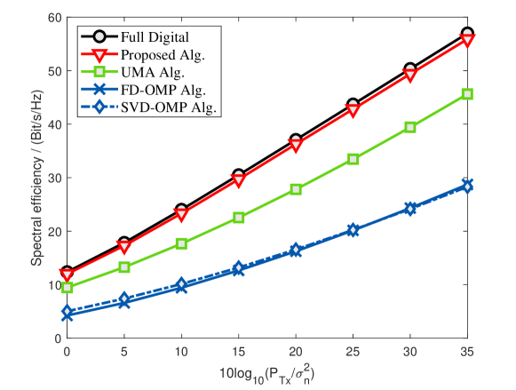
Figure 1: Comparison of spectral efficiency for the four linear hybrid transceiver designs and the full digital design based on capacity maximization. The mmWave channel with $N_{\rm path}=10$ paths is used in the simulation.

Initially, we assume that there is no channel estimation error for hybrid transceiver designs, and the results obtained are presented in Subsections VII-A and VII-B. However, we also consider the case where the channel estimation error is not negligible in Subsection VII-C.

VII-A MmWave Channel Case

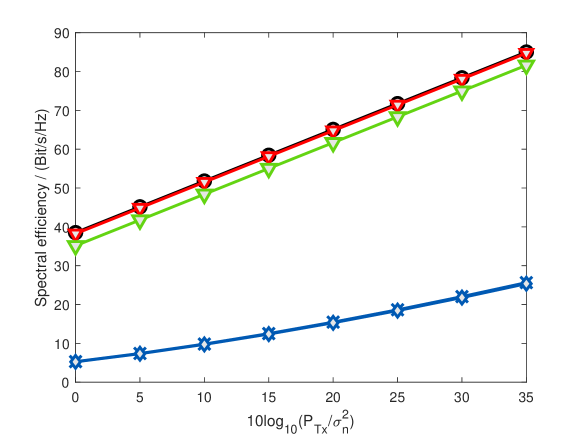
Figure 2: Comparison of spectral efficiency for the four linear hybrid transceiver designs and the full digital design based on capacity maximization. The mmWave channel with $N_{\rm path}=10$ paths is used in the simulation.

Fig. 1 compares the spectral efficiency performance of the four designs under the mmWave channel environment. Observe from Fig. 1 that the performance of our proposed robust hybrid transceiver design is very close to the optimal performance of the full digital design, which is significantly better than the other four hybrid transceiver designs. It is worth noting that the performance of the both OMP Algorithms are equally poor for this three-hop AF relay MIMO system with $N_{\rm RF}\!=\!N$. This is contrast to the traditional point-to-point MIMO systems, where the original OMP algorithm performs well [15, 35]. The results of Fig. 1 therefore show that the hybrid transceiver design based on the OMP Algorithm is not suitable for complicated multi-hop communication systems. As expected, the simulation results indicate that our proposed lower-complexity UMA Alg. suffers observable performance loss compared to our Proposed Alg. but crucially, it significantly outperforms the two OMP Algorithms. This indicates that if the low complexity is a critical performance measure, our UMA Alg. offers a suitable design choice.

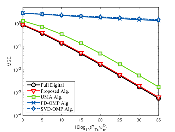
Figure 3: Comparison of transmitted signal MSE for the four linear hybrid transceiver designs and the full digital design based on MSE minimization. The mmWave channel with $N_{\rm path}=10$ paths is used in the simulation.

Further, in Fig. 2, the comparison of the spectral efficiency of the five designs in the massive MIMO communications is presented. MmWave channel is utilized in the simulation. The source, two relay nodes, and the destination are all equipped with $256$ antennas. From Fig. 2, it can be seen that the performance of the proposed algorithm outperforms the other four hybrid transceiver designs, which is nearly the same with the full digital transceiver. It is also shown in Fig. 2 that the sum rate of the UMA Alg. is quite close to that of the full digital design. This is because the extra antennas provide more spatial diversity and multiplexing gain for the hybrid transceivers. In addition, the spectral efficiency of the two OMP algorithms improves as well, but still falls largely behind of the proposed hybrid design. Therefore, the result indicates that the proposed algorithm retains its superiority in the channel scenario with 256 antennas, and it also shows the capability of the proposed hybrid design in massive MIMO channels.

Fig. 3 compares the MSE minimization performance of the five designs under the mmWave channel senario. The results obtained again demonstrate that the achievable performance of our robust hybrid transceiver design is very close to the powerful full digital design, namely, it is near optimal, while imposing substantially lower hardware costs in comparison with the optimal full digital design. The results of Figs. 3 also show that hybrid transceiver design based on the two OMP Algorithms are similarly very poor, and this indicates that the OMP based design is not suitable for multi-hop AF MIMO relaying networks under the MSE minimization criterion too. Observe that our UMA Alg. is capable of achieving considerably lower computational complexity by trading off some achievable MSE performance, compared with our near optimal robust hybrid transceiver design. In particular, it outperforms the OMP based design considerably.

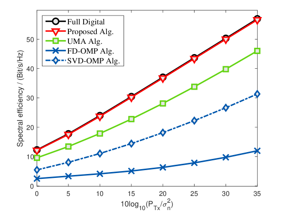
Figure 4: Comparison of spectral efficiency for the four linear hybrid transceiver designs and the full digital design based on capacity maximization. The mmWave channel with $N_{\rm path}=10$ paths is used in the simulation, and the number of RF-chains in each node is set to $N_{\rm RF}=6$.

In addition, the communication scenario with extra RF-chains is tested in Fig. 4. Specifically, in the simulation, the number of data streams remains $N\!=\!4$, and we set the number of RF-chains to $N_{\rm RF}\!=\!6$, which means there are 2 extra RF-chains that can be used to enhance the system performance. By comparing Fig. 4 with Fig. 1, it can be seen that with more RF-chains than data streams, the hybrid transceiver system performance can indeed be improved. In particular, from Fig. 4, it is clear that the performance of the Proposed Alg. is almost identical to that of the optimal full digital design, and the performance of the UMA Alg. is also improved slightly. Furthermore, the performance of the SVD-OMP Alg. is also improved, but it remains significantly worst than our low-complexity UMA Alg. design. However, for the FD-OMP Alg., increasing $N_{\rm RF}$ to more than $N$ actually degrades the system performance considerably. The reason is as follows. The need of $\bm{R}_{\bm{x}_{k}}$ in the FD-OMP Alg., required by the input full digital solution, naturally leads to mismatch between the optimal full digital transceiver and the FD-OMP Alg. based transceiver. The extra RF chains will magnify this mismatch, and results in a worse performance.

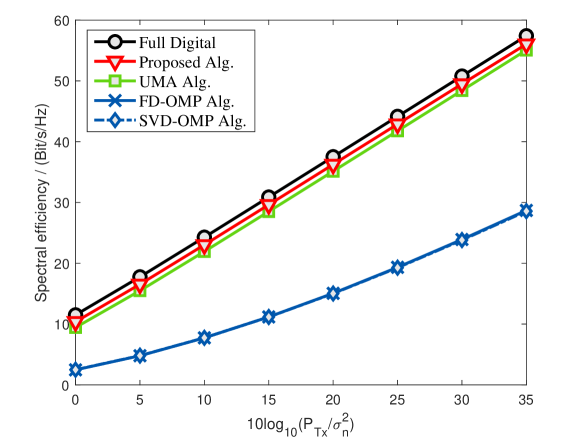
Figure 5: Comparison of spectral efficiency for the four linear hybrid transceiver designs and the full digital design based on capacity maximization. The RF Rayleigh channel is used in the simulation.

VII-B RF Channel Case

The simulation results for the RF Rayleigh channel are depicted in Fig. 5. It can be seen that under the RF Rayleigh channel environment, our robust hybrid transceiver design only suffers from very slight performance degradation, in comparison to the optimal full digital design. Furthermore, our low-complexity UMA Alg. now attains a performance close to that of the Proposed Alg., since the rich scatters in the RF channel environment provide much more tolerance to mismatch between the theoretical optimal analog beamformer and the actual analog beamformer. It is worth pointing out again that the two OMP Algorithms have a design challenge for Rayleigh channels, owing to the lack of steering vector based codebooks. Therefore, similar to [27], we have to use the phase matrix of the Rayleigh channel as the OMP codebook.

VII-C Robust Design with Channel Estimation Error

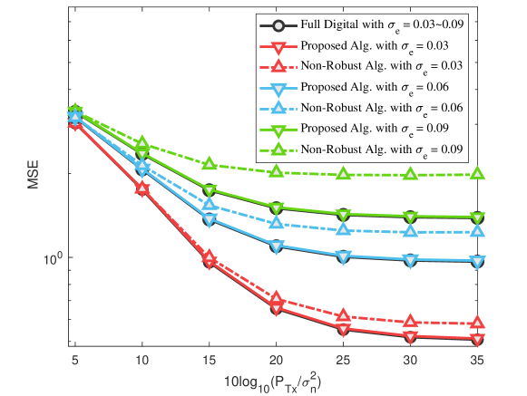
Figure 6: Comparison of transmitted signal MSE under different channel estimation errors for the proposed robust hybrid transceiver design, the full digital robust transceiver design, and non-robust hybrid transceiver design based on MSE maximization with $\alpha_{e}=0.6$. The RF Rayleigh channel is used in the simulation.

In the above simulation investigation, there exists no channel estimation error in hybrid transceiver designs. In practice, however, the channel estimation error always exists and cannot be neglected. Thus, the channel estimation error is considered. Specifically, the transmit correlation matrix of the channel error is defined based on the exponential model with the $i$th-row and $l$th-column element of the correlation matrix $\bm{\Psi}_{k}$ given by

$$[\bm{\Psi}_{k}]_{i,l}= \sigma_{e,k}\alpha_{e,k}^{\lvert i-l\rvert}.$$ (168)

Without loss of generality, it is assumed that the correlation coefficients $\{\sigma_{e,k}\}$ and the variances $\{\alpha_{e,k}\}$ of the transmit correlation matrix of channel error are the same for every channel, and they are denoted by $\sigma_{e}$ and $\alpha_{e}$, respectively. In the simulation, $\alpha_{e}=0.6$ is adopted. We consider our robust hybrid transceiver design, Proposed Alg., under this imperfect channel condition. Additionally, the counterpart of our Proposed Alg., which treats the estimated but inaccurate channel as the perfect one [7], is used for comparison, and it is denoted as Non-Robust Alg.

Only the RF Rayleigh channel senario is considered. Fig. 6 compares the performance of the proposed robust hybrid transceiver design, the full digital robust transceiver design [6] and non-robust hybrid transceiver design [7], in terms of MSE, under different channel estimation errors. From Fig. 6, it can be seen that the proposed robust hybrid transceiver design is very close to that of the optimal full digital robust transceiver design, and it achieves better performance than the non-robust hybrid transceiver design. Moreover, as the channel estimation error, i.e., $\sigma_{e}$, increases, the performance gap between our proposed robust hybrid transceiver design and the non-robust hybrid transceiver design becomes larger.

VIII Conclusions

In this paper, we have investigated robust hybrid transceiver optimization for multi-hop AF MIMO relaying networks, in which all nodes employ hybrid transceivers and multiple data streams are transmitted from source node simultaneously. A unified design framework has been proposed for both hybrid linear and nonlinear transceivers under generic objective functions, which also takes into account channel estimation error. Based on the proposed framework, it has been shown that the analog transceivers and digital transceivers can be decoupled without loss of optimality. Using matrix-monotonic optimization framework, the optimal structures of the analog and digital transceiver designs have been derived, which greatly simplify the hybrid transceiver optimizations. Based on the derived optimal structures, both analog precoders and combiners as well as digital forward matrices can be optimized separately and efficiently. Simulation results obtained have demonstrated that our proposed robust hybrid transceiver design only suffers from a very slight performance loss compared to the powerful full digital design. This confirms that our hybrid transceiver design attains near optimal performance, while imposing substantially lower hardware cost than the full digital design.

References

• [1] M. J. Farooq, H. ElSawy, and M.-S. Alouini, “A stochastic geometry model for multi-hop highway vehicular communication,” IEEE Trans. Wireless Commun., vol. 15, no. 3, pp. 2276–2291, 2016.
• [2] N. I. Miridakis, D. D. Vergados, and A. Michalas, “Dual-hop communication over a satellite relay and shadowed rician channels,” IEEE Trans. Veh. Technol., vol. 64, no. 9, pp. 4031–4040, 2015.
• [3] F. Ono, H. Ochiai, and R. Miura, “A wireless relay network based on unmanned aircraft system with rate optimization,” IEEE Trans. Wireless Commun., vol. 15, no. 11, pp. 7699–7708, 2016.
• [4] M. R. Khandaker and Y. Rong, “Transceiver optimization for multi-hop MIMO relay multicasting from multiple sources,” IEEE Trans. Wireless Commun., vol. 13, no. 9, pp. 5162–5172, Sep. 2014.
• [5] M. Mondelli, Q. Zhou, V. Lottici, and X. Ma, “Joint power allocation and path selection for multi-hop noncoherent decode and forward UWB communications,” IEEE Trans. Wireless Commun., vol. 13, no. 3, pp. 1397–1409, 2014.
• [6] C. Xing, S. Ma, Z. Fei, Y.-C. Wu, and H. V. Poor, “A general robust linear transceiver design for multi-hop amplify-and-forward MIMO relaying systems,” IEEE Trans. Signal Process., vol. 61, no. 5, pp. 1196–1209, 2013.
• [7] C. Xing, F. Gao, and Y. Zhou, “A framework for transceiver designs for multi-hop communications with covariance shaping constraints,” IEEE Trans. Signal Process., vol. 63, no. 15, pp. 3930–3945, Feb. 2015.
• [8] C. Xing, Y. Ma, Y. Zhou, and F. Gao, “Transceiver optimization for multi-hop communications with per-antenna power constraints.” IEEE Trans. Signal Process., vol. 64, no. 6, pp. 1519–1534, Jan. 2016.
• [9] M. Peng, Q. Hu, X. Xie, Z. Zhao, and H. V. Poor, “Network coded multihop wireless communication networks: Channel estimation and training design,” IEEE J. Sel. Areas Commun., vol. 33, no. 2, pp. 281–294, 2015.
• [10] D. Feng, C. Jiang, G. Lim, L. J. Cimini, G. Feng, and G. Y. Li, “A survey of energy-efficient wireless communications,” IEEE Commun. Surveys Tuts., vol. 15, no. 1, pp. 167–178, 2013.
• [11] S. Han, I. Chih-Lin, Z. Xu, and C. Rowell, “Large-scale antenna systems with hybrid analog and digital beamforming for millimeter wave 5G,” IEEE Commun. Mag., vol. 53, no. 1, pp. 186–194, 2015.
• [12] X. Zhang, A. F. Molisch, and S.-Y. Kung, “Variable-phase-shift-based RF-baseband codesign for MIMO antenna selection,” IEEE Trans. Signal Process., vol. 53, no. 11, pp. 4091–4103, 2005.
• [13] S. Kutty and D. Sen, “Beamforming for millimeter wave communications: An inclusive survey,” IEEE Commun. Surveys Tuts., vol. 18, no. 2, pp. 949–973, 2016.
• [14] T. E. Bogale, L. B. Le, A. Haghighat, and L. Vandendorpe, “On the number of RF chains and phase shifters, and scheduling design with hybrid analog-digital beamforming,” IEEE Trans. Wireless Commun., vol. 15, no. 5, pp. 3311–3326, 2016.
• [15] O. El Ayach, S. Rajagopal, S. Abu-Surra, Z. Pi, and R. W. Heath, “Spatially sparse precoding in millimeter wave MIMO systems,” IEEE Trans. Wireless Commun., vol. 13, no. 3, pp. 1499–1513, Mar. 2014.
• [16] W. Ni, X. Dong, and W.-S. Lu, “Near-optimal hybrid processing for massive MIMO systems via matrix decomposition,” IEEE Trans. Signal Process., vol. 65, no. 15, pp. 3922–3933, Aug. 2017.
• [17] D. Zhang, Y. Wang, X. Li, and W. Xiang, “Hybridly connected structure for hybrid beamforming in mmwave massive MIMO systems,” IEEE Trans. Commun., vol. 66, no. 2, pp. 662–674, 2018.
• [18] C. Lin, G. Y. Li, and L. Wang, “Subarray-based coordinated beamforming training for mmwave and sub-THz communications,” IEEE J. Sel. Areas Commun., vol. 35, no. 9, pp. 2115–2126, 2017.
• [19] F. Sohrabi and W. Yu, “Hybrid digital and analog beamforming design for large-scale antenna arrays,” IEEE J. Sel. Topics Signal Process., vol. 10, no. 3, pp. 501–513, Apr. 2016.
• [20] X. Yu, J.-C. Shen, J. Zhang, and K. B. Letaief, “Alternating minimization algorithms for hybrid precoding in millimeter wave MIMO systems,” IEEE J. Sel. Topics Signal Process., vol. 10, no. 3, pp. 485–500, Feb. 2016.
• [21] T. Lin, J. Cong, Y. Zhu, J. Zhang, and K. B. Letaief, “Hybrid beamforming for millimeter wave systems using the MMSE criterion,” IEEE Trans. Commun., vol. 67, no. 5, pp. 3693–3708, May 2019.
• [22] S. S. Ioushua and Y. C. Eldar, “A family of hybrid analog–digital beamforming methods for massive MIMO systems,” IEEE Trans. Signal Process., vol. 67, no. 12, pp. 3243–3257, May 2019.
• [23] V. V. Ratnam, A. F. Molisch, O. Y. Bursalioglu, and H. C. Papadopoulos, “Hybrid beamforming with selection for multiuser massive MIMO systems,” IEEE Trans. Signal Process., vol. 66, no. 15, pp. 4105–4120, Aug. 2018.
• [24] A. Alkhateeb, G. Leus, and R. W. Heath, “Limited feedback hybrid precoding for multi-user millimeter wave systems,” IEEE Trans. Wireless Commun., vol. 14, no. 11, pp. 6481–6494, 2015.
• [25] J. Li, L. Xiao, X. Xu, and S. Zhou, “Robust and low complexity hybrid beamforming for uplink multiuser mmwave MIMO systems,” IEEE Commun. Lett., vol. 20, no. 6, pp. 1140–1143, 2016.
• [26] R. Mai and T. Le-Ngoc, “Nonlinear hybrid precoding for coordinated multi-cell massive MIMO systems,” IEEE Trans. Veh. Technol., vol. 68, no. 3, pp. 2459–2471, Mar. 2019.
• [27] C. Xing, X. Zhao, W. Xu, X. Dong, and G. Y. Li, “A framework on hybrid MIMO transceiver design based on matrix-monotonic optimization,” IEEE Trans. Signal Process., vol. 67, no. 13, pp. 3531–3546, Apr. 2019.
• [28] Q. Shi and M. Hong, “Spectral efficiency optimization for millimeter wave multiuser MIMO systems,” IEEE J. Sel. Topics Signal Process., vol. 12, no. 3, pp. 455–468, Jun. 2018.
• [29] L. Zhao, D. W. K. Ng, and J. Yuan, “Multi-user precoding and channel estimation for hybrid millimeter wave systems,” IEEE J. Sel. Areas Commun., vol. 35, no. 7, pp. 1576–1590, 2017.
• [30] Z. Li, S. Han, and A. F. Molisch, “Optimizing channel-statistics-based analog beamforming for millimeter-wave multi-user massive MIMO downlink,” IEEE Trans. Wireless Commun., vol. 16, no. 7, pp. 4288–4303, 2017.
• [31] P. Raviteja, Y. Hong, and E. Viterbo, “Millimeter wave analog beamforming with low resolution phase shifters for multiuser uplink,” IEEE Trans. Veh. Technol., vol. 67, no. 4, pp. 3205–3215, Dec. 2017.
• [32] J. Du, W. Xu, H. Shen, X. Dong, and C. Zhao, “Hybrid precoding architecture for massive multiuser MIMO with dissipation: Sub-connected or fully connected structures?” IEEE Trans. Wireless Commun., vol. 17, no. 8, pp. 5465–5479, Aug. 2018.
• [33] S. Gong, C. Xing, V. K. N. Lau, S. Chen, and L. Hanzo, “Majorization-minimization aided hybrid transceivers for MIMO interference channels,” arXiv:1911.05906 [cs.IT], Nov. 2019.
• [34] S. Sun, T. S. Rappaport, M. Shafi, and H. Tataria, “Analytical framework of hybrid beamforming in multi-cell millimeter-wave systems,” IEEE Trans. Wireless Commun., vol. 17, no. 11, pp. 7528–7543, Nov. 2018.
• [35] J. Lee and Y. H. Lee, “AF relaying for millimeter wave communication systems with hybrid RF/baseband MIMO processing,” in Proc. IEEE Int. Conf. Commun., Jun. 2014, pp. 5838–5842.
• [36] W. Xu, J. Liu, S. Jin, and X. Dong, “Spectral and energy efficiency of multi-pair massive MIMO relay network with hybrid processing,” IEEE Trans. Commun., vol. 65, no. 9, pp. 3794–3809, 2017.
• [37] X. Xue, Y. Wang, L. Dai, and C. Masouros, “Relay hybrid precoding design in millimeter-wave massive MIMO systems,” IEEE Trans. Signal Process., vol. 66, no. 8, pp. 2011–2026, 2018.
• [38] Y. Cai, Y. Xu, Q. Shi, B. Champagne, and L. Hanzo, “Robust joint hybrid transceiver design for millimeter wave full-duplex mimo relay systems,” IEEE Trans. Wireless Commun., vol. 18, no. 2, pp. 1199–1215, Feb. 2019.
• [39] C. Xing, S. Ma, and Y. Zhou, “Matrix-monotonic optimization for MIMO systems,” IEEE Trans. Signal Process., vol. 63, no. 2, pp. 334–348, Jan. 2015.
• [40] C. Xing, S. Li, Z. Fei, and J. Kuang, “How to understand linear minimum mean-square-error transceiver design for multiple-input–multiple-output systems from quadratic matrix programming,” IET Commun., vol. 7, no. 12, pp. 1231–1242, 2013.
• [41] R. F. Fischer, Precoding and signal shaping for digital transmission. John Wiley & Sons, 2005.
• [42] C. Xing, M. Xia, F. Gao, and Y.-C. Wu, “Robust transceiver with Tomlinson-Harashima precoding for amplify-and-forward MIMO relaying systems,” IEEE J. Sel. Areas Commun., vol. 30, no. 8, pp. 1370–1382, Sep. 2012.
• [43] R. López-Valcarce, “Realizable linear and decision feedback equalizers: properties and connections,” IEEE Trans. Signal Process., vol. 52, no. 3, pp. 757–773, 2004.
• [44] C. Xing, Y. Jing, and Y. Zhou, “On weighted MSE model for MIMO transceiver optimization,” IEEE Trans. Veh. Technol., vol. 66, no. 8, pp. 7072–7085, 2017.
• [45] D. P. Palomar and Y. Jiang, MIMO Transceiver Design via Majorization Theory. Now Foundations and Trends, 2007.
• [46] E. Jorswieck and H. Boche, Majorization and Matrix Monotone Functions in Wireless Communications. Now Foundations and Trends, 2007.
• [47] A. W. Marshall, I. Olkin, and B. C. Arnold, Inequalities: Theory of majorization and its applications. Springer-Verlag New York, 2011.
• [48] G. H. Golub and C. F. Van Loan, Matrix computations. Johns Hopkins University Press, 2012, vol. 3.