Quantifying Dynamic Leakage
Complexity Analysis and Model Counting-based Calculation

Abstract

A program is non-interferent if it leaks no secret information to an observable output. However, non-interference is too strict in many practical cases and quantitative information flow (QIF) has been proposed and studied in depth. Originally, QIF is defined as the average of leakage amount of secret information over all executions of a program. However, a vulnerable program that has executions leaking the whole secret but has the small average leakage could be considered as secure. This counter-intuition raises a need for a new definition of information leakage of a particular run, i.e., dynamic leakage. As discussed in [5], entropy-based definitions do not work well for quantifying information leakage dynamically; Belief-based definition on the other hand is appropriate for deterministic programs, however, it is not appropriate for probabilistic ones.

In this paper, we propose new simple notions of dynamic leakage based on entropy which are compatible with existing QIF definitions for deterministic programs, and yet reasonable for probabilistic programs in the sense of [5]. We also investigated the complexity of computing the proposed dynamic leakage for three classes of Boolean programs. We also implemented a tool for QIF calculation using model counting tools for Boolean formulae. Experimental results on popular benchmarks of QIF research show the flexibility of our framework. Finally, we discuss the improvement of performance and scalability of the proposed method as well as an extension to more general cases.

1 Introduction

Researchers have realized the importance of knowing where confidential information reaches by the execution of a program to verify whether the program is safe. The non-interference property, namely, any change of confidential input does not affect public output, was coined in 1982 by Goguen and Meseguer [14] as a criterion for the safety. This property, however, is too strict in many practical cases, such as password verification, voting protocol and averaging scores. A more elaborated notion called quantitative information flow (QIF) [23] has been getting much attention of the community. QIF is defined as the amount of information leakage from secret input to observable output. The program can be considered to be safe (resp. vulnerable) if this quantity is negligible (resp. large). QIF analysis is not easier than verifying non-interference property because if we can calculate QIF of a program, we can decide whether it satisfies non-interference or not. QIF calculation is normally approached in an information-theoretic fashion to consider a program as a communication channel with input as source, and output as destination. The quantification is based on entropy notions including Shannon entropy, min-entropy and guessing entropy [23]. QIF (or the information leakage) is defined as the remaining uncertainty about secret input after observing public output, i.e., the mutual information between source and destination of the channel. Another quantification proposed by Clarkson, et al. [11], is the difference between ‘distances’ (Kullback-Leibler divergence) from the probability distribution on secret input that an attacker believes in to the real distribution, before and after observing the output values.
While QIF is about the average amount of leaked information over all observable outputs, dynamic leakage is about the amount of information leaked by observing a particular output. Hence, QIF is aimed to verify the safety of a program in a static scenario in compile time, and dynamic leakage is aimed to verify the safety of a specific running of a program. So which of them should be used as a metric to evaluate a system depends on in what scenario the software is being considered.

Example 1

if $source<16$ then $output\leftarrow 8+source$
else $output\leftarrow 8$

In Example 1 above, assume $source$ to be a positive integer, then there are 16 possible values of $output$, from 8 to 23. While an observable value between 9 and 23 reveals everything about the secret variable, i.e., there is only one possible value of $source$ to produce such $output$, a value of 8 gives almost nothing, i.e., there are so many possible values of $source$ which produce 8 as output. Taking the average of leakages on all possible execution paths results in a relatively small value, which misleads us into regarding that the vulnerability of this program is small. Therefore, it is crucial to differentiate risky execution paths from safe ones by calculating dynamic leakage, i.e., the amount of information can be learned from observing the output which is produced by a specific execution path. But, as discussed in [5], any of existing QIF models (either entropy based or belief tracking based) does not always seem reasonable to quantify dynamic leakage. For example, entropy-based measures give sometimes negative leakage. Usually, we consider that the larger the value of the measure is, the more information is leaked, and in particular, no information is leaked when the value is 0. In the interpretation, it is not clear how we should interpret a negative value as a leakage metric. Actually, [5] claims that the non-negativeness is a requirement for a measure of dynamic QIF. Also, MONO, one of the axioms for QIF in [2] turns out to be identical to this non-negative requirement. Belief-based one always give non-negative leakage for deterministic programs but it may become negative for probabilistic programs. In addition, the measure using belief model depends on secret values. This would imply (1) even if a same output value is observed, the QIF may become different depending on which value is assumed to be secret, which is unnatural, and (2) a side-channel may exist when further processing is added by system managers after getting quantification result. Hence, as suggested in [5], it is better to introduce a new notion for quantifying dynamic leakage caused by observing a specific output value.
The contributions of this paper are three-fold.

• We present our criteria for an appropriate definition of dynamic leakage and propose two notions that satisfy those criteria. We propose two notions because there is a trade-off between the easiness of calculation and the preciseness (see Section 2).

• Complexity of computing the proposed dynamic leakages is analyzed for three classes of Boolean programs.

• By applying model counting of logical formulae, a prototype was implemented and feasibility of computing those leakages is discussed based on experimental results.

According to [5], we arrange three criteria that a ‘good’ definition of dynamic leakage should satisfy, namely, the measure should be (R1) non-negative, (R2) independent of a secret value to prevent a side channel and (R3) compatible with existing notions to keep the consistency within QIF as a whole (both dynamic leakage and normal QIF). Based on those criteria, we come up with two notions of dynamic leakage QIF1 and QIF2, where both of them satisfy all (R1), (R2) and (R3). QIF1, motivated by entropy-based approach, takes the difference between the initial and remaining self-information of the secret before and after observing output as dynamic leakage. On the other hand, QIF2 models that of the joint probability between secret and output. Because both of them are useful in different scenarios, we studied these two models in parallel in the theoretical part of the paper. We call the problems of computing QIF1 and QIF2 for Boolean programs CompQIF1 and CompQIF2, respectively. For example, we show that even for deterministic loop-free programs with uniformly distributed input, both CompQIF1 and CompQIF2 are $\sharp P$-hard. Next, we assume that secret inputs of a program are uniformly distributed and consider the following method of computing QIF1 and QIF2 (only for deterministic programs for QIF2 by the technical reason mentioned in Section 4): (1) translate a program into a Boolean formula that represents relationship among values of variables during a program execution, (2) augment additional constraints that assign observed output values to the corresponding variables in the formula, (3) count models of the augmented Boolean formula projected on secret variables, and (4) calculate the necessary probability and dynamic leakage using the counting result. Based on this method, we conducted experiments using our prototype tool with benchmarks taken from QIF related literatures, in which programs are deterministic, to examine the feasibility of automatic calculation. We also give discussion, in subsection 5.3, on difficulties and possibilities to deal with more general cases, such as, of probabilistic programs. In step (3), we can flexibly use any off-the-shelf model counter. To investigate the scalability of this method, we used four state-of-the-art counters, SharpCDCL [15] and GPMC [24, 32] for SAT-based counting, an improved version of aZ3 [22] for SMT-based counting, and DSharp-p [20, 30] for SAT-based counting in d-DNNF fashion. Finally, we discuss the feasibility of automatic calculation of the leakage in general case.

Related work The very early work on computational complexity of QIF is that of Yasuoka and Terauchi. They proved that even the problem of comparing QIF of two programs, which is obviously not more difficult than calculating QIF, is not a $k$-safety property for any $k$ [27]. Consequently, self-composition, a successful technique to verify non-interference property, is not applicable to the comparison problem. Their subsequent work [28] proves a similar result for bounding QIF, as well as the $PP$-hardness of precisely quantifying QIF in all entropy-based definitions for loop-free Boolean programs. Chadha and Ummels [9] show that the QIF bounding problem of recursive programs is not harder than checking reachability for those programs. Despite given those evidences about the hardness of calculating QIF, for this decade, precise QIF analysis gathers much attention of the researchers. In [15], Klebanov et al. reduce QIF calculation to $\sharp$SAT problem projected on a specific set of variables as a very first attempt to tackle with automating QIF calculation. On the other hand, Phan et al. reduce QIF calculation to $\sharp$SMT problem for utilizing existing SMT (satisfiability modulo theory) solver. Recently, Val et al. [25] reported a method that can scale to programs of 10,000 lines of code but still based on SAT solver and symbolic execution. However, there is still a gap between such improvements and practical use, and researchers also work on approximating QIF. Köpf and Rybalchenko [16] propose approximated QIF computation by sandwiching the precise QIF by lower and upper bounds using randomization and abstraction, respectively with a provable confidence. LeakWatch of Chothia et al. [10], also give approximation with provable confidence by executing a program multiple times. Its descendant called HyLeak [7] combines the randomization strategy of its ancestor with precise analysis. Also using randomization but in Markov Chain Monte Carlo (MCMC) manner, Biondi et al. [6] utilize ApproxMC2, an existing model counter created by some of the co-authors. ApproxMC2 provides approximation on the number of models of a Boolean formula in CNF with adjustable precision and confidence. ApproxMC2 uses hashing technique to divide the solution space into smaller buckets with almost equal number of elements, then count the models for only one bucket and multiply it by the number of buckets. As for dynamic leakage, McCamant et al. [17] consider QIF as network flow through programs and propose a dynamic analysis method that can work with executable files. Though this model can scale to very large programs, its precision is relatively not high. Alvim et al. [2] give some axioms for a reasonable definition of QIF to satisfy and discuss whether some definitions of QIF satisfy the axioms. Note that these axioms are for static QIF measures, which differ from dynamic leakage. However, given a similarity between static and dynamic notions, we investigated how our new dynamic notions fit in the lens of the axioms (refer to Section 2).

Dynamic information flow analysis (or taint analysis) is a bit confusing term that does not mean an analysis of dynamic leakage, but a runtime analysis of information flow. Dynamic analysis can abort a program as soon as an unsafe information flow is detected. Also, hybrid analysis has been proposed for improving dynamic analysis that may abort a program too early or unnecessarily. In hybrid analysis, the unexecuted branches of a program is statically analyzed in parallel with the executed branch. Among them, Bielova et al. [4] define the knowledge $\kappa(z)$ of a program variable $z$ as the information on secret that can be inferred from $z$ (technically, $\kappa(z)^{-1}(v)$ is the same of the pre-image of an observed value $v$ of $z$, defined in Section 2). In words, hybrid analysis updates the ‘dynamic leakage’ under the assumption that the program may terminate at each moment. Our method is close to [4] in the sense that the knowledge $\kappa(z)^{-1}(v)$ is computed. The difference is that we conduct the analysis after the a program is terminated and $v$ is given. We think this is not a disadvantage compared with hybrid analysis because the amount of dynamic leakage of a program is not determined until a program terminates in general.

Structure of the remaining parts: Section 2 is dedicated to introduce new notions, i.e., QIF1 and QIF2, of dynamic leakage and some properties of them. The computational complexity of CompQIF1 and CompQIF2 is discussed in Section 3. Section 4 gives details on calculating dynamic leakage based on model counting. Experimental results and discussion are provided in Section 5 and the paper is concluded in Section 6.

2 New Notions for Dynamic Leakage

The standard notion for static quantitative information flow (QIF) is defined as the mutual information between random variables $S$ for secret input and $O$ for observable output:

$$\mbox{QIF}=H(S)-H(S|O)$$ (1)

where $H(S)$ is the entropy of $S$ and $H(S|O)$ is the expected value of $H(S|o)$, which is the conditional entropy of $S$ when observing an output $o$. Shannon entropy and min-entropy are often used as the definition of entropy, and in either case, $H(S)-H(S|O)\geq 0$ always holds by the definition.

In [5], the author discusses the appropriateness of the existing measures for dynamic QIF and points out their drawbacks, especially, each of these measures may become negative. Hereafter, let ${\cal S}$ and ${\cal O}$ denote the finite sets of input values and output values, respectively. Since $H(S|O)=\sum_{o\in{\cal O}}p(o)H(S|o)$, [5] assumes the following measure obtained by replacing $H(S|O)$ with $H(S|o)$ in (1) for dynamic QIF:

$$\mbox{QIF}^{dyn}(o)=H(S)-H(S|o).$$ (2)

However, $\mbox{QIF}^{dyn}(o)$ may become negative even if a program is deterministic (see Example 2). Another definition of dynamic QIF is proposed in [11] as

$$\mbox{QIF}^{belief}(\dot{s},o)=D_{KL}(p_{\dot{s}}||p_{S})-D_{KL}(p_{\dot{s}}||p_{S|o})$$ (3)

where $D_{KL}$ is KL-divergence defined as $D_{KL}(p||q)=\sum_{s\in{\cal S}}p(s)\log\frac{p(s)}{q(s)}$, and $p_{\dot{s}}(s)=1$ if $s=\dot{s}$ and $p_{\dot{s}}(s)=0$ otherwise. Intuitively, $\mbox{QIF}^{belief}(\dot{s},o)$ represents how closer the belief of an attacker approaches to the secret $\dot{s}$ by observing $o$. For deterministic programs, $\mbox{QIF}^{belief}(\dot{s},o)=-\log p(o)\geq 0$ [5]. However, $\mbox{QIF}^{belief}$ may still become negative if a program is probabilistic (see Example 3).

Let $P$ be a program with secret input variable $S$ and observable output variable $O$. For notational convenience, we identify the names of program variables with the corresponding random variables. Throughout the paper, we assume that a program always terminates. The syntax and semantics of programs assumed in this paper will be given in the next section. For $s\in{\cal S}$ and $o\in{\cal O}$, let $p_{SO}(s,o)$, $p_{O|S}(o|s)$, $p_{S|O}(s|o)$, $p_{S}(s)$, $p_{O}(o)$ denote the joint probability of $s\in{\cal S}$ and $o\in{\cal O}$, the conditional probability of $o\in{\cal O}$ given $s\in{\cal S}$ (the likelihood), the conditional probability of $s\in{\cal S}$ given $o\in{\cal O}$ (the posterior probability), the marginal probability of $s\in{\cal S}$ (the prior probability) and the marginal probability of $o\in{\cal O}$, respectively. We often omit the subscripts as $p(s,o)$ and $p(o|s)$ if they are clear from the context. By definition,

$$p(s,o) = p(s|o)p(o)=p(o|s)p(s),$$ (4)

$$p(o) = \sum_{s\in{\cal S}}p(s,o),$$ (5)

$$p(s) = \sum_{o\in{\cal O}}p(s,o).$$ (6)

We assume that (the source code of) $P$ and the prior probability $p(s)$ ($s\in{\cal S}$) are known to an attacker. For $o\in{\cal O}$, let $\mbox{pre}_{P}(o)=\{s\in{\cal S}\mid p(s|o)>0\}$, which is called the pre-image of $o$ (by the program $P$).

Considering the discussions in the literature, we aim to define new notions for dynamic QIF that satisfy the following requirements:

1. Dynamic QIF should be always non-negative because an attacker obtains some information (although sometimes very small or even zero) when he observes an output of the program.

2. It is desirable that dynamic QIF is independent of a secret input $s\in{\cal S}$. Otherwise, the controller of the system may change the behavior for protection based on the estimated amount of the leakage that depends on $s$, which may be a side channel for an attacker.

3. The new notion should be compatible with the existing notions when we restrict ourselves to special cases such as deterministic programs, uniformly distributed inputs, and taking the expected value.

The first proposed notion is the self-information of the secret inputs consistent with an observed output $o\in{\cal O}$. Equivalently, the attacker can narrow down the possible secret inputs after observing $o$ to the pre-image of $o$ by the program. We consider the self-information of $s\in\mathcal{S}$ after the observation as the probability of $s$ divided by the sum of the probabilities of the inputs in the pre-image of $o$ (see the upper part of Fig. 1).

$$\mbox{QIF1}(o) = -\log(\sum_{s^{\prime}\in\mbox{pre}_{P}(o)}p(s^{\prime})).$$ (7)

The second notion is the self-information of the joint events $s^{\prime}\in{\cal S}$ and an observed output $o\in{\cal O}$ (see the lower part of Fig. 1). This is equal to the the self-information of $o$.

$$\mbox{QIF2}(o) = -\log(\sum_{s^{\prime}\in{\cal S}}p(s^{\prime},o))$$ (8)

$$=-\log p(o) = -\log p(s,o)+\log p(s|o).$$ (9)

Both notions are defined by considering how much possible secret input values are reduced by observing an output. We propose two notions because there is a trade-off between the easiness of calculation and the appropriateness. As illustrated in Example 3, QIF2 can represent the dynamic leakage more appropriately than QIF1 in some cases. On the other hand, the calculation of QIF1 is easier than QIF2 as discussed in Section 4. Both notions are independent of the secret input $s\in{\cal S}$ (Requirement (R2)).

$$0\leq\mbox{QIF1}(o)\leq\mbox{QIF2}(o).$$ (10)

If we assume Shannon entropy,

QIF $$= -\sum_{s\in{\cal S}}{p(s)\log p(s)}$$ (12)

$$\quad+\sum_{o\in{\cal O}}{p(o)\sum_{s\in{\cal S}}{p(s|o)\log p(s|o)}}$$

$$= -\sum_{s\in{\cal S}}{p(s)\log p(s)}$$

$$\quad+\sum_{s\in{\cal S},o\in{\cal O}}{p(s,o)\log p(s|o)}.$$

If a program is deterministic, for each $s\in{\cal S}$, there is exactly one $o_{s}\in{\cal O}$ such that $p(s,o_{s})=p(s)$ and $p(s,o)=0$ for $o\not=o_{s}$, and therefore

QIF $$= \sum_{s\in{\cal S},o\in{\cal O}}{p(s,o)(-\log p(s,o)+\log p(s|o))}.$$ (13)

Comparing (9) and (13), we see that QIF is the expected value of QIF2, which suggests the compatibility of QIF2 with QIF (Requirement (R3)) when a program is deterministic. Also, if a program is deterministic, $\mbox{QIF}^{belief}(\dot{s},o)=-\log p(o)$, which coincides with $\mbox{QIF2}(o)$ (Requirement (R3)). By (10), Requirement (R1) is satisfied. Also in (10), $\mbox{QIF1}(o)=\mbox{QIF2}(o)$ holds for every $o\in{\cal O}$ if and only if the program is deterministic.

Theorem 2.1

If a program $P$ is deterministic, for every $o\in{\cal O}$ and $s\in{\cal S}$,

$$\mbox{QIF}^{belief}(s,o)=\mbox{QIF1}(o)=\mbox{QIF2}(o)=-\log p(o).$$

If input values are uniformly distributed, $\mbox{QIF1}(o)=$ $\log\frac{|{\cal S}|}{|\mbox{pre}_{P}(o)|}$ for every $o\in{\cal O}$. ∎

Figure 1: QIF1 (the upper) and QIF2 (the lower)

Let us get back to the Example 1 in the previous section to see how new notions convey the intuitive meaning of dynamic leakage. We assume: both $source$ and $output$ are 8-bit numbers of which values are in $0..255$, $source$ is uniformly distributed over this range. Then, because the program in this example is deterministic, as mentioned above QIF1 coincides with QIF2. We have $\mbox{QIF1}(output=8)=-\log\frac{241}{256}=0.087bits$ while $\mbox{QIF1}(output=o)=-\log\frac{1}{256}=8bits$ for every $o$ between 9 and 23. This result addresses well the problem of failing to differentiate vulnerable output from safe ones of QIF.

Example 2

Consider the following program taken from Example 1 of [5]:

if $S=s_{1}$ then $O\leftarrow a$ else $O\leftarrow b$

Assume that the probabilities of inputs are $p(s_{1})=0.875$, $p(s_{2})=0.0625$ and $p(s_{3})=0.0625$. Then, we have the following output and posterior probabilities:

$p(a)=0.875,p(b)=0.125$
$p(s_{1}|a)=1,p(s_{2}|a)=p(s_{3}|a)=0$
$p(s_{1}|b)=0,p(s_{2}|b)=p(s_{3}|b)=0.5$

If we use Shannon entropy, $H(S)=0.67$, $H(S|a)=0$ and $H(S|b)=1$. Thus, $\mbox{QIF}^{dyn}(b)=-0.33$, which is negative as pointed out in [5]. Also, $\mbox{QIF2}(a)=-\log p(a)=-\log 0.875=0.19$ and $\mbox{QIF2}(b)=-\log p(b)=-\log 0.125=3$. $\mbox{QIF2}(a)<\mbox{QIF2}(b)$ reflects the fact that the difference of the posterior and the prior of each input when observing $b$ is larger ($s_{1}:0.875\to 0$, $s_{2},s_{3}:0.0625\to 0.5$) than observing $a$ ($s_{1}:0.875\to 1$, $s_{2},s_{3}:0.0625\to 0$).

Since the program is deterministic, $\mbox{QIF}^{belief}(s,o)=\mbox{QIF1}(o)=\mbox{QIF2}(o)$.

$$\begin{array}[]{c|cc}o&a&b\\ \hline\cr\mbox{QIF}^{dyn}(o)&0.67&-0.33\\ \mbox{QIF2}(o)&0.19&3\end{array}$$

∎

Example 3

The next program is quoted from Example 2 of [5] where $c_{1~{}r}[]_{1-r}~{}c_{2}$ means that the program chooses $c_{1}$ with probability $r$ and $c_{2}$ with probability $1-r$.

if $S=s_{1}$ then $O\leftarrow a~{}_{0.81}[]_{0.19}O\leftarrow b$
else $O\leftarrow a~{}_{0.09}[]_{0.91}O\leftarrow b$

Assume that the probabilities of inputs are $p(s_{1})=0.25$ and $p(s_{2})=0.75$. $(p(a),p(b))=(0.25,0.75)\begin{pmatrix}0.81&0.19\\ 0.09&0.91\end{pmatrix}=(0.27,0.73)$ and the posterior probabilities are calculated by (4) as:

$p(s_{1}|a)=0.75,p(s_{2}|a)=0.25$
$p(s_{1}|b)=0.065,p(s_{2}|b)=0.935$

Let us use Shannon entropy for $\mbox{QIF}^{dyn}$. As $H(S)=H(S|a)=-0.25\log 0.25-0.75\log 0.75$, $\mbox{QIF}^{dyn}(a)=H(S)-H(S|a)=0$. As already discussed in [5], $\mbox{QIF}^{dyn}(a)=0$ though an attacker may think that $S=s_{1}$ is more probable by observing $O=a$. For each $o\in\{a,b\}$, $\mbox{QIF}^{belief}(s,o)$ takes different values (one of them is negative) depending on whether $s=s_{1}$ or $s_{2}$ is the secret input. $\mbox{QIF2}(a)=-\log p(a)=-\log 0.27=1.89$ and $\mbox{QIF2}(b)=-\log p(b)=-\log 0.73=0.45$. $\mbox{QIF1}(a)=\mbox{QIF1}(b)=0$ because the set of possible input values does not shrink whichever $a$ or $b$ is observed. Similarly to Example 2, $\mbox{QIF2}(a)>\mbox{QIF2}(b)$ reflects the fact that the probability of each input when observing $a$ varies more largely ($s_{1}:0.25\to 0.75$, $s_{2}:0.75\to 0.25$) than when observing $b$ ($s_{1}:0.25\to 0.065$, $s_{2}:0.75\to 0.935$). In this example, the number $|{\cal S}|$ of input values is just two, but in general, $|{\cal S}|$ is larger and we can expect $|\mbox{pre}_{P}(o)|$ is much smaller than $|{\cal S}|$ and QIF1 serves a better measure for dynamic QIF.

$$\begin{array}[]{c|cc}o&a&b\\ \hline\cr\mbox{QIF}^{dyn}(o)&0&0.46\\ \mbox{QIF}^{belief}(s_{1},o)&1.58&-1.94\\ \mbox{QIF}^{belief}(s_{2},o)&-1.58&0.32\\ \mbox{QIF1}(o)&0&0\\ \mbox{QIF2}(o)&1.89&0.45\end{array}$$

A program is non-interferent if for every $o\in{\cal O}$ such that $p(o)>0$ and for every $s\in{\cal S}$, $p(o)=p(o|s)$. Assume a program $P$ is non-interferent. By (4), $p(s)=p(s|o)$ for every $o\in{\cal O}$ ($p(o)>0$) and $s\in{\cal S}$, then QIF = 0 by (12). If $P$ is deterministic in addition, $p(o)=p(o|s)=1$ for $o\in{\cal O}$ ($p(o)>0$) and $s\in{\cal S}$. That is, if a program is deterministic and non-interferent, it has exactly one possible output value.

Relationship to the hybrid monitor Let us see how our notions relate to the knowledge tracking hybrid monitor proposed by Bielova et al. [4].

Example 4

Consider the following program taken from Program 5 of [4]:

if $h$ then $z$ $\leftarrow$ $x$ + $y$
else $z$ $\leftarrow$ $y$ - $x$;
output $z$

where $h$ is a secret input, $x$ and $y$ are public inputs and $z$ is a public output.

In [4], the knowledge about secret input $h$ carried by public output $z$ is $\kappa(z)=\lambda\rho.$if$([\![h]\!]_{\rho},[\![x+y]\!]_{\rho},[\![y-x]\!]_{\rho})$ where $\rho$ is an initial environment (an assignment of values to $h$, $x$ and $y$) and $[\![e]\!]_{\rho}$ is the evaluation of $e$ in $\rho$. If $h=1$, $x=0$ and $y=1$, then $z=1$. In [4], to verify whether this value of $z$ reveals any information about $h$ in this setting of public inputs (i.e., $x=0$, $y=1$), they take $\kappa(z)^{-1}(1)=\{\rho|$if$([\![h]\!]_{\rho},[\![x+y]\!]_{\rho},[\![y-x]\!]_{\rho})=1\}=\{\rho|$if$([\![h]\!]_{\rho},1,1)=1\}$. Because if$([\![h]\!]_{\rho},1,1)=1$ for every $\rho$, [4] concluded that $z=1$ in that setting leaks no information.
On the other hand, with that settings of $x=0$ and $y=1$, given $z=1$ as the observed output, $h$ can be either $true$ or $false$. For the program is deterministic, $\mbox{QIF1}(z=1)=\mbox{QIF2}(z=1)=-\log\sum_{p(s^{\prime}|o)>0}p(s^{\prime})=-\log(p(h=true)+p(h=false))=-\log 1=0$, which is consistent with that of [4] though the approach looks different. Actually, the function $\kappa(z)$ encodes all information revealed from a value of $z$ about secret input. By applying $\kappa(z)^{-1}$ for a specific value $o$ of $z$, we get the pre-image of $o$. In other words, $\kappa(z)^{-1}(o)$ is exactly what we are getting toward quantifying our notions of dynamic leakage. The monitor proposed in [4] tracks the knowledge about secret input carried by all variables along an execution of a program according to the inlined operational semantics. It seems, however, impractical to store all the knowledge during an execution, and furthermore, it would take time to compute the inverse of the knowledge when an observed output is fixed.

The three requirements (R1), (R2) and (R3) we presented summarize the intuitions about dynamic leakage following the spirit of [5]. However, those requirements lack of a firm back-up theory, whilst in [2] Alvim et al. provide a set of axioms for QIF. Despite there is difference between QIF and dynamic leakage, we investigated how well our notions fit in the lens of those axioms to confirm their feasibility to be used as a metric. For the limitations of space, we will skip detailed explanation for the quite trivial results.
(1) For prior vulnerability, both QIF1 and QIF2 satisfy CONTINUITY, CONVEXITY (also the loosen version Q-CONVEXITY).
(2) For posterior vulnerability, exactly speaking, we cannot construct the channel matrix $C$, because dynamic leakage is about one specific output value but the matrix is for all possibilities. Hence, conceptually, those axioms are not applicable in this context. However, by capturing the intuitive interpretation of the axioms, we made a small modification (i.e., to use $\mathbb{D}\mathcal{Y}\rightarrow\mathbb{R}^{+}$ in stead of $\mathbb{D}^{2}\mathcal{X}\rightarrow\mathbb{R}^{+}$ as the type of posterior vulnerability) to investigate the new notions under the spirit of axioms. So, by definitions above and the meaning of posterior vulnerability in terms of [2], we have $\frac{p(s)}{\sum_{s^{\prime}\in\mbox{pre}_{P}(o)}p(s^{\prime})}$ and $p(s|o)$ are respectively formulae for $\widehat{\mathbb{V}}(o)$ in the context of QIF1 and QIF2. Given this modification, we found that QIF1 satisfies all the three axioms: NI (Non-Interference), MONO (Monotonicity) and DPI (Data Processing Inequality) whilst QIF2 satisfies only the first two axioms but the last one, DPI. In fact, QIF2 still aligns well to DPI in cases for deterministic programs, and only misses for probabilistic ones. Please recall that in deterministic cases, $\mbox{QIF1}\equiv\mbox{QIF2}$ by Theorem 2.1. Hence, for deterministic programs, QIF2 satisfies DPI because QIF1 does. For it is quite trivial and the space is limited, we will omit the proof of those satisfaction. In stead, we will give a counterexample to show that QIF2 does not satisfy DPI when programs are probabilistic. Let $P_{1}:\{s_{1},s_{2}\}\rightarrow\{u_{1},u_{2}\}$ and $P_{2}:\{u_{1},u_{2}\}\rightarrow\{v_{1}\}$ in which $P_{2}$ is a post-process of $P_{1}$. Also assume the following probabilities: $p(s_{1})=p(s_{2})=0.5,p(u_{1}|s_{1})=0.1,p(u_{2}|s_{1})=0.9,p(u_{1}|s_{2})=0.3,p(u_{2}|s_{2})=0.7$ and $p(v_{1}|u_{1})=p(v_{1}|u_{2})=1$, in which $s_{1},s_{2},u_{1},u_{2},v_{1}$ annotate events that the corresponding variables have those values. Given these settings, we have $\widehat{\mathbb{V}}(u_{1})=p(s_{1}|u_{1})=\frac{0.5\times 0.1}{0.5\times 0.1+0.5\times 0.3}=0.25$, and $\widehat{\mathbb{V}}(v_{1})=p(s_{1}|v_{1})=\frac{0.5\times 0.1+0.5\times 0.9}{0.5\times 0.1+0.5\times 0.9+0.5\times 0.3+0.5\times 0.7}=0.5$. In other words, $\widehat{\mathbb{V}}(v_{1})>\widehat{\mathbb{V}}(u_{1})$, which is against to DPI.
It turns out that our proposed notions either satisfy straightly or through some adaptive transformation, i.e., the type of posterior vulnerability, for all the axioms except DPI. For DPI, we came to the conclusion that it is not suitable as a criterion to verify if a dynamic leakage notion is reasonable. It is because dynamic leakage is about a specific execution path, in which the inequality of DPI does no longer make sense, rather than the average on all possible execution paths. Therefore, it is not counter-intuitive that QIF2 does not satisfy DPI for probabilistic programs while QIF2 for deterministic programs and QIF1 satisfy DPI.

3 Complexity Results

3.1 Program model

Let $\mathbb{B}=\{\top,\bot\}$ be the set of truth values, $\mathbb{N}=\{1,2,\ldots\}$ be the set of natural numbers and $\mathbb{N}_{0}=\mathbb{N}\cup\{0\}$. Also let $\mathbb{Q}$ denote the set of rational numbers. We assume probabilistic Boolean programs where every variable stores a truth value and the syntactical constructs are assignment to a variable, conditional, probabilistic choice, while loop, procedure call and sequential composition:

$$e ::= \top\mid\bot\mid X\mid\neg e\mid e\vee e\mid e\wedge e$$

$$c ::= \mbox{skip}\mid X\leftarrow e\mid\mbox{if }e\mbox{ then }c\mbox{ else }c\mbox{ end}$$

$$\mid c~{}_{r}[]_{1-r}~{}c\mid\mbox{while }e\mbox{ do }c\mbox{ end}\mid\pi(\vec{e};\vec{X})\mid c;c$$

where $X$ stands for a (Boolean) variable, $r$ is a constant rational number such that $0\leq r\leq 1$. In the above BNFs, objects derived from the syntactical categories $e$ and $c$ are called expressions and commands, respectively.

A procedure $\pi$ has the following syntax:

$$\mbox{in }\vec{X};\mbox{ out }\vec{Y};\mbox{ local }\vec{Z};c$$

where $\vec{X},\vec{Y},\vec{Z}$ are sequences of input, output and local variables, respectively (which are disjoint from one another). Let $Var(\pi)=\{V\mid V\mbox{ appears in }\vec{X},\vec{Y}\mbox{ or }\vec{Z}\}$. We will use the same notation $Var(e)$ and $Var(c)$ for an expression $e$ and a command $c$. A program is a tuple of procedures $P=(\pi_{1},\pi_{2},\ldots,\pi_{k})$ where $\pi_{1}$ is the main procedure. $P$ is also written as $P(\vec{S},\vec{O})$ to emphasize the input and output variables $\vec{S}$ and $\vec{O}$ of $\pi_{1}=\mbox{in }\vec{S};\mbox{ out }\vec{O};\mbox{ local }\vec{Z};c.$

A command $X\leftarrow e$ assigns the value of Boolean expression $e$ to variable $X$. A command $c_{1~{}r}[]_{1-r}~{}c_{2}$ means that the program chooses $c_{1}$ with probability $r$ and $c_{2}$ with probability $1-r$. Note that this is the only probabilistic command. A command $\pi(\vec{e};\vec{X})$ is a recursive procedure call to $\pi$ with actual input parameters $\vec{e}$ and return variables $\vec{X}$. The semantics of the other constructs are defined in the usual way.

The size of $P$ is the sum of the number of commands and the maximum number of variables in a procedure of $P$.

If a program does not have a recursive procedure call and $k=1$, it is called a (non-recursive) while program. If a while program does not have a while loop, it is called a loop-free program (or straight-line program). If a program does not have a probabilistic choice, it is deterministic.

3.2 Assumption and overview

We define the problems CompQIF1 and CompQIF2 as follows.

Inputs: a probabilistic Boolean program $P$,
 an observed output value $o\in{\cal O}$, and
 a natural number $j$ (in unary) specifying the error bound.
Problem: Compute $\mbox{QIF1}(o)$ (resp. $\mbox{QIF2}(o))$ for $P$ and $o$.

(General assumption)

1. The answer to the problem CompQIF1 (resp. CompQIF2) should be given as a rational number (two integer values representing the numerator and denominator) representing the probability $\sum_{s^{\prime}\in\mbox{pre}_{P}(o)}p(s^{\prime})$ (resp. $p(o)$).

2. If a program is deterministic or non-recursive, the answer should be exact. Otherwise, the answer should be within $j$ bits of precision, i.e., $|\mbox{ (the answer)}-\sum_{s^{\prime}\in\mbox{pre}_{P}(o)}p(s^{\prime})(\mbox{resp. }p(o))~{}|\leq 2^{-j}$.

If we assume (A1), we only need to perform additions and multiplications the number of times determined by an analysis of a given program, avoiding the computational difficulty of calculating the exact logarithm. The reason for assuming (A2) is that the exact reachability probability of a recursive program is not always a rational number even if all the transition probabilities are rational (Theorem 3.2 of [13]).

When we discuss lower-bounds, we consider the corresponding decision problem by adding a candidate answer of the original problem as a part of an input. The results on the complexity of CompQIF1 and CompQIF2 are summarized in Table 1. As mentioned above, if a program is deterministic, $\mbox{QIF1}=\mbox{QIF2}$.

Table 1: Complexity results

programs	deterministic	probabilistic
		CompQIF1	CompQIF2
loop-free	PSPACE	PSPACE	PSPACE
	$\sharp P$-hard	(Theorem 3.1)	(Theorem 3.1)
	(Proposition 1)	$\sharp P$-hard	$\sharp P$-hard
while	PSPACE-comp	PSPACE-comp	EXPTIME
	(Proposition 2)	(Theorem 3.2)	(Theorem 3.3)
			PSPACE-hard
recursive	EXPTIME-comp	EXPSPACE	EXPSPACE
	(Proposition 3)	(Theorem 3.4)	(Theorem 3.4)
		EXPTIME-hard	EXPTIME-hard

Recursive Markov chain (abbreviated as RMC) is defined in [13] by assigning a probability to each transition in recursive state machine (abbreviated as RSM) [1]. Probabilistic recursive program in this paper is similar to RMC except that there is no program variable in RMC. If we translate a recursive program into an RMC, the number of states of the RMC may become exponential to the number of Boolean variables in the recursive program. In the same sense, deterministic recursive program corresponds to RSM, or equivalently, pushdown systems (PDS) as mentioned and used in [9]. Also, probabilistic while program corresponds to Markov chain. We will review the definition of RMC in Section 3.6.1.

3.3 Deterministic case

We first show lower bounds for deterministic loop-free, while and recursive programs. For deterministic recursive programs, we give EXPTIME upper bound as a corollary of Theorem 3.4.

Proposition 1

$\mbox{CompQIF1}(=\mbox{CompQIF2})$ is $\sharp P$-hard for deterministic loop-free programs even if the input values are uniformly distributed.

(Proof) We show that $\sharp$SAT can be reduced to CompQIF1 where the input values are uniformly distributed. It is necessary and sufficient for CompQIF1 to compute the number of inputs $\vec{s}$ such that $p(\vec{s}|\vec{o})>0$ because $\sum_{p(\vec{s}|\vec{o})>0}p(\vec{s})=|\{\vec{s}\in\vec{{\cal S}}\mid p(\vec{s}|\vec{o})>0\}|/|{\vec{{\cal S}}}|$. For a given propositional logic formula $\phi$ with Boolean variables $\vec{S}$, we just construct a program $P$ with input variables $\vec{S}$ and an output variable $O$ such that the value of $\phi$ for $\vec{S}$ is stored to $O$. Then, the result of CompQIF1 with $P$ and $o=\top$ coincides with the number of models of $\phi$. ∎

Proposition 2

$\mbox{CompQIF1}(=\mbox{CompQIF2})$ is PSPACE-hard for deterministic while programs.

(Proof) The proposition can be shown in the same way as the proof of PSPACE-hardness of the non-interference problem for deterministic while programs by a reduction from quantified Boolean formula (QBF) validity problem given in [9] as follows. For a given QBF $\varphi$, we construct a deterministic while program $P$ having one output variable such that $P$ is non-interferent if and only if $\varphi$ is valid as in the proof of Proposition 19 of [9]. The deterministic program is non-interferent if and only if the output of the program is always $\top$, i.e., $p(\top)=1$. Thus, we can decide if $\phi$ is valid by checking whether $p(\top)=1$ or not for the deterministic program, the output value $\top$, and the probability 1. ∎

Proposition 3

$\mbox{CompQIF1}(=\mbox{CompQIF2})$ is EXPTIME-complete for deterministic recursive programs.

(Proof) EXPTIME upper bound can be shown by translating a given program to a pushdown system (PDS). Assume we are given a deterministic recursive program $P$ and an output value $o\in{\cal O}$. We apply to $P$ the translation to a recursive Markov chain (RMC) $A$ in the proof of Theorem 3.4. The size of $A$ is exponential to the size of $P$. Because $P$ is deterministic, $A$ is also deterministic; $A$ is just a recursive state machine (RSM) or equivalently, a PDS. It is well-known [8] that the pre-image of a configuration $c$ of a PDS $A$ $\mbox{pre}_{A}(c)=\{c^{\prime}\mid c^{\prime}\mbox{ is reachable to }c\mbox{ in }A\}$ can be computed in polynomial time by so-called P-automaton construction. Hence, by specifying configurations outputting $o$ as $c$, we can compute $\mbox{pre}_{P}(o)=\mbox{pre}_{A}(c)$ in exponential time.

The lower bound can be shown in the same way as the EXPTIME-hardness proof of the non-interference problem for deterministic recursive programs by a reduction from the membership problem for polynomial space-bounded alternating Turing machines (ATM) given in the proof of Theorem 7 of [9]. From a given polynomial space-bounded ATM $M$ and an input word $w$ to $M$, we construct a deterministic recursive program $P$ having one output variable such that $P$ is non-interferent if and only if $M$ accepts $w$ as in [9]. As in the proof of Proposition 2, we can reduce to CompQIF1 instead of reducing to the non-interference problem. ∎

3.4 Loop-free programs

We show upper bounds for loop-free programs. For CompQIF2, the basic idea is similar to the one in [9], but we have to compute the conditional probability $p(\vec{o}|\vec{s})$. For CompQIF1, $\sharp P^{NP}$ upper bound can be obtained by a similar result on model counting if the input values are uniformly distributed.

Theorem 3.1

CompQIF1 and CompQIF2 are solvable in PSPACE for probabilistic loop-free programs. CompQIF1 is solvable in $\sharp P^{NP}$ if the input values are uniformly distributed.

(Proof) We first show that CompQIF2 is solvable in PSPACE for probabilistic loop-free programs. If a program is loop-free, we can compute $p(\vec{o}|\vec{s})$ for every $\vec{s}$ in the same way as in [9], multiply it by $p(\vec{s})$ and sum up in PSPACE. Note that in [9], it is assumed that a program is deterministic and input values are uniformly distributed, and hence it suffices to count the input values $\vec{s}$ such that $p(\vec{o}|\vec{s})=1$, which can be done in $P^{CH3}$. In contrast, we have to compute the sum of the probabilities of $p(\vec{s})p(\vec{o}|\vec{s})$ for all $\vec{s}\in\vec{{\cal S}}$. We can easily see that CompQIF1 is solvable in PSPACE for probabilistic loop-free programs in almost the same way as CompQIF2. Instead of summing up $p(\vec{s})p(\vec{o}|\vec{s})$ for all $\vec{s}\in\vec{{\cal S}}$, we just have to sum up $p(\vec{s})$ for all $\vec{s}\in\vec{{\cal S}}$ such that $p(\vec{o}|\vec{s})>0$ (if and only if $p(\vec{s}|\vec{o})>0$).

Next, we show that CompQIF1 is solvable in $\sharp P^{NP}$ if the input values are uniformly distributed. As stated in the proof of Proposition 1, in this case, CompQIF1 can be solved by computing the number of inputs $s$ such that $p(\vec{s}|\vec{o})>0$. Deciding $p(\vec{s}|\vec{o})>0$ for a given probabilistic loop-free program $P$ can be reduced to the satisfiability problem of a propositional logic formula. Note that for any probabilistic choice like $X\leftarrow c_{1}~{}_{r}[]_{1-r}~{}c_{2}$ with $0<r<1$, we just have to treat it as a non-deterministic choice like $X=c_{1}~{}or~{}X=c_{2}$ because all we need to know is whether $p(\vec{s}|\vec{o})>0$. We construct from $P$ a formula $\phi$ with Boolean variable corresponding to input and output variables of $P$ and intermediate variables. Here, we abuse the symbols $\vec{S}$ and $\vec{O}$, which are used for the variables of $P$, also as the Boolean variables corresponding to them, respectively. The formula $\phi$ is constructed such that $\phi\land\vec{S}=\vec{s}\land\vec{O}=\vec{o}$ is satisfiable if and only if $p(\vec{s}|\vec{o})$¿ 0 for $\vec{s}$ and $\vec{o}$. Thus, the number of inputs $\vec{s}$ such that $p(\vec{s}|\vec{o})>0$ is the number of truth assignments for $\vec{S}$ such that $\phi\land\vec{O}=\vec{o}$ is satisfiable, i.e., the number of projected models on $\vec{S}$. This counting can be done in $\sharp P^{NP}$ because projected model counting is in $\sharp P^{NP}$ [3]. ∎

3.5 While programs

We show upper bounds for while programs. For CompQIF1, we reduce the problem to the reachability problem of a graph representing the state reachability relation. An upper bound for CompQIF2 will be obtained as a corollary of Theorem 3.4.

Theorem 3.2

CompQIF1 is PSPACE-complete for probabilistic while programs.

(Proof) It suffices to show that QIF1 is solvable in PSPACE for probabilistic while programs. QIF1 for probabilistic while programs is reduced to the reachability problem of graphs that represents the reachability among states of $P$. We construct a directed graph $G$ from a given program $P$ as follows. Each node $(l,\sigma)$ on $G$ uniquely corresponds to a location $l$ on $P$ and an assignment $\sigma$ for all variables in $P$. An edge from $(l,\sigma)$ to $(l^{\prime},\sigma^{\prime})$ represents that if the program is running at $l$ with $\sigma$ then, with probability greater than $0$, it can transit to $l^{\prime}$ with $\sigma^{\prime}$ by executing the command at $l$. Deciding the reachability from a node to another node can be done in nondeterministic $\log$ space of the size of the graph. The size of the graph is exponential to the size of $P$ due to exponentially many assignments for variables. We see that $p(\vec{s}|\vec{o})>0$ if and only if there are two nodes $(l_{s},\sigma_{s})$ and $(l_{o},\rho_{o})$ such that $l_{s}$ is the initial location, $l_{o}$ is an end location, $\sigma_{s}(\vec{S})=\vec{s}$, $\sigma_{o}(\vec{O})=\vec{o}$, and $(l_{o},\rho_{o})$ is reachable from $(l_{s},\sigma_{s})$ in $G$. Thus, $p(\vec{s}|\vec{o})>0$ can be decided in PSPACE, and also $\sum_{p(\vec{s}|\vec{o})>0}p(\vec{s})$ can be computed in PSPACE. ∎

Theorem 3.3

CompQIF2 is solvable in EXPTIME for probabilistic while programs.

(We postpone the proof until we show the result on recursive programs.) ∎

3.6 Recursive programs

As noticed in the end of Section 3.1, we will use recursive Markov chain (RMC) to give upper bounds of the complexity of CompQIF1 and CompQIF2 for recursive programs because RMC has both probability and recursion and the complexity of the reachability probability problem for RMC was already investigated in [13].

3.6.1 Recursive Markov chains

A recursive Markov chain (RMC) [13] is a tuple $A=(A_{1},\ldots,A_{k})$ where each $A_{i}=(N_{i},B_{i},Y_{i},En_{i},Ex_{i},\delta_{i})$ ($1\leq i\leq k$) is a component graph (or simply, component) consisting of:

• a finite set $N_{i}$ of nodes,

• a set $En_{i}\subseteq N_{i}$ of entry nodes, and a set $Ex_{i}\subseteq N_{i}$ of exit nodes,

• a set $B_{i}$ of boxes, and a mapping $Y_{i}:B_{i}\to\{1,\ldots,k\}$ from boxes to (the indices of) components. To each box $b\in B_{i}$, a set of call sites $Call_{b}=\{(b,en)\mid en\in En_{Y_{i}(b)}\}$ and a set of return sites $Ret_{b}=\{(b,ex)\mid ex\in Ex_{Y_{i}(b)}\}$ are associated.

• $\delta_{i}$ is a finite set of transitions of the form $(u,p_{u,v},v)$ where

  • the source $u$ is either a non-exit node $u\in N_{i}\backslash Ex_{i}$ or a return site.

  • the destination $v$ is either a non-entry node $v\in N_{i}\backslash En_{i}$ or a call site.

  • $p_{u,v}\in\mathbb{Q}$ is a rational number between 0 and 1 representing the transition probability from $u$ to $v$. We require for each source $u$, $\sum_{\{v^{\prime}\mid(u,p_{u,v^{\prime}},v^{\prime})\in\delta_{i}\}}p_{u,v^{\prime}}=1$. We write $u\stackrel{{\scriptstyle p_{u,v}}}{{\to}}v$ instead of $(u,p_{u,v},v)$ for readability. Also we abbreviate $u\stackrel{{\scriptstyle 1}}{{\to}}v$ as $u\to v$.

Intuitively, a box $b$ with $Y_{i}(b)=j$ denotes an invocation of component $j$ from component $i$. There may be more than one entry node and exit node in a component. A call site $(b,en)$ specifies the entry node from which the execution starts when called from the box $b$. A return site has a similar role to specify the exit node.

Let $Q_{i}=N_{i}\cup\bigcup_{b\in B_{i}}{(Call_{b}\cup Ret_{b})}$, which is called the set of locations of $A_{i}$. We also let $N=\bigcup_{1\leq i\leq k}N_{i}$, $B=\bigcup_{1\leq i\leq k}B_{i}$, $Y=\bigcup_{1\leq i\leq k}Y_{i}$ where $Y:B\to\{1,\ldots,k\}$, $\delta=\bigcup_{1\leq i\leq k}\delta_{i}$ and $Q=\bigcup_{1\leq i\leq k}Q_{i}$.

The probability $p_{u,v}$ of a transition $u\stackrel{{\scriptstyle p_{u,v}}}{{\to}}v$ is a rational number represented by a pair of non-negative integers, the numerator and denominator. The size of $p_{u,v}$ is the sum of the numbers of bits of these two integers, which is called the bit complexity of $p_{u,v}$.

The semantics of an RMC $A$ is given by the global (infinite state) Markov chain $M_{A}=(V,\Delta)$ induced from $A$ where $V=B^{\ast}\times Q$ is the set of global states and $\Delta$ is the smallest set of transitions satisfying the following conditions:

1. For every $u\in Q$, $(\varepsilon,u)\in V$ where $\varepsilon$ is the empty string.

2. If $(\alpha,u)\in V$ and $u\stackrel{{\scriptstyle p_{u,v}}}{{\to}}v\in\delta$, then $(\alpha,v)\in V$ and $(\alpha,u)\stackrel{{\scriptstyle p_{u,v}}}{{\to}}(\alpha,v)\in\Delta$.

3. If $(\alpha,(b,en))\in V$ with $(b,en)\in Call_{b}$, then $(\alpha b,en)\in V$ and $(\alpha,(b,en))\to(\alpha b,en)\in\Delta$.

4. If $(\alpha b,ex)\in V$ with $(b,ex)\in Ret_{b}$, then $(\alpha,(b,ex))\in V$ and $(\alpha b,ex)\to(\alpha,(b,ex))\in\Delta$.

Intuitively, $(\alpha,u)$ is the global state where $u$ is a current location and $\alpha$ is a pushdown stack, which is a sequence of box names where the right-end is the stack top. (2) defines a transition within a component. (3) defines a procedure call from a call site $(b,en)$; the box name $b$ is pushed to the current stack $\alpha$ and the location is changed to $en$. (4) defines a return from a procedure; the box name $b$ at the stack top is popped and the location becomes the return site $(b,ex)$. For a location $u\in Q_{i}$ and an exit node $ex\in Ex_{i}$ in the same component $A_{i}$, let $q^{\ast}_{(u,ex)}$ denote the probability of reaching $(\varepsilon,ex)$ starting from $(\varepsilon,u)$ . Also, let $q^{\ast}_{u}=\sum_{ex\in Ex_{i}}q^{\ast}_{(u,ex)}$. The reachability probability problem for RMCs is the one to compute $q^{\ast}_{(u,ex)}$ within $j$ bits of precision for a given RMC $A$, a location $u$ and an exit node $ex$ in the same component of $A$ and a natural number $j$ in unary.
The following property is shown in [13].

Proposition 4

The reachability probability problem for RMCs can be solved in PSPACE. Actually, $q^{\ast}_{(u,ex)}$ can be computed for every pair of $u$ and $ex$ simultaneously in PSPACE by calculating the least fixpoint of the nonlinear polynomial equations induced from a given RMC. ∎

3.6.2 Results

Theorem 3.4

CompQIF1 and CompQIF2 are solvable in EXPSPACE for probabilistic recursive programs.

(Proof) We will prove the theorem by translating a given program $P$ into a recursive Markov chain (RMC) whose size is exponential to the size of $P$. By Proposition 4, we obtain EXPSPACE upper bound. Because an RMC has no program variable, we expand Boolean variables in $P$ to all (reachable) truth-value assignments to them. A while command is translated into two transitions; one for exit and the other for while-body. A procedure call is translated into a box and transitions connecting to/from the box. For the other commands, the translation is straightforward.

Let $P=(\pi_{1},\ldots,\pi_{k})$ be a given program. For $1\leq i\leq k$, let $Val(\pi_{i})$ be the set of truth value assignments to $Var(\pi_{i})$. We will use the same notation $Val(e)$ and $Val(c)$ for an expression $e$ and a command $c$. For an expression $e$ and an assignment $\theta\in Val(e)$, we write $e\theta$ to denote the truth value obtained by evaluating $e$ under the assignment $\theta$. For an assignment $\theta$ and a truth value $c$, let $\theta[X\leftarrow c]$ denote the assignment identical to $\theta$ except $\theta[X\leftarrow c](X)=c$. We use the same notation for sequences of variables $\vec{X}$ and truth values $\vec{c}$ as $\theta[\vec{X}\leftarrow\vec{c}]$.

We construct the RMC $A=(A_{1},\ldots,A_{k})$ from $P$ where each component graph $A_{i}=(N_{i},B_{i},Y_{i},En_{i},Ex_{i},\delta_{i})$ ($1\leq i\leq k$) is constructed from $\pi_{i}=\mbox{in }\vec{X};\mbox{ out }\vec{Y};\mbox{ local }\vec{Z};c_{i}$ as follows.

• $En_{i}=\{(c_{i},\theta)\mid\theta\in Val(\pi_{i})\mbox{ where }\theta(W)\mbox{ is arbitrary for}\\ W\in\vec{X}\mbox{ and }\theta(W)=\bot\mbox{ for }W\in\vec{Y}\cup\vec{Z}\}$.

• $Ex_{i}=\{\sigma\mid\sigma\mbox{ is an assignment to }\vec{Y}\}$.

• $N_{i}$, $B_{i}$, $Y_{i}$ and $\delta_{i}$ are constructed as follows.

1. $N_{i}\leftarrow En_{i}$, $B_{i}\leftarrow\emptyset$, $Y_{i}\leftarrow$ the function undefined everywhere, $\delta_{i}\leftarrow\{(\mbox{skip},\theta)\to\theta|_{\vec{Y}}\mid\theta\in Val(\pi_{i})\}$ where $\theta|_{\vec{Y}}$ is the restriction of $\theta$ to $\vec{Y}$. Note that $\theta|_{\vec{Y}}\in Ex_{i}$.

2. Repeat the following construction until all the elements in $N_{i}$ are marked:
   Choose an unmarked $(c,\theta)$ from $N_{i}$, mark it and do one of the followings according to the syntax of $c$.

   1. $c=X\leftarrow e;c^{\prime}$. Add $(c^{\prime},\theta[X\leftarrow e\theta])$ to $N_{i}$ and add $(c,\theta)\to(c^{\prime},\theta[X\leftarrow e\theta])$ to $\delta_{i}$.

   2. $c=\mbox{if }e\mbox{ then }c_{1}\mbox{ else }c_{2}\mbox{ end};c^{\prime}$. Add $(c_{1};c^{\prime},\theta)$ to $N_{i}$ and add $(c,\theta)\to(c_{1};c^{\prime},\theta)$ to $\delta_{i}$ if $e\theta=\top$. Add $(c_{2};c^{\prime},\theta)$ to $N_{i}$ and add $(c,\theta)\to(c_{2};c^{\prime},\theta)$ to $\delta_{i}$ if $e\theta=\bot$.

   3. $c=c_{1~{}r}[]_{1-r}~{}c_{2};c^{\prime}$. Add $(c_{1};c^{\prime},\theta)$ and $(c_{2};c^{\prime},\theta)$ to $N_{i}$. Add $(c,\theta)\stackrel{{\scriptstyle r}}{{\to}}(c_{1};c^{\prime},\theta)$ and $(c,\theta)\stackrel{{\scriptstyle 1-r}}{{\to}}(c_{2};c^{\prime},\theta)$ to $\delta_{i}$.

   4. $c=\mbox{while }e\mbox{ do }c_{1}\mbox{ end};c^{\prime}$. Add $(c^{\prime},\theta)$ to $N_{i}$ and add $(c,\theta)\to(c^{\prime},\theta)$ to $\delta_{i}$ if $e\theta=\bot$. Add $(c_{1};c,\theta)$ to $N_{i}$ and add $(c,\theta)\to(c_{1};c,\theta)$ to $\delta_{i}$ if $e\theta=\top$.

   5. $c=\pi_{j}(\vec{e^{\prime}};\vec{X^{\prime}});c^{\prime}$ where $\pi_{j}=$
      $\mbox{in }\vec{X^{\prime\prime}};\mbox{ out }\vec{Y^{\prime\prime}};\mbox{ local }\vec{Z^{\prime\prime}};c_{j}$. Define $Y_{i}(b)=j$. Add a new box $b$ to $B_{i}$. Add $(c,\theta)\to(b,(c_{j},\bot[\vec{X^{\prime\prime}}\leftarrow\vec{e^{\prime}}\theta]))$ to $\delta_{i}$ where the assignment $\bot$ denotes the one that assigns $\bot$ to every variable. For every $\sigma\in Ex_{j}$,

      add $(c^{\prime},\theta[\vec{X^{\prime}}\leftarrow\vec{Y^{\prime\prime}}\sigma])$ to $N_{i}$ and add $(b,\sigma)\to(c^{\prime},\theta[\vec{X^{\prime}}\leftarrow\vec{Y^{\prime\prime}}\sigma])$ to $\delta_{i}$ (see Fig. 2). Figure 2: Construction of an RMC from a recursive program

The number $|Q|$ of locations of the constructed RMC $A$ is exponential to the size of $P$. More precisely, $|Q|$ is in the order of the number of commands in $P$ multiplied by $2^{N}$ where $N$ is the maximum number of variables appearing in a procedure of $P$ because we construct locations of $A$ by expanding each variable to two truth values. Recall that both $\mbox{QIF1}(o)$ and $\mbox{QIF2}(o)$ can be computed by calculating $p(o|s^{\prime})$ for each $s^{\prime}\in{\cal S}$, i.e., the reachability probability from $s^{\prime}$ to $o$. By Proposition 4, the reachability probability problem for RMCs are in PSPACE, and hence CompQIF1 and CompQIF2 are solvable in EXPSPACE. ∎

Proof of Theorem 3.3

Let $P$ be a given probabilistic while program and $o\in{\cal O}$ is an output value. Our algorithm works as follows.

1. Compute $\mbox{pre}_{P}(o)$.

2. Calculate $\sum_{s^{\prime}\in{\cal S}}p(s^{\prime})p(o|s^{\prime})$  (see (9)).

In the proof of Theorem 3.4, a given program $P$ is translated into a recursive Markov chain $A$ whose size is exponential to the size of $P$. If a given program $P$ is a while program, $A$ is an ordinary (non-recursive) Markov chain. The constraint on the stationary distribution vector of $A$ is represented by a system of linear equations whose size is polynomial of the size of $A$ (see [19] for example) and the system of equations can be solved in polynomial time. Hence CompQIF2 is solvable in EXPTIME.

4 Model counting-based computation of dynamic leakage

In the previous section, we show that the problems of calculating dynamic leakage, i.e., CompQIF1 and CompQIF2, are computationally hard. We still, however, propose a practical solution to these problems by reducing them to model counting problems.

Reduction to model counting Model counting is a well-known and powerful technique in quantitative software analysis and verification including QIF analysis. In existing studies, QIF calculation has been reduced to model counting of a logical formula using SAT solver [15] or SMT solver [22]. Similarly, we are showing that it is possible to reduce CompQIF1 and CompQIF2 to model counting in some reasonable assumptions. Let us consider what is needed to compute based on their definitions (7) and (9), i.e., $\mbox{QIF1}=-\log(\sum_{p(s^{\prime}|o)>0}p(s^{\prime}))$ and $\mbox{QIF2}=-\log(\sum_{s^{\prime}\in S}p(s^{\prime})p(o|s^{\prime}))$.

For calculating QIF1 for a given output value $o$, it suffices (1) to enumerate input values $s^{\prime}$ that satisfy $p(s^{\prime}|o)>0$ (i.e., possible to produce $o$), and (2) to sum the prior probabilities over the enumerated input values $s^{\prime}$. (2) can be computed from the prior probability distribution of input values, which is reasonable to assume. When input values are uniformly distributed, only step (1) is needed because QIF1 is simplified to $\log\frac{|{\cal S}|}{|\mbox{pre}_{P}(o)|}$ by Theorem 2.1.

Let us consider QIF2. For deterministic programs, $\mbox{QIF1}=\mbox{QIF2}$ holds (Theorem 2.1). For probabilistic programs, we need to compute the conditional probability $p(o|s^{\prime})$ for each $s^{\prime}$, meaning that we have to examine all possible execution paths. We would leave CompQIF2 for probabilistic programs as future work.

Given a program $P$ together with its prior probability distribution on input, and an observed output $o$, all we need for CompQIF1 and CompQIF2 (deterministic case for the latter) is the enumeration of $\mbox{pre}_{P}(o)$, the input values consistent with $o$. Also, we can forget the probability of a choice command and regard it just as a nondeterministic choice. Especially when input values are uniformly distributed, only the number of elements of $\mbox{pre}_{P}(o)$ is needed.

In the remainder of Section 4, we assume input values are uniformly distributed for simplicity. Fig. 3 illustrates the calculation flow using model counting. The basic idea is similar to other existing QIF analysis tools based on model counting, namely, (1) feeding a target C program into CBMC [29]; (2) getting a Boolean formula $\varphi$ equivalent to the source program in terms of constraints among variables in the program; (3) feeding $\varphi$ into a projected model counter that can count the models with respect to projection on variables of interest; and (5) getting the result. The only difference of this framework from existing ones is (4), augmenting information about an observed output value $o$ into the Boolean formula $\varphi$ so that each model corresponds to an input value which produces $o$. The set of the obtained models is exactly the pre-image of $o$.

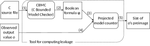
Figure 3: Reduction of computing dynamic leakage to model counting

Pluggability There are several parts in the framework above that can be flexibly changed to utilize the strength of different tools and/or approaches. Firstly, the projected model counter at (5) could be either a projected $\sharp$SAT solver (e.g., SharpCDCL) or a $\sharp$SMT solver (e.g., aZ3). Consequently, a formula at (3) could be either a SAT constraints (e.g., a Boolean formula in DIMACS format) or a SMT constraints (e.g., a formula in SMTLIB format) generated by CBMC. Moreover, this framework can be extended to different programming languages other than C, such as Java, having JPF [26] and KEY [12] as two well-known counterparts of CBMC. In the next section, we are showing experimental results in which we tried several set-ups of tools in this framework to observe the differences.

5 Experiments

We conducted some experiments to investigate the flexibility of the framework to reduce computing dynamic leakage to model counting introduced in the previous section, as well as the scalability of this method. For the simplicity to achieve this purpose, we restricted to calculate dynamic leakage for deterministic programs with uniformly distributed input. Toward the analysis in more general cases and possibilities on performance improvement, we give some discussion and leave it as one of future work.

5.1 Overview

All experiments were done in a same PC with the following specification: core i7-6500U, CPU@2.5GHz x 4, 8GB RAM, Ubuntu 18.04 64 bits. We set one hour as time-out and interrupted execution whenever the running time exceeds this duration. The model counters we used are described below.

• aZ3: a $\sharp$SMT solver developed by Phan et al. [22], which is built on top of the state-of-the-art SMT solver Z3. We used an improved version of aZ3 which is developed by Nakashima et al. [21]. It allows specifying variables of interest, which is equivalent to projection in SAT-based model counter.

• SharpCDCL: a $\sharp$SAT solver with capability of projected counting based on Conflict-Driven Clause Learning (CDCL) [33]. The tool finds a new projected model and then adds a clause blocking to find the same model again. It enumerates all projected models by repeating that.

• DSharp-p: another $\sharp$SAT solver based on d-DNNF format [20]. The tool first translates a given formula into d-DNNF format. It is known that, once given a d-DNNF format of constraints, it takes only linear time to the size of the formula to count models of those constraints. We used an extended version with the capability of projected counting which is added by Klebanov et al. [15, 30].

• GPMC: a projected model counter built on top of the SAT solver glucose [31], in which component analysis and caching used in the model counter SharpSAT are implemented [32].

The benchmarks are taken from previous researches about QIF analysis with most of them are taken from benchmarks of aZ3 [22], except bin_search32.c which is taken from [18]. The difference between the ordinary QIF analysis and dynamic leakage quantification is that the former is not interested in an observed output value, but the latter is. Therefore, for the purpose of these experiments, we augmented the original benchmarks with additional information about concrete values of public output (public input also if there is some). Because we assume deterministic programs with uniformly distributed input, $\mbox{QIF1}(o)=\mbox{QIF2}(o)=\log\frac{|{\cal S}|}{|\mbox{pre}_{P}(o)|}$ by Theorem 2.1. Hence, without loss of precision in comparison, we consider counting $\mbox{pre}_{P}(o)$ as the final goal of these experiments.

5.2 Results

Table 2 shows execution time of model counting based on the four different model counters, in which t/o indicates that the experiment was interrupted because of time-out and - means the counter gave a wrong answer (i.e., only DSharp-p miscounted for UNSAT cases, probably because the tool does assume input formula to be satisfiable). By eliminating parsing time from the comparison, we measured only time needed to count models.

According to the experimental results, aZ3-based model counting did not win the fastest for any benchmark, and moreover its execution time is always at least ten times slower than the best. On the other hand, DSharp-p seems to take much time to translate formulas into d-DNNF format for dining6/50.c and grade.c, and gave wrong answers for mix_duplicate.c and sanity_check.c, the number of models of which are 0, i.e., unsatisfiable. By and large, aZ3 and DSharp-p can hardly take advantage to the other tools, SharpCDCL and GPMC, in dynamic leakage quantification. Though SharpCDCL won 8 out of 14 benchmarks, the difference between the tools in those cases are not significant, yet the execution times are too short that it can be fluctuated by insignificant parameters. Therefore, it is better to look at long run benchmarks, grade.c and masked_copy.c. In both cases, GPMC won by 9.7 times and 287.9 times respectively. The execution times as well as the difference in those two cases are significant. We also noticed that, those two cases have 65,536 and 65 models, which are the two biggest counts among the benchmarks. The more the number of the models is, the bigger is the difference between execution times of GPMC and SharpCDCL. Hence, we can empirically conclude that GPMC-based works much better than SharpCDCL-based in cases the number of models is large, while not so worse in other cases.

By implementing the prototype, we reaffirmed the possibility of automatically computing QIF1 and QIF2. Speaking of scalability, despite of small LOC (Lines of Code), there is still the case of grade.c (48 lines) for which all settings take longer than one minute, a very long time from the viewpoint of runtime analysis, to count models. There are several directions to improve the current performance which we leave as one of future work. First, because dynamic leakage should be calculated repeatedly for different observed outputs but a same program, we can leverage such an advantage of d-DNNF that while transforming to a d-DNNF format takes time, the model counting can be done in linear time once a d-DNNF format is obtained. That is, we generate merely once in advance a d-DNNF format of the constraints representing the program under analysis, then each time an observed output value is given, we make only small modification and count models in linear time to the size of the constraints. The difficulty of this direction lies in how to augment the information of observed output to the generated d-DNNF without breaking its d-DNNF structure. Another direction is to loose the required precision to accept approximate count. This could be done by counting on existing approximate model counters.

Table 2: Counting result and execution time (ms) of different settings

Benchmark	Count	aZ3	SharpCDCL	DSharp-p	GPMC
bin_search32	1	781	37	52	9
crc8	32	303	11	31	36
crc32	8	294	8	32	32
dining6	6	1,305	44	t/o	49
dining50	50	t/o	199	t/o	193
electronic_purse	5	525	137	9,909	223
grade	65	2,705,934	910,655	t/o	93,445
implicit_flow	1	253	15	31	33
masked_copy	65,536	t/o	9,214	30	32
mix_duplicate	0	241	12	-	4
population_count	32	477	19	37	34
sanity_check	0	247	13	-	8
sum_query	3	310	20	31	35
ten_random_outputs	1	249	18	32	34

5.3 Toward general cases

In order to calculate QIF1 and QIF2 for a probabilistic program with a non-uniform input distribution, we must identify projected models of the Boolean formula, rather than the number of the models, to obtain the probabilities determined by them in general. GPMC, specialized for model counting, does not compute the whole part of each model explicitly. Hence, GPMC is not appropriate for a calculation of the probability depending on the concrete models. On the other hand, sharpCDCL basically enumerates all projected models, and thus we think we can extend it as follows to compute QIF1 and QIF2 in general cases.

To calculate QIF1 for a probabilistic program with a non-uniform input distribution, we can replace each probabilistic choice in a give program with a non-deterministic choice as stated in Section 4, and then enumerate projected models with respect to the input variables, summing up the probabilities of the corresponding input values.

As for QIF2, we have to calculate not only the probabilities of possible input values but also those of possible execution paths reachable to the observed output. To achieve this, in addition to the replacement of probabilistic choices with non-deterministic choices, we may insert variables to remember which branch is chosen at each of the non-deterministic choices. Then, given a projected model of the Boolean formula generated from the modified source code with respect to the input variables and the additional choice variables, we can get to know a possible input value and an execution path from the projected model. For a possible input value $s$, $p(o|s)$ is the sum of the probabilities of all possible execution paths from $s$ to the observed $o$.

6 Conclusion

In this paper, we summarize three requirements as criteria for reasonable dynamic leakage definitions to follow. Also we defined two novel ones both of which satisfy all the criteria and have understandable explanations of the background perspectives. Besides giving proof of some of their characteristics, we gave results on the hardness of computing dynamic leakage under those definitions for three classes of Boolean programs, including loop-free, while and recursive. Despite of the hardness, we introduced a framework to reduce the problems to model counting, which gets much attention from researchers from various fields of interest. Based on that framework, we implemented a prototype and conducted some experiments to verify flexibility and scalability of the framework. Lastly, we gave some discussion on how to improve the performance and the whole picture of computing dynamic leakage in general cases.
Beyond this paper, we leave the following as future work: (1) utilizing the strength of d-DNNF format to improve calculation performance, (2) approaching those problems in terms of approximated calculation and (3) tackling the problems under more general assumptions.

References

- [1] R. Alur, K. Etessami, M. Yannakakis, Analysis of recursive state machines, 13th Intenational Conference on Computer-Aided Verification (CAV), 2001, 304–313.
- [2] M. S. Alvim, K. Chatzikokolakis, A. McIver, Axioms for information leakage, 29th Computer Security Foundations Symposium (CSF), 2016, 77–92.
- [3] R. A. Aziz, G. Chu, C. Muise, P. Stuckey, #SAT: projection model counting, 18th International Conference on Theory and Applications of Satisfiability Testing (SAT), 2015, 121–137.
- [4] F. Besson, N. Bielova, T. Jensen, Hybrid Monitoring of Attacker Knowledge, 29th Computer Security Foundations Symposium (CSF), 2016, 225–238.
- [5] N. Bielova, Dynamic leakage - a need for a new quantitative information flow measure, ACM Workshop on Programming Languages and Analysis for Security (PLAS), 2016, 83–88.
- [6] F. Biondi, M. A. Enescu, A. Heuser, A. Legay, K. S. Meel, J. Quilbeuf, Scalable approximation of quantitative information flow in programs, Verification, Model Checking, and Abstract Interpretation (VMCAI), 2018, 71–93.
- [7] F. Biondi, Y. Kawamoto, A. Legay, L. M. Traonouez, HyLeak: hybrid analysis tool for information leakage, Automated Technology for Verification and Analysis (ATVA), 2017, 156–163.
- [8] A. Bouajjani, J. Esparza, O. Maler, Reachability analysis of pushdown automata: application to model-checking, 8th International Conference on Concurrency Theory (CONCUR), 1997, 135–150.
- [9] R. Chadha and M. Ummels, The complexity of quantitative information flow in recursive programs, Research Report LSV-2012-15, Laboratoire Spécification & Vérification, École Normale Supérieure de Cachan, 2012.
- [10] T. Chothia, Y. Kawamoto, C. Novakovic, LeakWatch: estimating information leakage from Java programs, 19th European Symposium on Research in Computer Security (ESORICS), 2014, 219–236.
- [11] M. R. Clarkson, A. C. Myers and F. B. Schneider, Quantifying information flow with beliefs, 18th Computer Security Foundations Symposium (CSF), 2009, 655–701.
- [12] A. Darvas, R. Hähnle, D. Sands, A theorem proving approach to analysis of secure information flow, Security in Pervasive Computing (SPC), 2005, 193–209.
- [13] K. Etessami, M. Yannakakis, Recursive Markov chains, stochastic grammars, and monotone systems of nonlinear equations, Journal of ACM (JACM), Vol. 56, Issue 1, Jan 2009.
- [14] J. A. Goguen, J. Meseguer, Security policies and security models, IEEE Symposium on Security and Privacy (SP), 1982, 11–20.
- [15] V. Klebanov, N. Manthey, C. Muise, SAT-based analysis and quantification of information flow in programs, Quantitative Evaluation of Systems (QEST), 2013, 177-192.
- [16] B. Köpf, A. Rybalchenko, Approximation and randomization for quantitative information flow analysis, 23rd Computer Security Foundations Symposium (CSF), 2010, 3–14.
- [17] S. McCamant, M. D. Ernst, Quantitative information flow as network flow capacity, ACM SIGPLAN Conference on Programming Language Design and Implementation (PLDI), 2008, 193–205.
- [18] Z. Meng, G. Smith, Calculating bounds on information leakage using two-bit patterns, 6th Workshop on Programming Languages and Analysis for Security (PLAS), 2011, 1–12.
- [19] M. Mitzenmacher, E. Upfal, Probability and computing: randomized algorithms and probabilistic analysis, Cambridge, 2005, 167–173.
- [20] C. Muise, S. A. McIlraith, J. C. Beck, E. Hsu, DSHARP: fast d-DNNF compilation with sharpSAT, Advances in Artificial Intelligence (AI), 2012, 356–361.
- [21] S. Nakashima, B. T. Chu, K. Hashimoto, M. Sakai, H. Seki, Efficiency improvement in SMT-based quantitative information flow analysis, IEICE Technical Report, SS2016-26, Vol. 116, No. 277, 2016, 49–54.
- [22] Q. S. Phan, P. Malacaria, All-solution satisfiability modulo theories: applications, algorithms and benchmarks, 10th International Conference on Availability, Reliability and Security (ARES), 2015, 100–109.
- [23] G. Smith, On the foundations of quantitative information flow, 12th International Conference on Foundations of Software Science and Computational Structures (FOSSACS), 2009, 288–302.
- [24] R. Suzuki, K. Hashimoto, M. Sakai, Improvement of projected model-counting solver with component decomposition using SAT solving in components, JSAI Technical Report, SIG-FPAI-506-07, 2017, 31–36 (in Japanese).
- [25] C. G. Val, M. A. Enescu, S. Bayless, W. Aiello, A. J. Hu, Precisely measuring quantitative information flow: 10k lines of code and beyond, IEEE European Symposium on Security and Privacy (EuroSP), 2016, 31–46.
- [26] W. Visser, K. Havelund, G. Brat, S. J. Park, F. Lerda, Model checking programs, Automated Software Engineering (ASE), Vol. 10, Issue 2, 2003, 203–232.
- [27] H. Yasuoka, T. Terauchi, Quantitative information flow - verification hardness and possibilities, 23rd Computer Security Foundations Symposium (CSF), 2010, 15–27.
- [28] H. Yasuoka, T. Terauchi, On bounding problems of quantitative information flow, Journal of Computer Security (JCS), Vol. 19, 2011 November, 1029–1082.
- [29] C Bounded Model Checker, https://www.cprover.org/cbmc.
- [30] DSharp-p, https://formal.iti.kit.edu/~klebanov/software/
- [31] Glucose SAT Solver, https://www.labri.fr/perso/lsimon/glucose.
- [32] GPMC, https://www.trs.css.i.nagoya-u.ac.jp/~k-hasimt/tools/gpmc.html.
- [33] SharpCDCL, http://tools.computational-logic.org/content/sharpCDCL.php.