Exponential Integrators for Stochastic Maxwell’s Equations Driven by Itô Noise

Abstract

This article presents explicit exponential integrators for stochastic Maxwell’s equations driven by both multiplicative and additive noises. By utilizing the regularity estimate of the mild solution, we first prove that the strong order of the numerical approximation is $\frac{1}{2}$ for general multiplicative noise. Combing a proper decomposition with the stochastic Fubini’s theorem, the strong order of the proposed scheme is shown to be $1$ for additive noise. Moreover, for linear stochastic Maxwell’s equation with additive noise, the proposed time integrator is shown to preserve exactly the symplectic structure, the evolution of the energy as well as the evolution of the divergence in the sense of expectation. Several numerical experiments are presented in order to verify our theoretical findings.

60H35, 60H15, 35Q61.

1 Introduction

In the context of electromagnetism, a common way to model precise microscopic origins of randomness (such as thermal motion of electrically charged micro-particles) is by means of stochastic Maxwell’s equations [35]. Further applications of stochastic Maxwell’s equations are: In [32], a stochastic model of Maxwell’s field equations in $1+1$ dimension is shown to be a simple modification of a random walk model due to Kac, which provides a basis for the telegraph equations. The work [27] studies the propagation of ultra-short solitons in a cubic nonlinear medium modeled by nonlinear Maxwell’s equations with stochastic variations of media. To simulate a coplanar waveguide with uncertain material parameters, time-harmonic Maxwell’s equations are considered in [4]. For linear stochastic Maxwell’s equations driven by additive noise, the work [21] proves that the problem is a stochastic Hamiltonian partial differential equation whose phase flow preserves the multi-symplectic geometric structure. In addition, the averaged energy along the flow increases linearly with respect to time and the flow preserves the divergence in the sense of expectation, see [10]. Let us finally mention that linear stochastic Maxwell’s equations are relevant in various physical applications, see e.g. [35, Chapter 3].

We now review the literature on the numerical discretisation of stochastic Maxwell’s equations. The work [41] performs a numerical analysis of the finite element method and discontinuous Galerkin method for stochastic Maxwell’s equations driven by colored noise. A stochastic multi-symplectic method for $3$ dimensional problems with additive noise, based on stochastic variational principle, is studied in [21]. In particular, it is shown that the implicit numerical scheme preserves a discrete stochastic multi-symplectic conservation law. The work [10] inspects geometric properties of the stochastic Maxwell’s equation with additive noise, namely the behavior of averaged energy and divergence, see below for further details. Especially, the authors of [10] investigate three novel stochastic multi-symplectic (implicit in time) methods preserving discrete versions of the averaged divergence. None of the proposed numerical schemes exactly preserve the behavior of the averaged energy. The work [22] proposes a stochastic multi-symplectic wavelet collocation method for the approximation of stochastic Maxwell’s equations with multiplicative noise (in the Stratonovich sense). For the same stochastic Maxwell’s equation as the one considered in this paper (see below for a precise definition), the recent reference [8] shows that the backward Euler–Maruyama method converges with mean-square convergence rate $\frac{1}{2}$. Finally, the preprint [9] studies implicit Runge–Kutta schemes for stochastic Maxwell’s equation with additive noise. In particular, a mean-square convergence of order $1$ is obtained.

In the present paper, we construct and analyse an exponential integrator for stochastic Maxwell’s equations which is explicit (thus computationally more efficient than the above mentioned time integrators) and which enjoys excellent long-time behavior. Observe that exponential integrators are widely used for efficient time integrations of deterministic differential equations, see for instance [18, 7, 19, 12] and more specially [37, 31, 24, 39, 33] and references therein for Maxwell-type equations. In recent years, exponential integrators have been analysed in the context of stochastic (partial) differential equations (S(P)DEs). Without being too exhaustive, we mention analysis and applications of such numerical schemes for the following problems: stochastic differential equations [36, 25, 26]; stochastic parabolic equations [23, 29, 5, 15, 3]; stochastic Schrödinger equations [1, 11, 16]; stochastic wave equations [13, 40, 14, 2, 34] and references therein.

The main contributions of the present paper are:

• a strong convergence analysis of an explicit exponential integrator for stochastic Maxwell’s equations in $\mathbb{R}^{3}$. By making use of regularity estimates of the exact and numerical solutions, the strong convergence order is shown to be $\frac{1}{2}$ for general multiplicative noise. Furthermore, by using a proper decomposition and stochastic Fubini’s theorem, we prove that the strong convergence order of the proposed scheme can achieve $1$.

• an analysis of long-time conservation properties of an explicit exponential integrator for linear stochastic Maxwell’s equations driven by additive noise. Especially, we show that the proposed explicit time integrator is symplectic and satisfies a trace formula for the energy for all times, i. e. the linear drift of the averaged energy is preserved for all times. In addition, the numerical solution preserves the averaged divergence. This shows that the exponential integrator inherits the geometric structure and the dynamical behavior of the flow of the linear stochastic Maxwell’s equations. This is not the case for classical time integrators such as Euler–Maruyama type schemes.

• an efficient numerical implementation of two-dimensional models of stochastic Maxwell’s equations by explicit time integrators.

We would like to remark that the proofs of strong convergence for the exponential integrator use similar ideas present in various proofs of strong convergence from the literature. But, to the best of our knowledge, the present paper offers the first explicit time integrator for linear stochastic Maxwell’s equations that is of strong order $1$, symplectic, exactly preserves the linear drift of the averaged energy, and preserves the averaged divergence for all times. A weak convergence analysis of the proposed scheme for stochastic Maxwell’s equations driven by multiplicative noise will be reported elsewhere.

An outline of the paper is as follows. Section 2 sets notations and introduces the stochastic Maxwell’s equation. This section also presents assumptions to guarantee existence and uniqueness of the exact solution to the problem and shows its Hölder continuity. The exponential integrator for stochastic Maxwell’s equation is introduced in Section 3, where we also prove its strong order of convergence for additive and multiplicative noise. In Section 4, we show that the proposed scheme has several interesting geometric properties: it preserves the evolution laws of the averaged energy, the evolution laws of the divergence, and the symplectic structure of the original linear stochastic Maxwell’s equations with additive noise. We conclude the paper by presenting numerical experiments supporting our theoretical results in Section 5.

2 Well-posedness of stochastic Maxwell’s equations

We consider the stochastic Maxwell’s equation driven by multiplicative Itô noise

(1) $$\begin{split}\text{d}\mathbb{U}&=A\mathbb{U}\,\text{d}t+\mathbb{F}(\mathbb{U})\,\text{d}t+\mathbb{G}(\mathbb{U})\,\text{d}W,\quad{t}\;{\in}\;(0,+\infty),\\ \mathbb{U}(0)&=(\mathbf{E}_{0}^{\top},\mathbf{H}_{0}^{\top})^{\top}\end{split}$$

supplemented with the boundary condition of a perfect conductor $\mathbf{n}\times\mathbf{E}=0$ as in [21]. Here, $\mathbb{U}=(\mathbf{E}^{\top},\mathbf{H}^{\top})^{\top}$, is $\mathbb{R}^{6}$-valued function whose domain $\mathcal{O}$ is a bounded and simply connected domain in $\mathbb{R}^{3}$ with smooth boundary $\partial\mathcal{O}$. The unit outward normal vector to $\partial\mathcal{O}$ is denoted by $\mathbf{n}$. Moreover, $\text{d}W$ stands for the formal time derivative of a $Q$-Wiener process $W$ on a stochastic basis $(\Omega,\mathscr{F},\{\mathscr{F}_{t}\}_{t\geq 0},\mathbb{P})$. The $Q$-Wiener process can be written as $W({\bf x},t)=\sum\limits_{k\in\mathbb{N}_{+}}Q^{\frac{1}{2}}e_{k}({\bf x})\beta_{k}(t)$, where $\{\beta_{k}\}_{k\in\mathbb{N}_{+}}$ is a sequence of mutually independent and identically distributed $\mathbb{R}$-valued standard Brownian motions; $\{e_{k}\}_{k\in\mathbb{N}_{+}}$ is an orthonormal basis of $U:=\mathcal{L}^{2}(\mathcal{O};\mathbb{R})$ consisting of eigenfunctions of a symmetric, nonnegative and of finite trace linear operator $Q$, i. e., $Qe_{k}=\eta_{k}e_{k}$, with $\eta_{k}\geq 0$ for $k\in\mathbb{N}_{+}$. Assumptions on $\mathbb{F}$ and $\mathbb{G}$ are provided below.

The Maxwell’s operator $A$ is defined by

(2) $$A\begin{pmatrix}\mathbf{E}\\ \mathbf{H}\end{pmatrix}:=\begin{pmatrix}0&\epsilon^{-1}\nabla\times\\ -\mu^{-1}\nabla\times&0\end{pmatrix}\begin{pmatrix}\mathbf{E}\\ \mathbf{H}\end{pmatrix}=\begin{pmatrix}\epsilon^{-1}\nabla\times\mathbf{H}\\ -\mu^{-1}\nabla\times\mathbf{E}\end{pmatrix}.$$

It has the domain $D(A):=H_{0}(\mathrm{curl},\mathscr{O})\times H(\mathrm{curl},\mathscr{O})$, where

$$H(\mathrm{curl},\mathscr{O}):=\{\mathbf{U}\in(\mathcal{L}^{2}(\mathscr{O}))^{3}:\nabla\times\mathbf{U}\in(\mathcal{L}^{2}(\mathscr{O}))^{3}\},$$

is termed by the ${\mathrm{curl}}$-space and

$$H_{0}(\mathrm{curl},\mathscr{O}):=\{\mathbf{U}\in H(\mathrm{curl},\mathscr{O}):\mathbf{n}\times\mathbf{U}|_{\partial\mathscr{O}}=\mathbf{0}\}$$

is the subspace of $H(\mathrm{curl},\mathscr{O})$ with zero tangential trace. In addition, $\epsilon$ and $\mu$ are bounded and uniformly positive definite functions:

$$\epsilon,\mu\in\mathcal{L}^{\infty}(\mathscr{O}),\quad\epsilon,\mu\geq\kappa>0$$

with $\kappa$ being a positive constant. These conditions on $\epsilon,\mu$ ensure that the Hilbert space $V:=(\mathcal{L}^{2}(\mathscr{O}))^{3}\times(\mathcal{L}^{2}(\mathscr{O}))^{3}$ is equipped with the weighted scalar product

$$\left\langle\begin{pmatrix}\mathbf{E}_{1}\\ \mathbf{H}_{1}\end{pmatrix},\begin{pmatrix}\mathbf{E}_{2}\\ \mathbf{H}_{2}\end{pmatrix}\right\rangle_{V}=\int_{\mathscr{O}}\left(\mu\langle\mathbf{H}_{1},\mathbf{H}_{2}\rangle+\epsilon\langle\mathbf{E}_{1},\mathbf{E}_{2}\rangle\right)\,\text{d}{\bf x},$$

where $\langle\cdot,\cdot\rangle$ stands for the standard Euclidean inner product. This weighted scalar product is equivalent to the standard inner product on $(\mathcal{L}^{2}(\mathcal{O}))^{6}$. Moreover, the corresponding norm, which stands for the electromagnetic energy of the physical system, induced by this inner product reads

$$\left\|\begin{pmatrix}\mathbf{E}\\ \mathbf{H}\end{pmatrix}\right\|_{V}^{2}=\int_{\mathscr{O}}\left(\mu\|\mathbf{H}\|^{2}+\epsilon\|\mathbf{E}\|^{2}\right)\,\text{d}{\bf x}$$

with $\|\cdot\|$ being the Euclidean norm. Based on the norm $\|\cdot\|_{V}$, the associated graph norm of $A$ is defined by

$$\|\mathbb{V}\|_{D(A)}^{2}:=\|\mathbb{V}\|_{V}^{2}+\|A\mathbb{V}\|_{V}^{2}.$$

It is well known that Maxwell’s operator $A$ is closed and that $D(A)$ equipped with the graph norm is a Banach space, see e.g. [30]. Moreover, $A$ is skew-adjoint, in particular, for all $\mathbb{V}_{1},\mathbb{V}_{2}\in D(A)$,

$$\langle A\mathbb{V}_{1},\mathbb{V}_{2}\rangle_{V}=-\langle\mathbb{V}_{1},A\mathbb{V}_{2}\rangle_{V}.$$

In addition, the operator $A$ generates a unitary $C_{0}$-group $\mathbf{S}(t):=\exp(tA)$ via Stone’s theorem, see for example [17]. According to the definition of unitary groups, one has

(3) $$\|\mathbf{S}(t)\mathbb{V}\|_{V}=\|\mathbb{V}\|_{V}\quad\text{for all}\quad\mathbb{V}\in V,$$

which means that the electromagnetic energy is preserved, for Maxwell’s operator, see [20]. Besides, the unitary group $\mathbf{S}(t)$ satisfies the following properties which will be made use of in the next section.

Lemma 2.1 (Theorem 3 with $\mathbf{q=0}$ in [6]).

For the semigroup $\{\mathbf{S}(t);t\geq 0\}$ on $V$, it holds that

(4) $$\|\mathbf{S}(t)-Id\|_{L\left(D(A);V\right)}\leq Ct,$$

where the constant $C$ does not depend on $t$. Here, $L(D(A);V)$ denotes the space of bounded linear operators from $D(A)$ to $V$.

Observe that, throughout the paper, $C$ stands for a constant that may vary from line to line.

For two real-valued separable Hilbert spaces $(H_{1},\langle\cdot,\cdot\rangle_{H_{1}},\|\cdot\|_{H_{1}})$ and $(H_{2},\langle\cdot,\cdot\rangle_{H_{2}},\|\cdot\|_{H_{2}})$, we denote the set of Hilbert–Schmidt operators from $H_{1}$ to $H_{2}$ by $\mathcal{L}_{2}(H_{1},H_{2})$. It will be equipped with the norm

$$\|\Gamma\|^{2}_{\mathcal{L}_{2}(H_{1},H_{2})}:=\sum\limits_{i=1}^{\infty}\|\Gamma\phi_{i}\|_{H_{2}}^{2},$$

where $\{\phi_{i}\}_{i\in\mathbb{N}_{+}}$ is any orthonormal basis of $H_{1}$. Furthermore, let $Q^{\frac{1}{2}}$ be the unique positive square root of the linear operator $Q$ (defining the noise $W$). We also introduce the separable Hilbert space $U_{0}:=Q^{\frac{1}{2}}U$ endowed with the inner product $\langle u_{1},u_{2}\rangle_{U_{0}}:=\langle Q^{-\frac{1}{2}}u_{1},Q^{-\frac{1}{2}}u_{2}\rangle_{U}$ for $u_{1},u_{2}\in U_{0}$, where we recall that $U=\mathcal{L}^{2}(\mathcal{O};\mathbb{R})$.

Lemma 2.2.

As a consequence of Lemma 2.1, for any $\Phi\in\mathcal{L}_{2}\left(U_{0},D(A)\right)$ and any $t\geq 0,$ we have

(5) $$\|\left(\mathbf{S}(t)-Id\right)\Phi\|_{\mathcal{L}_{2}(U_{0},V)}\leq Ct\|\Phi\|_{\mathcal{L}_{2}(U_{0},D(A))}.$$

Proof Thanks to Lemma 2.1 and the definition of the Hilbert–Schmidt norm, we know that, for $\{e_{k}\}_{k\in\mathbb{N}_{+}}$ an orthonormal basis of $U$,

$$\|\left(\mathbf{S}(t)-Id\right)\Phi\|_{\mathcal{L}_{2}(U_{0},V)}^{2} =\sum\limits_{k\in\mathbb{N}_{+}}\|\left(\mathbf{S}(t)-Id\right)\Phi Q^{\frac{1}{2}}e_{k}\|^{2}_{V}$$

$$\leq Ct^{2}\sum\limits_{k\in\mathbb{N}_{+}}\|\Phi Q^{\frac{1}{2}}e_{k}\|^{2}_{D(A)}\leq Ct^{2}\|\Phi\|_{\mathcal{L}_{2}(U_{0},D(A))}^{2},$$

which proves the claim. $\square$

To guarantee existence and uniqueness of strong solutions to (1), we make the following assumptions:

Assumption 2.1 (Coefficients).

Assume that the coefficients of Maxwell’s operator (2) satisfy

$$\epsilon,\mu\in\mathcal{L}^{\infty}(\mathscr{O}),\quad\epsilon,\mu\geq\kappa>0$$

with some positive constant $\kappa$.

Assumption 2.2 (Initial value).

The initial value $\mathbb{U}(0)$ of the stochastic Maxwell’s equation (1) is a $D(A)$-valued stochastic process with $\mathbb{E}\left[\|\mathbb{U}(0)\|^{p}_{D(A)}\right]<\infty$ for any $p\geq 1$.

Assumption 2.3 (Nonlinearity).

We assume that the operator $\mathbb{F}\colon V\to V$ is continuous and that there exists constants $C_{\mathbb{F}},C_{\mathbb{F}}^{1}>0$ such that

$$\|\mathbb{F}(\mathbb{V}_{1})-\mathbb{F}(\mathbb{V}_{2})\|_{V}\leq C_{\mathbb{F}}\|\mathbb{V}_{1}-\mathbb{V}_{2}\|_{V},\quad\mathbb{V}_{1},\mathbb{V}_{2}\in V,$$

$$\|\mathbb{F}(\mathbb{V}_{1})-\mathbb{F}(\mathbb{V}_{2})\|_{D(A)}\leq C_{\mathbb{F}}^{1}\|\mathbb{V}_{1}-\mathbb{V}_{2}\|_{D(A)},\quad\mathbb{V}_{1},\mathbb{V}_{2}\in D(A),$$

$$\|\mathbb{F}(\mathbb{V})\|_{V}\leq C_{\mathbb{F}}(1+\|\mathbb{V}\|_{V}),\quad\mathbb{V}\in V,$$

$$\|\mathbb{F}(\mathbb{V})\|_{D(A)}\leq C_{\mathbb{F}}^{1}\left(1+\|\mathbb{V}\|_{D(A)}\right),\quad\mathbb{V}\in D(A).$$

Assumption 2.4 (Noise).

We assume that the operator $\mathbb{G}\colon V\to\mathcal{L}_{2}(U_{0},V)$ satisfies

(6) $$\begin{split}&\|\mathbb{G}(\mathbb{V}_{1})-\mathbb{G}(\mathbb{V}_{2})\|_{\mathcal{L}_{2}(U_{0},V)}\leq C_{\mathbb{G}}\|\mathbb{V}_{1}-\mathbb{V}_{2}\|_{V},\;\mathbb{V}_{1},\mathbb{V}_{2}\in V,\\ &\|\mathbb{G}(\mathbb{V}_{1})-\mathbb{G}(\mathbb{V}_{2})\|_{\mathcal{L}_{2}(U_{0},{D(A)})}\leq C_{\mathbb{G}}^{1}\|\mathbb{V}_{1}-\mathbb{V}_{2}\|_{D(A)},\;\mathbb{V}_{1},\mathbb{V}_{2}\in D(A),\\ &\|\mathbb{G}(\mathbb{V})\|_{\mathcal{L}_{2}(U_{0},V)}\leq C_{\mathbb{G}}(1+\|\mathbb{V}\|_{V}),\quad\mathbb{V}\in V,\\ &\|\mathbb{G}(\mathbb{V})\|_{\mathcal{L}_{2}(U_{0},D(A))}\leq C_{\mathbb{G}}^{1}(1+\|\mathbb{V}\|_{D(A)}),\quad\mathbb{V}\in D(A),\end{split}$$

where $C_{\mathbb{G}},C_{\mathbb{G}}^{1}>0$ may depend on the operator $Q$. We recall that $\mathcal{L}_{2}(U_{0},V)$ and $\mathcal{L}_{2}(U_{0},D(A))$ denote the spaces of Hilbert–Schmidt operators from $U_{0}$ to $V$, resp. to $D(A)$.

We now present two examples of an operator $\mathbb{G}$ verifying Assumption 2.4 (we only prove one of the inequality in (LABEL:con;G), the others follow in a similar way).

For the first example (inspired by [21]), let $\mathcal{O}=[0,1]^{3}$, $\epsilon=\mu=1$ and consider $\mathbb{G}\equiv(\lambda_{1},\lambda_{1},\lambda_{1},\lambda_{2},\lambda_{2},\lambda_{2})^{T}$ for two real numbers $\lambda_{1}$ and $\lambda_{2}$. The stochastic Maxwell’s equation (1) then becomes an SPDE driven by additive noise. In this case, one chooses the orthonormal basis of $U$ to be $\sin(i\pi x_{1})\sin(j\pi x_{2})\sin(k\pi x_{3})$, for $i,j,k\in\mathbb{N}_{+}$, and $x_{1},x_{2},x_{3}\in[0,1]$. Assuming for example that $\|Q^{\frac{1}{2}}\|_{\mathcal{L}_{2}(U,\mathcal{H}^{1}_{0})}<\infty$, where $\mathcal{H}^{1}_{0}:=\mathcal{H}^{1}_{0}(\mathcal{O})=\{u\in\mathcal{H}^{1}(\mathcal{O})\colon u=0\>\>\text{on}\>\>\partial\mathcal{O}\}$, one can get that $\mathbb{G}Q^{\frac{1}{2}}\mathbb{V}\in D(A)$ for all $\mathbb{V}\in D(A)$ and thus the last inequality in (LABEL:con;G) holds.

For the second example (inspired by [8]), consider $\mathbb{G}(\mathbb{V})=\mathbb{V}$ for $\mathbb{V}\in V$, the domain $\mathcal{O}=[0,1]^{3}$ and $\epsilon=\mu=1$. Taking the same orthonormal basis as above, and assuming in addition that $Q^{\frac{1}{2}}\in\mathcal{L}_{2}(U,\mathcal{H}^{1+\gamma}(\mathcal{O}))$ with $\gamma>\frac{3}{2}$, one gets for instance

(7) $$\begin{split}&\|\mathbb{G}(\mathbb{V})\|_{\mathcal{L}_{2}(U_{0},D(A))}\leq C\|Q^{\frac{1}{2}}\|_{\mathcal{L}_{2}(U,\mathcal{H}^{1+\gamma})}(1+\|\mathbb{V}\|_{D(A)}).\end{split}$$

Using the definition of the graph norm one gets

$$\|\mathbb{G}(\mathbb{V})\|_{\mathcal{L}_{2}(U_{0},D(A))}^{2} =\sum\limits_{k\in\mathbb{N}_{+}}\|\mathbb{V}Q^{\frac{1}{2}}e_{k}\|_{V}^{2}+\sum\limits_{k\in\mathbb{N}_{+}}\|A(\mathbb{V}Q^{\frac{1}{2}}e_{k})\|_{V}^{2}.$$

Denoting $\mathbb{V}=({\bf E}_{\mathbb{V}}^{T},{\bf H}_{\mathbb{V}}^{T})^{T}$ and using the definition of the operator $A$, one obtains

$$\|\mathbb{G}(\mathbb{V})\|_{\mathcal{L}_{2}(U_{0},D(A))}^{2}$$

$$=\sum\limits_{k\in\mathbb{N}_{+}}\sum_{i=1,2,3}\|{\bf E}_{\mathbb{V}}^{i}Q^{\frac{1}{2}}e_{k}\|_{U}^{2}+\sum\limits_{k\in\mathbb{N}_{+}}\sum_{i=1,2,3}\|{\bf H}_{\mathbb{V}}^{i}Q^{\frac{1}{2}}e_{k}\|_{U}^{2}$$

$$\quad+\sum\limits_{k\in\mathbb{N}_{+}}\Big{(}\|\nabla\times({\bf E}_{\mathbb{V}}Q^{\frac{1}{2}}e_{k})\|_{U^{3}}^{2}+\|\nabla\times({\bf H}_{\mathbb{V}}Q^{\frac{1}{2}}e_{k})\|_{U^{3}}^{2}\Big{)}$$

$$\leq C\sum\limits_{k\in\mathbb{N}_{+}}\|Q^{\frac{1}{2}}e_{k}\|_{L^{\infty}(\mathcal{O})}^{2}\|\mathbb{V}\|_{V}^{2}+\sum\limits_{k\in\mathbb{N}_{+}}\Big{(}\|\nabla\times({\bf E}_{\mathbb{V}}Q^{\frac{1}{2}}e_{k})\|_{U^{3}}^{2}+\|\nabla\times({\bf H}_{\mathbb{V}}Q^{\frac{1}{2}}e_{k})\|_{U^{3}}^{2}\Big{)}.$$

We now illustrate how to estimate the term $\|\nabla\times({\bf E}_{\mathbb{V}}Q^{\frac{1}{2}}e_{k})\|_{U^{3}}^{2}$ as an example. Using the definition of the curl operator, one gets

$$\|\nabla\times({\bf E}_{\mathbb{V}}Q^{\frac{1}{2}}e_{k})\|_{U^{3}}^{2} =\|\frac{\partial}{\partial x_{2}}({\bf E}_{\mathbb{V}}^{3}Q^{\frac{1}{2}}e_{k})-\frac{\partial}{\partial x_{3}}({\bf E}_{\mathbb{V}}^{2}Q^{\frac{1}{2}}e_{k})\|_{U}^{2}$$

$$\quad+\|\frac{\partial}{\partial x_{1}}({\bf E}_{\mathbb{V}}^{3}Q^{\frac{1}{2}}e_{k})-\frac{\partial}{\partial x_{3}}({\bf E}_{\mathbb{V}}^{1}Q^{\frac{1}{2}}e_{k})\|_{U}^{2}$$

$$\quad+\|\frac{\partial}{\partial x_{1}}({\bf E}_{\mathbb{V}}^{2}Q^{\frac{1}{2}}e_{k})-\frac{\partial}{\partial x_{2}}({\bf E}_{\mathbb{V}}^{1}Q^{\frac{1}{2}}e_{k})\|_{U}^{2}$$

$$\leq C\|Q^{\frac{1}{2}}e_{k}\|^{2}_{L^{\infty}(\mathcal{O})}\Big{(}\|\frac{\partial}{\partial x_{2}}{\bf E}_{\mathbb{V}}^{3}-\frac{\partial}{\partial x_{3}}{\bf E}_{\mathbb{V}}^{2}\|_{U}^{2}+\|\frac{\partial}{\partial x_{1}}{\bf E}_{\mathbb{V}}^{3}-\nabla^{3}{\bf E}_{\mathbb{V}}^{1}\|_{U}^{2}$$

$$\quad+\|\frac{\partial}{\partial x_{1}}{\bf E}_{\mathbb{V}}^{2}-\nabla^{2}{\bf E}_{\mathbb{V}}^{1}\|_{U}^{2}\Big{)}$$

$$\quad+C\Big{(}\|\frac{\partial}{\partial x_{1}}Q^{\frac{1}{2}}e_{k}\|_{L^{\infty}(\mathcal{O})}^{2}+\|\frac{\partial}{\partial x_{2}}Q^{\frac{1}{2}}e_{k}\|_{L^{\infty}(\mathcal{O})}^{2}+\|\frac{\partial}{\partial x_{3}}Q^{\frac{1}{2}}e_{k}\|_{L^{\infty}(\mathcal{O})}^{2}\Big{)}\|{\bf E}_{\mathbb{V}}\|_{U^{3}}^{2}$$

$$\leq C\|Q^{\frac{1}{2}}e_{k}\|^{2}_{L^{\infty}(\mathcal{O})}\|\nabla\times{\bf E}_{\mathbb{V}}\|_{U^{3}}^{2}+C\|\nabla Q^{\frac{1}{2}}e_{k}\|^{2}_{L^{\infty}(\mathcal{O})}\|{\bf E}_{\mathbb{V}}\|_{V}^{2}.$$

Combing the above estimates, we obtain

$$\|\mathbb{G}(\mathbb{V})\|_{\mathcal{L}_{2}(U_{0},D(A))}^{2} \leq C\sum\limits_{k\in\mathbb{N}_{+}}\|Q^{\frac{1}{2}}e_{k}\|_{L^{\infty}(\mathcal{O})}^{2}\bigl{(}\|\mathbb{V}\|_{V}^{2}+\|A\mathbb{V}\|_{V}^{2}\bigr{)}+C\sum\limits_{k\in\mathbb{N}_{+}}\|\nabla Q^{\frac{1}{2}}e_{k}\|_{L^{\infty}(\mathcal{O})}^{2}\|\mathbb{V}\|_{V}^{2}.$$

Using the Sobolev embedding $\mathcal{H}^{\gamma}(\mathcal{O})\hookrightarrow L^{\infty}(\mathcal{O})$ for any $\gamma>\frac{3}{2}$, one finally obtains (LABEL:con1;G) and the linear growth property of $\mathbb{G}$.

The above assumptions suffice to establish well-posedness and regularity results of solutions to (1). This uses similar arguments as, for instance, [28, Theorem 9] (for a more general drift coefficient in (1)) and [8, Corollary 3.1].

Lemma 2.3.

Let $T>0$. Under the Assumptions 2.1-2.4, the stochastic Maxwell’s equation (1) is strongly well posed and its solution $\mathbb{U}$ satisfies

$$\mathbb{E}\left[\sup_{0\leq t\leq T}\|\mathbb{U}(t)\|_{D(A)}^{p}\right]<C\left(1+\mathbb{E}\left[\|\mathbb{U}(0)\|_{D(A)}^{p}\right]\right)$$

for any $p\geq 2$. Here, the constant $C$ depends on $p$, $T$, $Q$, bounds for $\mathbb{F}$ and $\mathbb{G}$, and $\mathbb{U}(0)$.

Subsequently we present a lemma on the Hölder regularity in time of solutions to (1). This result is important in analysing the approximation error of the proposed time integrator in Section 3.

Lemma 2.4.

Let $T>0$. Under the Assumptions 2.1-2.4, the solution $\mathbb{U}$ of the stochastic Maxwell’s equation (1) satisfies

$$\mathbb{E}\left[\|\mathbb{U}(t)-\mathbb{U}(s)\|_{V}^{2p}\right]\leq C|t-s|^{p},$$

for any $0\leq s,t\leq T$, and $p\geq 1$. Here, the constant $C$ depends on $p$, $T$, $Q$, bounds for $\mathbb{F}$ and $\mathbb{G}$, and $\mathbb{U}(0)$.

The proof is very similar to the proof of [8, Proposition 3.2], we omit it for ease of presentation.

Based on the above regularity results for solutions to the stochastic Maxwell’s equation (1), the work [8] shows mean-square convergence order $\frac{1}{2}$ of the backward Euler–Maruyama scheme (in temporal direction). In the next section, we design and analyse an explicit and effective numerical scheme, the exponential integrator, which has the rate of convergence $1$ and preserves many inherent properties of the original problem (in the case of the stochastic Maxwell’s equations with additive noise).

3 Exponential integrators for stochastic Maxwell’s equations and error analysis

This section is concerned with a convergence analysis in strong sense of an exponential integrator for the stochastic Maxwell’s equation (1). We first show an a priori estimate of the numerical solution. Then the strong convergence rate is studied in two cases, first when equation (1) is driven by additive noise and then for multiplicative noise.

Fix a time horizon $T>0$ and an integer $N>0$. Define a stepsize $\Delta t$ such that $T=N\Delta t$. We then construct a uniform partition of the interval $[0,T]$

$$0=t_{0}<t_{1}<\ldots<t_{N-1}<t_{N}=T$$

with $t_{n}=n\Delta t$ for $n=0,\ldots,N$. Next, we consider the mild solution of the stochastic Maxwell’s equation (1) on the small time interval $[t_{k},t_{k+1}]$ (with $\mathbb{U}(t_{k})=\mathbb{U}_{k}$):

$$\mathbb{U}(t_{k+1})=\mathbf{S}(\Delta t)\mathbb{U}_{k}+\int_{t_{k}}^{t_{k+1}}\mathbf{S}(t_{k+1}-s)\mathbb{F}(\mathbb{U}(s))\,\text{d}s+\int_{t_{k}}^{t_{k+1}}\mathbf{S}(t_{k+1}-s)\mathbb{G}(\mathbb{U}(s))\,\text{d}W.$$

By approximating both integrals in the above mild solution at the left end point, one obtains the exponential integrator

(8) $$\mathbb{U}_{k+1}=\mathbf{S}(\Delta t)\mathbb{U}_{k}+\mathbf{S}(\Delta t)\mathbb{F}(\mathbb{U}_{k})\Delta t+\mathbf{S}(\Delta t)\mathbb{G}(\mathbb{U}_{k})\Delta W_{k},$$

where $\Delta W_{k}=\Delta W(t_{k+1})-\Delta W(t_{k})$ stands for Wiener increments. One readily sees that (8) is an explicit numerical approximation of the exact solution $\mathbb{U}(t_{k+1})$ of the stochastic Maxwell’s equation (1).

In order to present a result on the strong error of the exponential integrator (8), we first show an a priori estimate of the numerical solution.

Theorem 3.1.

Under the Assumptions 2.1-2.4, the numerical solution to the stochastic Maxwell’s equation given by the exponential integrator (8) satisfies

$$\mathbb{E}\left[\|\mathbb{U}_{k}\|^{2p}_{D(A)}\right]\leq C(\mathbb{U}_{0},Q,T,p,\mathbb{F},\mathbb{G})$$

for all $p\geq 1$ and $k=0,1,\ldots,N$.

Proof. The numerical approximation given by the exponential integrator can be rewritten as

$$\mathbb{U}_{k} =\mathbf{S}(t_{k})\mathbb{U}(0)+\Delta t\sum\limits_{j=0}^{k-1}\mathbf{S}(t_{k}-t_{j})\mathbb{F}(\mathbb{U}_{j})+\sum\limits_{j=0}^{k-1}\mathbf{S}(t_{k}-t_{j})\mathbb{G}(\mathbb{U}_{j})\Delta W_{j}.$$

Taking norm and expectation leads to, for $p\geq 1$,

$$\mathbb{E}\left[\|\mathbb{U}_{k}\|^{2p}_{D(A)}\right] \leq C\mathbb{E}\left[\|\mathbf{S}(t_{k})\mathbb{U}(0)\|^{2p}_{D(A)}\right]+C\mathbb{E}\left[\left\|\Delta t\sum\limits_{j=0}^{k-1}\mathbf{S}(t_{k}-t_{j})\mathbb{F}(\mathbb{U}_{j})\right\|^{2p}_{D(A)}\right]$$

$$\quad+C\mathbb{E}\left[\left\|\sum\limits_{j=0}^{k-1}\mathbf{S}(t_{k}-t_{j})\mathbb{G}(\mathbb{U}_{j})\Delta W_{j}\right\|^{2p}_{D(A)}\right].$$

For the first term, using the definition of the graph norm and property (3), we obtain

$$\|\mathbf{S}(t_{k})\mathbb{U}(0)\|^{2p}_{D(A)}=\left(\|\mathbf{S}(t_{k})\mathbb{U}(0)\|_{V}+\|\mathbf{S}(t_{k})A\mathbb{U}(0)\|_{V}\right)^{2p}=\|\mathbb{U}(0)\|^{2p}_{D(A)},$$

which leads to $\mathbb{E}\left[\|\mathbf{S}(t_{k})\mathbb{U}(0)\|^{2p}_{D(A)}\right]=\mathbb{E}\left[\|\mathbb{U}(0)\|^{2p}_{D(A)}\right]$. Based on the linear growth property of $\mathbb{F}$ and Hölder’s inequality, the second term is estimated as follows

$$\left\|\Delta t\sum\limits_{j=0}^{k-1}\mathbf{S}(t_{k}-t_{j})\mathbb{F}(\mathbb{U}_{j})\right\|^{2p}_{D(A)}\leq C+C\Delta t^{2p}\left(\sum\limits_{j=0}^{k-1}\|\mathbb{U}_{j}\|_{D(A)}\right)^{2p}$$

$$\leq C+C\Delta t^{2p}k^{2p-1}\sum\limits_{j=0}^{k-1}\|\mathbb{U}_{j}\|_{D(A)}^{2p}.$$

One then obtains

$$\mathbb{E}\left[\left\|\Delta t\sum\limits_{j=0}^{k-1}\mathbf{S}(t_{k}-t_{j})\mathbb{F}(\mathbb{U}_{j})\right\|^{2p}_{D(A)}\right]\leq C+C\Delta t\mathbb{E}\left[\sum\limits_{j=0}^{k-1}\|\mathbb{U}_{j}\|_{D(A)}^{2p}\right].$$

The third term is equivalent to

$$\mathbb{E}\left[\left\|\sum\limits_{j=0}^{k-1}\mathbf{S}(t_{k}-t_{j})\mathbb{G}(\mathbb{U}_{j})\Delta W_{j}\right\|^{2p}_{D(A)}\right] =\mathbb{E}\left[\left\|\int_{0}^{t_{k}}\mathbf{S}\left(t_{k}-[\frac{s}{\Delta t}]\Delta t\right)\mathbb{G}(\mathbb{U}_{[\frac{s}{\Delta t}]\Delta t})\,\text{d}W(s)\right\|^{2p}_{D(A)}\right]$$

with $[\frac{s}{\Delta t}]$ being the integer part of $\frac{s}{\Delta t}$. The Burkholder–Davis–Gundy inequality for stochastic integrals and our assumption on $\mathbb{G}$ give

$$\mathbb{E}\left[\left\|\int_{0}^{t_{k}}\mathbf{S}\left(t_{k}-[\frac{s}{\Delta t}]\Delta t\right)\mathbb{G}(\mathbb{U}_{[\frac{s}{\Delta t}]\Delta t})\,\text{d}W(s)\right\|^{2p}_{D(A)}\right]\leq$$

$$\leq C\mathbb{E}\left[\left(\int_{0}^{t_{k}}\left\|\mathbb{G}(\mathbb{U}_{[\frac{s}{\Delta t}]\Delta t})\right\|_{\mathcal{L}_{2}(U_{0},D(A))}^{2}\,\text{d}s\right)^{p}\right]$$

$$\leq C+C\mathbb{E}\left[\left(\int_{0}^{t_{k}}\left\|\mathbb{U}_{[\frac{s}{\Delta t}]\Delta t}\right\|_{D(A)}^{2}\,\text{d}s\right)^{p}\right]=C+C\mathbb{E}\left[\left(\Delta t\sum\limits_{j=0}^{k-1}\|\mathbb{U}_{j}\|_{D(A)}^{2}\right)^{p}\right].$$

Using Hölder’s inequality, the last term in the above inequality becomes

$$\left(\Delta t\sum\limits_{j=0}^{k-1}\|\mathbb{U}_{j}\|_{D(A)}^{2}\right)^{p}\leq\Delta t^{p}k^{p-1}\sum\limits_{j=0}^{k-1}\|\mathbb{U}_{j}\|_{D(A)}^{2p}.$$

Taking expectation, we then obtain

$$\mathbb{E}\left[\left\|\int_{0}^{t_{k}}\mathbf{S}\left(t_{k}-[\frac{s}{\Delta t}]\Delta t\right)\mathbb{G}(\mathbb{U}(s))\,\text{d}W(s)\right\|^{2p}_{D(A)}\right]\leq C+C\Delta t\sum\limits_{j=0}^{k-1}\mathbb{E}\left[\|\mathbb{U}_{j}\|_{D(A)}^{2p}\right].$$

Altogether, we get that

$$\mathbb{E}\left[\|\mathbb{U}_{k}\|^{2p}_{D(A)}\right]\leq C+C\Delta t\mathbb{E}\left[\sum\limits_{j=0}^{k-1}\|\mathbb{U}_{j}\|_{D(A)}^{2p}\right].$$

A discrete Gronwall inequality concludes the proof. $\square$
Using the above theorem, we arrive at

Corollary 3.1.

Under the same assumptions as in Theorem 3.1, for all $p\geq 1$, there exists a constant $C:=C(\mathbb{U}(0),Q,T,p,\mathbb{F},\mathbb{G})$ such that

(9) $$\mathbb{E}\left[\sup_{0\leq k\leq N}\|\mathbb{U}_{k}\|^{2p}_{D(A)}\right]\leq C.$$

Proof. The main idea to derive the estimate (9) is to properly estimate the stochastic integral

$$\mathbb{E}\left[\sup_{0\leq k\leq N}\left\|\sum\limits_{j=0}^{k-1}\mathbf{S}(t_{k}-t_{j})\mathbb{G}(\mathbb{U}_{j})\Delta W_{j}\right\|^{2p}_{D(A)}\right]=$$

$$=\mathbb{E}\left[\sup_{0\leq k\leq N}\left\|\int_{0}^{t_{k}}\mathbf{S}\left(t_{k}-[\frac{s}{\Delta t}]\Delta t\right)\mathbb{G}(\mathbb{U}_{[\frac{s}{\Delta t}]\Delta t})\,\text{d}W(s)\right\|^{2p}_{D(A)}\right].$$

Based on the unitarity of $S(\cdot)$, Burkholder–Davis–Gundy’s inequality, Hölder’s inequality, and our assumptions on $\mathbb{G}$, the right hand side (RHS) of the above equality becomes

$${\rm RHS} \leq C\mathbb{E}\left[\left(\int_{0}^{T}\left\|\mathbb{G}(\mathbb{U}_{[\frac{s}{\Delta t}]\Delta t})\right\|_{\mathcal{L}_{2}(U_{0},D(A))}^{2}\,\text{d}s\right)^{p}\right]$$

$$\leq C+C\Delta t\sum\limits_{j=0}^{N-1}\mathbb{E}\left[\|\mathbb{U}_{j}\|_{D(A)}^{2p}\right]\leq C,$$

where we use the result of Theorem 3.1 in the last step. The estimations of the other terms in the numerical solution are done in a similar way as in the previous result. $\square$

We are now in position to show the error estimates of the exponential integrator for the stochastic Maxwell’s equation (1) driven by additive noise.

Theorem 3.2.

Let Assumptions 2.1-2.4 hold. Assume in addition that $\mathbb{F}\in C_{b}^{2}(V)$ and $\mathbb{G}$ does not dependent on $\mathbb{U}$. The strong error of the exponential integrator (8) when applied to the stochastic Maxwell’s equation (1) verifies, for all $p\geq 1$,

$$\left(\mathbb{E}\left[\max_{k=0,\ldots,N}\|\mathbb{U}(t_{k})-\mathbb{U}_{k}\|_{V}^{2p}\right]\right)^{\frac{1}{2p}}\leq C\Delta t,$$

where the positive constant $C$ depends on bounds for $\mathbb{F}$ (and its derivatives) and $\mathbb{G}$, as well as on $T$, $p$ and $Q$.

Proof. Let us denote $\epsilon_{k}=\mathbb{U}(t_{k})-\mathbb{U}_{k}$, for $k=0,\ldots,N$. We then have

$$\epsilon_{k+1} =\sum\limits_{j=0}^{k}\int_{t_{j}}^{t_{j+1}}\left(\mathbf{S}(t_{k+1}-s)\mathbb{F}(\mathbb{U}(s))-\mathbf{S}(t_{k+1}-t_{j})\mathbb{F}(\mathbb{U}_{j})\right)\,\text{d}s$$

$$\quad+\sum\limits_{j=0}^{k}\int_{t_{j}}^{t_{j+1}}\left((\mathbf{S}(t_{k+1}-s)-\mathbf{S}(t_{k+1}-t_{j}))\mathbb{G}\right)\,\text{d}W(s)$$

(10) $$=:Err_{1}^{k}+Err_{2}^{k}.$$

We now rewrite the term $Err_{1}^{k}$ as

$$Err_{1}^{k} =\sum\limits_{j=0}^{k}\int_{t_{j}}^{t_{j+1}}\left(\mathbf{S}(t_{k+1}-s)(\mathbb{F}(\mathbb{U}(s))-\mathbb{F}(\mathbb{U}(t_{j})))\right)\,\text{d}s$$

$$\quad+\sum\limits_{j=0}^{k}\int_{t_{j}}^{t_{j+1}}\left(\left(\mathbf{S}(t_{k+1}-s)-\mathbf{S}(t_{k+1}-t_{j})\right)\mathbb{F}(\mathbb{U}(t_{j}))\right)\,\text{d}s$$

$$\quad+\sum\limits_{j=0}^{k}\int_{t_{j}}^{t_{j+1}}\left(\mathbf{S}(t_{k+1}-t_{j})(\mathbb{F}(\mathbb{U}(t_{j}))-\mathbb{F}(\mathbb{U}_{j}))\right)\,\text{d}s$$

$$=:\rm I_{1}^{k}+\rm I_{2}^{k}+\rm I_{3}^{k}.$$

We first estimate the term $\rm I_{1}^{k}$. Using a Taylor expansion, we obtain

$$\mathbb{F}(\mathbb{U}(s))-\mathbb{F}(\mathbb{U}(t_{j})) =\frac{\partial\mathbb{F}}{\partial u}(\mathbb{U}(t_{j}))(\mathbb{U}(s)-\mathbb{U}(t_{j}))$$

$$\quad+\frac{1}{2}\frac{\partial^{2}\mathbb{F}}{\partial u^{2}}(\Theta)(\mathbb{U}(s)-\mathbb{U}(t_{j}),\mathbb{U}(s)-\mathbb{U}(t_{j})),$$

where $\Theta:=\theta\mathbb{U}(s)+(1-\theta)\mathbb{U}(t_{j})$, for some $\theta\in[0,1]$, depends on $\mathbb{U}(s)$ and $\mathbb{U}(t_{j})$. Combing this with the mild formulation of the exact solution on the interval $[t_{j},s]$,

$$\mathbb{U}(s)=\mathbf{S}(s-t_{j})\mathbb{U}(t_{j})+\int_{t_{j}}^{s}\mathbf{S}(s-r)\mathbb{F}(\mathbb{U}(r))\,\text{d}r+\int_{t_{j}}^{s}\mathbf{S}(s-r)\mathbb{G}\,\text{d}W(r),$$

we rewrite the term $\rm I_{1}^{k}$ as

$${\rm I_{1}^{k}}=\mathcal{A}_{1}^{k}+\mathcal{A}_{2}^{k},$$

where we define

$$\mathcal{A}_{1}^{k} =\sum\limits_{j=0}^{k}\int_{t_{j}}^{t_{j+1}}\mathbf{S}(t_{k+1}-s)\frac{\partial\mathbb{F}}{\partial u}(\mathbb{U}(t_{j}))(\mathbf{S}(s-t_{j})-Id)\mathbb{U}(t_{j})\,\text{d}s$$

$$\quad+\sum\limits_{j=0}^{k}\int_{t_{j}}^{t_{j+1}}\mathbf{S}(t_{k+1}-s)\frac{\partial\mathbb{F}}{\partial u}(\mathbb{U}(t_{j}))\int_{t_{j}}^{s}\mathbf{S}(s-r)\mathbb{F}(\mathbb{U}(r))\,\text{d}r\,\text{d}s$$

$$\quad+\sum\limits_{j=0}^{k}\int_{t_{j}}^{t_{j+1}}\mathbf{S}(t_{k+1}-s)\frac{\partial\mathbb{F}}{\partial u}(\mathbb{U}(t_{j}))\int_{t_{j}}^{s}\mathbf{S}(s-r)\mathbb{G}\,\text{d}W(r)\,\text{d}s$$

$$=:\rm II_{1}^{k}+\rm II_{2}^{k}+\rm II_{3}^{k},$$

and

$$\mathcal{A}_{2}^{k}=\sum\limits_{j=0}^{k}\int_{t_{j}}^{t_{j+1}}\mathbf{S}(t_{k+1}-s)\frac{1}{2}\frac{\partial^{2}\mathbb{F}}{\partial u^{2}}(\Theta)(\mathbb{U}(s)-\mathbb{U}(t_{j}),\mathbb{U}(s)-\mathbb{U}(t_{j}))\,\text{d}s.$$

The assumption that $\mathbb{F}\in C_{b}^{2}(V)$ and the Hölder continuity of the exact solution $\mathbb{U}$ in Lemma 2.4 provide us with the bound $\mathbb{E}\left[\|\mathcal{A}_{2}\|_{V}^{2p}\right]\leq C\Delta t^{2p}$. For the term $\rm II_{1}$, we use property (3), the boundedness of the derivatives of $\mathbb{F}$ and Lemma 2.1, combined with Hölder’s inequality, to deduce that

$${\|\rm II_{1}^{k}\|}_{V} \leq\sum\limits_{j=0}^{k}\int_{t_{j}}^{t_{j+1}}\left\|\frac{\partial\mathbb{F}}{\partial u}(\mathbb{U}(t_{j}))(\mathbf{S}(s-t_{j})-Id)\mathbb{U}(t_{j})\right\|_{V}\,\text{d}s$$

$$\leq C\sum\limits_{j=0}^{k}\int_{t_{j}}^{t_{j+1}}|s-t_{j}|\|\mathbb{U}(t_{j})\|_{D(A)}\,\text{d}s\leq C(\Delta t)^{2}\sum\limits_{j=0}^{k}\|\mathbb{U}(t_{j})\|_{D(A)}$$

$$\leq C(\Delta t)^{2}\left(\sum\limits_{j=0}^{k}\|\mathbb{U}(t_{j})\|_{D(A)}^{2p}\right)^{\frac{1}{2p}}\left(\frac{t_{k+1}}{\Delta t}\right)^{\frac{2p-1}{2p}}$$

$$\leq C\Delta t\left(\sup_{0\leq j\leq k}\|\mathbb{U}(t_{j})\|_{D(A)}^{2p}\right)^{\frac{1}{2p}}.$$

This leads to

$$\mathbb{E}\left[\max_{k=0,\ldots,N-1}{\|\rm II_{1}^{k}\|}_{V}^{2p}\right]\leq C(\Delta t)^{2p}\mathbb{E}\left[\sup_{0\leq j\leq N}\left\|\mathbb{U}(t_{j})\right\|_{D(A)}^{2p}\right]\leq C(\Delta t)^{2p}$$

using Lemma 2.3. Next, we estimate the term $\rm II_{2}^{k}$. Using Lemma 2.1 and Hölder’s inequality, we obtain

$${\|\rm II_{2}^{k}\|}_{V} \leq C\sum\limits_{j=0}^{k}\int_{t_{j}}^{t_{j+1}}\int_{t_{j}}^{s}\|\mathbb{F}(\mathbb{U}(r))\|_{V}\,\text{d}r\,\text{d}s$$

$$\leq C\sum\limits_{j=0}^{k}\int_{t_{j}}^{t_{j+1}}\int_{t_{j}}^{s}(1+\|\mathbb{U}(r)\|_{V})\,\text{d}r\,\text{d}s$$

$$\leq C\Delta t+C\sum\limits_{j=0}^{k}\int_{t_{j}}^{t_{j+1}}(s-t_{j})^{\frac{2p-1}{2p}}\left(\int_{t_{j}}^{s}\|\mathbb{U}(r)\|_{V}^{2p}\,\text{d}r\right)^{\frac{1}{2p}}\,\text{d}s$$

$$\leq C\Delta t+C\Delta t\left(\sup_{0\leq t\leq T}\|\mathbb{U}(t)\|_{V}^{2p}\right)^{\frac{1}{2p}}.$$

From Lemma 2.3, It then follows that

$$\mathbb{E}\left[\max_{k=0,\ldots,N-1}{\|\rm II_{2}^{k}\|}_{V}^{2p}\right]\leq C(\Delta t)^{2p}+C(\Delta t)^{2p}\mathbb{E}\left[\sup_{0\leq t\leq T}\left\|\mathbb{U}(t)\right\|_{V}^{2p}\right]\leq C(\Delta t)^{2p}.$$

We now proceed to the estimation of the term $\rm II_{3}^{k}$. First notice that stochastic Fubini’s theorem leads to

$$\rm II_{3}^{k}= \sum\limits_{j=0}^{k}\int_{t_{j}}^{t_{j+1}}\mathbf{S}(t_{k+1}-s)\frac{\partial\mathbb{F}}{\partial u}(\mathbb{U}(t_{j}))\int_{t_{j}}^{s}\mathbf{S}(s-r)\mathbb{G}\,\text{d}W(r)ds$$

$$=\sum\limits_{j=0}^{k}\int_{t_{j}}^{t_{j+1}}\int_{r}^{t_{j+1}}\mathbf{S}(t_{k+1}-s)\frac{\partial\mathbb{F}}{\partial u}(\mathbb{U}(t_{j}))\mathbf{S}(s-r)\,\text{d}s\,\text{d}W(r)$$

$$=\int_{0}^{t_{k+1}}\int_{r}^{([\frac{r}{\Delta t}]+1)\Delta t}\mathbf{S}(t_{k+1}-s)\frac{\partial\mathbb{F}}{\partial u}(\mathbb{U}([\frac{s}{\Delta t}]\Delta t))\mathbf{S}(s-r)\,\text{d}s\,\text{d}W(r)$$

and the integrand in the above equation is $\mathcal{F}_{r}$-adaptive. Then by the Burkholder–Davis–Gundy’s inequality, we get

$$\mathbf{E}[\max_{k=0,\ldots,N-1}\|\rm II_{3}^{k}\|_{V}^{2p}]$$

$$\leq C\mathbb{E}\left[\left(\int_{0}^{T}\left\|\int_{r}^{([\frac{r}{\Delta t}]+1)\Delta t}\mathbf{S}(t_{k+1}-s)\frac{\partial\mathbb{F}}{\partial u}(\mathbb{U}({[\frac{s}{\Delta t}]\Delta t}))\mathbf{S}(s-r)\,\text{d}s\right\|_{\mathcal{L}_{2}(U_{0},V)}^{2}\,\text{d}r\right)^{p}\right].$$

Then, using the assumption that $\mathbb{F}\in C^{2}_{b}(V)$, we obtain

$$\mathbb{E}\left[\max_{k=0,\ldots,N-1}{\|\rm II_{3}^{k}\|}_{V}^{2p}\right]$$

$$\leq C\mathbb{E}\left[\left(\sum\limits_{j=0}^{N-1}\int_{t_{j}}^{t_{j+1}}\Bigg{(}\int_{r}^{t_{j+1}}\left\|\mathbf{S}(t_{k+1}-s)\frac{\partial\mathbb{F}}{\partial u}(\mathbb{U}(t_{j}))\mathbf{S}(s-r)\right\|_{\mathcal{L}_{2}(U_{0},V)}\,\text{d}s\Bigg{)}^{2}\,\text{d}r\right)^{p}\right]$$

$$\leq C\mathbb{E}\left[\left(\sum\limits_{j=0}^{N-1}\int_{t_{j}}^{t_{j+1}}\Bigg{(}\int_{r}^{t_{j+1}}\left\|Q^{\frac{1}{2}}\right\|_{\mathcal{L}_{2}(U,V)}\,\text{d}s\Bigg{)}^{2}\,\text{d}r\right)^{p}\right]\leq C(\Delta t)^{2p}.$$

Thus, the above allows us to get the following estimate

$$\mathbb{E}\left[\max_{k=0,\ldots,N-1}{\|\mathcal{A}_{1}\|}_{V}^{2p}\right]\leq C(\Delta t)^{2p},$$

which implies the estimate

$$\mathbb{E}\left[\max_{k=0,\ldots,N-1}{\|\rm I_{1}^{k}\|}_{V}^{2p}\right]\leq C(\Delta t)^{2p}.$$

For the term $\rm I_{2}^{k}$, we use the unitary property of the semigroup (3) to get

$${\|\rm I_{2}^{k}\|}_{V} \leq\sum\limits_{j=0}^{k}\int_{t_{j}}^{t_{j+1}}\left\|(\mathbf{S}(t_{k+1}-s)-\mathbf{S}(t_{k+1}-t_{j}))\mathbb{F}(\mathbb{U}(t_{j}))\right\|_{V}\,\text{d}s$$

$$=\sum\limits_{j=0}^{k}\int_{t_{j}}^{t_{j+1}}\left\|(\mathbf{S}(t_{j}-s)-Id)\mathbb{F}(\mathbb{U}(t_{j}))\right\|_{V}\,\text{d}s.$$

According to Lemma 2.1 and the linear growth property of $\mathbb{F}$, the above term can be bounded by

$${\|\rm I_{2}^{k}\|}_{V} \leq C\sum\limits_{j=0}^{k}\int_{t_{j}}^{t_{j+1}}|t_{j}-s|\left\|\mathbb{F}(\mathbb{U}(t_{j}))\right\|_{D(A)}\,\text{d}s$$

$$\leq C(\Delta t)^{2}\sum\limits_{j=0}^{k}\left\|\mathbb{F}(\mathbb{U}(t_{j}))\right\|_{D(A)}$$

$$\leq C\Delta t+C(\Delta t)^{2}\sum\limits_{j=0}^{k}\left\|\mathbb{U}(t_{j})\right\|_{D(A)}.$$

Taking the $2p$-th power on both sides of the above inequality and then expectation, we obtain

$$\mathbb{E}\left[\max_{k=0,\ldots,N-1}{\|\rm I_{2}^{k}\|}_{V}^{2p}\right]\leq C(\Delta t)^{2p}+C(\Delta t)^{2p}\mathbb{E}\left[\sup_{0\leq t\leq T}\left\|\mathbb{U}(t)\right\|_{D(A)}^{2p}\right]\leq C(\Delta t)^{2p}$$

by Lemma 2.3 in Section 2. For the term $\rm I_{3}^{k}$, similarly as above, using properties of the semigroup and of $\mathbb{F}$, and Hölder’s inequality, we obtain

$${\|\rm I_{3}^{k}\|}_{V} \leq\Delta t\sum\limits_{j=0}^{k}\|\epsilon_{j}\|_{V}\leq\Delta t\left(\sum\limits_{j=0}^{k}\|\epsilon_{j}\|_{V}^{2p}\right)^{\frac{1}{2p}}\left(\frac{t_{k+1}}{\Delta t}\right)^{\frac{2p-1}{2p}}$$

$$\leq C\Delta t\left(\sum\limits_{j=0}^{k}\|\epsilon_{j}\|_{V}^{2p}\right)^{\frac{1}{2p}}(\Delta t)^{\frac{1-2p}{2p}}=C(\Delta t)^{\frac{1}{2p}}\left(\sum\limits_{j=0}^{k}\|\epsilon_{j}\|_{V}^{2p}\right)^{\frac{1}{2p}}.$$

This gives us

$$\mathbb{E}\left[\max_{k=0,\ldots,N-1}{\|\rm I_{3}^{k}\|}_{V}^{2p}\right]\leq C\Delta t\sum\limits_{j=0}^{N-1}\mathbb{E}\left[\max_{l=0,\ldots,j}\|\epsilon_{l}\|_{V}^{2p}\right].$$

The last term $Err_{2}^{k}$ can be bounded as follows

$$\mathbb{E}\left[\max_{k=0,\ldots,N-1}\|Err_{2}^{k}\|_{V}^{2p}\right]$$

$$=\mathbb{E}\left[\max_{k=0,\ldots,N-1}\left\|\sum\limits_{j=0}^{k}\int_{t_{j}}^{t_{j+1}}(\mathbf{S}(t_{k+1}-s)-\mathbf{S}(t_{k+1}-t_{j}))\mathbb{G}\,\text{d}W(s)\right\|_{V}^{2p}\right]$$

$$=\mathbb{E}\left[\max_{k=0,\ldots,N-1}\left\|\int_{0}^{t_{k+1}}\left(\mathbf{S}(t_{k+1}-s)-\mathbf{S}(t_{k+1}-\left[\frac{s}{\Delta t}\right]\Delta t)\right)\mathbb{G}\,\text{d}W(s)\right\|_{V}^{2p}\right]$$

$$\leq\mathbb{E}\left[\sup_{0\leq t\leq T}\left\|\int_{0}^{t}\mathbf{S}(t-\left[\frac{s}{\Delta t}\right]\Delta t)\left(\mathbf{S}(\left[\frac{s}{\Delta t}\right]\Delta t-s)-Id\right)\mathbb{G}\,\text{d}W(s)\right\|_{V}^{2p}\right].$$

Thanks to Burkholder–Davis–Gundy’s inequality and properties of the semigroup, we obtain

$$\mathbb{E}\left[\max_{k=0,\ldots,N-1}\|Err_{2}^{k}\|_{V}^{2p}\right] \leq C\mathbb{E}\left[\left(\int_{0}^{T}\left\|(\mathbf{S}(\left[\frac{s}{\Delta t}\right]\Delta t-s)-Id)\mathbb{G}\right\|_{\mathcal{L}_{2}(U_{0},V)}^{2}\,\text{d}s\right)^{p}\right]$$

$$=C\mathbb{E}\left[\left(\sum\limits_{j=0}^{N-1}\int_{t_{j}}^{t_{j+1}}\left\|(\mathbf{S}(t_{j}-s)-Id)\mathbb{G}\right\|_{\mathcal{L}_{2}(U_{0},V)}^{2}\,\text{d}s\right)^{p}\right]$$

$$\leq C\mathbb{E}\left[\left(\sum\limits_{j=0}^{N-1}\int_{t_{j}}^{t_{j+1}}|t_{j}-s|^{2}\left\|\mathbb{G}Q^{\frac{1}{2}}\right\|_{\mathcal{L}_{2}(U,D(A))}^{2}\,\text{d}s\right)^{p}\right]$$

$$\leq C(\Delta t)^{2p},$$

where we have used the linear growth property of $\mathbb{G}$ in $\mathcal{L}_{2}(U_{0},D(A))$ in the last step.

Collecting all the above estimates gives us the bound

$$\mathbb{E}\left[\max_{k=0,\ldots,N-1}\|\epsilon_{k+1}\|_{V}^{2p}\right]\leq C(\Delta t)^{2p}+C\Delta t\sum\limits_{j=0}^{N-1}\mathbb{E}\left[\max_{l=0,\ldots,j}\|\epsilon_{l}\|_{V}^{2p}\right].$$

An application of Gronwall’s inequality yields

$$\left(\mathbb{E}\left[\max_{k=0,\ldots,N}\|\epsilon_{k}\|_{V}^{2p}\right]\right)^{\frac{1}{2p}}\leq C\Delta t,$$

which means that the strong order of the exponential scheme is $1$ if the noise is additive in the stochastic Maxwell’s equation (1). $\square$

Now we turn to the case where the stochastic Maxwell’s equation (1) is driven by a more general multiplicative noise.

Theorem 3.3.

Let Assumptions 2.1-2.4 hold. The strong error of the exponential integrator (8) when applied to the stochastic Maxwell’s equation (1) verifies, for all $p\geq 1$,

$$\left(\mathbb{E}\left[\max_{k=0,\ldots,N}\|\mathbb{U}(t_{k})-\mathbb{U}_{k}\|_{V}^{2p}\right]\right)^{\frac{1}{2p}}\leq C\Delta t^{\frac{1}{2}},$$

where the positive constant $C$ depends on the Lipschitz coefficients of $\mathbb{F}$ and $\mathbb{G}$, $p$, $\mathbb{U}(0)$, $Q$ and $T$.

Proof. When the noise is multiplicative, the term $Err_{2}^{k}$ in (3) becomes

$$Err_{2}^{k}=\sum\limits_{j=0}^{k}\int_{t_{j}}^{t_{j+1}}\left(\mathbf{S}(t_{k+1}-s)\mathbb{G}(\mathbb{U}(s))-\mathbf{S}(t_{k+1}-t_{j})\mathbb{G}(\mathbb{U}_{j})\right)\,\text{d}W(s),$$

which can be rewritten as

$$Err_{2}^{k} =\sum\limits_{j=0}^{k}\int_{t_{j}}^{t_{j+1}}\mathbf{S}(t_{k+1}-s)(\mathbb{G}(\mathbb{U}(s))-\mathbb{G}(\mathbb{U}(t_{j})))\,\text{d}W(s)$$

$$\quad+\sum\limits_{j=0}^{k}\int_{t_{j}}^{t_{j+1}}\left(\mathbf{S}(t_{k+1}-s)-\mathbf{S}(t_{k+1}-t_{j})\right)\mathbb{G}(\mathbb{U}(t_{j}))\,\text{d}W(s)$$

$$\quad+\sum\limits_{j=0}^{k}\int_{t_{j}}^{t_{j+1}}\mathbf{S}(t_{k+1}-t_{j})(\mathbb{G}(\mathbb{U}(t_{j}))-\mathbb{G}(\mathbb{U}_{j}))\,\text{d}W(s)$$

$$=:\rm III_{1}+\rm III_{2}+\rm III_{3}.$$

By Burkholder–Davis–Gundy’s inequality and the assumptions on $\mathbb{G}$, one obtains

$$\mathbb{E}\left[\max_{k=0,\ldots,N-1}\|\rm III_{1}\|_{V}^{2p}\right]$$

$$\leq \mathbb{E}\left[\sup_{0\leq t\leq T}\left\|\int_{0}^{t}\mathbf{S}(t-s)(\mathbb{G}(\mathbb{U}(s))-\mathbb{G}(\mathbb{U}(\left[\frac{s}{\Delta t}\right]\Delta t)))\,\text{d}W(s)\right\|_{V}^{2p}\right]$$

$$\leq C\mathbb{E}\left[\left(\int_{0}^{T}\left\|\mathbb{G}(\mathbb{U}(s))-\mathbb{G}(\mathbb{U}(\left[\frac{s}{\Delta t}\right]\Delta t))\right\|_{\mathcal{L}_{2}(U_{0},V)}^{2}\,\text{d}s\right)^{p}\right]$$

$$\leq C\mathbb{E}\left[\left(\int_{0}^{T}\left\|\mathbb{U}(s)-\mathbb{U}(\left[\frac{s}{\Delta t}\right]\Delta t)\right\|_{V}^{2}\,\text{d}s\right)^{p}\right].$$

Based on Hölder’s inequality and the continuity of $\mathbb{U}$ in Lemma 2.4, we have

$$\mathbb{E}\left[\max_{k=0,\ldots,N-1}\|\rm III_{1}\|_{V}^{2p}\right]$$

$$\leq C\mathbb{E}\left[\left(\left(\int_{0}^{T}\left\|\mathbb{U}(s)-\mathbb{U}(\left[\frac{s}{\Delta t}\right]\Delta t)\right\|_{V}^{2p}\,\text{d}s\right)^{\frac{1}{p}}T^{\frac{p-1}{p}}\right)^{p}\right]$$

$$\leq C\mathbb{E}\left[\int_{0}^{T}\left\|\mathbb{U}(s)-\mathbb{U}(\left[\frac{s}{\Delta t}\right]\Delta t)\right\|_{V}^{2p}\,\text{d}s\right]$$

$$\leq C\sum\limits_{j=0}^{N-1}\int_{t_{j}}^{t_{j+1}}|s-t_{j}|^{p}\,\text{d}s\leq C(\Delta t)^{p}.$$

Similarly, for the term $\rm III_{2}$, we obtain

$$\mathbb{E}\left[{\max_{k=0,\cdots,N-1}\|\rm III_{2}\|_{V}^{2p}}\right]$$

$$\leq \mathbb{E}\left[\sup_{0\leq t\leq T}\left(\left\|\int_{0}^{t}\mathbf{S}(t-s)-\mathbf{S}(t-\left[\frac{s}{\Delta t}\right]\Delta t)\right)\mathbb{G}(\mathbb{U}(\left[\frac{s}{\Delta t}\right]\Delta t))\,\text{d}W(s)\right\|_{V}^{2p}\right]$$

$$\leq C\mathbb{E}\left[\left(\int_{0}^{T}\left\|\left(\mathbf{S}(t-s)-\mathbf{S}(t-\left[\frac{s}{\Delta t}\right]\Delta t)\right)\mathbb{G}(\mathbb{U}(\left[\frac{s}{\Delta t}\right]\Delta t))\right\|_{\mathcal{L}_{2}(U_{0},V)}^{2}\,\text{d}s\right)^{p}\right]$$

$$\leq CT^{p-1}\mathbb{E}\left[\int_{0}^{T}\left\|(\mathbf{S}(s-\left[\frac{s}{\Delta t}\right]\Delta t)-Id)\mathbb{G}(\mathbb{U}(\left[\frac{s}{\Delta t}\right]\Delta t))\right\|_{\mathcal{L}_{2}(U_{0},V)}^{2p}\,\text{d}s\right]$$

$$\leq C\sum\limits_{j=0}^{N-1}\int_{t_{j}}^{t_{j+1}}|s-\left[\frac{s}{\Delta t}\right]\Delta t|^{2p}\mathbb{E}\left[\left\|\mathbb{G}(\mathbb{U}(\left[\frac{s}{\Delta t}\right]\Delta t))\right\|_{\mathcal{L}_{2}(U_{0},D(A))}^{2p}\,\text{d}s\right]$$

$$\leq C(\Delta t)^{2p}.$$

For the last term $\rm III_{3}$, using Assumption 2.4, we get

$$\mathbb{E}\left[{\max_{k=0,\ldots,N-1}\|\rm III_{3}\|_{V}^{2p}}\right]$$

$$\leq \mathbb{E}\left[\sup_{0\leq t\leq T}\left\|\int_{0}^{t}\mathbf{S}(\left[\frac{s}{\Delta t}\right]\Delta t)(\mathbb{G}(\mathbb{U}(\left[\frac{s}{\Delta t}\right]\Delta t))-\mathbb{G}(\mathbb{U}_{\left[\frac{s}{\Delta t}\right]}))\,\text{d}W(s)\right\|_{V}^{2p}\right]$$

$$\leq C\mathbb{E}\left[\left(\int_{0}^{T}\left\|\mathbb{G}(\mathbb{U}(\left[\frac{s}{\Delta t}\right]\Delta t))-\mathbb{G}(\mathbb{U}_{\left[\frac{s}{\Delta t}\right]})\right\|^{2}_{\mathcal{L}_{2}(U_{0},V)}\,\text{d}s\right)^{p}\right]$$

$$\leq C\mathbb{E}\left[\left(\int_{0}^{T}\left\|\mathbb{U}(\left[\frac{s}{\Delta t}\right]\Delta t)-\mathbb{U}_{\left[\frac{s}{\Delta t}\right]}\right\|^{2}_{V}\,\text{d}s\right)^{p}\right]$$

$$\leq C\Delta t\sum\limits_{j=0}^{N-1}\mathbb{E}\left[\max_{l=0,\ldots,j}\left\|\mathbb{U}(t_{l})-\mathbb{U}_{l}\right\|^{2p}_{V}\right].$$

Altogether, we obtain

$$\mathbb{E}\left[\max_{k=0,\ldots,N-1}{\|Err_{2}^{k}\|}_{V}^{2p}\right]\leq C(\Delta t)^{p}+C\Delta t\sum\limits_{j=0}^{N-1}\mathbb{E}\left[\max_{l=0,\ldots,j}\|\epsilon_{l}\|_{V}^{2p}\right],$$

where we recall the notation $\epsilon_{l}=\mathbb{U}(t_{l})-\mathbb{U}_{l}$. Another difference with the proof for the additive noise case is estimating the term $\rm I_{1}^{k}$. Using (3) and Assumption 2.3, we obtain

$${\|\rm I_{1}^{k}\|}_{V}^{2p} \leq\left(\sum\limits_{j=0}^{k}\int_{t_{j}}^{t_{j+1}}\|\mathbf{S}(t_{k+1}-s)(\mathbb{F}(\mathbb{U}(s))-\mathbb{F}(\mathbb{U}(t_{j})))\|_{V}\,\text{d}s\right)^{2p}$$

$$\leq C\left(\sum\limits_{j=0}^{k}\int_{t_{j}}^{t_{j+1}}\|\mathbb{U}(s)-\mathbb{U}(t_{j})\|_{V}\,\text{d}s\right)^{2p}$$

$$\leq C\sum\limits_{j=0}^{k}\int_{t_{j}}^{t_{j+1}}\|\mathbb{U}(s)-\mathbb{U}(t_{j})\|_{V}^{2p}\,\text{d}s.$$

Using Lemma 2.4, one gets

$$\mathbb{E}\left[\max_{k=0,\ldots,N-1}{\|\rm I_{1}^{k}\|}_{V}^{2p}\right]\leq C\sum\limits_{j=0}^{k}\int_{t_{j}}^{t_{j+1}}|s-t_{j}|^{p}\,\text{d}s\leq C(\Delta t)^{p}.$$

Putting all these estimates together yields

$$\mathbb{E}\left[\max_{k=0,\ldots,N-1}\|\epsilon_{k+1}\|_{V}^{2p}\right]\leq C(\Delta t)^{p}+C\Delta t\sum\limits_{j=0}^{N-1}\mathbb{E}\left[\max_{l=0,\ldots,j}\|\epsilon_{l}\|_{V}^{2p}\right].$$

An application of Gronwall’s inequality completes the proof, that is, on gets

$$\left(\mathbb{E}\left[\max_{k=0,\ldots,N}\|\epsilon_{k}\|_{V}^{2p}\right]\right)^{\frac{1}{2p}}\leq C(\Delta t)^{\frac{1}{2}}.$$

$\square$

4 Linear stochastic Maxwell’s equations with additive noise

In this section, we study phenomena where the densities of the electric and magnetic currents are assumed to be linear. This is an important example of application of stochastic Maxwell’s equations in physics, see e.g. [35, Chapter 3, pages 112-114]. We thus now inspect the long-time behavior of the exponential integrator applied to the linear stochastic Maxwell’s equation with additive noise. We also briefly comment on the symplectic structure of the exact and numerical solutions. For simplicity of presentation, in this section we consider a similar setting as in [10]: we assume that $\epsilon=\mu=1$, take $\mathbb{F}=0$ and $\mathbb{G}=(\lambda_{1},\lambda_{1},\lambda_{1},\lambda_{2},\lambda_{2},\lambda_{2})^{\top}$ for two real numbers $\lambda_{1}$ and $\lambda_{2}$. Then the stochastic Maxwell’s equation (1) becomes the linear stochastic Maxwell’s equation with additive noise:

$$\text{d}\mathbf{E}-\nabla\times\mathbf{H}\,\text{d}t =\lambda_{1}{\bf e}\,\text{d}W,$$

(11) $$\text{d}\mathbf{H}+\nabla\times\mathbf{E}\,\text{d}t =\lambda_{2}{\bf e}\,\text{d}W,$$

where ${\bf{e}}=(1,1,1)^{\top}$. In [10], it is shown that the averaged energy increases linearly with respect to the evolution of time and that the flow of the linear stochastic Maxwell’s equation with additive noise preserves the divergence in the sense of expectation. We now recall these results and analyse the behavior of the exponential integrator with respect to the preservation of these geometric properties of the problem.

Lemma 4.1 (Theorems 2.1 and 2.2 in [10], Theorem 3.1 in [9]).

Consider the linear stochastic Maxwell’s equation (4) with a trace class noise. There exists a constant $K=3\left(\lambda_{1}^{2}+\lambda_{2}^{2}\right)\mathrm{Tr}(Q)$ such that the averaged energy of the exact solution satisfies the trace formula

$$\mathbb{E}\left[\Phi^{exact}(t)\right]=\mathbb{E}\left[\Phi^{exact}(0)\right]+Kt\quad\text{for all times}\quad t,$$

where $\displaystyle\Phi^{exact}(t):=\int_{\mathcal{O}}\left(\|\mathbf{E}(t)\|^{2}+\|\mathbf{H}(t)\|^{2}\right)\,\text{d}{\bf x}$ denotes the energy of the problem.

Assume that $Q^{\frac{1}{2}}\in\mathcal{L}(\mathcal{L}^{2}(\mathcal{O}),\mathcal{H}^{1}(\mathcal{O}))$, then the solution to equation (4) preserves the averaged divergence

$$\mathbb{E}\left[\mathrm{div}(\mathbf{E}(t))\right]=\mathbb{E}\left[\mathrm{div}(\mathbf{E}(0))\right],\quad\mathbb{E}\left[\mathrm{div}(\mathbf{H}(t))\right]=\mathbb{E}\left[\mathrm{div}(\mathbf{H}(0))\right]$$

for all times $t$.

The solutions to Maxwell’s equation (4) preserves the symplectic structure

$$\overline{\omega}(t)=\overline{\omega}(0)\quad\mathbb{P}\text{-a.s.},$$

where $\overline{\omega}(t):=\displaystyle\int_{\mathcal{O}}\text{d}\mathbf{E}(t,{\bf x})\wedge\text{d}\mathbf{H}(t,{\bf x})\,\text{d}\bf x$.

We now show that the proposed exponential integrator possesses the same long-time behavior as the exact solution to the linear stochastic Maxwell’s equation. This is certainly not the case for traditional time integrators such as Euler–Maruyama’s scheme, see the numerical experiments below. Recall, that under this setting, the exponential integrator applied to (4) reads

(12) $$\mathbb{U}_{k+1}=\mathbf{S}(\Delta t)\mathbb{U}_{k}+\mathbf{S}(\Delta t)\mathbb{G}\Delta W_{k}.$$

We look at the trace formula for the energy first.

Proposition 4.1.

The numerical scheme (12) satisfies the same trace formula for the energy as the exact solution to the linear stochastic Maxwell’s equation

$$\mathbb{E}\left[\Phi(t_{k})\right]=\mathbb{E}\left[\Phi(0)\right]+Kt_{k}\quad\text{for all discrete times}\quad t_{k},$$

where we denote $\displaystyle\Phi(t_{k}):=\int_{\mathcal{O}}\left(\|\mathbf{E}_{k}\|^{2}+\|\mathbf{H}_{k}\|^{2}\right)\,\text{d}{\bf x}$ the numerical energy, recall that $t_{k}=k\Delta t$ for $k=1,2,\ldots$ and $K=3\left(\lambda_{1}^{2}+\lambda_{2}^{2}\right)\mathrm{Tr}(Q)$ as in the above result.

Proof. We first observe that $\Phi(t_{k})$ stands for the norm $\|\mathbb{U}_{k}\|_{V}^{2}$ which we now compute

$$\|\mathbb{U}_{k}\|^{2}_{V} =\|\mathbf{S}(\Delta t)\mathbb{U}_{k-1}\|_{V}^{2}+2\langle\mathbf{S}(\Delta t)\mathbb{U}_{k-1},\mathbf{S}(\Delta t)\mathbb{G}\Delta W_{k-1}\rangle_{V}$$

$$\quad+\|\mathbf{S}(\Delta t)\mathbb{G}\Delta W_{k-1}\|_{V}^{2}$$

$$=\|\mathbb{U}_{k-1}\|_{V}^{2}+2\langle\mathbf{S}(\Delta t)\mathbb{U}_{k-1},\mathbf{S}(\Delta t)\mathbb{G}\Delta W_{k-1}\rangle_{V}+\|\mathbb{G}\Delta W_{k-1}\|_{V}^{2},$$

which leads to

$$\mathbb{E}\left[\|U_{k}\|^{2}_{V}\right]=\mathbb{E}\left[\|U_{k-1}\|^{2}_{V}\right]+\mathbb{E}\left[\|\mathbb{G}\Delta W_{k-1}\|_{V}^{2}\right].$$

Moreover, using the definition of the $\|\cdot\|_{V}$ norm and Itô’s isometry, one obtains

$$\mathbb{E}\left[\|\mathbb{G}\Delta W_{k-1}\|_{V}^{2}\right]= 3\left(\lambda_{1}^{2}+\lambda_{2}^{2}\right)\int_{\mathcal{O}}\mathbb{E}\left[\left\|\int_{t_{k-1}}^{t_{k}}\,\text{d}W(s)\right\|^{2}\right]\,\text{d}{\bf x}$$

$$= 3\left(\lambda_{1}^{2}+\lambda_{2}^{2}\right)\Delta t\int_{\mathcal{O}}\left(\sum\limits_{n\in\mathbb{N}_{+}}\eta_{n}e_{n}(x)^{2}\right)\,\text{d}{\bf x}$$

$$= 3\left(\lambda_{1}^{2}+\lambda_{2}^{2}\right)\mathrm{Tr}(Q)\Delta t=K\Delta t.$$

A recursion concludes the proof. $\square$

The above proposition thus shows that the exact trace formula for the energy also holds for the numerical solution given by the exponential integrator (12). The following proposition shows that the exponential integrator (12) also preserves the discrete version of the averaged divergence exactly.

Proposition 4.2.

The numerical approximation to the linear stochastic Maxwell’s equation (4) given by the exponential integrator (12) exactly preserves the following discrete averaged divergence

$$\mathbb{E}\left[\mathrm{div}(\mathbf{E}_{k})\right]=\mathbb{E}\left[\mathrm{div}(\mathbf{E}_{k-1})\right],\quad\mathbb{E}\left[\mathrm{div}(\mathbf{H}_{k})\right]=\mathbb{E}\left[\mathrm{div}(\mathbf{H}_{k-1})\right]$$

for all $k\in\mathbb{N}_{+}$.

Proof. Let us denote $(\mathrm{div},\mathrm{div})(\mathbf{E}^{T},\mathbf{H}^{T})^{T}:=(\mathrm{div}\mathbf{E}^{T},\mathrm{div}\mathbf{H}^{T})^{T}$. Taking now the divergence and expectation of both components of the numerical solution leads to

(13) $$\mathbb{E}\left[(\mathrm{div},\mathrm{div})\mathbb{U}_{k}\right]=\mathbb{E}\left[(\mathrm{div},\mathrm{div})(\mathbf{S}(\Delta t)\mathbb{U}_{k-1})\right].$$

We next notice that $\mathbf{S}(\Delta t)\mathbb{U}_{k-1}$ is the solution of the deterministic Maxwell’s equation at time $t=\Delta t$,

$$\text{d}\mathbf{E}-\nabla\times\mathbf{H}\,\text{d}t=0,$$

$$\text{d}\mathbf{H}+\nabla\times\mathbf{E}\,\text{d}t=0,\quad(\mathbf{E}^{T},\mathbf{H}^{T})^{T}(0)=\mathbb{U}_{k-1}.$$

Using the property $\mathrm{div}(\nabla\times\cdot)=0$ and a similar argument as in [10, Theorem 2.2], we obtain

(14) $$(\mathrm{div},\mathrm{div})(\mathbf{S}(\Delta t)\mathbb{U}_{k-1})=(\mathrm{div},\mathrm{div})(\mathbb{U}_{k-1}).$$

Finally, combing (13) and (14) yields the desired result. $\square$

Regarding the symplectic structure of the numerical solutions, we obtain the following result.

Proposition 4.3.

The exponential integrator (12) has the discrete stochastic symplectic conservation law

$$\overline{\omega}_{1}=\displaystyle\int_{\mathcal{O}}\text{d}\mathbf{E}_{1}\wedge\text{d}\mathbf{H}_{1}\,\text{d}{\bf x}=\displaystyle\int_{\mathcal{O}}\text{d}\mathbf{E}_{0}\wedge\text{d}\mathbf{H}_{0}\,\text{d}{\bf x}=\overline{\omega}_{0}\quad\mathbb{P}\text{-a.s.}$$

Proof. Taking the differential of the numerical solution (12) gives $\text{d}\mathbb{U}_{k+1}=\text{d}\bigl{(}\mathbf{S}(\Delta t)\mathbb{U}_{k}\bigr{)}$. Thus, showing symplecticity of the exponential integrator is equivalent to showing the symplecticity of the flow of the deterministic linear Maxwell’s equation with initial value $\mathbb{U}_{k}$. This is a well know fact. $\square$

5 Numerical experiments

This section presents various numerical experiments in order to illustrate the main properties of the stochastic exponential integrator (8), denoted by SEXP below. We will compare this numerical scheme with the following classical ones:

• The Euler–Maruyama scheme (denoted by EM below)

  (EM) $$\mathbb{U}_{k+1}=\mathbb{U}_{k}+A\mathbb{U}_{k}\Delta t+\mathbb{F}(\mathbb{U}_{k})\Delta t+\mathbb{G}(\mathbb{U}_{k})\Delta W_{k}.$$

• The semi-implicit Euler–Maruyama scheme (denoted by SEM below)

  (SEM) $$\mathbb{U}_{k+1}=\mathbb{U}_{k}+A\mathbb{U}_{k+1}\Delta t+\mathbb{F}(\mathbb{U}_{k})\Delta t+\mathbb{G}(\mathbb{U}_{k})\Delta W_{k}.$$

Below, we consider the stochastic Maxwell’s equation (1) with TM polarization on the domain $[0,1]\times[0,1]$. In this setting, the electric and magnetic fields are $\mathbf{E}=(0,0,E_{3})$, resp. $\mathbf{H}=(H_{1},H_{2},0)$. The spatial discretisation is done by the stagged uniform grid from [38] with mesh sizes $\Delta x=\Delta y=2^{-4}$. Unless stated otherwise, the initial condition reads

$$E_{3}(x,y,0) =0.1\exp(-50((x-0.5)^{2}+(y-0.5)^{2}))$$

$$H_{1}(x,y,0) =\text{rand}_{y}$$

$$H_{2}(x,y,0) =\text{rand}_{x},$$

where $\text{rand}_{x}$, resp. $\text{rand}_{y}$, are random initial values in one direction whereas the other direction is kept constant. This is done in order to have zero divergence. The eigenvalues of the linear operator $Q$ are given by $3/(j^{3}+k^{3})$ for $j,k=1,2,\ldots$.

5.1 Strong convergence

We first illustrate the strong rates of convergence of the exponential integrator (8) stated in Theorems 3.2 and 3.3. To do this, we compute the errors $\mathbf{E}\left[\|{\mathbb{U}^{N}-\mathbb{U}_{\text{ref}}(T)}\|^{2}_{V}\right]$ at the final time $T=0.5$ for time steps ranging from $\Delta t=2^{-8}$ to $\Delta t_{\text{ref}}=2^{-13}$ and report these errors in Figure 1. The reference solution is computed using the exponential integrator and the expected values are approximated by computing averages over $M_{s}=500$ samples. We observed that using a larger number of samples ($M_{s}=750$) does not significantly improve the behavior of the convergence plots. The theoretical rates of convergence of the exponential integrator stated in the above theorems are indeed observed in these plots.

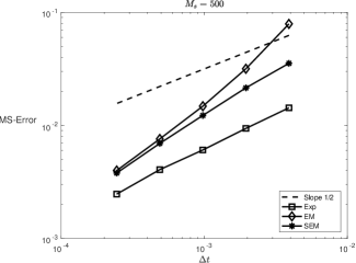
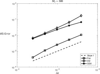
Figure 1: Strong rates of convergence for the stochastic Maxwell’s equation with $\mathbb{F}(\mathbb{U})=\mathbb{U}+\cos(\mathbb{U})$ and $\mathbb{G}(\mathbb{U})=\sin(\mathbb{U})$ (left) and $\mathbb{F}(\mathbb{U})=\mathbb{U}$ and $\mathbb{G}(\mathbb{U})=\mathbbm{1}^{T}$ (right).

5.2 Averaged energy and divergence

We now illustrate the geometric properties of the exponential integrator stated in Section 4. We consider the problem (4) with $\lambda_{1}=\lambda_{2}=0.5$, the time interval $[0,5]$, a step size $\Delta t=0.01$ and $M_{s}=25000$ samples to approximate the expectations. The numerical averaged energies and divergences are displayed in Figure 2. The trace formula for the energy of the stochastic exponential integrator, as stated in Proposition 4.1, is observed in this figure (left and middle plots). This is in contrast with the wrong behavior of the SEM scheme and the EM scheme, where explosion in the energy is observed for the EM scheme (left plot). In this figure (right plot), one can also observe the preservation of the averaged divergence of the magnetic field along the numerical solution given by the exponential integrator. This confirms the result of Proposition 4.2.

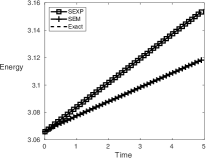
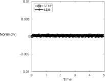
Figure 2: Averaged energy on a short time (left) and on a longer time (middle), averaged divergence (right).

References

• [1] R. Anton and D. Cohen, Exponential integrators for stochastic Schrödinger equations driven by Itô noise, special issue on SPDEs of J. Comput. Math. 36 (2018), no. 2, 276–309. MR 3771721
• [2] R. Anton, D. Cohen, S. Larsson, and X. Wang, Full discretization of semilinear stochastic wave equations driven by multiplicative noise, SIAM J. Numer. Anal. 54 (2016), no. 2, 1093–1119. MR 3484400
• [3] R. Anton, D. Cohen, and L. Quer-Sardanyons, A fully discrete approximation of the one-dimensional stochastic heat equation, IMA J. Numer. Anal. (2018).
• [4] P. Benner and J. Schneider, Uncertainty quantification for Maxwell’s equations using stochastic collocation and model order reduction, Int. J. Uncertain. Quantif. 5 (2015), no. 3, 195–208. MR 3390378
• [5] C. E. Bréhier, J. Cui, and J. Hong, Strong convergence rates of semi-discrete splitting approximations for stochastic Allen–Cahn equation, IMA J. Numer. Anal. (2018).
• [6] P. Brenner and V. Thomée, On rational approximations of semigroups, SIAM J. Numer. Anal. 16 (1979), no. 4, 683–694. MR 537280
• [7] E. Celledoni, D. Cohen, and B. Owren, Symmetric exponential integrators with an application to the cubic Schrödinger equation, Found. Comput. Math. 8 (2008), no. 3, 303–317. MR 2413146
• [8] C. Chen, J. Hong, and L. Ji, Mean-square convergence of a semi-discrete scheme for stochastic nonlinear Maxwell equations, arXiv:1802.10219 (2018).
• [9]  , Runge–Kutta semidiscretizations for stochastic Maxwell equations with additive noise, arXiv:1806.00922v1 (2018).
• [10] C. Chen, J. Hong, and L. Zhang, Preservation of physical properties of stochastic Maxwell equations with additive noise via stochastic multi-symplectic methods, J. Comput. Phys. 306 (2016), 500–519. MR 3432362
• [11] D. Cohen and G. Dujardin, Exponential integrators for nonlinear Schrödinger equations with white noise dispersion, Stoch. Partial Differ. Equ. Anal. Comput. 5 (2017), no. 4, 592–613. MR 3736655
• [12] D. Cohen and L. Gauckler, Exponential integrators for nonlinear Schrödinger equations over long times, BIT 52 (2012), no. 4, 877–903. MR 2995211
• [13] D. Cohen, S. Larsson, and M. Sigg, A trigonometric method for the linear stochastic wave equation, SIAM J. Numer. Anal. 51 (2013), no. 1, 204–222. MR 3033008
• [14] D. Cohen and L. Quer-Sardanyons, A fully discrete approximation of the one-dimensional stochastic wave equation, IMA J. Numer. Anal. 36 (2016), no. 1, 400–420. MR 3463447
• [15] J. Cui and J. Hong, Strong and weak convergence rates of finite element method for stochastic partial differential equation with non-globally lipschitz coefficients, arXiv:1806.01564 (2018).
• [16] J. Cui, J. Hong, Z. Liu, and W. Zhou, Stochastic symplectic and multi-symplectic methods for nonlinear Schrödinger equation with white noise dispersion, J. Comput. Phys. 342 (2017), 267–285. MR 3649275
• [17] M. Hochbruck, T. Jahnke, and R. Schnaubelt, Convergence of an ADI splitting for Maxwell’s equations, Numer. Math. 129 (2015), no. 3, 535–561. MR 3311460
• [18] M. Hochbruck, Ch. Lubich, and H. Selhofer, Exponential integrators for large systems of differential equations, SIAM J. Sci. Comput. 19 (1998), no. 5, 1552–1574. MR 1618808
• [19] M. Hochbruck and A. Ostermann, Exponential integrators, Acta Numer. 19 (2010), 209–286.
• [20] M. Hochbruck and T. Pažur, Implicit Runge-Kutta methods and discontinuous Galerkin discretizations for linear Maxwell’s equations, SIAM J. Numer. Anal. 53 (2015), no. 1, 485–507. MR 3313827
• [21] J. Hong, L. Ji, and L. Zhang, A stochastic multi-symplectic scheme for stochastic Maxwell equations with additive noise, J. Comput. Phys. 268 (2014), 255–268. MR 3192443
• [22] J. Hong, L. Ji, L. Zhang, and J. Cai, An energy-conserving method for stochastic Maxwell equations with multiplicative noise, J. Comput. Phys. 351 (2017), 216–229. MR 3713423
• [23] A. Jentzen and P. E. Kloeden, Overcoming the order barrier in the numerical approximation of stochastic partial differential equations with additive space-time noise, Proc. R. Soc. Lond. Ser. A Math. Phys. Eng. Sci. 465 (2009), no. 2102, 649–667. MR 2471778
• [24] Ch. Karle, J. Schweitzer, M. Hochbruck, and K. H. Spatschek, A parallel implementation of a two-dimensional fluid laser-plasma integrator for stratified plasma-vacuum systems, J. Comput. Phys. 227 (2008), no. 16, 7701–7719. MR 2437586
• [25] Y. Komori and K. Burrage, A stochastic exponential Euler scheme for simulation of stiff biochemical reaction systems, BIT 54 (2014), no. 4, 1067–1085. MR 3292538
• [26] Y. Komori, D. Cohen, and K. Burrage, Weak second order explicit exponential Runge–Kutta methods for stochastic differential equations, SIAM J. Sci. Comp 39 (2017), no. 6, A2857–A2878. MR 3735294
• [27] L. Kurt and T. Schäfer, Propagation of ultra-short solitons in stochastic Maxwell’s equations, J. Math. Phys. 55 (2014), no. 1, 011503, 11. MR 3390409
• [28] K. B. Liaskos, I. G. Stratis, and A. N. Yannacopoulos, Stochastic integrodifferential equations in Hilbert spaces with applications in electromagnetics, J. Integral Equations Appl. 22 (2010), no. 4, 559–590. MR 2755415
• [29] G. J. Lord and A. Tambue, Stochastic exponential integrators for the finite element discretization of SPDEs for multiplicative and additive noise, IMA J. Numer. Anal. 33 (2013), no. 2, 515–543. MR 3047942
• [30] P. Monk, Finite element methods for Maxwell’s equations, Numerical Mathematics and Scientific Computation, Oxford University Press, New York, 2003. MR 2059447
• [31] J. Niegemann, L. Tkeshelashvili, and K. Busch, Higher-order time-domain simulations of Maxwell’s equations using Krylov-subspace methods, Journal of Computational and Theoretical Nanoscience 4 (2007), no. 3, 627–634.
• [32] G. N. Ord, A stochastic model of Maxwell’s equations in $1+1$ dimensions, Internat. J. Theoret. Phys. 35 (1996), no. 2, 263–266. MR 1372172
• [33] T. Pažur, Error analysis of implicit and exponential time integration of linear maxwells equations, Ph.D. thesis, Karlsruhe Institute of Technology, 2013, Karlsruhe, KIT, Diss., 2013, p. 132.
• [34] R. Qi and X. Wang, An accelerated exponential time integrator for semi-linear stochastic strongly damped wave equation with additive noise, J. Math. Anal. Appl. 447 (2017), no. 2, 988–1008. MR 3573128
• [35] S. M. Rytov, Y. A. Kravtsov, and V. I. Tatarskiĭ, Principles of statistical radiophysics 3, Springer-Verlag, Berlin, 1989, Elements of random fields, Translated from the second Russian edition by Alexander P. Repyev. MR 1002949
• [36] C. Shi, Y. Xiao, and C. Zhang, The convergence and MS stability of exponential Euler method for semilinear stochastic differential equations, Abstr. Appl. Anal. (2012), Art. ID 350407, 19. MR 2965478
• [37] M. Tokman and P. M. Bellan, Three-dimensional model of the structure and evolution of coronal mass ejections, The Astrophysical Journal 567 (2002), no. 2, 1202.
• [38] J. G. Verwer, Component splitting for semi-discrete Maxwell equations, BIT 51 (2011), no. 2, 427–445. MR 2806538
• [39] J. G. Verwer and M. A. Botchev, Unconditionally stable integration of Maxwell’s equations, Linear Algebra Appl. 431 (2009), no. 3-4, 300–317. MR 2528933
• [40] X. Wang, An exponential integrator scheme for time discretization of nonlinear stochastic wave equation, J. Sci. Comput. 64 (2015), no. 1, 234–263. MR 3353942
• [41] K. Zhang, Numerical studies of some stochastic partial differential equations, Ph.D. thesis, The Chinese University of Hong Kong, 2008, Thesis (Ph.D.)–The Chinese University of Hong Kong (Hong Kong), p. 155. MR 2713292