Two-Hop Walks Indicate PageRank Order

Abstract

This paper shows that pairwise PageRank orders emerge from two-hop walks. The main tool used here refers to a specially designed sign-mirror function and a parameter curve, whose low-order derivative information implies pairwise PageRank orders with high probability. We study the pairwise correct rate by placing the Google matrix G in a probabilistic framework, where G may be equipped with different random ensembles for model-generated or real-world networks with sparse, small-world, scale-free features, the proof of which is mixed by mathematical and numerical evidence. We believe that the underlying spectral distribution of aforementioned networks is responsible for the high pairwise correct rate. Moreover, the perspective of this paper naturally leads to an $O(1)$ algorithm for any single pairwise PageRank comparison if assuming both $\textbf{A}=\textbf{G}-\textbf{I}_{n}$, where $\textbf{I}_{n}$ denotes the identity matrix of order $n$, and $\textbf{A}^{2}$ are ready on hand (e.g., constructed offline in an incremental manner), based on which it is easy to extract the top $k$ list in $O(kn)$, thus making it possible for PageRank algorithm to deal with super large-scale datasets in real time.

1 Introduction

The PageRank algorithm and related variants have attracted much attention in many applications of practical interests [1, 2, 3], especially known for their key role in the Google’s search engine. These principal eigenvector (the one corresponding to the largest eigenvalue) based algorithms share the same spirit and were rediscovered again and again by different communities from 1950’s. PageRank-type algorithms have appeared in the literatures on bibliometrics [4, 5, 6], sociometry [7, 8], econometrics [9], or web link analysis [10], etc. Two excellent historical reviews on this technique can be found in [11, 12].

Regardless of various motivations, this family of algorithms stand on the similar observations: an entity (person, page, node, etc) is important if it is pointed by other important entities, thus the resulting importance score should be computed in a recursive manner. More precisely, given a $n$-dimensional matrix G with its element $g_{ij}$ encoding some form of endorsement sent from the $j^{\text{th}}$ entity to the $i^{\text{th}}$ entity (both G and the transpose of G are alternately used in literatures, but which introduces no essential difference. Here, the former is adopted for convenience), then the importance score vector r is defined as the solution of the linear system:

$$\textbf{G}\textbf{r}=\textbf{r}.$$ (1)

However, some constraints are required for G such that there exists an unique and nonnegative solution in (1). In the PageRank algorithm, G is constructed by [10, 13]

$$\textbf{G}=\alpha(\widehat{\textbf{G}}+\textbf{ud}^{T})+(1-\alpha)\textbf{v}\textbf{1}^{T},$$ (2)

where $\widehat{\textbf{G}}$ is the column-normalized adjacent matrix of the web graph, i.e., the $(i,j)^{\text{th}}$ element of $\widehat{\textbf{G}}$ is one divided by the outdegree of the $j^{\text{th}}$ page if there is an link from the $j^{\text{th}}$ page to the $i^{\text{th}}$ page (zero otherwise), 1 is the all-ones vector, d is the indicator vector of dangling nodes (those having no outgoing edges), u and v are nonnegative and have unit $l_{1}$ norm (known as the dangling-node and personalization vectors, respectively. By default $\textbf{u}=\textbf{v}=\textbf{1}/n$), and $\alpha\in[0,1)$ is the damping factor (had better not be too close to 1. Usually $\alpha=0.85$ by default) for avoiding the “sink effect” caused by the modules with in- but no out-links [14]. Then, it is easy to verify that G constructed as above is a markov matrix with each column summing to one, and has an unrepeated largest eigenvalue valued 1 corresponding to the left eigenvector 1 (the modulus of the second largest eigenvalue of G is upper-bounded by $\alpha$ [15]). Due to the Perron$-$Frobenius theorem [9], this means that the (right) positive principal eigenvector of G actually is the unique PageRank vector in (1). Note that such a solution is only defined up to a positive scale, but introducing no harm in the ranking context.

1.1 Related Work

The humongous size of the World Wide Web and its fast growing rate make the evaluation of the PageRank vector one of the most demanding computational tasks ever, which causes the main obstacle of applying the PageRank algorithm to real-world applications since current principal eigenvector solvers for matrices of order over hundreds of thousands are still prohibitive in both and time and memory. Much effort for accelerating the PageRank algorithm has been carried out from different view, such as Monte Carlo method [16], random walk [17], power method or general linear system [18, 19], graph theory [20, 21, 22], Schrödinger equation [23], and quantum networks [24, 25]. More recent related advances on this topic can be found in [26, 27, 28, 29, 30, 31, 32, 33, 34, 35, 36]. However, it seems that one important fact is totally ignored when achieving speed-up: the exact value of the PagaRank vector is generally immaterial and what is really interesting is the ranking list, especially the top $k$ list in general. To the best of our knowledge, no research has been carried out on this way. The problem addressed in this paper will follow this direction for extracting the pairwise PageRank order in $O(1)$ using a very different insight if assuming both $\textbf{G}-\textbf{I}_{n}$ and $(\textbf{G}-\textbf{I}_{n})^{2}$ are ready in memory, based on which it is straightforward to obtain the top $k$ list in $O(kn)$. Our proposed algorithm avoids any effort of computing the exact value of the principle eigenvector of G.

1.2 Outline of Our Algorithm

In this paper, we always assume that G is a nonnegative real matrix with the spectral radius $1$, and 1 is an unique eigenvalue. We will use $\textbf{r}=[r_{1},\cdots,r_{n}]^{T}$ to denote arbitrary nonnegative principal eigenvector of G although the PageRank vector may be defined up to a positive scale. Let $\textbf{A}=\textbf{G}-\textbf{I}_{n}=(a_{ij})$, where $\textbf{I}_{n}$ is the unit matrix of order $n$. The main tool used in this paper is a specially designed curve $\textbf{F}(\textbf{A},\textbf{w},t)=[F_{1}(t)$, $\cdots$, $F_{n}(t)]\in\mathbb{R}^{n}$, where $\textbf{A},\textbf{w}$ and $t$ are three parameters. Here, we drop the dependency of $F_{k}(t)$ on A and w to make notations less cluttered. Throughout the paper, we will indicate vectors and matrices using bold faced letters.

We expect $\textbf{F}(\textbf{A},\textbf{w},t)$ to have the following properties: (a). For any positive w, the curve converges to the positive principal eigenvector of A (thus converges to r) as $t\rightarrow\infty$. Let $\Delta_{ij}(t)=F_{i}(t)-F_{j}(t)$, thus the task of comparing the PageRank score between the $i^{\text{th}}$ and $j^{\text{th}}$ nodes is reduced to determining the sign of $\Delta_{ij}(\infty)=F_{i}(\infty)-F_{j}(\infty)=r_{i}-r_{j}$; (b). Denote by $\textbf{F}^{(m)}(\textbf{A},\textbf{w},t)$ the $m^{\text{th}}$-order derivative of F w.r.t. $t$, which had better be a simple function of w and A such that evaluating it at $t=0$ causes relatively low computational cost; (c). Around the neighbourhood of $t=0$, the shape of $(F_{i}(t),F_{j}(t)),i\neq j,$ on the $\overline{x_{i}x_{j}}$ plane (spanned by the $i^{\text{th}}$ and $j^{\text{th}}$ axes in $\mathbb{R}^{n}$) can be flexibly controlled by w and $\textbf{F}^{(k)}(\textbf{A},\textbf{w},t),k=1,\cdots,m$.

With a carefully chosen w, it is possible to find a scale function $\phi_{ij}(\textbf{A},\textbf{w}$, $\textbf{F}^{(1)}(\textbf{A},\textbf{w},0),\!\cdots\!,\textbf{F}^{(m)}(\textbf{A},\textbf{w},0))$, simplified as $\phi_{ij}$, such that the probability $\pi_{ij}=\text{Pr}(\phi_{ij}\Delta_{ij}(\infty)>0)$ is sufficiently close to one. We call $\phi_{ij}$ the sign-mirror function for $\Delta_{ij}(\infty)$ since it reflects the sign of $\Delta_{ij}(\infty)$ in a probabilistic sense shown as above, although $\phi_{ij}$ itself only contains the local information of $\textbf{F}(\textbf{A},\textbf{w},t)$ around $t=0$. Furthermore, to avoid unnecessary computational cost, we also expect that small $m$ can do this job.

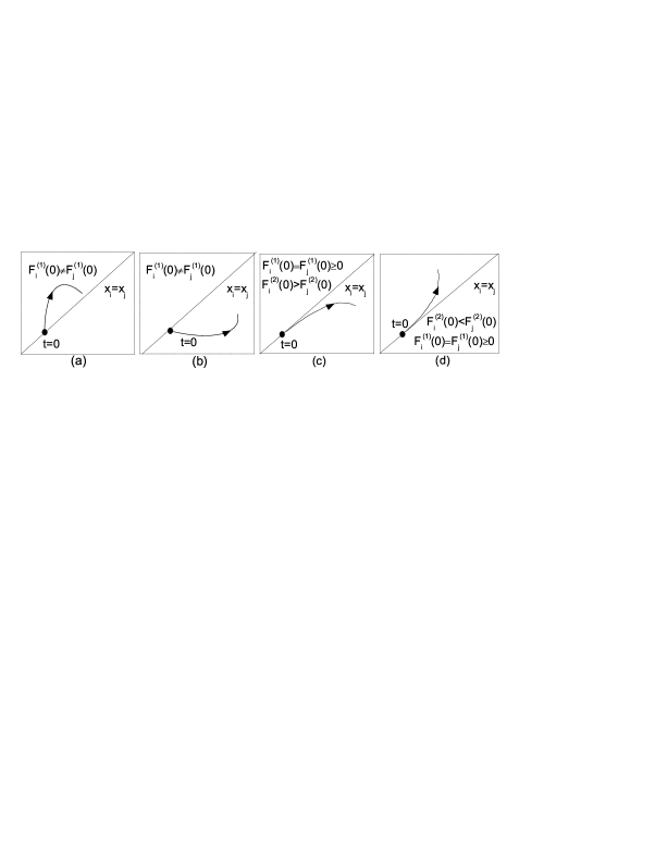
Figure 1: Four possible trajectories of $(F_{i}(t),F_{j}(t))$ on the $\overline{x_{i}x_{j}}$ plane with the $x_{i}$ and $x_{j}$ axes along horizontal and direction, respectively. In all the cases, w’s are picked out such that $(F_{i}(0),F_{j}(0))$’s locate on the line $x_{i}=x_{j}$. The last two are our desired cases, where both trajectories are tangent to $x_{i}=x_{j}$ with nonequal acceleration at $t=0$. Roughly speaking, this is due to the fact that in such cases we have more confidence to predict the sign of $F_{i}(\infty)-F_{j}(\infty)$ only based on $\textbf{A},\textbf{w}$, and $\textbf{F}^{(k)}(\textbf{A},\textbf{w},0),k=1,\cdots,m$.

Section 2 provides a curve equipped with the above properties with $m\geq 2$. There we also construct the corresponding sign-mirror function $\phi_{ij}$ and formulate $\pi_{ij}$ as a function of $\theta$, an angle variable dependent on the eigenvalue distribution of A. In the same section, we discuss some extensions of the algorithms. Section 3 checks the numerical properties of $\theta$, then verifies that $\pi_{ij}$ keeps small for variant types of model-generated or real-world graphs (sparse, scale-free, small-world, etc). This means that with a high probability the proposed algorithm succeeds to extract the true pairwise PageRank order for those common types of graphs mentioned as above. Then, it is relatively straightforward to develop a top $k$ list extraction algorithm based on partial (not total) pairwise orders, which will be discussed in section 4.

Nevertheless, it will be helpful to roughly imagine how such a curve possibly looks. Fig. 1 plots four possible trajectories of $(F_{i}(t),F_{j}(t))$ on the $\overline{x_{i}x_{j}}$ plane. Intuitively, $(F_{i}(t),F_{j}(t))$’s plotted in Fig. 1(a) and (b) are unpredictable in the sense that intuitively we have no confidence to predict whether they will cross the line $x_{i}=x_{j}$ at some $t>0$ or not. On the contrary, $(F_{i}(t),F_{j}(t))$’s shown in Fig. 1(c) or (d) seem more revealing due to the following facts: with higher probability, those two curves will not cross the line $x_{i}=x_{j}$ again for $t>0$ since both have been tangent to the line $x_{i}=x_{j}$ at $t=0$, and will locally move away from the line $x_{i}=x_{j}$ soon since they have unequal acceleration along axes at $t=0$. In fact, the imagined Fig. 1(c) and (d) do motivate us to construct an eligible sign-mirror function from a geometric view.

Finally, we point out that the algorithm of this paper is not only valid for the Google matrix defined in (2), which can even be applied to the non-markov matrix G as long as G meets the two conditions presented at the beginning of this subsection.

2 Model

Let $\text{i}=\sqrt{-1}$ be the imaginary unit and $\text{{diag}}[\textbf{A}_{1},\cdots,\textbf{A}_{s}]$ be a block diagonal matrix, where $\textbf{A}_{k},k=1,\cdots,s$, is a square matrix at the $i^{\text{th}}$ diagonal block. Unless specially mentioned, in this paper $\textbf{A}=\textbf{G}-\textbf{I}_{n}$ and G is defined at the beginning of subsection 1.2. From a practical view, we also assume that G (thus A) is diagonalizable since any matrix can be perturbed into a diagonalizable one with perturbation arbitrary small. Thus, A is real and diagonalizable, and all the eigenvalues of A except the unrepeated zero eigenvalue have negative real parts.

2.1 Designing Curve

Lemma 1. [37] For any real and diagonalizable matrix A of order $n$, there is an invertible matrix P such that

$$\textbf{A}=\textbf{P}\cdot\text{{diag}}[\underbrace{\lambda_{1},\cdots,\lambda_{r}}_{r},\underbrace{\textbf{A}_{r+1},\cdots,\textbf{A}_{r+s}}_{s}]\cdot\textbf{P}^{-1},\quad r+2s=n,\quad 0\leq r\leq n,$$ (3)

where

$$\ \textbf{P}=[\underbrace{\textbf{p}_{1}\ ,\ \ \cdots\ \ ,\ \textbf{p}_{r}}_{r\text{ real eigenvectors}},\underbrace{\textbf{p}_{\text{R},r+1},\textbf{p}_{\text{I},r+1},\cdots,\textbf{p}_{\text{R},r+s},\textbf{p}_{\text{I},r+s}}_{s\text{ pairs of complex eigenvectors}}],$$

$$\textbf{A}_{r+k}=\left(\begin{array}[]{cccccc}\lambda_{\text{R},r+k}&\lambda_{\text{I},r+k}\\ -\lambda_{\text{I},r+k}&\lambda_{\text{R},r+k}\end{array}\right),k=1,\cdots,s.\qquad\qquad$$

In the above equation, $\lambda_{k},k=1,\cdots,r,$ are $r$ real eigenvalues of A sorted in descending order, corresponding to the $r$ real eigenvectors $\textbf{p}_{k}$, and $\lambda_{\text{R},r+k}\pm\text{i}\lambda_{\text{I},r+k},k=1,\cdots,s$, are $s$ pairs of complex eigenvalues of A (sorted descendingly w.r.t. the real parts) corresponding to the $s$ pairs of complex eigenvectors $\textbf{p}_{\text{R},r+k}\pm\text{i}\textbf{p}_{\text{I},r+k}$, respectively.

In this paper, there exists $\lambda_{1}=0$, and all the other $\lambda_{k}$’s ($k=2,\!\cdots\!,r$) as well as $\lambda_{\text{R},k}$’s ($k=r+1$, $\!\cdots$, $r+s$) are negative. Moreover, we will use $\textbf{p}_{k}$ to denote the $k^{\text{th}}$ column of P in lemma 1 for convenience, i.e., $\textbf{P}=$ $[\textbf{p}_{1},$ $\!\cdots\!,\textbf{p}_{r},\textbf{p}_{\text{R},r+1}$, $\textbf{p}_{\text{I},r+1},\!\cdots\!,\textbf{p}_{\text{R},r+s},\textbf{p}_{\text{I},r+s}]\!=\![\textbf{p}_{1},\cdots,\textbf{p}_{n}]$. Since $\textbf{p}_{1},\!\cdots\!,\textbf{p}_{n},$ are linearly independent, any w takes the form as

$$\textbf{w}=\sum_{k=1}^{n}w_{k}\textbf{p}_{k}.$$ (4)

Let $\textbf{V}=[\textbf{v}_{1}^{T},\cdots,\textbf{v}_{n}^{T}]^{T}=\textbf{P}^{-1}$, and define for $k=1,\cdots,s,$

$$\textbf{B}_{r+k}\!=\!\textbf{p}_{r\!+\!2k-1}\textbf{v}_{r\!+\!2k\!-\!1}^{T}\!+\!\textbf{p}_{r\!+\!2k}\textbf{v}_{r\!+\!2k}^{T},\quad\textbf{C}_{r+k}\!=\!\textbf{p}_{r\!+\!2k\!-\!1}\textbf{v}_{r\!+\!2k}^{T}\!-\!\textbf{p}_{r\!+\!2k}\textbf{v}_{r\!+\!2k\!-\!1}^{T}.\quad$$

Then it is ready to construct the following curve with the desired properties given in subsection 1.2:

$$\textbf{F}(\textbf{A},\textbf{w},t)\!=\!\!\left({\sum_{k=1}^{r}\!e^{\lambda_{k}t}\textbf{p}_{k}\textbf{v}_{k}^{T}\!\!+\!\sum_{k=1}^{s}\!e^{\lambda_{\text{R},r\!+\!k}t}\left[{\cos(\lambda_{\text{I},r\!+\!k}t)\textbf{B}_{r\!+\!k}\!\!+\!\sin(\lambda_{\text{I},r\!+\!k}t)\textbf{C}_{r\!+\!k}}\right]}\right)\textbf{w},$$ (5)

where $t\geq 0$ is the time parameter and w is the $n$-dimensional “shape adjusting” vector. Although $\textbf{p}_{k}$ and $\textbf{v}_{k}$ appear in (5), it is not necessary to compute them throughout our algorithm, which will be clear in the sequel.

Lemma 2. There exist $\textbf{F}(\textbf{A},\textbf{w},0)=\textbf{w}$ and $\textbf{F}(\textbf{A},\textbf{w},\infty)=w_{1}\textbf{p}_{1}$, where $w_{1}$ is the projection of w on $\textbf{p}_{1}$.
Proof. Noting $\textbf{F}(\textbf{A},\textbf{w},0)=(\sum_{k=1}^{n}\textbf{p}_{k}\textbf{v}_{k}^{T})\textbf{w}$ and $\textbf{PV}=\textbf{I}_{n}$, thus the first equality holds. Since $\lambda_{1}=0$, $\lambda_{k}<0$ for $k=2,\cdots,r$, and $\lambda_{\text{R},r+k}$ for $k=1,\cdots,s$, there exists $\textbf{F}(\textbf{\emph{A}},\textbf{w},\infty)=\textbf{p}_{1}\textbf{v}_{1}^{T}\textbf{w}$. Due to $\textbf{VP}=\textbf{I}_{n}$, thus $\textbf{v}_{k}^{T}\textbf{p}_{k}=1$ and $\textbf{v}_{k}^{T}\textbf{p}_{h}=0$ for $\forall k\neq h$, which yields

$$\textbf{F}(\textbf{A},\textbf{w},\infty)=\textbf{p}_{1}\textbf{v}_{1}^{T}\sum_{k=1}^{n}w_{k}\textbf{p}_{k}=w_{1}\textbf{p}_{1}.$$

thus proving the second equality.

Clearly, $w_{1}\neq 0$ with probability 1, thus let us assume $w_{1}\neq 0$. In the sequel, we will also restrict w to be nonnegative, from which it is easy to see that $w_{1}\textbf{p}_{1}$ is always nonnegative, regardless of $\textbf{p}_{1}$ being the nonpositive or nonnegative principal eigenvector of G. Based on the above analysis and lemma 2, we can write $\textbf{F}(\textbf{A},\textbf{w},\infty)=\textbf{r}$, which verifies the property (a) presented in subsection 1.2. Thus, the task of comparing the PageRank score for the pair of $(i,j)^{\text{th}}$ pages is equivalent to determining the sign of $\Delta_{ij}(\infty)=F_{i}(\infty)-F_{j}(\infty)$.

The next lemma shows that both the first- and second-order derivatives of $\textbf{F}(\textbf{A},\textbf{w},t)$ have a neat relation w.r.t. A and w at $t=0$, which coincides with the highly desired property (b) given in subsection 1.2.

Lemma 3. There exist $\textbf{F}^{(1)}(\textbf{A},\textbf{w},0)=\textbf{A}\textbf{w}$ and $\textbf{F}^{(2)}(\textbf{A},\textbf{w},0)=\textbf{A}^{2}\textbf{w}$.
Proof. From (3), we have

A $$= \sum_{k=1}^{r}\lambda_{k}\textbf{p}_{k}\textbf{v}_{k}^{T}+\sum_{k=1}^{s}[(\lambda_{\text{R},r+k}\textbf{p}_{r+2k-1}\!-\!\lambda_{\text{I},r+k}\textbf{p}_{r+2k})\textbf{v}_{r+2k-1}^{T}$$ (6)

$$\qquad\qquad\quad\ +(\lambda_{\text{I},r+k}\textbf{p}_{r+2k-1}+\lambda_{\text{R},r+k}\textbf{p}_{r+2k})\textbf{v}_{r+2k}^{T}]$$

$$= \sum_{k=1}^{r}\lambda_{k}\textbf{p}_{k}\textbf{v}_{k}^{T}+\sum_{k=1}^{s}(\lambda_{\text{R},r+k}\textbf{B}_{r+k}+\lambda_{\text{I},r+k}\textbf{C}_{r+k}).$$

Similarly, from the equality $\textbf{A}^{2}\!=\!\textbf{P}\!\cdot\!\text{{diag}}[\lambda_{1}^{2},\!\cdots\!,\lambda_{r}^{2},\textbf{A}_{r+1}^{2},\!\cdots\!,\textbf{A}_{r+s}^{2}]\!\cdot\!\textbf{P}^{-1}$, a simple computation shows that

$$\textbf{A}^{2}=\sum_{k=1}^{r}\lambda_{k}^{2}\textbf{p}_{k}\textbf{v}_{k}^{T}+\sum_{k=1}^{s}[(\lambda_{\text{R},r+k}^{2}-\lambda_{\text{I},r+k}^{2})\textbf{B}_{r+k}+2\lambda_{\text{R},r+k}\lambda_{\text{I},r+k}\textbf{C}_{r+k})].$$ (7)

Based on the definition of $\textbf{F}(\textbf{A},\textbf{w},t)$ as in (5), a direct computation yields

$$\textbf{F}^{(1)}(\textbf{A},\textbf{w},0)\!=\!\frac{\text{d}\textbf{F}(\textbf{A},\textbf{w},t)}{\text{d}t}\left.\right|_{t=0}\!=\!\left({\sum_{k=1}^{r}\lambda_{k}\textbf{p}_{k}\textbf{v}_{k}^{T}+\sum_{k=1}^{s}\left({\lambda_{\text{R},r+k}\textbf{B}_{r+k}+\lambda_{\text{I},r+k}\textbf{C}_{r+k}}\right)}\right)\textbf{w}\overset{\text{(6)}}{=\!\!=}\textbf{Aw},$$

$$\textbf{F}^{(2)}(\textbf{A},\textbf{w},0)\!\!\!\!\! = \!\!\!\!\!\frac{\text{d}^{2}\textbf{F}(\textbf{A},\textbf{w},t)}{\text{d}t^{2}}\left.\right|_{t=0}$$

$$= \!\!\!\!\!\left({\sum_{k=1}^{r}\!\lambda_{k}^{2}\textbf{p}_{k}\textbf{v}_{k}^{T}\!+\!\sum_{k=1}^{s}\!\left({\lambda_{\text{R},r+k}^{2}\textbf{B}_{r+k}\!+\!2\lambda_{\text{R},r+k}\lambda_{\text{I},r+k}\textbf{C}_{r+k}\!-\!\lambda_{\text{I},r+k}^{2}\textbf{B}_{r+k}}\right)}\right)\!\textbf{w}\!\!\overset{\text{(7)}}{=\!\!=}\textbf{A}^{2}\textbf{w}.$$

thus proving the lemma.

2.2 Designing the Sign-Mirror Function

Let $\textbf{F}^{(m)}_{k}(\textbf{A},\textbf{w},0)$ and $(\textbf{A}^{m}\textbf{w})_{k},m=1,2,$ be the $k^{\text{th}}$ element of $\textbf{F}^{(m)}(\textbf{A},\textbf{w},0)$ and $\textbf{A}^{m}\textbf{w}$, respectively. In this subsection, we will focus on the key part of our eigenvector-computation-free algorithm: constructing the sign-mirror function $\phi_{ij}$ for $\Delta_{ij}(\infty)$ (recall the notations defined in subsection 1.2). Obviously, the bigger $\pi_{ij}$ is, with more confidence $\Delta_{ij}(\infty)$ and $\phi_{ij}$ share the same sign, In such a manner, we say that the sign of $\Delta_{ij}(\infty)$, which indicates the PageRank score order for the pair of the $(i,j)^{\text{th}}$ pages, is mirrored by the sign of $\phi_{ij}$. As mentioned before, Fig. 1 suggests an intuition for constructing the sign-mirror function as follows: Let $\phi_{ij}\!=\!\textbf{F}^{(2)}_{i}(\textbf{A},\textbf{w},0)\!-\!\textbf{F}^{(2)}_{j}(\textbf{A},\textbf{w},0)$, under the constraints $\textbf{F}^{(1)}_{i}(\textbf{A},\textbf{w},0)$ $=$ $\textbf{F}^{(1)}_{j}(\textbf{A},\textbf{w},0),\textbf{w}\geq 0$ and $w_{i}=w_{j}$. From lemma 3, the above equations can be rewritten into

$$\qquad\quad\phi_{ij}\!=\!(\textbf{A}^{2}\textbf{w})_{i}\!-\!(\textbf{A}^{2}\textbf{w})_{j},\quad\text{with}\quad w_{i}=w_{j},\ \textbf{w}\geq 0,\ (\textbf{A}\textbf{w})_{i}=(\textbf{A}\textbf{w})_{j},$$ (8)

which possibly is the simplest form for $\phi_{ij}$ to adapt in practice. Although other more sophisticated candidates may be considered, $\phi_{ij}$ constructed as above has worked well enough for our goal.

Note that there exit many choices for w meeting the constraints in (8). For reducing computational cost, in this paper we suggest to restrict w in the type of vectors only composed of three different values.

Let $\mathcal{J}\!\subsetneqq\!\{1,\!\cdots\!,n\}$ be an index subset containing $i$ and $j$ such that $\sum_{k\in\mathcal{J}}(a_{ik}\!-\!a_{jk})\!\neq\!0$. Clearly, $\mathcal{J}$ does not exist if and only if $a_{ii}+a_{ij}\!=\!a_{ji}+a_{jj}$ and $a_{ik}\!=\!a_{jk},\forall k\!\neq\!i,j$, which corresponds to an event with zero probability if regarding A as a random matrix. In what follows we assume the existence of $\mathcal{J}$.

Let $h\notin\mathcal{J}$ be any index such that $a_{ih}-a_{jh}$ has the opposite sign to that of $\sum\nolimits_{k\in\mathcal{J}}(a_{ik}-a_{jk})$ (the exceptional case where $h$ does not exist will be discussed later). Then, let $\zeta_{ij}=\sum\nolimits_{k\notin\{h\}\cup\mathcal{J}}(a_{jk}-a_{ik})$ and define w by

$$w_{k}\!\!=\!\!\frac{-q(a_{ih}\!\!-\!a_{jh})\!-\!\zeta_{ij}}{\sum\nolimits_{k\in\mathcal{J}}(a_{ik}\!-\!a_{jk})}\!\!\triangleq\!z,\forall k\!\in\!\mathcal{J};\ w_{h}\!\!=\!\varepsilon\!+\!\max(0,\!\!\frac{\zeta_{ij}}{a_{ih}\!\!-\!\!a_{jh}})\!\!\triangleq\!\!q;\ \text{ otherwise }w_{k}\!\!=\!\!1.$$ (9)

where $\varepsilon$ is an adjustable positive constant ($\varepsilon=10^{-5}$ is used in our simulation). It is easy to verify that w constructed as above meets all the constraints in (8). Let $b_{ij}$ be the $(i,j)^{\text{th}}$ element of $\textbf{B}=\textbf{A}^{2}=(b_{ij})$. A simple simplification shows that with w as in (9) $\phi_{ij}$ can be rewritten into:

$$\phi_{ij}=z\sum\nolimits_{k\in\mathcal{J}}(b_{ik}-b_{jk})+q(b_{ih}-b_{jh})+\sum\nolimits_{k\notin\mathcal{J}\cup\{h\}}(b_{ik}-b_{jk}).$$

Specially, in the case of $\mathcal{J}=\{i,j\}$, i.e., $a_{ii}+a_{ij}\neq a_{ji}+a_{jj}$, which corresponds to an almost sure event in practice, let us denote by $\text{sum}_{k}(\textbf{A})$ and $\text{sum}_{k}(\textbf{B})$ the sum of the $k^{\text{th}}$ row of A and B, respectively. In this case, $\phi_{ij}$ takes a more computation-friendly form:

$$\phi_{ij}=\text{sum}_{i}(\textbf{B})-\text{sum}_{j}(\textbf{B})+(z-1)(b_{ii}+b_{ij}-b_{ji}-b_{jj})+(q-1)(b_{ih}-b_{jh}),$$ (10)

where $q$ and $z=\frac{\text{sum}_{j}(\textbf{A})-\text{sum}_{i}(\textbf{A})+(1-q)(a_{ih}-a_{jh})}{a_{ii}+a_{ij}-a_{ji}-a_{jj}}+1$ are computed from (9) with $\mathcal{J}=\{i,j\}$. Now, we conclude our pairwise PageRank ranking algorithm as follows:

$$\phi_{ij}>0\ \Rightarrow\ r_{i}>r_{j}\qquad\text{ or }\qquad\phi_{ij}<0\ \Rightarrow\ r_{i}<r_{j}.$$ (11)

The whole algorithm flow is depicted in Algorithm 1. As for the exceptional case that no index $h$ exists, i.e., $a_{ik}\!-\!a_{jk},k\!\neq\!i,j,$ are all positive (or negative), which is an almost null event in practice, it is intuitive to claim $r_{i}\!>\!r_{j}$ (or $r_{i}\!<\!r_{j}$) due to the PageRank principle.

Input: $\text{{A}}=\text{{G}}-\text{{I}}_{n}$ and its square B, where G is constructed as (2).

1 Randomly choose $\mathcal{J}$ satisfying $i,j\in\mathcal{J}\!\subsetneqq\!\{1,\!\cdots\!,n\},\sum_{k\in\mathcal{J}}(a_{ik}\!-\!a_{jk})\!\neq\!0$.

2 Randomly choose $h\notin\mathcal{J}$ satisfying $(a_{ih}-a_{jh})\sum\nolimits_{k\in\mathcal{J}}(a_{ik}-a_{jk})<0$.

3 Compute $\phi_{ij}=z\sum\nolimits_{k\in\mathcal{J}}(b_{ik}-b_{jk})+q(b_{ih}-b_{jh})+\sum\nolimits_{k\notin\mathcal{J}\cup\{h\}}(b_{ik}-b_{jk})$, with $z$ and $q$ defined in (9).

Output: $\phi_{ij}>0\ \Rightarrow\ r_{i}>r_{j}\text{ or }\phi_{ij}<0\ \Rightarrow\ r_{i}<r_{j}$, where $r_{i}$ and $r_{j}$ are the estimated PageRank score of nodes $i$ and $j$.

Algorithm 1 Comparing the PageRank score between nodes $i$ and $j$.

Finally, we provide a complexity analysis for single run of (11). If A and $\textbf{B}=\textbf{A}^{2}$ (constructed offline) are ready in memory, the time cost comes from two parts: time for finding the index $h$ plus a dozen of simple algebraic computation involved in (9) and (10). Given $\sum\nolimits_{k\in\!\mathcal{J}}(a_{ik}\!\!-\!a_{jk})$, let $p$ be the probability that $a_{ih}\!\!-\!\!a_{jh}$ has the same sign as that of $\sum\nolimits_{k\in\!\mathcal{J}}(a_{ik}\!-\!a_{jk}\!)$ for a randomly chosen $h\!\notin\!\!\mathcal{J}$. Then, the mean number of sampling $h$ equals to $\lim\!_{n\!\rightarrow\infty}\!\sum\!_{k\!=\!1}^{n}k(1\!-\!p)p^{k-\!1}\!=\!\frac{1}{(1\!-\!p)^{2}}$, just a small constant. Thus, the time complexity for single run of (11) is $O(1)$. Moreover, it is easy to see that both A and B can be constructed incrementally. Actually, the whole algorithm (11) is almost ready to work in an incremental fashion with slight modifications, which is omitted here.

2.3 Evaluating $\pi_{ij}\quad$

Here, we study the probability $\pi_{ij}\!=\!\text{Pr}(\phi_{ij}\Delta_{ij}(\infty)\!>\!0)$ (recall the notations defined in subsection 1.2) given $\phi_{ij}$ constructed in (8), which determines the correct rate of our algorithm (11). Let $\textbf{p}_{k}\!=\![p_{1k},\cdots,p_{nk}]^{T},k\!=\!1,\cdots,n$, and $\tau_{k}^{ij}\!=\!p_{ik}-p_{jk}$, thus $\Delta_{ij}(\infty)=w_{1}\tau_{1}^{ij}$ from the second equality in lemma 2. Based on (4), the constraint $w_{i}\!=\!w_{j}$ in (8) means $\sum_{k=1}^{n}w_{k}\tau_{k}^{ij}=0$, i.e.,

$$\Delta_{ij}(\infty)=w_{1}\tau_{1}^{ij}=-\sum_{k=2}^{n}w_{k}\tau_{k}^{ij}.$$ (12)

Based on (4) and (6), the constraint $(\textbf{A}\textbf{w})_{i}=(\textbf{A}\textbf{w})_{j}$ in (8) indicates

$$0 = \sum_{k=2}^{r}\lambda_{k}w_{k}\tau_{k}^{ij}\!+\!\sum_{k=1}^{s}[\lambda_{\text{R},r+k}(w_{r+2k-1}\tau_{r+2k-1}^{ij}\!+\!w_{r+2k}\tau_{r+2k}^{ij})$$ (13)

$$+\lambda_{\text{I},r+k}(w_{r+2k}\tau_{r+2k-1}^{ij}\!-\!w_{r+2k-1}\tau_{r+2k}^{ij})].$$

where we use the fact $\lambda_{1}=0$, $\textbf{v}_{k}^{T}\textbf{p}_{k}=1$ and $\textbf{v}_{k}^{T}\textbf{p}_{h}=0$ for $\forall k\neq h$. Similarly, using (4) and (7), $\phi_{ij}=(\textbf{A}^{2}\textbf{w})_{i}-(\textbf{A}^{2}\textbf{w})_{j}$ can be rewritten into

$$\ \phi_{ij}=\!\!\!\!\!\!\!\!\!\! \sum_{k=2}^{r}\lambda_{k}^{2}w_{k}\tau_{k}^{ij}+\sum_{k=1}^{s}[(\lambda_{\text{R},r+k}^{2}\!-\!\lambda_{\text{I},r+k}^{2})(w_{r+2k-1}\tau_{r+2k-1}^{ij}\!+\!w_{r+2k}\tau_{r+2k}^{ij})$$ (14)

$$+\ 2\lambda_{\text{R},r+k}\lambda_{\text{I},r+k}(w_{r+2k}\tau_{r+2k-1}^{ij}\!-\!w_{r+2k-1}\tau_{r+2k}^{ij})].$$

Next, we want to eliminate one redundant item from both (12) and (14) with the help of (13). This redundant item corresponds to $(w_{r+1}\tau_{r+1}^{ij}\!+\!w_{r+2}\tau_{r+2}^{ij})$ if there exists $\lambda_{\text{R},r+1}$ (i.e, there are at least one pair of complex eigenvalues, called case 1), or to $w_{2}\tau_{2}^{ij}$ if there exists $\lambda_{2}$ (i.e, there are two or more real eigenvalues, called case 2). A direct computation gives the following theorem:

Theorem 4. Given any pair of $(i,j)$, we have $\phi_{ij}\Delta_{ij}(\infty)=(\widehat{\mbox{\boldmath{$\lambda$}}}_{1}^{T}\mbox{\boldmath{$\beta$}}^{ij})(\widehat{\mbox{\boldmath{$\lambda$}}}_{2}^{T}\mbox{\boldmath{$\beta$}}^{ij})$. In case 1, there exists

$$\mbox{\boldmath{$\beta$}}^{ij}\!\!=\![\underbrace{w_{2}\tau_{2}^{ij},\ \cdots,\ w_{r}\tau_{r}^{ij}}_{r-1},\ \underbrace{\gamma^{ij}_{r\!+\!2},\ \cdots,\ \gamma^{ij}_{r\!+\!2s}}_{2s-1}]^{T}\in\mathbb{R}^{n-2},$$

$$\overline{\mbox{\boldmath{$\lambda$}}}_{1}\!\!=\![\underbrace{\frac{\lambda_{2}}{\lambda_{\text{R},r\!+\!1}}\!-\!1,\!\cdots\!,\frac{\lambda_{r}}{\lambda_{\text{R},r\!+\!1}}\!-\!1}_{r-1},\underbrace{\frac{\lambda_{\text{I},r\!+\!1}}{\lambda_{\text{R},r\!+\!1}},\frac{\lambda_{\text{R},r\!+\!2}}{\lambda_{\text{R},r\!+\!1}}\!-\!1,\frac{\lambda_{\text{I},r\!+\!2}}{\lambda_{\text{R},r\!+\!1}},\!\cdots\!,\frac{\lambda_{\text{R},r\!+\!s}}{\lambda_{\text{R},r\!+\!1}}\!-\!1,\frac{\lambda_{\text{I},r\!+\!s}}{\lambda_{\text{R},r\!+\!1}}}_{2s-1}]^{T}\!\in\!\mathbb{R}^{n\!-\!2},$$

$$\overline{\mbox{\boldmath{$\lambda$}}}_{2}\!=\![\underbrace{d_{2},\!\cdots\!,d_{r}}_{r-1},\underbrace{e_{r\!+\!1}\!-\!c\lambda_{\text{I},r\!+\!1},f_{r\!+\!2}\!-\!c\lambda_{\text{R},r\!+\!2},e_{r\!+\!2}\!-\!c\lambda_{\text{I},r\!+\!2},\!\cdots\!,f_{r\!+\!s}\!-\!c\lambda_{\text{R},r\!+\!s},e_{r\!+\!s}\!-\!c\lambda_{\text{I},r\!+\!s}}_{2s-1}]^{T}\!\in\!\mathbb{R}^{n\!-\!2},\qquad\quad$$ (15)

where $\gamma^{ij}_{r\!+\!2k\!-\!1}\!=\!w_{r\!+\!2k\!-\!1}\tau_{r\!+\!2k\!-\!1}^{ij}+w_{r\!+\!2k}\tau_{r\!+\!2k}^{ij},\ \gamma^{ij}_{r\!+\!2k}\!=\!w_{r\!+\!2k}\tau_{r\!+\!2k\!-\!1}^{ij}\!-w_{r\!+\!2k\!-\!1}\tau_{r\!+\!2k}^{ij},k\!=\!1,\!\cdots\!,s,\ c\!=\!(\lambda_{\text{R},r\!+\!1}^{2}\!-\!\lambda_{\text{I},r\!+\!1}^{2})/\lambda_{\text{R},r\!+\!1}$, $d_{k}\!=\!\lambda_{k}(\lambda_{k}\!-\!c)$ for $k\!=\!2,\!\cdots\!,r$, $\ e_{r+k}\!=\!2\lambda_{\text{R},r\!+\!k}\lambda_{\text{I},r\!+\!k}$ for $k\!=\!1,\!\cdots\!,s$, and $f_{r\!+\!k}\!=\!\lambda_{\text{R},r\!+\!k}^{2}\!-\!\lambda_{\text{I},r\!+\!k}^{2}$ for $k\!=\!1,\!\cdots\!,s$.

In case 2, there exists

$$\qquad\quad\mbox{\boldmath{$\beta$}}^{ij}\!\! = \![\underbrace{w_{3}\tau_{3}^{ij},\!\cdots\!,w_{r}\tau_{r}^{ij}}_{r-2},\underbrace{\gamma^{ij}_{r\!+\!1},\!\cdots\!,\gamma^{ij}_{r\!+\!2s}}_{2s}]^{T}\!\in\!\mathbb{R}^{n-2},$$

$$\overline{\mbox{\boldmath{$\lambda$}}}_{1}\!\! = \![\underbrace{\frac{\lambda_{3}}{\lambda_{2}}\!-\!1,\cdots,\frac{\lambda_{r}}{\lambda_{2}}\!-\!1}_{r-2},\underbrace{\frac{\lambda_{\text{R},r\!+\!1}}{\lambda_{2}}\!-\!1,\frac{\lambda_{\text{I},r\!+\!1}}{\lambda_{2}},\frac{\lambda_{\text{R},r\!+\!2}}{\lambda_{2}}\!-\!1,\!\cdots\!,\frac{\lambda_{\text{R},r\!+\!s}}{\lambda_{2}}\!-\!1,\frac{\lambda_{\text{I},r\!+\!s}}{\lambda_{2}}}_{2s}]^{T}\!\in\!\mathbb{R}^{n\!-\!2},$$

$$\overline{\mbox{\boldmath{$\lambda$}}}_{2}\!\!\! = \!\!\!\!\!\![\underbrace{d_{3},\!\cdots\!\!,d_{r}}_{r-2},\underbrace{f_{r\!+\!1}\!-\!c\lambda_{\text{R},r\!+\!1},e_{r\!+\!1}\!-\!c\lambda_{\text{I},r\!+\!1},f_{r\!+\!2}\!-\!c\lambda_{\text{R},r\!+\!2},\!\cdots\!\!,f_{r\!+\!s}\!-\!c\lambda_{\text{R},r\!+\!s},e_{r\!+\!s}\!-\!c\lambda_{\text{I},r\!+\!s}}_{2s}]^{T}\!\!\!\in\!\mathbb{R}^{n\!-\!2},$$

Here, all variables are same to those in (15) except $c=\lambda_{2}$.

It is worthy noting that $\overline{\mbox{\boldmath{$\lambda$}}}_{1}$ and $\overline{\mbox{\boldmath{$\lambda$}}}_{2}$ are two ($n-2$)-dimensional random vectors only dependent on the eigenvalue distribution of $\textbf{A}=\textbf{G}-\textbf{I}_{n}$, and $\mbox{\boldmath{$\beta$}}^{ij}$ is a ($n-2$)-dimensional random vector w.r.t. the eigenvector distribution of A and the projections of w along eigenvectors. From now on, will treat the Google matrix G as a random one that encodes the topological structure of a model-generated or real-world networks following different ensembles, e.g., scale-free [38], or small-world [39], etc.

Denote by $\theta$ the angle between $\overline{\mbox{\boldmath{$\lambda$}}}_{1}$ and $\overline{\mbox{\boldmath{$\lambda$}}}_{2}$. The above theorem provides a geometric interpretation for $\pi_{ij}$. Imagining the bounded subspace in $\mathbb{R}^{n-2}$ where $\mbox{\boldmath{$\beta$}}_{ij}$ lives, as depicted in Fig. 2, theorem 4 shows that the event $\phi_{ij}\Delta_{ij}(\infty)\leq 0$ corresponds to two dark spherical wedges enclosed by the two $(n-2)$-dimensional hyperplanes $V_{1}$ and $V_{2}$ whose normal vectors are $\widehat{\mbox{\boldmath{$\lambda$}}}_{1}$ and $\widehat{\mbox{\boldmath{$\lambda$}}}_{2}$, respectively. Hence, in principle we can write $\pi_{ij}=1-\text{Vol}(dark)/\text{Vol}(all)$, where $\text{Vol}(dark)$ and $\text{Vol}(all)$ denote the weighted volumes of two dark wedges and the total subspace, respectively. Here, the volume is weighted by the probability density function of $\mbox{\boldmath{$\beta$}}_{ij}$, denoted by $\rho$. In general, it is impossible to obtain the analytical form of $\rho$ for the purpose of evaluating $\pi_{ij}$, but it is interesting to note that when $\theta\rightarrow 0$, there approximately exists $\pi_{ij}\rightarrow 1$, regardless of the exact form of $\rho$ and the direction of $\widehat{\mbox{\boldmath{$\lambda$}}}_{k},k=1,2$. Note that in this claim we use an intuitive assumption that the support of $\rho$ is not extremely concentrated around any low-dimensional hyperplane, which seems true from a practical view and will be discussed more later.

Figure 2: Two dark spherical wedges correspond to the event $\phi_{ij}\Delta_{ij}(\infty)\leq 0$, meaning that $\pi_{ij}=1-\frac{\theta}{180^{{}^{\circ}}}$.

The above analysis also explains why we try eliminating an redundant item from $\Delta_{ij}(\infty)$ and $\phi_{ij}$. The reason is that the resulting $\theta$ in such a manner would be close to a small angle as $n\rightarrow\infty$ (e.g., $n>1000$, in what follows $n$ is always assumed to be large enough unless specially stated) for a variant types of common networks, which will be detailedly verified in the next section.

Nevertheless, let us first look at some special cases to reveal the hidden motivation. To this end, let us consider the following types of undirected graphs as examples: 1). $\overline{\textbf{G}}\leftarrow\text{abs}(\text{rand}(n))$ or $\text{abs}(\text{randn}(n))$, followed by $\overline{\textbf{G}}\leftarrow\overline{\textbf{G}}+\overline{\textbf{G}}^{\prime}$ or $\overline{\textbf{G}}*\overline{\textbf{G}}^{\prime}$, where “randn($\cdot$)” and “rand($\cdot$)” are the functions, respectively for generating matrices whose elements follow the standard normal $\mathcal{N}(0,1)$ and uniform distribution in [0,1], and “abs($\cdot$)” denote the absolute value function in Matlab; 2). $\overline{\textbf{G}}$ is the adjacent matrix for an Erdös-Reényi (ER) graph [40]. We normalize each column of $\overline{\textbf{G}}$ to get $\widehat{\textbf{G}}$, then obtain G following (2) with default parameters.

In such a way, although G is generally asymmetric, $||\textbf{G}-\textbf{G}^{\prime}||$ is very small with high probability since the sums of each column of $\overline{\textbf{G}}$ are equal with high probability (thus $\widehat{\textbf{G}}$ is almost a constant scale of $\overline{\textbf{G}}$), meaning that G is “asymptotically symmetric”, i.e., all the eigenvalues of G are real with high probability. Surprisingly, in all of our experiments based on the above graphs generated by different $n$ (We also varied the sparse density for ER graphs), no complex eigenvalue appears at all! (however, it has been proven in [41] that for matrices with the elements following the standard normal distribution, the number of real eigenvalues scales with $\sqrt{n}$, instead of $n$). In a word, all the eigenvalues in these example typically are real, corresponding to the case 2 in theorem 4, and $\overline{\mbox{\boldmath{$\lambda$}}}_{k},k=1,2,$ will now take a more clean form as

$$\overline{\mbox{\boldmath{$\lambda$}}}_{1}=[\lambda_{3}-\lambda_{2},\!\cdots\!,\lambda_{n}-\lambda_{2}]^{T}/\lambda_{2},\quad\overline{\mbox{\boldmath{$\lambda$}}}_{2}=[\lambda_{3}(\lambda_{3}-\lambda_{2}),\!\cdots\!,\lambda_{n}(\lambda_{n}-\lambda_{2})]^{T},$$

$$\mbox{\boldmath{$\beta$}}^{ij}=[w_{3}\tau_{3}^{ij},\cdots,w_{n}\tau_{n}^{ij}]^{T}.\qquad\qquad\qquad\qquad\qquad$$ (16)

At first glance, if assuming all the eigenvalues are equally spaced on the real line (however, it is not true in general), a direct computation shows $\theta\!\rightarrow\!\arccos(\sqrt{15}/4)\!=\!14.74^{\circ}$. In fact, smaller $\theta$ may be expected. Note that the diagonal elements of G in these examples should have the same expectation, so should the off-diagonal elements. Therefore, the Theorem 1 in [42] or Theorem 1.1 in [43] can be applied here, which says that the gap between $\lambda_{1}$ and $\lambda_{2}$ is $O(n)$, and that between $\lambda_{i}$ and $\lambda_{i+1},i\geq 2,$ is only $O(\sqrt{n})$. Such unbalanced gap distribution was also observed in [44, 45] (e.g., refer to Fig. 1 in [44]) for Google matrices constructed from the Albert-Barabási model [38] or randomized real-world University networks [46]. Based on the above analysis, roughly speaking, there are $O(\sqrt{n})$ eigenvalues $\lambda_{k}$ satisfying $\lambda_{k}/\lambda_{3}\rightarrow 1$, meaning from (16) that the first $O(\sqrt{n})$ coordinates of $\overline{\mbox{\boldmath{$\lambda$}}}_{1}$ and $\overline{\mbox{\boldmath{$\lambda$}}}_{2}$ tend to be “collinear”. It is such an intrinsic “collinear effect” that forces $\theta$ close to zero.

Table. 1 depicts the mean and variance of $\theta$ in aforementioned examples over 800 sequential runs for each case, from which we see that in all the cases $\theta$ is concentrated around $0^{\circ}$ while the variance approaches to zero as $n$ increases. Generally, if assuming that $\rho$ is approximately constant along arbitrary direction in $\mathbb{R}^{n-2}$, there exists

$$\pi_{ij}\approx 1-\frac{\theta}{180^{\circ}}.$$ (17)

We will show in the next section that the above formula is highly agrees with our experimental results especially for large $n$, even although $\theta$ is not so close to 0 (as shown in the next section, typically $\theta$ is a small angle less than $10^{\circ}$ in most cases).

Table 1: Mean and variance of the angle between $\overline{\mbox{\boldmath{$\lambda$}}}_{1}$ and $\overline{\mbox{\boldmath{$\lambda$}}}_{2}$ in (16) averaged over 800 runs. Here, the Google matrix G is constructed as (2) with default parameters, where $\widehat{\textbf{G}}$ is the column-normalized version of $\overline{\textbf{G}}$ corresponding to six types of graphs T_k. T₁ (or T₂) corresponds to $\overline{\textbf{G}}\leftarrow$ $\text{abs}(\text{rand}(n))$ followed by $\overline{\textbf{G}}\leftarrow\overline{\textbf{G}}+\overline{\textbf{G}}^{\prime}$ (or $\overline{\textbf{G}}*\overline{\textbf{G}}^{\prime}$). T₃ (or T₄) is generated similarly to T₁ (or T₂), but with “rand(n)” replaced by “randn(n)”. T₅ and T₆ correspond to ER graphs with the sparse density valued at $0.1$ and $0.2$, respectively.

	$n=100$						$n=1000$						$n=2000$
	$\text{T}_{1}$	$\text{T}_{2}$	$\text{T}_{3}$	$\text{T}_{4}$	$\text{T}_{5}$	$\text{T}_{6}$	$\text{T}_{1}$	$\text{T}_{2}$	$\text{T}_{3}$	$\text{T}_{4}$	$\text{T}_{5}$	$\text{T}_{6}$	$\text{T}_{1}$	$\text{T}_{2}$	$\text{T}_{3}$	$\text{T}_{4}$	$\text{T}_{5}$	$\text{T}_{6}$
E$(\theta)$	1.42∘	0.16∘	1.84∘	0.15∘	8.51∘	6.17∘	0.46∘	0.09∘	0.6∘	0.01∘	3.22∘	2.19∘	0.32∘	0.04∘	0.43∘	0.008∘	2.33∘	1.57∘
Var$(\theta)$	$10^{-\!4}$	$10^{-\!6}$	$10^{-\!3}$	$10^{-\!5}$	$10^{-\!2}$	$10^{-\!3}$	$10^{-\!6}$	$10^{-\!9}$	$10^{-\!6}$	$10^{-\!8}$	$10^{-\!4}$	$10^{-\!5}$	$10^{-\!8}$	$10^{-\!10}$	$10^{-\!7}$	$10^{-\!10}$	$10^{-\!6}$	$10^{-\!6}$

2.4 Higher-Order Sign-Mirror Functions

Motivated by the $\phi_{ij}$ constructed in (8), it is natural to consider its higher-order version: $\phi_{ij}=(\textbf{A}^{m}\textbf{w})_{i}-(\textbf{A}^{m}\textbf{w})_{j}$, satisfying

$$w_{i}\!=\!w_{j},\ \textbf{w}\!\geq\!0,\quad(\textbf{A}^{k}\textbf{w})_{i}\!\!=\!\!(\textbf{A}^{k}\textbf{w})_{j},\ k\!\!=\!\!1,\cdots,m\!-\!1,$$ (18)

where $m$ is a preassigned positive integer. However, the practical algorithm in form keeps unchanged as (11).

To study $\pi_{ij}$ in this case, similar to what we do previously for the case of $m\!=\!2$, we first expand $\textbf{A}^{k}\textbf{w}$, $k\!=\!1,\!\cdots\!,m,$ using (3) and (4). Then, from the constraint $(\textbf{A}^{k}\textbf{w})_{i}\!=\!(\textbf{A}^{k}\textbf{w})_{j},k\!=\!1,\!\cdots\!,m\!-\!1,$ we obtain $m\!-\!1$ linear equations w.r.t. $w_{2}\tau_{2}^{ij},\cdots,$ $w_{r}\tau_{r}^{ij},\gamma^{ij}_{r+1},\cdots,\gamma^{ij}_{r+2s}$, thus we can represent $w_{2}\tau_{2}^{ij},\cdots,w_{m}\tau_{m}^{ij}$ using the linear combination of $w_{m+1}\tau_{m+1}^{ij},\cdots,w_{r}\tau_{r}^{ij},\gamma^{ij}_{r+1},\cdots,\gamma^{ij}_{r+2s}$ (here, without loss of generality we assume $\lambda_{m}\geq\lambda_{\text{R},r+1}$). Next, let us eliminate $w_{2}\tau_{2}^{ij},\cdots$, $w_{m}\tau_{m}^{ij}$, from the expressions of $\Delta_{ij}(\infty)$ in (12) and $\phi_{ij}=(\textbf{A}^{m}\textbf{w})_{i}\!-\!(\textbf{A}^{m}\textbf{w})_{j}$ in (18), finally leading to a tight form $\phi_{ij}\Delta_{ij}(\infty)=(\widehat{\mbox{\boldmath{$\lambda$}}}_{1}^{T}\mbox{\boldmath{$\beta$}}^{ij})(\widehat{\mbox{\boldmath{$\lambda$}}}_{2}^{T}\mbox{\boldmath{$\beta$}}^{ij})$ which formally is the same to that in theorem 4. However, $\widehat{\mbox{\boldmath{$\lambda$}}}_{k},k=1,2,$ and $\mbox{\boldmath{$\beta$}}^{ij}$ are of order $n-m$ in this case, and $\widehat{\mbox{\boldmath{$\lambda$}}}_{k}$ takes a more complex dependence on the eigenvalues. The biggest benefit own to higher-order sign-mirror functions lies in our numerical observations, as shown in Table. 2, that $\theta$ gets closer to zero as $m$ increases, which we believe is due to the stronger“collinear effect” between $\widehat{\mbox{\boldmath{$\lambda$}}}_{1}$ and $\widehat{\mbox{\boldmath{$\lambda$}}}_{2}$ for bigger $m$. However, this benefit is at the expense of more computational cost since up to $m$-order power of A is required. Moreover, to ensure the existence of w meeting the constraints in (18), there should be at least $m-1$ free variables in w (generally, the constraint $\textbf{w}\geq 0$ requires a few additional free variables involved in w), which is different from the case of $m=2$ where w can be composed of three different values as shown in (9).

Table 2: Mean and variance of $\theta$ based on higher-order sign-mirror functions with $m=3,4,$ averaged over 500 runs in each case, where T₅ and T₆ are the same graph ensembles used in Table. 1.

	$n\!=\!100,m\!=\!3$		$n\!=\!100,m\!=\!4$		$n\!=\!1000,m\!=\!3$		$n\!=\!1000,m\!=\!4$		$n\!=\!2000,m\!=\!3$		$n\!=\!2000,m\!=\!4$
	$\text{T}_{5}$	$\text{T}_{6}$	$\text{T}_{5}$	$\text{T}_{6}$	$\text{T}_{5}$	$\text{T}_{6}$	$\text{T}_{5}$	$\text{T}_{6}$	$\text{T}_{5}$	$\text{T}_{6}$	$\text{T}_{5}$	$\text{T}_{6}$
E$(\theta)$	5.97∘	4.46∘	4.61∘	3.48∘	2.42∘	1.68∘	1.93∘	1.34∘	1.76∘	1.20∘	1.41∘	0.97∘
Var$(\theta)$	$10^{-2}$	$10^{-3}$	$10^{-2}$	$10^{-3}$	$10^{-5}$	$10^{-5}$	$10^{-5}$	$10^{-5}$	$10^{-6}$	$10^{-6}$	$10^{-6}$	$10^{-6}$

At the end of this section, we provide a direct extension of (18) to multiple pairwise comparisons in one pass through the algorithm. Let $\mathcal{S}$ be the set containing the indexes of nodes in question. Then, for any $i,j\!\in\!\mathcal{S}$, consider $\phi_{ij}\!=\!(\textbf{A}^{m}\textbf{w})_{i}\!-\!(\textbf{A}^{m}\textbf{w})_{j}$ with the following constraints:

$$w_{k^{\prime}}=w_{k^{\prime\prime}},k^{\prime},k^{\prime\prime}\in\mathcal{S},\quad\textbf{w}\geq 0,\quad(\textbf{A}^{k}\textbf{w})_{k^{\prime}}\!=\!(\textbf{A}^{k}\textbf{w})_{k^{\prime\prime}},k\!=\!1,\cdots,m-1.$$ (19)

In such a manner, single calculation of w that meets the above constraints resolves all the $\phi_{ij}$’s, $i,j\!\in\!\mathcal{S}$, i.e., via single evaluating w all the pairwise orders induced from $\mathcal{S}$ emerge based on (11). To guarantee the existence of w in (19), w should at least contain $|\mathcal{S}|(m-1)$ free variables (plus additional freedom for satisfying $\textbf{w}\geq 0$), where $|\mathcal{S}|$ denotes the size of $\mathcal{S}$.

3 Numerical Verification for $\theta$

Table 3: Alterable parameters “T₇” and “T₈” in six graph models. Parameter markers used here coincide with those used in Matlab codes [50].

Parameter	T7	T8	Parameter	T7	T8
ST: $\gamma$, exponent in scale-free target degree distribution	1.5	1	CM: $\eta$, probability that a new node is assigned a new color	$.01\$	$.02$
KL: $q$, number of random connections to add per node	2	4	PR: $d$, mean degree	2	4
SM: $p$, probability of adding a shortcut in a given row	.2	.5	RA: $\lambda$, fixed base of geometric decaying factor	.9	.95

Table 4: Mean and variance of $\theta$ (averaged over 800 runs in each case), pairwise correct rate (averaged over $5\times 10^{7}$ comparisons in each case), and estimate of $\pi_{ij}$ based on (17) for six types of graphs with 12 groups of different parameter settings. Meaning of “T₇” and “T₈” for each model can be found in Table. 3. In all the cases, the correct rate corresponding to $m=4$ is slightly larger (generally no more than 2%) than that corresponding to $m=2$, which is omitted here for clear view.

	$n\!=\!100,m\!=\!2$		$n\!=\!100,m\!=\!4$		$n\!=\!1000,m\!=\!2$		$n\!=\!1000,m\!=\!4$		$n\!=\!2000,m\!=\!2$		$n\!=\!2000,m\!=\!4$
	$\text{T}_{7}$	$\text{T}_{8}$	$\text{T}_{7}$	$\text{T}_{8}$	$\text{T}_{7}$	$\text{T}_{8}$	$\text{T}_{7}$	$\text{T}_{8}$	$\text{T}_{7}$	$\text{T}_{8}$	$\text{T}_{7}$	$\text{T}_{8}$
E${}_{\text{st}}(\theta)$	10.77∘	9.18∘	7.11∘	6.18∘	9.10∘	8.68∘	7.88∘	7.69∘	8.63∘	8.42∘	8.34∘	8.26∘
Var${}_{\text{st}}(\theta)$	1.62∘	4.21∘	3.56∘	4.45∘	3.92∘	5.60∘	3.07∘	2.91∘	5.46∘	6.37∘	2.62∘	2.53∘
$1-\text{E}_{\text{st}}(\theta)/180$	94.01%	94.89%	96.04%	96.56%	94.93%	95.17%	95.61%	95.72%	95.20%	95.32%	95.36%	95.40%
Correct rate	92.47%	96.84%	-	-	92.54%	97.73%	-	-	95.32%	97.86%	-	-
E${}_{\text{cm}}(\theta)$	3.58∘	2.61∘	1.83∘	1.34∘	2.28∘	2.13∘	1.07∘	1.02∘	2.35∘	2.26∘	1.04∘	1.01∘
Var${}_{\text{cm}}(\theta)$	0.03∘	2.09∘	0.02∘	0.51∘	1.06∘	1.38∘	0.15∘	0.48∘	1.20∘	1.18∘	0.30∘	0.77∘
$1-\text{E}_{\text{cm}}(\theta)/180$	98.01%	98.55%	98.98%	99.26%	98.73%	98.82%	99.41%	99.43%	98.69%	98.74%	99.42%	99.44%
Correct rate	97.72%	98.61%	-	-	97.94%	99.51%	-	-	98.58%	99.47%	-	-
E${}_{\text{kl}}(\theta)$	9.69∘	9.14∘	5.68∘	5.43∘	9.25∘	9.26∘	5.50∘	5.53∘	9.30∘	9.30∘	5.56∘	5.57∘
Var${}_{\text{kl}}(\theta)$	0.02∘	0.31∘	0.01∘	0.08∘	0.40∘	0.37∘	0.12∘	0.12∘	0.40∘	0.39∘	0.13∘	0.13∘
$1-\text{E}_{\text{kl}}(\theta)/180$	94.61%	94.91%	96.83%	96.98%	94.85%	94.85%	96.94%	96.92%	94.83%	94.82%	96.90%	96.90%
Correct rate	92.43%	93.46%	-	-	92.80%	95.59%	-	-	91.29%	94.85%	-	-
E${}_{\text{pr}}(\theta)$	10.51∘	10.13∘	5.80∘	5.25∘	10.20∘	10.14∘	5.28∘	5.26∘	10.17∘	10.14∘	5.28∘	5.27∘
Var${}_{\text{pr}}(\theta)$	0.04∘	1.15∘	0.01∘	0.17∘	1.17∘	1.16∘	0.19∘	0.18∘	1.17∘	1.16∘	0.18∘	0.18∘
$1-\text{E}_{\text{pr}}(\theta)/180$	93.60%	94.37%	96.77%	97.08%	94.33%	94.36%	97.02%	97.07%	94.34%	94.36%	97.06%	97.07%
Correct rate	82.82%	91.69%	-	-	96.22%	98.75%	-	-	98.71%	99.67%	-	-
E${}_{\text{sm}}(\theta)$	10.77∘	10.79∘	5.43∘	4.53∘	10.80∘	10.82∘	5.53∘	5.54∘	10.82∘	10.83∘	5.54∘	5.55∘
Var${}_{\text{sm}}(\theta)$	$10^{-3}$∘	0.01∘	$10^{-3}$∘	0.01∘	0.01∘	0.01∘	0.01∘	0.01∘	0.01∘	0.01∘	0.01∘	0.01∘
$1-\text{E}_{\text{sm}}(\theta)/180$	96.92%	96.91%	93.43%	93.42%	96.91%	96.91%	93.45%	93.44%	96.97%	96.92%	93.44%	93.43%
Correct rate	84.11%	88.09%	-	-	89.45%	93.81%	-	-	91.59%	94.70%	-	-
E${}_{\text{ra}}(\theta)$	7.11∘	6.20∘	4.74∘	3.99∘	6.22∘	6.20∘	4.02∘	4.03∘	6.21∘	6.21∘	4.05∘	4.05∘
Var${}_{\text{ra}}(\theta)$	0.01∘	0.84∘	0.01∘	0.55∘	0.84∘	0.84∘	0.58∘	0.57∘	0.84∘	0.84∘	0.59∘	0.58∘
$1-\text{E}_{\text{ra}}(\theta)/180$	96.04%	96.55%	97.36%	97.77%	96.54%	96.55%	97.72%	97.75%	96.54%	96.54%	97.74%	97.74
Correct rate	95.04%	97.87%	-	-	96.56%	96.74%	-	-	96.47%	97.11%	-	-

This section provides numerical evidence to support the concentration property of $\theta$ near to small angles along with its universality on various types of directed (DI) or undirected (UD) graphs generated by UD Stickiness (ST) model [47], UD Kleinberg’s model (KL) [48], DI Color Model (CM) [44], DI Preferential Attachment (PR) model [38], DI Small-World (SM) model [39], and DI Range Dependent (RA) model [49], as well as several real-world networks. The Matlab toolbox for generating six model based graphs can be downloaded from [50], and all the input parameters were set to default unless specially mentioned.

For six model based graphs, experiments were carried out using twelve different groups of parameter settings, say, for each fixed $n=100,1000$ or 2000 (the number of nodes) and $m=2$ or 4 (the order of the sign-mirror function), we performed experiments using two different parameters “T₇” and “T₈” to control the sparseness of graphs, the actual meaning of which varies with the type of graphs as shown in Table. 3. Table. 4 depicts the mean and variance of $\theta$ (averaged over 800 runs in each case), the correct rate of pairwise comparisons based on the algorithm (11) (averaged over $5\times 10^{7}$ comparisons in each case), and the estimate of $\pi_{ij}$ from (17). In all the cases, the correct rate corresponding to $m=4$ is slightly bigger (generally no more than 2%) than that corresponding to $m=2$, thus we omit it in the table for clear view. From Table. 4, we see that: (a). The mean of $\theta$ is observably concentrated around a small anger (less than $11^{\circ}$ in all the cases) while the variance is much smaller. Typically, it decreases with the increasing of the size of graphs; (b). The mean of $\theta$ based on $m=4$ tends to be smaller than that based on $m=2$ although the resulting pairwise correct rate has no significant difference; (c). The pairwise correct rate is well approximated by $\pi_{ij}$ in most cases, especially when $n$ is relatively large; (d). The pairwise correct rate is over $90\%$ in almost all the cases corresponding to $n=1000,2000$. In fact, we believe that $\theta$ and $\pi_{ij}$ becomes less random for large $n$, and the potential principle is mainly due to the special structure (16) and “the large number law for random matrices”.

Table 5: Pairwise correct rate (evaluated after all the possible pairs pass through the algorithm) and $\theta$ on eight real-world graphs.

	Roget	ODLIS	CSphd	Networktheory	EMN	PGP	p2p-Gnutella08	p2p-Gnutella09
Properties	DI/UW	DI/UW	DI/UW	DI/WI	DI/UW	DI/UW	DI/UW	DI/UW
Number of nodes	1022	2909	1882	1589	453	10680	6301	8114
Number of edges	5075	18419	1740	2742	4596	24340	20777	26013
$\theta$	9.02∘	8.70∘	1.95∘	1.29∘	3.31∘	5.56∘	3.10∘	2.86∘
Correct rate	90.95%	91.71%	95.92%	93.59%	93.09%	92.77%	98.34 %	98.47%

Next, we perform simulations on a set of real-world networks. Here, eight datasets were used here including four (“Roget”, “ODLIS”, “CSphs” and “Networktheory”) taken from [51], two (“p2p-Gnutella08” and “p2p-Gnutella09”) in the SNAP collection [52], and two (“Elegans Metabolic Network (EMN)” and “PGP”) taken from [53]. Table. 5 depicts the properties (direct/undirect and weighted/unweighted, respectively abbreviated by DI/UD and WE/UW in the table. See more information in the dataset documents), number of nodes and edges along with $\theta$ and the pairwise correct rate computed from all possible pairwise comparisons. From the figure, we see the consistent performance due to the small $\theta$ and high pairwise correct rate.

4 From Pairwise Order to Top $k$ List

This section provides an $O(kn)$ algorithm for extracting the top $k$ list. Let $n_{i}$ be the number of remaining nodes after the $i^{\text{th}}$ iteration with $n_{0}\!\!=\!n$. In the $(i\!+\!1)^{\text{th}}$ iteration, $n_{i}$ nodes are randomly divided into $\frac{n_{i}}{m_{1}k},m_{1}\!\!>\!\!1$, subgroups such that there are $m_{1}k$ nodes in each subgroup. Then we run the naive Subgroup Ranking Algorithm (SRA, will be discussed shortly) to obtain the whole ranking list for each subgroup, which performs $m_{1}k(m_{1}k-1)/2$ comparisons using (11) in each subgroup, thus totally leading to $(m_{1}k-1)n_{i}/2$ runs of (11). Thereafter, only the top $m_{2}k,1\leq m_{2}<m_{1},$ nodes in each subgroup are kept for the follow-up processing, meaning $n_{i+1}=m_{2}n_{i}/m_{1}$. Thus, we can compute the total number required for pairwise ranking operators as

$$\frac{n(m_{1}k\!-\!1)}{2}[1+\!\frac{m_{2}}{m_{1}}+(\frac{m_{2}}{m_{1}})^{2}+\cdots]\!=\!\frac{kn}{2}\cdot\frac{m_{1}^{2}\!-\!\frac{m_{1}}{k}}{m_{1}-m_{2}}\!=\!\frac{kn}{2}\cdot[m_{1}-\!m_{2}+\!\frac{m_{2}^{2}\!-\!\frac{m_{2}}{k}}{m_{1}-m_{2}}+2m_{2}-\frac{1}{k}].$$

The above equation reaches its minimum $kn[\sqrt{m_{2}^{2}\!-\!m_{2}/k}\!+\!m_{2}\!-\!(1/2k)]\!\approx\!2m_{2}kn$ (generally $m_{2}/k$ is small) iff $m_{1}\!=\!m_{2}\!+\!\sqrt{m_{2}^{2}\!-\!m_{2}/k}\!\approx\!2m_{2}$. Since single pairwise ranking based on (11) causes $O(1)$ cost averagely, our top $k$ extraction algorithm totally has an $O(kn)$ time complexity. Note that when SRA perfectly computing the ranking list for each subgroup, we can let $m_{2}\!=\!1$ since every element in the final top $k$ list surely belongs to any of the top $k$ lists for those temporarily generated subgroups containing that element during iterations.

Subgroup Ranking Algorithm (SRA): Denote by $v_{1},\!\cdots\!,v_{m_{1}k}$, the nodes in a subgroup, and associate $v_{i}$ with a score $f_{i}$ (initialized to zero). For each pair of $(v_{i},v_{j})$, let $f_{i}\!\leftarrow\!f_{i}\!+\!1$ if $v_{i}$ is ranked higher than $v_{j}$ based on (11), otherwise $f_{j}\!\leftarrow\!f_{j}\!+\!1$. Repeat the above processing until $m_{1}k(m_{1}k\!-\!1)/2$ pairs pass through the algorithm. Finally, the ranking list is constructed based on $f_{i}$’s.

Clearly, SRA is specially well-qualified on relatively clean pairwise orders, which is just the case here. More sophisticated variants can be found in [54] and the references therein, but most of which are specially designed for noisy cases thus lead to higher computational cost.

Without loss of generality, assume $f_{1}\!\!\geq\!\cdots\!\geq\!f_{m_{1}k}$. Some interesting issues emerge in SRA: (a). In the ideal case that (11) generates $100\%$ correct outputs for all the pairs, we have $f_{i}\!=\!m_{1}k-i$, thus the ranking list based on $f_{i}$’s perfectly matches the truth; (b). With the probability $\pi_{ij}$ (over $90\%$ for various types of graphs as shown in the last section), our algorithm outputs a correct pairwise order. Thus, $f_{i}$ may diverge a little from its ideal value $m_{1}k-i$, causing potential disorders in the ranking list. A typical case is that there possibly exists $f_{i}\!\!=\!f_{j},i\!\neq\!j$, such that we can not rank $v_{i}$ and $v_{j}$ using their scores. In practice, we just put the nodes with equal score together as a chunk, not to tell the precedence between them. However, $f_{i}$ will not to diverge too much from $m_{1}k-i$ since $\pi_{ij}$ is high enough, neither will the ranking list. Thus, we suggest to choose $m_{2}$ slightly more than one in practice, e.g, $m_{2}=1/\pi_{ij}\approx 1.15$ is used in the following simulation.

Finally, we use an application to demonstrate the performance of the algorithm of this paper based on the top $k$ list extraction while comparing it with other four iteration based methods, i.e., the popular principle eigenvector solver Power Method (PM) [37], and three Power-Method-originated PageRank solver: Power-Inner-Outer (PIO) [27], Power-Arnoldi (PA) and GMRES-Power (GP) methods [36]. In what follows, the PM, PA, PIO, and GP are called as the iteration based methods for convenience. Note that among all the algorithms for computing the PageRank score, the algorithm of this paper seems to be the only one explicitly avoiding eigenvector computations, thus there exists no trivial way for other PageRank solvers to directly achieve the top $k$ list extraction. The common way on this task for the iteration based methods is first to run iterations up to $v$ rounds, then reports the top $k$ elements in the resulting vector as an approximation for the ground truth.

In this simulation, all the experiments were carried out on a Matlab 2015b/2.4 GHz/32 GB RAM platform. Two large-scale networks are employed here. The first one with the dimension of $20\times 10^{4}$ was generated by the Color Model [44] (the mean degree was chosen around 7), an extension of the Preferential Attachment model [38], which is a more popular choice for artificially imitating the real WWW networks. Another is the sparse Web-Stanford web networks with 281,903 nodes and 2,312,497 links [55] from the real world. Since a larger $\alpha$ in (2) leads to a more challenging problem [15], here we set $\alpha=0.99$, which is similarly to that used in [36]. All the parameters of five algorithms were set to their default values, e.g., $m=2$ was used in our proposed algorithm, the restart number valued at 6 was used in GP [36], all-one initial vectors were used in the iteration based methods, and the tolerance $\tau=10^{-8}$ was used for measuring the convergence. That is to say, when the 2-norm of the difference between two successive iterative vectors is less than $10^{-8}$, the iteration based methods are regarded to get converged. Here, we not only ran the iteration based methods until convergence, we but also ran them in a fixed number $v$ of iterations, i.e., we also compared the performance achieved by those four algorithms in the context of early stopping before convergence. Such an experimental design is due to the considerations that we want to compare our proposed algorithm to the iteration based methods that are equipped with an ability to freely choose the tradeoff between the running time and precision. The following index was employed to measure the precision of the algorithms:

$$\text{precision}=\frac{\#\{\text{The computed top\ }k\ \text{list}\ \bigcap\ \text{The ground truth}\}}{k},$$

where $\#\{\cdot\}$ denotes the number of elements in a set.

Table 6 shows for the iteration based methods the running time in seconds and the corresponding precision for various combinations of $v=1,5,10,20,40$ and $k=20,50,100$, on two aforementioned networks, as well as those after convergence, which is depicted in the three sub-columns tied to the “Stable” symbol. Since the algorithm of this paper, denoted by the “Our” symbol in the table, is not an iteration based one, its performance is thus only shown in the “Stable” column, where we also illustrate the iteration steps required for the four iteration based methods to get converged. Note that in the iteration based methods the iterations substantially dominated the running time while that consumed by sorting is negligible, thus we only response to $v$ in the table. On the contrary, the time consumed by our proposed algorithm is clearly related to $k$ since it is based on pairwise comparisons with the complexity $O(kn)$. In addition, each of five algorithms is described in the table by two successive rows, respectively corresponding to the running time or the precision in the upper or lower row. The performance on the Color Model generated networks were averaged on 800 successive runs of algorithms. From the table, we see that: (1). All the four iteration based methods got converged in both experiments, e.g., it took 23.84/33.24 and 7.14/9.96 seconds, respectively for the PM and GP methods, to perfectly extract the top $k=20/50/100$ list; (2). Among the four iteration based methods , the GP achieved the best precision with the fastest speed before convergence. It reached the precision of $95.7\%/94.2\%/93.3\%$ in 5.41 seconds on the Color Model generated networks, and $93.3\%/92.5\%.91.4\%$ in 8.11 seconds on the Web-Stanford web networks, respectively for $k=20/50/100$; (3). Our proposed method did the work with the precision of $98.9\%/98.9\%/98.8\%$ for $k=20/50/100$ on the Color Model generated networks only in less than 0.5 seconds, and with the precision of $97.4\%/97.3\%/97.3\%$ for $k=20/50/100$ on Web-Stanford web networks only in less than 0.7 seconds, which definitely shows the essential improvement on the running speed of our proposed algorithm for approximating the top $k$ list with super precision.

As the end of this section, we point out that more studies are necessary to go deeper along this way, e.g., more advanced knowledge from other communities, especially from the insights of random matrices, will definitely helpful to this line. Moreover, more efficient top $k$ extraction algorithms based on noisy pairwise comparisons will do much benefit in practice. We hope that this paper casts the first stone for penetrating the PageRank related algorithms from a probability point of view while not computing the exact value of eigenvectors.

Table 6: The running time in seconds and the precision of four iteration based methods on two networks based on the preassigned iteration number $v=10,30,50,70,100$ for $k=20,50,100$, or until convergence (corresponding to the ”stable” column, where we also show the performance of our proposed algorithm since it is a non-iteration based algorithm). Each of five algorithms is described in the table by two successive rows, respectively corresponding to the running time or the precision in the upper or lower row. The performance on the Color Model generated networks were averaged on 800 successive runs.

$v$	$10$			$30$			$50$			$70$			$100$			Stable
$k$	20	50	100	20	50	100	20	50	100	20	50	100	20	50	100	20	50	100
Color Model
PM	0.17			0.48			0.83			1.15			1.66			$23.84,\ v=987$
	.655	.628	.591	.662	.636	.600	.671	.643	.608	.678	.652	.616	.686	.665	.629	1.00	1.00	1.00
PIO	0.36			1.03			1.68			2.37			3.40			$16.59,\ v=361$
	.701	.658	.623	.718	.682	.658	.734	.701	.665	.751	.716	.680	.776	.744	.715	1.00	1.00	1.00
PA	0.83			2.42			4.09			5.71			8.17			$11.72,\ v=125$
	.739	.702	.681	.781	.750	.732	.823	.798	.779	.871	.841	.834	.933	.915	.901	1.00	1.00	1.00
GP	0.54			1.59			2.70			3.75			5.41			$7.14,\ v=107$
	.754	.731	.709	.801	.784	.763	.846	.835	.818	.892	.881	.872	.957	.942	.933	1.00	1.00	1.00
Our	-	-	-	-	-	-	-	-	-	-	-	-	-	-	-	0.09	0.25	0.48
	-	-	-	-	-	-	-	-	-	-	-	-	-	-	-	.989	.989	.988
Web-Stanford
PM	0.25			0.73			1.22			1.67			2.39			$33.24,\ v=1461$
	.621	.604	.568	.625	.611	.572	.632	.615	.581	.636	.622	.587	.644	.629	.596	1.00	1.00	1.00
PIO	0.52			1.54			2.52			3.56			5.09			$24.82,\ v=505$
	.652	.635	.597	.669	.645	.616	.681	.671	.641	.684	.679	.652	.716	.696	.670	1.00	1.00	1.00
PA	1.24			3.63			6.14			8.57			12.25			$16.15,\ v=138$
	.701	.658	.632	.742	.715	.689	.783	.765	.739	.831	.805	.786	.896	.883	.875	1.00	1.00	1.00
GP	0.81			2.38			4.05			5.63			8.11			$9.96,\ v=119$
	.725	.693	.648	.781	.754	.708	.818	.792	.763	.863	.842	.829	.933	.925	.914	1.00	1.00	1.00
Our	-	-	-	-	-	-	-	-	-	-	-	-	-	-	-	0.14	0.35	0.67
	-	-	-	-	-	-	-	-	-	-	-	-	-	-	-	.974	.973	.973

5 Conclusion

This paper provides an $O(1)$ algorithm for pairwise comparisons of PageRank score from a probabilistic view, based on which the top $k$ list can be extracted in $O(kn)$. It is not necessary to compute the exact values of the principle eigenvectors of the Google matrix based on our proposed frameworks because pairwise PageRank orders naturally emerge from two-hop walks. The key tool used in this paper is a specially designed sign-mirror function and a parameter curve, whose low-order derivative information implies pairwise PageRank orders with high probability, which is essentially due to the underlying spectral distribution law of random matrices. Although more quantitative analysis from the communities of random matrices is required to get deeper insight, this paper has shed the first light on this direction and the algorithm of this paper has made it possible for PageRank to deal with super large-scale datasets in real time.

References

References

• [1] D. Cvetkoviฤ‡ and S. simiฤ‡, Graph spectra in computer science, Linear Algebra and its Applications. 434 (6) (2011) 1545โ€“1562.
• [2] D.ย A. Spielman, Spectral graph theory and its applications, in: FOCS, 2007, pp.ย 29โ€“38.
• [3] R. Singh, J. Xu, and B. Berge, Global alignment of multiple protein interaction networks with application to functional orthology detection, Proceedings of the National Academy of Sciences. 105 (2008) ย 12763โ€“12768.
• [4] G. Pinski and F. Narin, Citation influence for journal aggregates of scientific publications: Theory, with application to the literature of physics, Information Processing & Management. 12 (5) (1976) ย 297โ€“312.
• [5] J. Bollen, M.ย A. Rodriguez, and H.ย V. de Sompel, Journal status, Scientometrics. 69 (3) (2006) ย 669โ€“687.
• [6] J.ย R. Seeley, The net of reciprocal influence: A problem in treating sociometric data, The Canadian Journal of Psychology. 3 (1949) ย 234โ€“240.
• [7] L. Katz, A new status index derived from sociometric analysis, Psychometrika. 18 (1) (1953) ย 39โ€“43.
• [8] C.ย H. Hubbell, An input-output approach to clique identification, Sociometry. 28 (1) (1965) ย 377โ€“399.
• [9] S.ย U. Pillai, T. Suel, and S. Cha, The Perron-Frobenius theorem: some of its applications, IEEE Signal Processing Magazine. 22 (2) (2005) ย 62โ€“75.
• [10] S. Brin and L. Page, The anatomy of a large-scale hypertextual Web search engine, Computer Networks and ISDN Systems. 30 (1-7) (1998) ย 107โ€“117.
• [11] M. Franceschet, PageRank: standing on the shoulders of giants, Communications of the ACM. 54 (6) (2011) ย 92โ€“101.
• [12] S. Vigna, Spectral ranking. 2009, arXiv preprint arXiv:0912.0238.
• [13] A.ย N. Langville and C.ย D. Meyer, Deeper inside pagerank, Internet Mathematics. 1 (3) (2004) ย 335-380.
• [14] P. Boldi, M. Santini, and S. Vigna, PageRank: functional dependencies, ACM Transactions on Information Systems. 27 (4) (2009) ย 1โ€“23.
• [15] T. Haveliwala, S. Kamvar, The second eigenvalue of the Google matrix, Stanford University Technical Report, 2003.
• [16] K. Avrachenkov, N. Litvak, D. Nemirovsky, and N. Osipova, Monte Carlo methods in PageRank computation: when one iteration is sufficient, SIAM Journal on Numerical Analysis. 45 (2) (2007) ย 890โ€“904.
• [17] G. Jeh and J. Widom, Scaling personalized web search, in: WWW, 2003, pp.ย 271โ€“279.
• [18] S.ย D. Kamvar, T.ย H. Haveliwala, C.ย D. Manning, and G.ย H. Golub, Extrapolation methods for accelerating PageRank computations, in: WWW, 2003, pp.ย 261โ€“270.
• [19] S. Kamvar, T. Haveliwala, and G. Golub, Adaptive methods for the computation of PageRank, Linear Algebra and its Applications. 386 (2004) ย 51โ€“65.
• [20] [4] R. Andersen and C. Fan, Local graph partitioning using PageRank vectors, in: FOCS, 2006, pp.ย 475โ€“486.
• [21] A.ย D. Sarma, S. Gollapudi, and R. Panigrahy, Estimating pagerank on graph streams, Journal of the ACM. 58 (3) (2011) ย 1โ€“18.
• [22] A. Vattani, L. Jolla, and M. Gurevich, Preserving personalized pagerank in subgraphs, in: ICML, 2011, pp.ย 793-800.
• [23] N. Perra, V. Zlatiฤ‡, A. Chessa, C. Conti, D. Donato, and G. Caldarelli, PageRank equation and localization in the WWW, Europhysics Letters. 88 (4) (2009) ย 48002.
• [24] G.ย D. Paparo and M.ย A. Martin-Delgado, Google in a quantum network, Scientific Reports. 2 (2012) ย 1โ€“12.
• [25] S. Garnerone, P. Zanardi, and D.ย A. Lidar, Adiabatic quantum algorithm for search engine ranking, Physical Review Letters. 108 (23) (2012) ย 230506.
• [26] Y. Jing and S. Baluja, Visualrank: Applying pagerank to large-scale image search, IEEE Transactions on Pattern Analysis and Machine Intelligence. 30 (11) (2008) ย 1877โ€“1890.
• [27] D. Gleich, A. Gray, C. Greif, and T. Lau, An inner-outer iteration method for computing PageRank, SIAM Journal on Scientific Computing, 32 (1) (2010) 349โ€“371.
• [28] Z. Li, J. Liu, C. Xu, and H. Lu, Mlrank: Multi-correlation learning to rank for image annotation, Pattern Recognition. 46 (10) (2013) ย 2700โ€“2710.
• [29] R. Mart n-F lez and T. Xiang, Uncooperative gait recognition by learning to rank, Pattern Recognition. 47 (12) (2014) ย 3793โ€“3806.
• [30] T. Celik, Spatial mutual information and PageRank-based contrast enhancement and quality-aware relative contrast measure, IEEE Transactions on Image Processing. 25 (10) (2016) ย 4719โ€“4728.
• [31] L. Liu, L. Sun, S. Chen, M. Liu, and J. Zhong, K-PRSCAN: A clustering method based on PageRank, Neurocomputing. 175 (2016) ย 65โ€“80.
• [32] Y. Tang and Y. Li, Pairwise comparisons in spectral ranking, Neurocomputing. 216 (2016) ย 561โ€“569.
• [33] Z. Li, F. Nie, X. Chang, L. Nie, H. Zhang, ans Y. Yang, Rank-constrained spectral clustering with flexible embedding, IEEE Transactions on Neural Networks and Learning Systems. 29 (12) (2018) ย 6073โ€“6082.
• [34] X. Shi, M. Sapkota, F. Xing, F. Liu, L. Cui, and L. Yang, Pairwise based deep ranking hashing for histopathology image classification and retrieval, Pattern Recognition. 81 (2018) ย 14โ€“22.
• [35] M. Buzzanca, V. Carchiolo, A. Longheu, M. Malgeri, and G. Mangioni, Black hole metric: Overcoming the pagerank normalization problem, Information Sciences. 438 (2018) ย 58โ€“72.
• [36] C. Gu, X. Jiang, C. Shao, and Z. Chen, A GMRES-Power algorithm for computing PageRank problems, Journal of Computational and Applied Mathematics. 343 (2018) ย 113โ€“123.
• [37] G.ย H. Golub and C.ย F. Van Loan, Matrix computations, 3rd edition, JHU Press, 2012.
• [38] A.ย L. Barabรกsi and R. Albert, Emergence of scaling in random networks, Science. 286 (5439) (1999) ย 509โ€“512.
• [39] D.ย J. Watts and S.ย H. Strogatz, Collective dynamics of โ€™small-worldโ€™ networks, Nature. 393 (6684) (1998) ย 440โ€“442.
• [40] P. Erdรถs and A. Rรฉnyi, On random graphs, Publ. Math. Debrecen. 6 (1959) ย 290โ€“297.
• [41] A. Edelman, E. Kostlan, and M. Shub, How many eigenvalues of a random matrix are real? Journal of the American Mathematical Society. 7 (1) (1994) ย 247โ€“267.
• [42] Z. Fรผredi and J. Komlรณs, The eigenvalues of random symmetric matrices, Combinatorica. 1 (3) (1981) ย 233โ€“241.
• [43] M. Krivelevich and B. Sudakov, The largest eigenvalue of sparse random graphs, Combinatorics Probability and Computing. 12 (1) (2003) ย 61โ€“72.
• [44] B. Georgeot, O. Giraud, and D.ย L. Shepelyansky, Spectral properties of the Google matrix of the World Wide Web and other directed networks, Physical Review E. 81 (5) (2010) ย 056109.
• [45] O. Giraud, B. Georgeot, and D.ย L. Shepelyansky, Delocalization transition for the Google matrix, Physical Review E. 80 (2) (2009) ย 026107.
• [46] Academic Web Link Database Project, http://cybermetrics.wlv.ac.uk/database/.
• [47] N. Prลพulj and D.ย J, Higham, Modelling protein-protein interaction networks via a stickiness index, Journal of the Royal Society Interface. 3 (10) (2006) ย 711โ€“716.
• [48] J.ย M. Kleinberg, Navigation in a small world, Nature. 406 (6798) (2000) ย 845.
• [49] I. Xenarios, L. Salwinski, X.ย J. Duan, P. Higney, S.ย M. Kim, and D. Eisenberg, DIP The Database of Interacting Proteins: a research tool for studying cellular networks of protein interactions, Nucleic Acids Research. 30 (1) (2002) ย 303โ€“305.
• [50] http://www.mathstat.strath.ac.uk/outreach/contest/toolbox.html.
• [51] V. Batagelj and A. Mrvar, Pajek datasets, http://vlado.fmf.uni-lj.si/pub/networks/data/.
• [52] http://snap.stanford.edu/data/.
• [53] http://deim.urv.cat/$\sim$aarenas/data/welcome.htm.
• [54] F.ย L. Wauthier and M.ย I. Jordan, Efficient ranking from pairwise comparisons, in: ICML, 2013, pp.ย 109โ€“117.
• [55] http://www.cise.ufl.edu/research/sparse/matrices/groups.html