Quantum thermal transistor based on the qubit-qutrit coupling

Abstract

A quantum thermal transistor is designed by the strong coupling between one qubit and one qutrit which are in contact with three heat baths with different temperatures. The thermal behavior is analyzed based on the master equation by both the numerical and the approximately analytic methods. It is shown that the thermal transistor, as a three-terminal device, allows a weak modulation heat current (at the modulation terminal) to switch on/off and effectively modulate the heat current between the other two terminals. In particular, the weak modulation heat current can induce the strong heat current between the other two terminals with the multiple-region amplification of heat current. Furthermore, the heat currents are quite robust to the temperature (current) fluctuation at the lower-temperature terminal within certain range of temperature, so it can behave as a heat current stabilizer.

I Introduction

The diode Lashkaryov (1941) and the transistor Bardeen and Brattain (1998) which directly led to the revolution of the electronic information in the last century are the important components that realize the management of the electronic transport. Diodes are two terminal electronic devices that guide the electric conduction based on the direction of the electric current, and the transistors with three terminals utilize the electric current at one terminal to control the electric conduction between the other two terminals to realize three basic functions: a switch, an amplifier, or a modulator. In a similar manner, the thermal devices were expected to be developed for the potential management of the heat currents. It was shown in experiment that the heat currents could be switched on/off in various materials such as the carbon nanotube structures Chang et al. (2006) and so on Scheibner et al. (2008); Kobayashi et al. (2009); van Zwol et al. (2012a, b), and the similar functions for heat as the diode or the transistor were shown by the VO2 Ito et al. (2016); Ben-Abdallah and Biehs (2013); Yang et al. (2013); Ito et al. (2014); Ben-Abdallah and Biehs (2014); Joulain et al. (2015).

With the increasing interests in the quantum thermodynamics, it paves the way for studying the macroscopic thermodynamic laws at the quantum level and designing the thermal machines/devices in the quantum systems. For examples, the Fourier laws for the heat conduction and the second thermodynamic law were studied in the various systems Wang et al. (2013); Landi and de Oliveira (2013); Chang et al. (2008); Manzano et al. (2012); Zhang and Zhao (2002); Mao et al. (2005); Hu et al. (2006); Levy and Kosloff (2014); Landsberg (1956); Levy et al. (2012); Maruyama et al. (2009) and the quantum heat engine and refrigerator Feldmann and Kosloff (2000); Palao et al. (2001); Arnaud et al. (2002); Segal and Nitzan (2006); de Tomás et al. (2012); Geva and Kosloff (1992, 1996); Kosloff and Feldmann (2010); Thomas and Johal (2011); Feldmann et al. (1996); Feldmann and Kosloff (2003); Quan et al. (2007); Linden et al. (2010); Yu and Zhu (2014); Man and Xia (2017); Silva et al. (2015); Abah et al. (2012); Roßnagel et al. (2016); Scovil and Schulz-DuBois (1959); Alicki (1979); Skrzypczyk et al. (2011) have also been designed. In particular, it is shown that not only the heat logic gates Wang and Li (2007), the thermal memory Wang and Li (2008), the thermal ratchet Faucheux et al. (1995); Zhan et al. (2009), and thermometer Hofer et al. (2017), but also the analogues of the electronic devices, the thermal rectifier Werlang et al. (2014); Chen and Wang (2015); Li et al. (2004); Pereira (2011); Wang et al. (2012); Kobayashi et al. (2009); Fratini and Ghobadi (2016); Landi et al. (2014); Man et al. (2016); Jiang et al. (2015), the transistor Ben-Abdallah and Biehs (2014); Joulain et al. (2015); Jiang et al. (2015); Joulain et al. (2016); Lo et al. (2008); Li et al. (2006); Komatsu and Ito (2011) have been theoretically proposed and investigated extensively. It is worth emphasizing that the thermal devices with only several levels have also been proposed such as a thermal rectifier made of only one quantum dot with high in-plane magnetic fields Scheibner et al. (2008), optimal rectification consisting of two two-level systems (TLSs) in a magnetic field Werlang et al. (2014), a quantum thermal transistor with three TLSs Joulain et al. (2016, 2017) and so on. Recently artificial atoms such as superconducting circuits and spins in solids You and Nori (2011); Buluta et al. (2011) provide a novel and flexible method to investigate quantum thermodynamics or to design quantum thermal machinesHofer et al. (2016); Karimi et al. (2017). In this sense, how to design the thermal device in the small system and how to improve the various performance indices of some particular functions become the significant topics.

In this paper, we design the thermal transistor by employing the only strong qubit-qutrit coupling. Our thermal transistor consists of one qubit and one qutrit which interact with three heat baths with different temperatures. The master equation governing the dynamic evolution of the open system is derived and solved numerically and approximately analytically. It is shown that our thermal transistor allows a weak modulation heat current to switch on/off and effectively modulate the heat current between the other two terminals. In particular, the weak modulation heat current can induce the strong heat current between the other two terminals, which realizes the typical function of a transistor—the amplification. Moreover, it is shown that the heat currents are quite robust to the temperature change at the lower-temperature terminal within certain range of temperature, so it can be used to realize the heat current stabilization subject to the temperature fluctuation at the lower-temperature terminal. The distinct features of our transistor are (1) at the off state, the modulation heat current has a large allowable region and a quite weak heat current; (2) the transistor has multiple (stable or sensitive) amplification regions which have different (very large) amplification factors; (3) it is robust to the temperature fluctuation at the lower-temperature terminal. The remaining of this paper is organized as follows. In Sec. II, we derive the master equation that governs that evolution of our proposed open system. In Sec. III, we solve the master equation and calculate the heat currents at the steady state. In Sec. IV, we analyze the thermal behavior and show how our system behaves as a quantum thermal transistor. Finally, some discussions and the conclusion are given in Sec. V.

II The model and the dynamics

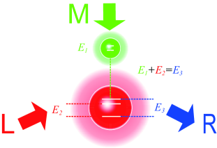
Figure 1: (Colour online) A modulation qubit in contact with the heat bath M and a qutrit connected to a heat bath L and the heat bath R are strongly coupled with each other, which acts as a quantum thermal device. The ground state and the first excited state of the qutrit are greatly separated, while the transition between the first and the second excited states is resonantly coupled to the modulation qubit.

Our model as sketched in Fig. 1, consists of a qubit as the modulation qubit which is in contact with a heat bath M with the temperature $T_{M}$ and simultaneously interacts with a target qutrit which is in contact with a heat bath L and a heat bath R with their temperatures denoted by $T_{L}$ and $T_{R}$. In the following, we will demonstrate that the weak heat current through the modulation qubit can be used to switch on/off, modulate and stabilize the heat currents through the target qutrit from the L bath to the R bath (or in the opposite direction). In particular, as a key feature of the transistor, it can be seen that the amplification of the weak heat current can also be realized by this model.

To show this, let’s turn to the dynamical procedure of our model. For simplicity, we would like to suppose that the ground-state energies are zero for both the qubit and the qutrit. Let ${\left|1\right\rangle}_{1}={\left[1,0\right]}^{T}$ denote the excited state of the qubit with the energy $E_{1}$ and ${\left|1\right\rangle}_{2}={\left[0,1,0\right]}^{T}$ and ${\left|2\right\rangle}_{2}={\left[1,0,0\right]}^{T}$ denote two excited states of the qutrit, respectively, corresponding to the energies $E_{2}$ and $E_{3}$. In addition, we suppose the qubit and the qutrit interact with each other via the Hamiltonian

$$H_{I}=g(\left|11\right\rangle\left\langle 02\right|+\left|02\right\rangle\left\langle 11\right|)$$ (1)

with $g$ representing the coupling strength, so the Hamiltonian of the bipartite interacting system reads

$$H_{S}=H_{0}+H_{I},$$ (2)

where the free Hamiltonian is

$$H_{0}=E_{1}{\left|1\right\rangle}_{1}\left\langle 1\right|+E_{2}{\left|1\right\rangle}_{2}\left\langle 1\right|+E_{3}{\left|2\right\rangle}_{2}\left\langle 2\right|.$$ (3)

Here we consider the resonant coupling, i. e., $E_{1}+E_{2}=E_{3}$ and we set the Boltzmann constant and the Plank constant to be unit, i. e., $\hbar=k_{B}=1$. Now let’s consider the qubit-qutrit system interacts with three heat baths which are described by the quantized radiation field. The free Hamiltonian of the three baths reads

$$H_{\mu}=\sum_{k}\omega_{\mu k}b_{\mu k}^{\dagger}b_{\mu k},\mu=L,M,R,$$ (4)

where $\omega_{\mu k}$ and $b_{\mu k}$ denote the frequency and the annihilation operator of the bath modes with $[b_{\mu k}^{\dagger},b_{\nu k^{{}^{\prime}}}]=\delta_{\mu,\nu}\delta_{k,k^{{}^{\prime}}},[b_{\mu k}^{\dagger},b_{\nu k^{{}^{\prime}}}^{\dagger}]=0,[b_{\mu k},b_{\nu k^{{}^{\prime}}}]=0$. The interaction Hamiltonian between the system and the baths is given by

$$H_{SB}= \sum_{k}f_{Lk}(b_{Lk}^{\dagger}{\left|0\right\rangle}_{2}\left\langle 1\right|+b_{Lk}{\left|1\right\rangle}_{2}\left\langle 0\right|)$$ (5)

$$+ \sum_{k}f_{Mk}(b_{Mk}^{\dagger}{\left|0\right\rangle}_{1}\left\langle 1\right|+b_{Mk}{\left|1\right\rangle}_{1}\left\langle 0\right|)$$

$$+ \sum_{k}f_{Rk}(b_{Rk}^{\dagger}{\left|0\right\rangle}_{2}\left\langle 2\right|+b_{Rk}{\left|2\right\rangle}_{2}\left\langle 0\right|),$$

where $f_{\mu k}$ denotes the coupling constants between the $k$th mode in the $\mu$th bath and the corresponding energy levels of the system. Thus the Hamiltonian of the whole open system can be given as

$$H_{total}=H_{S}+\sum_{\mu}H_{\mu}+H_{SB}.$$ (6)

Based on such a Hamiltonian (6), one can derive the dynamical equation of the open system, i. e., the master equation Breuer and Petruccione (2002). One can note that $H_{S}$ can be diagonalized as $H_{S}=\sum_{i=1,2,...,6}{\lambda}_{i}\left|{\lambda}_{i}\right\rangle\left\langle{\lambda}_{i}\right|$, where the eigenvalues are given by ${\left|\lambda\right\rangle}^{T}=[\lambda_{1},\lambda_{2},...,\lambda_{6}]=[E_{1}+E_{3},E_{3}-g,E_{1},E_{3}+g,E_{2},0]$, and the corresponding eigenstates are

$$\begin{array}[]{ccc}\left|\lambda_{1}\right\rangle=\left|12\right\rangle,\ \left|\lambda_{2}\right\rangle=\frac{1}{\sqrt{2}}(\left|11\right\rangle-\left|02\right\rangle),\ \left|\lambda_{3}\right\rangle=\left|10\right\rangle,\\ \left|\lambda_{4}\right\rangle=\frac{1}{\sqrt{2}}(\left|11\right\rangle+\left|02\right\rangle),\ \left|\lambda_{5}\right\rangle=\left|01\right\rangle,\ \left|\lambda_{6}\right\rangle=\left|00\right\rangle.\end{array}$$ (7)

In the $H_{S}$ presentation, the interaction Hamiltonian $H_{SB}$ can be rewritten as

$$H_{SB}=\sum_{\mu,k,j}f_{\mu k}(b_{\mu k}^{\dagger}V_{\mu l}(\omega_{\mu l})+b_{\mu k}V_{\mu l}^{\dagger}(\omega_{\mu l})),$$

where $V_{\mu l}(\omega_{\mu l})$ stands for the eigenoperator of $H_{S}$ corresponding to the eigenfrequency $\omega_{\mu l}$ with the relation $[H_{S},V_{\mu l}(\omega_{\mu l})]=-\omega_{\mu l}V_{\mu l}(\omega_{\mu l})$. The concrete expressions of the eigenoperators are given in Appendix A. It is clear that the transitions $\left|\lambda_{3}\right\rangle\leftrightarrow\left|\lambda_{2}\right\rangle$, $\left|\lambda_{6}\right\rangle\leftrightarrow\left|\lambda_{5}\right\rangle$, $\left|\lambda_{3}\right\rangle\leftrightarrow\left|\lambda_{4}\right\rangle$ are driven by the bath $L$, $\left|\lambda_{6}\right\rangle\leftrightarrow\left|\lambda_{3}\right\rangle$, $\left|\lambda_{5}\right\rangle\leftrightarrow\left|\lambda_{2}\right\rangle$, $\left|\lambda_{4}\right\rangle\leftrightarrow\left|\lambda_{1}\right\rangle$, $\left|\lambda_{5}\right\rangle\leftrightarrow\left|\lambda_{4}\right\rangle$, $\left|\lambda_{2}\right\rangle\leftrightarrow\left|\lambda_{1}\right\rangle$ are driven by the bath $M$, and $\left|\lambda_{6}\right\rangle\leftrightarrow\left|\lambda_{2}\right\rangle$, $\left|\lambda_{6}\right\rangle\leftrightarrow\left|\lambda_{4}\right\rangle$, $\left|\lambda_{3}\right\rangle\leftrightarrow\left|\lambda_{1}\right\rangle$ are driven by the bath $R$. Following the standard procedure Breuer and Petruccione (2002), within the Born-Markovian approximation and the secular approximation, one can obtain the master equation in Schrödinger picture as

$$\dot{\rho}=-{i}[H_{S},\rho]+\mathcal{L}_{L}[\rho]+\mathcal{L}_{M}[\rho]+\mathcal{L}_{R}[\rho],$$ (8)

where the dissipator $\mathcal{L}_{\mu}[\rho]$ is given by

$$\mathcal{L}_{\mu}[\rho]=\sum_{l}J_{\mu}(-\omega_{\mu l})[2V_{\mu l}(\omega_{\mu l})\rho V_{\mu l}^{\dagger}(\omega_{\mu l})$$

$$-\{V_{\mu l}^{\dagger}(\omega_{\mu l})V_{\mu l}(\omega_{\mu l}),\rho\}]+J_{\mu}(+\omega_{\mu l})[2V_{\mu l}^{\dagger}(\omega_{\mu l})\rho V_{\mu l}(\omega_{\mu l})$$

$$-\{V_{\mu l}(\omega_{\mu l})V_{\mu l}^{\dagger}(\omega_{\mu l}),\rho\}],$$ (9)

with the spectral densities defined by

$$J_{\mu}(+\omega_{\mu l})=\gamma_{\mu}(\omega_{\mu l})n(\omega_{\mu l}),$$ (10)

$$J_{\mu}(-\omega_{\mu l})=\gamma_{\mu}(\omega_{\mu l})[n(\omega_{\mu l})+1],$$ (11)

and the average photon number given by

$$n(\omega_{\mu l})=\frac{1}{e^{\frac{\omega_{\mu l}}{T_{\mu}}}-1}$$ (12)

corresponding to the frequency $\omega_{\mu l}$ and the temperature $T_{\mu}$. Due to the secular approximation, it requires $\gamma_{\mu}(\omega_{\mu l})\ll\{|\omega_{\mu l}-\omega_{\mu l^{{}^{\prime}}}\pm 2g|,g\}$ which implies the strong internal coupling. In addition, we assume $\gamma_{\mu}(\omega_{\mu l})=\gamma_{\mu}$ independent of the transition frequency for simplicity.

III Steady state of the open system and the heat currents

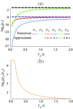
Figure 2: (Colour online) (a) Numerical (solid lines) and approximate (dashed lines) populations versus $T_{M}$ for the steady state. The lines from top to bottom at $T_{M}/E=2$ correspond to $\rho_{66}$, $\rho_{33}$, $\rho_{55}$, $\rho_{22}$, $\rho_{44}$, $\rho_{11}$. (b) The ratio $\rho_{22}/\rho_{44}$ versus $T_{M}$ for the steady state. Here $E_{1}=4E$, $E_{2}=40E$, $E_{3}=E_{1}+E_{2}=44E$, $g=0.75E_{1}$, $\gamma=0.01E_{1}$, $T_{L}=2E$, $T_{R}=0.2E$. For both figures, one can find that $\rho_{22}$ is less than $\rho_{33}$, $\rho_{55}$ and $\rho_{66}$, in the meanwhile, $\rho_{11}$ is less than $\rho_{44}$ which is much less than $\rho_{22}$. In this sense, $\rho_{11}$ and $\rho_{44}$ can be safely neglected to a good approximation.

To demonstrate the functions of a thermal transistor, we need to study the steady-state thermal behavior of the open system. So the first key task is to find the steady solution of the master equation Eq. (8), namely, to solve $\dot{\rho}^{S}=0$ (or Eq. (8) with $t\rightarrow\infty$). To do so, we rewrite the master equation for the steady state as

$$\sum_{\mu=M,L,R}\mathbf{M}_{\mu}\left|\rho\right\rangle=0,$$ (13)

$$\rho_{ij}^{S}=0,i\neq j,$$

where $\left|\rho\right\rangle^{T}=[\rho_{11}^{S},\rho_{22}^{S},\rho_{33}^{S},\rho_{44}^{S},\rho_{55}^{S},\rho_{66}^{S}]$ with

$$\mathbf{M}_{L} =C_{2,1;3,2}\mathbf{J}_{L1}C_{2,1;3,2}^{\dagger}$$

$$+2C_{5,1;6,2}\mathbf{J}_{L2}C_{5,1;6,2}^{\dagger}+C_{3,1;4,2}\mathbf{J}_{L3}C_{3,1;4,2}^{\dagger},$$ (14)

$$\mathbf{M}_{M} =2C_{3,1;6,2}\mathbf{J}_{M1}C_{3,1;6,2}^{\dagger}$$

$$+C_{1,1;4,2}\mathbf{J}_{M2}C_{1,1;4,2}^{\dagger}+C_{2,1;5,2}\mathbf{J}_{M2}C_{2,1;5,2}^{\dagger}$$

$$+C_{1,1;2,2}\mathbf{J}_{M3}C_{1,1;2,2}^{\dagger}+C_{4,1;5,2}\mathbf{J}_{M3}C_{4,1;5,2}^{\dagger},$$ (15)

$$\mathbf{M}_{R} =C_{2,1;6,2}\mathbf{J}_{R1}C_{2,1;6,2}^{\dagger}$$

$$+C_{4,1;6,2}\mathbf{J}_{R2}C_{4,1;6,2}^{\dagger}+C_{1,1;3,2}\mathbf{J}_{R3}C_{1,1;3,2}^{\dagger}.$$ (16)

Here $\mathbf{J}_{\mu l}=\left|2\right\rangle\left\langle 2\right|\otimes\begin{pmatrix}-A_{\mu l}&B_{\mu l}\\ A_{\mu l}&-B_{\mu l}\end{pmatrix}$ with $A_{\mu l}=\gamma_{\mu}(n(\omega_{\mu l})+1)$ and $B_{\mu l}=\gamma_{\mu}n(\omega_{\mu l})$, and $C_{i,j;m,n}=\left|i\right\rangle\left\langle j\right|+\left|m\right\rangle\left\langle n\right|$ with $\left\{\left|i\right\rangle\right\}$ representing the orthonormal basis of $6$-dimensional Hilbert space. One can find that Eq. (13) is analytically solvable, but the concrete expression is so tedious that it is impossible to present explicitly here. So we make some reasonable approximations in order to give an explicit presentation. Here all the involved parameters are taken as $E_{1}=4E$, $E_{2}=40E$, $E_{3}=E_{1}+E_{2}=44E$, $g=0.75E_{1}$, $\gamma=0.01E_{1}$, $T_{L}=2E$, $T_{R}=0.2E$ and $T_{M}<$ $T_{L}$. Under this condition, the two higher energy levels $\left|\lambda_{1}\right\rangle$ and $\left|\lambda_{4}\right\rangle$ of $H_{S}$ are difficult to excite, so one can easily check that the populations of $\rho_{11}^{S}$ and $\rho_{44}^{S}$ are much less than others, which can be seen from Fig. 2 (a) and (b). This means that the contributions of these two energy levels $\left|\lambda_{1}\right\rangle$ and $\left|\lambda_{4}\right\rangle$ can be safely neglected to some good approximation. Thus we can replace the irrelevant matrix entries in Eq. (13) by zero. In this way, the simplified Eq. (13) can be written as

$$\sum_{\mu=M,L,R}\mathbf{\tilde{M}}_{\mu}\left|\tilde{\rho}\right\rangle=0,$$ (17)

$$\rho_{22}^{S}+\rho_{33}^{S}+\rho_{55}^{S}+\rho_{66}^{S}=1,$$

where $\mathbf{\tilde{M}}_{L}=C_{2,1;3,2}\mathbf{J}_{L1}C_{2,1;3,2}^{\dagger}+2C_{5,1;6,2}\mathbf{J}_{L2}C_{5,1;6,2}^{\dagger}$, $\mathbf{\tilde{M}}_{M}=2C_{3,1;6,2}\mathbf{J}_{M1}C_{3,1;6,2}^{\dagger}+C_{1,1;4,2}\mathbf{J}_{M2}C_{1,1;4,2}^{\dagger}+C_{2,1;5,2}\mathbf{J}_{M2}C_{2,1;5,2}^{\dagger}$, $\mathbf{\tilde{M}}_{R}=C_{2,1;6,2}\mathbf{J}_{R1}C_{2,1;6,2}^{\dagger}$ and $\left|\tilde{\rho}\right\rangle=[0,\rho_{22}^{S},\rho_{33}^{S},0,\rho_{55}^{S},\rho_{66}^{S}]^{T}$. As a result, one can obtain

$$\rho_{22}^{S}=\frac{D_{2}}{D},\rho_{33}^{S}=\frac{D_{3}}{D},\rho_{55}^{S}=\frac{D_{5}}{D},\rho_{66}^{S}=\frac{D_{6}}{D},$$ (18)

where

$$D_{2} =2A_{L2}\left[2B_{M1}B_{L1}+B_{R1}\left(2A_{M1}+B_{L1}\right)\right]+B_{M2}$$

$$\times\left[2B_{M1}B_{L1}+\left(2A_{M1}+B_{L1}\right)\left(2B_{L2}+B_{R1}\right)\right],$$ (19)

$$D_{3} =2B_{M1}\left[2A_{M2}A_{L2}+A_{R1}(2A_{L2}+B_{M2})\right]+A_{L1}$$

$$\times\left[2A_{L2}(2B_{M1}+B_{R1})+B_{M2}(2B_{M1}+2B_{L2}+B_{R1})\right],$$ (20)

$$D_{5} =2B_{L2}\left[A_{R1}B_{L1}+2A_{M1}(A_{L1}+A_{R1})\right]+A_{M2}$$

$$\times\left[2B_{M1}B_{L1}+(2A_{M1}+B_{L1})(2B_{L2}+B_{R1})\right],$$ (21)

$$D_{6} =B_{L1}\left[2A_{M2}A_{L2}+A_{R1}(2A_{L2}+B_{M2})\right]+2A_{M1}$$

$$\times\left[2A_{M2}A_{L2}+(A_{L1}+A_{R1})(2A_{L2}+B_{M2})\right],$$ (22)

$$D =D_{2}+D_{3}+D_{5}+D_{6}.$$

With the solutions of Eq. (18), one can calculate the heat currents subject to different baths as Szczygielski et al. (2013); Alicki et al. (2006); Levy et al. (2012); Kolář et al. (2012)

$$\dot{Q}_{\mu}={Tr}(H_{S}\mathcal{L}_{\mu}[\rho^{S}])\approx\left\langle\lambda\right|\mathbf{\tilde{M}}_{\mu}\left|\tilde{\rho}\right\rangle,$$ (23)

which can be explicitly given by

$$\dot{Q}_{L} =-\omega_{L1}\Gamma_{23}^{L}-2\omega_{L2}\Gamma_{56}^{L},$$ (24)

$$\dot{Q}_{M} =-2\omega_{M1}\Gamma_{36}^{M}-\omega_{M2}\Gamma_{25}^{M},$$ (25)

$$\dot{Q}_{R} =-\omega_{R1}\Gamma_{26}^{R},$$ (26)

where

$$\Gamma_{i,j}^{\mu}=\gamma_{\mu}[(n_{\mu}(\lambda_{i}-\lambda_{j})+1)\rho_{ii}^{S}-n_{\mu}(\lambda_{i}-\lambda_{j})\rho_{jj}^{S}]$$ (27)

denotes the net decay rate from the state $\left|i\right\rangle$ to $\left|j\right\rangle$ due to the coupling with the $\mu$th bath. One knows that $\dot{Q}_{\mu}>0$ means the heat flows out of the $\mu$th bath and $\dot{Q}_{\mu}<0$ corresponds to the heat flows into the $\mu$th bath. It can be easily checked that $\dot{Q}_{L}+\dot{Q}_{M}+\dot{Q}_{R}=0$ corresponding to the energy conservation law. In the next section, we will show that the heat currents can be effectively controlled and hence our thermal device can realize the functions of a thermal transistor.

IV The functions as a transistor

Now we will show that the weak modulation heat current $\dot{Q}_{M}$ can modulate, switch, and stabilize the output currents through the target qutrit, moreover, our model can realize the typical function as a thermal transistor—the amplification of the weak modulation heat current $\dot{Q}_{M}$, that is, the left current $\dot{Q}_{L}$ or the right one $\dot{Q}_{R}$ can become greatly larger than $\dot{Q}_{M}$ with a dynamical amplification factor $\alpha$ defined as

$$\alpha_{L,R}=\frac{\partial\dot{Q}_{L,R}}{\partial\dot{Q}_{M}}.$$ (28)

If the amplification factor $\alpha_{L,R}>1$, we can say the transistor effect is achieved. In particular, the larger $\alpha_{L,R}$ is, the better transistor effect is obtained.

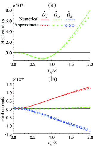
Figure 3: (Colour online) Three thermal currents $\dot{Q}_{L}$, $\dot{Q}_{M}$, and $\dot{Q}_{R}$ via numerical and approximate methods at steady state versus $T_{M}$. The parameters are same as in Fig. 2.

Switch. –In order to show the function as a quantum thermal switch, we plot the three heat currents in Fig. 3. It is obvious that all the three heat currents are very small even close to zero in the low temperature $T_{M}$ regime, i.e., $T_{M}/E\lesssim 0.3$. Especially $\dot{Q}_{L,R}$ in the low temperature $T_{M}$ regime are much smaller than those in the large $T_{M}$ regime. Therefore, if the heat currents are neglectfully small, we can think that the heat conduction is prevented between the bath L and the bath R. In this sense, one can find that our model can be considered to be at the “off” state for $T_{M}/E\lesssim 0.3$. With the increase of $T_{M}$, the heat currents $\dot{Q}_{L,R}$ are gradually increased, namely, the switch is gradually open and the heat is allowed to transport between the bath L and the bath R. It is especially noted that if the switch is off, $T_{M}$ can be taken in a large safe range so long as $T_{M}/E\lesssim 0.3$ is satisfied. Actually, one can always define an exact critical small value of the allowable heat current based on the practical case. When the heat current value is less than this critical value, one can think the switch is off and when the heat current is larger than the critical value, the switch is on.

Modulation. –The modulation function means the heat current can be controlled continuously from a small value to a large one by another much smaller continuous current. From Fig. 3, one can find that in the whole range of $T_{M}$, $\dot{Q}_{M}$ always keeps greatly smaller than $\dot{Q}_{L,R}$, while $\dot{Q}_{L,R}$ ranges from a small value (can reach zero) at low $T_{M}$ to a large one for a large $T_{M}$. In this perspective, the two currents $\dot{Q}_{L,R}$ are modulated by a tiny modulation current $\dot{Q}_{M}$ and the modulation function is realized.

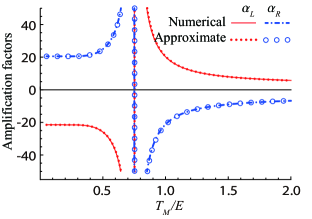
Figure 4: (Colour online) Two amplification factors $\alpha_{L}$ and $\alpha_{R}$ via numerical and approximate methods at steady state versus $T_{M}$. The parameters are same as in Fig. 2.

Amplification. –The crucial feature of a transistor is the function of amplification, namely, the weak modulation heat current $\dot{Q}_{M}$ amplifies (or induces) a strong heat current which transports between the bath L and the bath R. In fact, it is apparent that from Fig. 3, the current $\dot{Q}_{M}$ varies gently when $0.3\lesssim T_{M}/E$, but the currents $\dot{Q}_{L,R}$ are changed rapidly, which implies the amplification is achieved. However, in order to precisely describe the amplification effect, one has to employ the amplification factor $\alpha$ defined in Eq. (28). In Fig. 4, we present the two amplification factors $\alpha_{L}$ and $\alpha_{R}$ versus $T_{M}$. The two amplification factors are obviously larger than $1$, which shows that the amplification effect indeed exits in our model. At the low temperature range $0<T_{M}/E<0.5$, the heat current is stably amplified due to almost the same amplification factors (about $20$). At the range $0.5<T_{M}/E<1$, the amplification factors strongly depend on the temperature $T_{M}$. This can be regarded as a sensitive region which means a tiny change of the modulation current $\dot{Q}_{M}$ can lead to the drastic change of the currents $\dot{Q}_{L,R}$. The region $T_{M}/E>1$ can be considered as the weak stable amplification region. But the factors $\alpha_{L,R}$ are still larger than 1, for example, $\alpha_{L}=5.749$ and $\alpha_{R}=-6.749$ for $T_{M}/E=2.0$. Thus, one can select the proper working region based on what kind of amplification is required in the practical scenario.

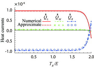
Figure 5: (Colour online) Three thermal currents $\dot{Q}_{L}$, $\dot{Q}_{M}$, and $\dot{Q}_{R}$ via numerical and approximate methods at steady state versus $T_{R}$. Here $T_{M}/E=1.5$ and the parameters are same as in Fig. 2.

Stabilizer. –In fact, our model can also work for a stabilizer of heat currents, namely, the heat currents $\dot{Q}_{L,R}$ are not sensitive to the change of the temperature of $T_{R}$ (the low-temperature terminal). To illustrate such a function, we plot the three heat currents versus versus $T_{R}$ in Fig. 5. One can see that when the temperature $T_{R}$ varies from $0$ to about $T_{R}$ along the horizontal axis, the heat currents $\dot{Q}_{L,R}$ are kept almost in the horizontal lines, that is, there is no obvious change of the heat currents $\dot{Q}_{L,R}$. In fact, a direct understanding of this phenomenon can be obtained by our Eq. (26) and Eq. (27) where the fluctuation of the lower temperature at the $R$ terminal subject to the large transition frequency between the energy levels $\left|\lambda_{2}\right\rangle$ and $\left|\lambda_{6}\right\rangle$ can not lead to the considerable fluctuation of the net decay rate. In other words, the large fluctuations of $T_{R}$ cannot drastically influence the heat currents $\dot{Q}_{L,R}$, namely, $\dot{Q}_{L,R}$ in the given temperature range are stabilized.

Finally, we emphasize that the thermal transistor proposed in this paper is a thermal device with three terminals. Here we use the heat $Q_{M}$ as the “modulation” terminal which controls the heat currents between the other two terminals. What we would like to emphasize is that the choice of the “modulation” terminal is not unique. In the Appendix B, we have numerically studied the cases with $Q_{L}$ and $Q_{R}$ as the “modulation” terminal respectively. It is shown that in both cases our proposed thermal device can realize all the mentioned functions as a transistor including the functions of the switch, the modulation and the amplification. As to the function of the stabilizer, one can also find that if the heat current $Q_{L}$ as the low-temperature terminal, the heat currents $Q_{L,R}$ can also be stabilized. In fact, throughout of the paper, we intend to fix $T_{M}$ is a medium temperature between $T_{L}$ and $T_{R}$, which is enough for us to show our device as a transistor. If other parameters are selected, one can find that the function as a transistor can be realized in different cases which are not indicated extensively. We also consider the case of the weak internal coupling. One can find that the transistor effect still exists, but the price is that the heat currents will be reduced to the very low level (two small). This actually coincides with Refs. Yu and Zhu (2014); Man and Xia (2017) working in the cooling regime, where the strong internal coupling suppresses the cooling, but the current model works in the heating regime. An intuitive understanding could be that the suppression of cooling implies the enhancement of heating. In addition, one can also find that compared with Ref. Joulain et al. (2016), we have realized the similar functions with less energy levels and particles with a different mechanism.

V Discussion and conclusion

Before the end, we would like to give some discussions about the potential design in the superconducting systems. As we know, the superconducting artificial atom provides a possibility to realize a $\Delta$-type system allowing different transitions between the three levels You and Nori (2011); Buluta et al. (2011). One distinct advantage is that the energy gap can be customized freely, for instance, via changing magnetic flux in a circuit QED architecture and another advantage is that the coupling between the superconducting artificial atoms can be easily tuned to be strong Niskanen et al. (2007); Hime et al. (2006). The energy gap of superconducting circuits ranges from $1$GHz to $10$ GHz or even higher and the strong coupling is about the order of $1$ GHz via mutual inductance or capacitance. The choice of the coupling energy levels are well guaranteed by the rotating wave approximation so long as the large detuning is adjusted. The coupling between the system and a bath can be achieved via resonator and a resistor acts as a bath Karimi et al. (2017); Cottet et al. (2017). In fact, the reservoir could be directly tailored with the desired bath spectra by reservoir engineering, which was described in detail and applied in many cases Scovil and Schulz-DuBois (1959); Gelbwaser-Klimovsky et al. (2013); Myatt et al. (2000); Gröblacher et al. (2015). In addition, one can note that autonomous quantum refrigerator in a circuit QED architecture based on a Josephson junction and a quantum heat switch based on coupled superconducting qubits have been proposed in Ref. Hofer et al. (2016); Karimi et al. (2017), and other relevant investigations about heat transport can also be found in their references.

In conclusion, we have presented a thermal device to realize the functions of a thermal transistor by utilizing the strong internal coupling between the qubit and the qutrit which are connected to three baths with different temperatures. We mainly emphasize the functions as the thermal switch, the modulation, the stabilization, and the amplification which are rigorously demonstrated by both the numerical and the approximately analytic procedures. It is shown that the adjustable energy levels in the qutrit system plays the significant role in the design of the thermal transistor. We also present the possible experimental scheme to realize the scheme.

Appendix A Eigenoperators of the system

In order to derive the master equation, we would like to emphasize that the Born-Markov approximation and secular approximation will be used following the standard procedure Breuer and Petruccione (2002). We also require a large internal coupling $g$ to satisfy the secular approximation condition. Considering the total Hamiltonian including the three baths as

$$H=H_{S}+H_{SB}+\sum_{\mu}H_{\mu},$$ (29)

we can first diagonalize the Hamiltonian $H_{S}$ and then in the $H_{S}$ representation derive the eigenoperators with their corresponding eigenfrequencies $\omega_{\mu l}$ as

$$V_{L1}=\frac{1}{\sqrt{2}}(\left|\lambda_{3}\right\rangle\left\langle\lambda_{2}\right|),\quad\omega_{L1}=E_{2}-g,$$ (30)

$$V_{L2}=\left|\lambda_{6}\right\rangle\left\langle\lambda_{5}\right|,\quad\omega_{L2}=E_{2},$$ (31)

$$V_{L3}=\frac{1}{\sqrt{2}}(\left|\lambda_{3}\right\rangle\left\langle\lambda_{4}\right|),\quad\omega_{L3}=E_{2}+g,$$ (32)

$$V_{M1}=\left|\lambda_{6}\right\rangle\left\langle\lambda_{3}\right|,\quad\omega_{M1}=E_{1},$$ (33)

$$V_{M2}=\frac{1}{\sqrt{2}}(\left|\lambda_{5}\right\rangle\left\langle\lambda_{2}\right|+\left|\lambda_{4}\right\rangle\left\langle\lambda_{1}\right|),\quad\omega_{M2}=E_{1}-g,$$ (34)

$$V_{M3}=\frac{1}{\sqrt{2}}(\left|\lambda_{5}\right\rangle\left\langle\lambda_{4}\right|-\left|\lambda_{2}\right\rangle\left\langle\lambda_{1}\right|),\quad\omega_{M3}=E_{1}+g,$$ (35)

$$V_{R1}=\frac{1}{\sqrt{2}}(\left|\lambda_{6}\right\rangle\left\langle\lambda_{2}\right|),\quad\omega_{R1}=E_{3}-g,$$ (36)

$$V_{R2}=-\frac{1}{\sqrt{2}}(\left|\lambda_{6}\right\rangle\left\langle\lambda_{4}\right|),\quad\omega_{R2}=E_{3}+g,$$ (37)

$$V_{R3}=\left|\lambda_{3}\right\rangle\left\langle\lambda_{1}\right|,\quad\omega_{R3}=E_{3}.$$ (38)

The master equation can be directly obtained by substituting these eigenoperators into the standard Lindbladian master equation

$$\frac{d\rho_{S}}{dt} =-i[H_{S},\rho_{S}]$$

$$+\sum^{N^{2}-1}_{k=1}\gamma_{k}(A_{k}\rho_{S}A^{\dagger}_{k}-\frac{1}{2}A^{\dagger}_{k}A_{k}\rho_{S}-\frac{1}{2}\rho_{S}A^{\dagger}_{k}A_{k}).$$ (39)

What we should pay attention to is the $\gamma$’s formula. The master equation for our model can be found in the main text, we will not show it here again.

Appendix B The transistor with different modulation terminals

In the main text, we consider $\dot{Q}_{M}$ as the modulation current which can effectively control the heat current between the other two terminals. Here we will show that $\dot{Q}_{L/R}$ can also be used as the modulation current, which is explicitly illustrated in Fig. 6 and Fig. 7. It is obvious that the functions of interests like the switch, the modulation and the amplification can be realized in the different parameter ranges. In addition, in Fig. 8 we plot the function of the heat current stabilization subject to the temperature fluctuation at the terminal L. Although a different lower-temperature terminal is used contrast to the main text, the heat currents are only robust to the temperature fluctuation of the lower-temperature terminal.

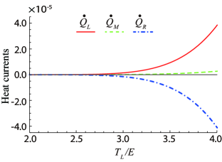
Figure 6: (Colour online) Three thermal currents $\dot{Q}_{L}$, $\dot{Q}_{M}$, and $\dot{Q}_{R}$ via numerical method at steady state versus $T_{L}$. Here $T_{M}/E=4$, $T_{R}/E=2$ and the other parameters are same as in Fig. 2.

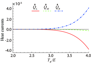
Figure 7: (Colour online) Three thermal currents $\dot{Q}_{L}$, $\dot{Q}_{M}$, and $\dot{Q}_{R}$ via numerical method at steady state versus $T_{R}$. Here $T_{M}/E=4$, $T_{L}/E=2$ and the other parameters are same as in Fig. 2.

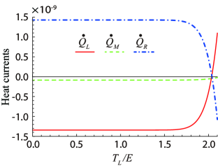
Figure 8: (Colour online) Three thermal currents $\dot{Q}_{L}$, $\dot{Q}_{M}$, and $\dot{Q}_{R}$ via numerical method at steady state versus $T_{L}$. Here $T_{M}/E=1.5$, $T_{R}/E=2$ and the other parameters are same as in Fig. 2.

References

- Lashkaryov (1941) V. E. Lashkaryov, “Investigations of a barrier layer by the thermoprobe method,” Izv. Akad. Nauk SSSR, Ser. Fiz. 5, 422 (1941).
- Bardeen and Brattain (1998) J. Bardeen and W. H. Brattain, “The transistor, a semiconductor triode,” Proc. IEEE 86, 29 (1998).
- Chang et al. (2006) C. W. Chang, D. Okawa, A. Majumdar, and A. Zettl, “Solid-state thermal rectifier.” Science 314, 1121 (2006).
- Scheibner et al. (2008) R. Scheibner, M. König, D. Reuter, A. D. Wieck, C. Gould, H. Buhmann, and L. W. Molenkamp, “Quantum dot as thermal rectifier,” New J. Phys. 10, 083016 (2008).
- Kobayashi et al. (2009) W. Kobayashi, Y. Teraoka, and I. Terasaki, “An oxide thermal rectifier,” Appl. Phys. Lett. 95, 171905 (2009).
- van Zwol et al. (2012a) P. J. van Zwol, L. Ranno, and J. Chevrier, “Tuning near field radiative heat flux through surface excitations with a metal insulator transition.” Phys. Rev. Lett. 108, 234301 (2012a).
- van Zwol et al. (2012b) P. J. van Zwol, L. Ranno, and J. Chevrier, “Emissivity measurements with an atomic force microscope,” J. Appl. Phys. 111, 063110 (2012b).
- Ito et al. (2016) K. Ito, K. Nishikawa, and H. Iizuka, “Multilevel radiative thermal memory realized by the hysteretic metal-insulator transition of vanadium dioxide,” Appl. Phys. Lett. 108, 053507 (2016).
- Ben-Abdallah and Biehs (2013) P. Ben-Abdallah and S. A. Biehs, “Phase-change radiative thermal diode,” Appl. Phys. Lett. 103, 191907 (2013).
- Yang et al. (2013) Y. Yang, S. Basu, and L. P. Wang, “Radiation-based near-field thermal rectification with phase transition materials,” Appl. Phys. Lett. 103, 163101 (2013).
- Ito et al. (2014) K. Ito, K. Nishikawa, H. Iizuka, and H. Toshiyoshi, “Experimental investigation of radiative thermal rectifier using vanadium dioxide,” Appl. Phys. Lett. 105, 253503 (2014).
- Ben-Abdallah and Biehs (2014) P. Ben-Abdallah and S. A. Biehs, “Near-field thermal transistor.” Phys. Rev. Lett. 112, 044301 (2014).
- Joulain et al. (2015) K. Joulain, Y. Ezzahri, J. Drevillon, and P. Ben-Abdallah, “Modulation and amplification of radiative far field heat transfer: Towards a simple radiative thermal transistor,” Appl. Phys. Lett. 106, 133505 (2015).
- Wang et al. (2013) L. Wang, B. Hu, and B. W. Li, “Validity of fourier’s law in one-dimensional momentum-conserving lattices with asymmetric interparticle interactions,” Phys. Rev. E 88, 052112 (2013).
- Landi and de Oliveira (2013) G. T. Landi and M. J. de Oliveira, “Fourier’s law from a chain of coupled anharmonic oscillators under energy-conserving noise,” Phys. Rev. E 87, 052126 (2013).
- Chang et al. (2008) C. W. Chang, D. Okawa, H. Garcia, A. Majumdar, and A. Zettl, “Breakdown of fourier’s law in nanotube thermal conductors,” Phys. Rev. Lett. 101, 075903 (2008).
- Manzano et al. (2012) D. Manzano, M. Tiersch, A. Asadian, and H. J. Briegel, “Quantum transport efficiency and fourier’s law,” Phys. Rev. E 86, 061118 (2012).
- Zhang and Zhao (2002) Y. Zhang and H. Zhao, “Heat conduction in a one-dimensional aperiodic system,” Phys. Rev. E 66, 026106 (2002).
- Mao et al. (2005) J. W. Mao, Y. Q. Li, and Y. Y. Ji, “Role of chaos in one-dimensional heat conductivity,” Phys. Rev. E 71, 061202 (2005).
- Hu et al. (2006) B. Hu, D. He, L. Yang, and Y. Zhang, “Asymmetric heat conduction through a weak link,” Phys. Rev. E 74, 060101 (2006).
- Levy and Kosloff (2014) A. Levy and R. Kosloff, “The local approach to quantum transport may violate the second law of thermodynamics,” Europhys. Lett. 107, 20004 (2014).
- Landsberg (1956) P. T. Landsberg, “Foundations of thermodynamics,” Rev. Mod. Phys. 28, 363 (1956).
- Levy et al. (2012) A. Levy, R. Alicki, and R. Kosloff, “Quantum refrigerators and the third law of thermodynamics,” Phys. Rev. E 85, 061126 (2012).
- Maruyama et al. (2009) K. Maruyama, F. Nori, and V. Vedral, “Colloquium: The physics of maxwell’s demon and information,” Rev. Mod. Phys. 81, 1 (2009).
- Feldmann and Kosloff (2000) T. Feldmann and R. Kosloff, “Performance of discrete heat engines and heat pumps in finite time,” Phys. Rev. E 61, 4774 (2000).
- Palao et al. (2001) J. P. Palao, R. Kosloff, and J. M. Gordon, “Quantum thermodynamic cooling cycle,” Phys. Rev. E 64, 056130 (2001).
- Arnaud et al. (2002) J. Arnaud, L. Chusseau, and F. Philippe, “Carnot cycle for an oscillator,” Eur. J. Phys. 23, 489 (2002).
- Segal and Nitzan (2006) D. Segal and A. Nitzan, “Molecular heat pump,” Phys. Rev. E 73, 026109 (2006).
- de Tomás et al. (2012) C. de Tomás, A. C. Hernández, and J. M. M. Roco, “Optimal low symmetric dissipation carnot engines and refrigerators,” Phys. Rev. E 85, 010104 (2012).
- Geva and Kosloff (1992) E. Geva and R. Kosloff, “A quantum-mechanical heat engine operating in finite time. a model consisting of spin- systems as the working fluid,” J. Chem. Phys. 96, 3054 (1992).
- Geva and Kosloff (1996) E. Geva and R. Kosloff, “The quantum heat engine and heat pump: An irreversible thermodynamic analysis of the three‐level amplifier,” J. Chem. Phys. 104, 7681 (1996).
- Kosloff and Feldmann (2010) R. Kosloff and T. Feldmann, “Optimal performance of reciprocating demagnetization quantum refrigerators,” Phys. Rev. E 82, 011134 (2010).
- Thomas and Johal (2011) G. Thomas and R. S. Johal, “Coupled quantum otto cycle,” Phys. Rev. E 83, 031135 (2011).
- Feldmann et al. (1996) T. Feldmann, E. Geva, R. Kosloff, and P. Salamon, “Heat engines in finite time governed by master equations,” Am. J. Phys. 64, 485 (1996).
- Feldmann and Kosloff (2003) T. Feldmann and R. Kosloff, “Quantum four-stroke heat engine: Thermodynamic observables in a model with intrinsic friction,” Phys. Rev. E 68, 016101 (2003).
- Quan et al. (2007) H. T. Quan, Y. X. Liu, C. P. Sun, and F. Nori, “Quantum thermodynamic cycles and quantum heat engines,” Phys. Rev. E 76, 031105 (2007).
- Linden et al. (2010) N. Linden, S. Popescu, and P. Skrzypczyk, “How small can thermal machines be? the smallest possible refrigerator,” Phys. Rev. Lett. 105, 130401 (2010).
- Yu and Zhu (2014) C. S. Yu and Q. Y. Zhu, “Re-examining the self-contained quantum refrigerator in the strong-coupling regime,” Phys. Rev. E 90, 052142 (2014).
- Man and Xia (2017) Z. X. Man and Y. J. Xia, “Smallest quantum thermal machine: The effect of strong coupling and distributed thermal tasks,” Phys. Rev. E 96, 012122 (2017).
- Silva et al. (2015) R. Silva, P. Skrzypczyk, and N. Brunner, “Small quantum absorption refrigerator with reversed couplings,” Phys. Rev. E 92, 012136 (2015).
- Abah et al. (2012) O. Abah, J. Roßnagel, G. Jacob, S. Deffner, F. Schmidt-Kaler, K. Singer, and E. Lutz, “Single-ion heat engine at maximum power,” Phys. Rev. Lett. 109, 203006 (2012).
- Roßnagel et al. (2016) J. Roßnagel, S. T. Dawkins, K. N. Tolazzi, O. Abah, E. Lutz, F. Schmidt-Kaler, and K. Singer, “A single-atom heat engine,” Science 352, 325 (2016).
- Scovil and Schulz-DuBois (1959) H. E. D. Scovil and E. O. Schulz-DuBois, “Three-level masers as heat engines,” Phys. Rev. Lett. 2, 262 (1959).
- Alicki (1979) R. Alicki, “The quantum open system as a model of the heat engine,” J. Phys. A 12, L103 (1979).
- Skrzypczyk et al. (2011) P. Skrzypczyk, N. Brunner, N. Linden, and S. Popescu, “The smallest refrigerators can reach maximal efficiency,” J. Phys. A 44, 492002 (2011).
- Wang and Li (2007) L. Wang and B. W. Li, “Thermal logic gates: Computation with phonons,” Phys. Rev. Lett. 99, 177208 (2007).
- Wang and Li (2008) L. Wang and B. W. Li, “Thermal memory: A storage of phononic information,” Phys. Rev. Lett. 101, 267203 (2008).
- Faucheux et al. (1995) L. P. Faucheux, L. S. Bourdieu, P. D. Kaplan, and A. J. Libchaber, “Optical thermal ratchet,” Phys. Rev. Lett. 74, 1504 (1995).
- Zhan et al. (2009) F. Zhan, N. B. Li, S. Kohler, and P. Hänggi, “Molecular wires acting as quantum heat ratchets,” Phys. Rev. E 80, 061115 (2009).
- Hofer et al. (2017) P. P. Hofer, J. B. Brask, M. Perarnau-Llobet, and N. Brunner, “Quantum thermal machine as a thermometer,” Phys. Rev. Lett. 119, 090603 (2017).
- Werlang et al. (2014) T. Werlang, M. A. Marchiori, M. F. Cornelio, and D. Valente, “Optimal rectification in the ultrastrong coupling regime,” Phys. Rev. E 89, 062109 (2014).
- Chen and Wang (2015) T. Chen and X. B. Wang, “Thermal rectification in the nonequilibrium quantum-dots-system,” Physica E 72, 58 (2015).
- Li et al. (2004) B. W. Li, L. Wang, and G. Casati, “Thermal diode: Rectification of heat flux,” Phys. Rev. Lett. 93, 184301 (2004).
- Pereira (2011) E. Pereira, “Sufficient conditions for thermal rectification in general graded materials,” Phys. Rev. E 83, 031106 (2011).
- Wang et al. (2012) J. Wang, E. Pereira, and G. Casati, “Thermal rectification in graded materials,” Phys. Rev. E 86, 010101 (2012).
- Fratini and Ghobadi (2016) F. Fratini and R. Ghobadi, “Full quantum treatment of a light diode,” Phys. Rev. A 93, 023818 (2016).
- Landi et al. (2014) G. T. Landi, E. Novais, M. J. de Oliveira, and D. Karevski, “Flux rectification in the quantum chain,” Phys. Rev. E 90, 042142 (2014).
- Man et al. (2016) Z. X. Man, N. B. An, and Y. J. Xia, “Controlling heat flows among three reservoirs asymmetrically coupled to two two-level systems,” Phys. Rev. E 94, 042135 (2016).
- Jiang et al. (2015) J. H. Jiang, M. Kulkarni, D. Segal, and Y. Imry, “Phonon thermoelectric transistors and rectifiers,” Phys. Rev. B 92, 045309 (2015).
- Joulain et al. (2016) K. Joulain, J. Drevillon, Y. Ezzahri, and J. Ordonez-Miranda, “Quantum thermal transistor,” Phys. Rev. Lett. 116, 200601 (2016).
- Lo et al. (2008) W. C. Lo, L. Wang, and B. W. Li, “Thermal transistor: Heat flux switching and modulating,” J. Phys. Soc. Jpn. 77, 054402 (2008).
- Li et al. (2006) B. W. Li, L. Wang, and G. Casati, “Negative differential thermal resistance and thermal transistor,” Appl. Phys. Lett. 88, 143501 (2006).
- Komatsu and Ito (2011) T. S. Komatsu and N. Ito, “Thermal transistor utilizing gas-liquid transition,” Phys. Rev. E 83, 012104 (2011).
- Joulain et al. (2017) K. Joulain, Y. Ezzahri, and J. Ordonez-Miranda, “Quantum thermal rectification to design thermal diodes and transistors,” Z. Naturforsch. A 72, 163 (2017).
- You and Nori (2011) JQ You and F. Nori, “Atomic physics and quantum optics using superconducting circuits,” Nature 474, 589 (2011).
- Buluta et al. (2011) I. Buluta, S. Ashhab, and F. Nori, “Natural and artificial atoms for quantum computation,” Reports on Progress in Physics 74, 104401 (2011).
- Hofer et al. (2016) P. P. Hofer, M. Perarnau-Llobet, J. B. Brask, R. Silva, M. Huber, and N. Brunner, “Autonomous quantum refrigerator in a circuit qed architecture based on a josephson junction,” Phys. Rev. B 94, 235420 (2016).
- Karimi et al. (2017) B. Karimi, J. P. Pekola, M. Campisi, and R. Fazio, “Coupled qubits as a quantum heat switch,” Quantum Science and Technology 2, 044007 (2017).
- Breuer and Petruccione (2002) H. P. Breuer and F. Petruccione, The Theory of Open Quantum Systems (Oxford University Press, Oxford, UK, 2002).
- Szczygielski et al. (2013) K. Szczygielski, D. Gelbwaser-Klimovsky, and R. Alicki, “Markovian master equation and thermodynamics of a two-level system in a strong laser field,” Phys. Rev. E 87, 012120 (2013).
- Alicki et al. (2006) R. Alicki, D. A. Lidar, and P. Zanardi, “Internal consistency of fault-tolerant quantum error correction in light of rigorous derivations of the quantum markovian limit,” Phys. Rev. A 73, 052311 (2006).
- Kolář et al. (2012) M. Kolář, D. Gelbwaser-Klimovsky, R. Alicki, and G. Kurizki, “Quantum bath refrigeration towards absolute zero: Challenging the unattainability principle,” Phys. Rev. Lett. 109, 090601 (2012).
- Niskanen et al. (2007) A. O. Niskanen, K. Harrabi, F. Yoshihara, Y. Nakamura, S. Lloyd, and JS Tsai, “Quantum coherent tunable coupling of superconducting qubits,” Science 316, 723–726 (2007).
- Hime et al. (2006) T. Hime, P. A. Reichardt, B. L. T. Plourde, T. L. Robertson, C.-E. Wu, A. V. Ustinov, and J. Clarke, “Solid-state qubits with current-controlled coupling,” science 314, 1427–1429 (2006).
- Cottet et al. (2017) N. Cottet, S. Jezouin, L. Bretheau, P. Campagne-Ibarcq, Q. Ficheux, J. Anders, A. Auffèves, R. Azouit, P. Rouchon, and B. Huard, “Observing a quantum maxwell demon at work,” Proceedings of the National Academy of Sciences 114, 7561–7564 (2017).
- Gelbwaser-Klimovsky et al. (2013) D. Gelbwaser-Klimovsky, R. Alicki, and G. Kurizki, “Minimal universal quantum heat machine,” Phys. Rev. E 87, 012140 (2013).
- Myatt et al. (2000) C.J. Myatt, B. E. King, Q. A. Turchette, C. A. Sackett, D. Kielpinski, W. M. Itano, C. Monroe, and D. J. Wineland, “Decoherence of quantum superpositions through coupling to engineered reservoirs,” Nature 403, 269 (2000).
- Gröblacher et al. (2015) S. Gröblacher, A. Trubarov, N. Prigge, G.D. Cole, M. Aspelmeyer, and J. Eisert, “Observation of non-markovian micromechanical brownian motion,” Nature communications 6, 7606 (2015).