NeuTra-lizing Bad Geometry in Hamiltonian Monte Carlo Using Neural Transport
Abstract
Hamiltonian Monte Carlo is a powerful algorithm for sampling from difficult-to-normalize posterior distributions. However, when the geometry of the posterior is unfavorable, it may take many expensive evaluations of the target distribution and its gradient to converge and mix. We propose neural transport (NeuTra) HMC, a technique for learning to correct this sort of unfavorable geometry using inverse autoregressive flows (IAF), a powerful neural variational inference technique. The IAF is trained to minimize the KL divergence from an isotropic Gaussian to the warped posterior, and then HMC sampling is performed in the warped space. We evaluate NeuTra HMC on a variety of synthetic and real problems, and find that it significantly outperforms vanilla HMC both in time to reach the stationary distribution and asymptotic effective-sample-size rates.
1 Introduction
Markov chain Monte Carlo (MCMC) is a powerful meta-strategy for sampling from unnormalized distributions. One sets up a Markov chain with the desired stationary distribution, and simulates it to generate correlated samples from that distribution. MCMC’s great strength is that, given enough computation (and subject to mild ergodicity conditions), it is guaranteed to generate samples from the target distribution. However, if successive samples from the chain are highly correlated, then the chain will take a long time to produce independent samples.
Hamiltonian Monte Carlo (HMC; Duane et al., 1987; Neal, 2011) is an MCMC algorithm that is particularly well suited to sampling from high-dimensional continuous distributions. It introduces a set of auxiliary variables that let one generate Metropolis-Hastings proposals (Metropolis et al., 1953; Hastings, 1970) by simulating the dynamics of a fictional Hamiltonian physical system. However, HMC is not a silver bullet. When the geometry of the target distribution is unfavorable, it may take many evaluations of the log-probability of the target distribution and its gradient for the chain to mix between faraway states (Betancourt, 2017).
Parno & Marzouk (2014) proposed a way to fix such unfavorable geometry by applying a reversible transformation (or “transport map”) that warps the space in which the chain is simulated. If we are interested in sampling from a distribution over a real-valued vector , then we can equivalently apply a bijective change of variables and sample from . If is chosen so that the geometry of is amenable to efficient MCMC sampling (for example, if ), then one can run an MCMC chain in -space and then push the samples forward through to get samples from .
The question then becomes: what family of transformations should we use, and how do we find the best member of that family? Titsias (2017) proposes using a diagonal affine transformation, which can be insufficiently powerful. Parno & Marzouk (2014) and Marzouk et al. (2016) proposed an based on a series of polynomial regressions that minimize the forward or reverse Kullback-Leibler (KL) divergence between and . Unfortunately this approach is too expensive to use in high dimensional problems.
In this work, we propose using a transport map consisting of a series of inverse autoregressive flows (IAFs; Kingma et al., 2016) parameterized by neural networks fit using variational inference.
Our main contributions are:
-
•
We improve on the transport-map MCMC approach of Marzouk et al. (2016) by using more powerful and scalable IAF maps, and by using the more powerful gradient-based HMC sampler.
- •
-
•
We evaluate our neural-transport HMC (NeuTra HMC for short) approach on a variety of synthetic and real problems, and find that it can consistently outperform HMC, often by an order of magnitude.
2 Neural Transport MCMC
In order to describe NeuTra MCMC, we first outline its two main ingredients: Hamiltonian Monte Carlo, a gradient-based MCMC algorithm for sampling from a target distribution; and normalizing flows, which are reversible transformations that warp simple distributions so that they approximate complex ones.
2.1 Hamiltonian Monte Carlo
Hamiltonian Monte Carlo (HMC; Duane et al., 1987; Neal, 2011) is a Markov chain Monte Carlo algorithm that introduces an auxiliary momentum variable for each parameter in the state space to transition over. These momentum variables follow a multivariate normal distribution (typically with identity covariance). The augmented, unnormalized joint distribution is
where is the log-probability of the variables of interest (up to a normalizing constant). Intuitively, the augmented model acts as a fictitious Hamiltonian system where represents a particle’s position, represents the particle’s momentum, is the particle’s negative potential energy, is the particle’s kinetic energy, and is the total negative energy of the particle.
We simulate the system’s Hamiltonian dynamics using the leapfrog integrator, which applies the updates
| (1) |
where superscripts are time indices. The updates for each coordinate are additive and depend only on the other coordinates, which implies the leapfrog integrator is reversible and conserves volume.
Each HMC update proceeds by first resampling momentum variables . It then applies leapfrog updates to the position and momentum , generating a new state . The state is proposed, and it is accepted or rejected according to the Metropolis algorithm with probability (Metropolis et al., 1953). Since Hamiltonian dynamics conserve total energy, if the leapfrog discretization is accurate the total change in energy will be small, and the proposal will probably be accepted.
The leapfrog integrator is accurate to ; the acceptance rate can be kept high by making sufficiently small. But if is reduced, then the number of leapfrog steps must increase accordingly to keep the total distance traveled roughly constant, which is expensive insofar as HMC’s cost per iteration is typically dominated by the gradient computation in Equation 1. For some target distributions with unfavorable geometry, there will be a mix of “stiff” directions with high curvature (requiring a small ) and less-constrained directions with low curvature (requiring many leapfrog steps to explore). Even worse, if the target distribution has tails that are either too heavy or too light, HMC may mix arbitrarily slowly regardless of how many leapfrog steps are applied per iteration (Livingstone et al., 2016). On the other hand, if the bulk of the target distribution is strongly log-concave then HMC can mix very efficiently (Mangoubi & Smith, 2017). In summary, we should expect HMC to be most efficient when applied to roughly isotropic distributions with roughly Gaussian tail behavior.
2.2 Normalizing Flows and Variational Inference
Let for a bijective, continuously differentiable function parameterized by some vector . If has some distribution , then the standard change-of-variables identity states that
| (2) |
If we want to make approximate some target distribution , we can tune to maximize the evidence lower bound (ELBO) (Rezende & Mohamed, 2015):
| (3) |
If we can sample from and compute 1) , 2) the log-determinant of the Jacobian , and 3) the unnormalized density , then we can compute an unbiased Monte Carlo estimate of the ELBO (and, using automatic differentiation, its derivative) by evaluating the log-ratio in Equation 3 at a sampled from . We can use these estimates to maximize the ELBO w.r.t. , and therefore minimize the KL divergence from to .
Even if is a simple distribution ( is a common choice), a sufficiently powerful flow can transform it into a close approximation to . More expressive maps can be achieved by stacking multiple simpler maps, since each map is invertible and the overall Jacobian is the product of the individual map Jacobians: .
Inverse autoregressive flows (IAF; Kingma et al., 2016) are a powerful, efficient class of normalizing flows parameterized by neural networks. The idea is to construct such that
| (4) |
that is, is a shifted and scaled version of , where the shift and scale are parameterized by a neural network. The transformation allows each output dimension to depend on previous input dimensions using arbitrary (possibly noninvertible) neural networks, and the mapping can be computed in parallel across . In addition, the Jacobian is lower triangular by construction, so its determinant is simply .
2.3 Neural-Transport MCMC
Marzouk et al. (2016) note that the process of fitting a transport map by variational inference can be interpreted in terms of the inverse map. KL divergence is invariant to changes of variables, so minimizing , is equivalent to minimizing . That is, in -space variational inference is trying to warp the pulled-back target distribution to look as much as possible like the fixed distribution .
If we have tuned the parameters of the map so that , and is relatively easy to sample from by MCMC (for example, because it is a simple distribution such as an isotropic Gaussian), then we can efficiently sample from by running a Markov chain whose target distribution is .
We can think of this procedure in either of two ways: on the one hand, we are using MCMC to correct for the failure of variational inference to make exactly match . On the other, we are using the information that has learned about to accelerate mixing of our MCMC algorithm of choice.
Marzouk et al. (2016) proposed using maps based on a series of polynomial approximations. These worked reasonably well in the low-dimensional inverse problems they considered, but to apply them to problems in even moderately high dimensions they had to resort to stronger independence assumptions that lead to less flexible maps.
We propose two main improvements to the approaches of Marzouk et al. (2016) that scale their transport-map MCMC idea to the higher-dimensional problems common in Bayesian statistics and probabilistic machine learning. First, we use Hamiltonian Monte Carlo (HMC; Duane et al., 1987; Neal, 2011) which is able to mix dramatically faster than competing MCMC methods in high dimensions due to its use of gradient information; on -dimensional strongly log-concave distributions, HMC can generate samples in (Mangoubi & Smith, 2017), dramatically faster than gradient-free methods like random-walk Metropolis (which requires steps). The results of Mangoubi & Smith (2017) will apply if we can find a map such that the bulk of the mass of the transformed distribution is in a region where is strongly log-concave (e.g., if ). Second, we use IAFs, which are more scalable (and likely more powerful) than polynomial maps. We call the resulting approach neural-transport HMC, or NeuTra HMC for short.
To summarize, given a target distribution , NeuTra HMC proceeds in three steps:
1. Fit an IAF to minimize the KL divergence between and .
2. Run HMC with target distribution
, initialized with a sample
from .
3. Push the -space samples forward through to get samples from .
Note that we never need to compute the inverse transformation , which is expensive for IAFs.
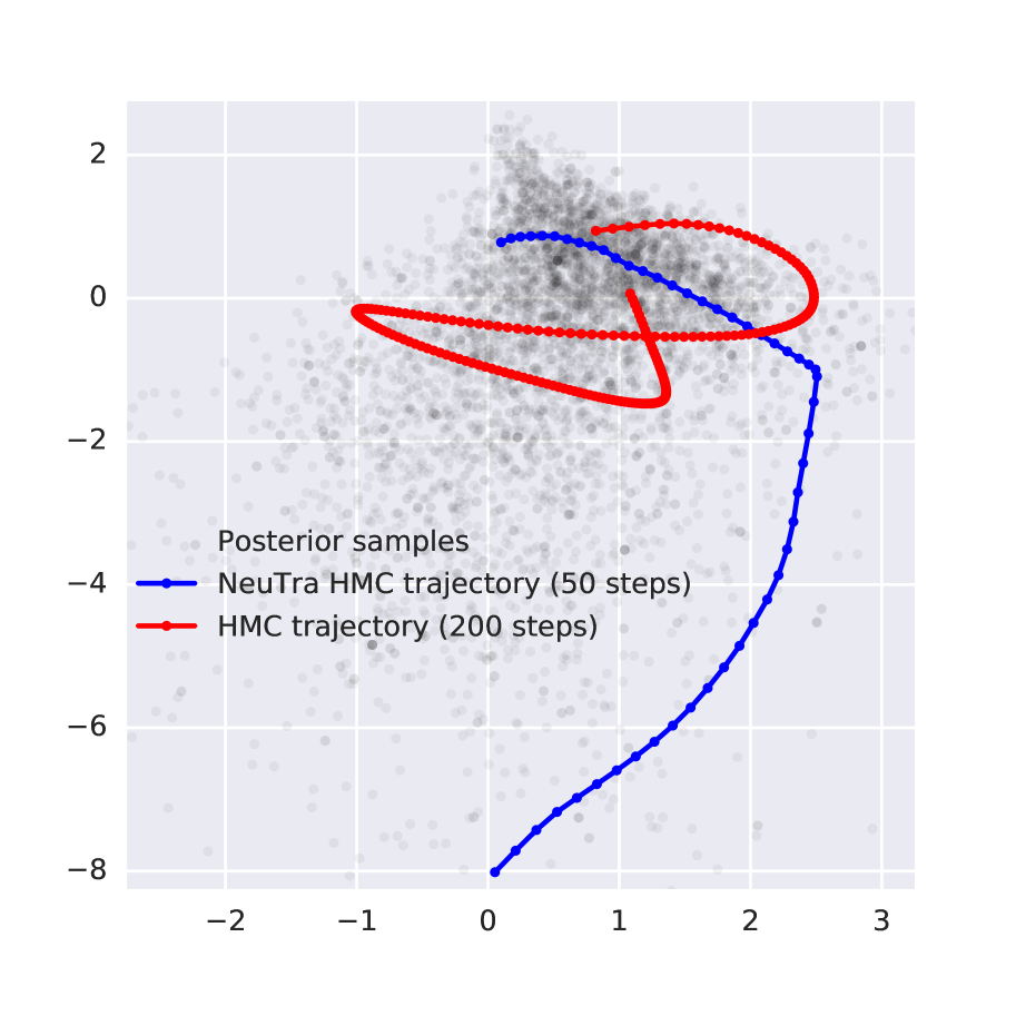
Figure 1 illustrates how simulating Hamiltonian dynamics in the -space defined by an IAF can produce trajectories that quickly explore -space in relatively few steps.
2.3.1 NeuTra in the amortized setting
Amortized variational inference (Kingma & Welling, 2014; Rezende et al., 2014; Gershman & Goodman, 2014) is a popular strategy for learning and inference in latent-variable models. Rather than optimize the parameters of a single variational distribution to minimize the KL divergence to a single posterior , one trains a conditional variational distribution , typically parameterized by a neural network. The cost of fitting can be amortized over many values of .
IAFs and other neural-network-based transport maps are well suited to this sort of strategy; one need only design the network to take some auxiliary inputs as well as the latent vector , or have the base distribution be parameterized by . Since NeuTra HMC is agnostic to how the map was created, it also works in the amortized setting.
3 Related Work
NeuTra HMC has ties to several threads of related work. In this section, we describe some of these connections.
3.1 Riemannian Manifold HMC
Riemannian manifold HMC (RMHMC; Girolami & Calderhead, 2011) tries to speed mixing by accounting for the information geometry of the target distribution. Where HMC generates proposals by simulating Hamiltonian dynamics in Euclidean space, RMHMC simulates Hamiltonian dynamics in a Riemannian space with a position-dependent metric. When this metric is chosen appropriately, RMHMC can make rapid progress in very few steps.
Despite this, RMHMC has some significant downsides compared to standard Euclidean HMC algorithms: since the RMHMC Hamiltonian is non-separable, it requires a more complicated, expensive, and sensitive implicit numerical integrator; the commonly used Fisher metric must be derived by hand for each new model, and is not always available in closed form; if the metric changes rapidly as a function of position, then the integrator may still need to use a small step size; and in high dimensions it may be expensive to compute the metric, its derivatives, its inverse, and its determinant.
Below, we show that the continuous-time dynamics of NeuTra HMC are in fact equivalent to those of RMHMC with a metric defined by the Jacobian of the map. This suggests that NeuTra HMC may be able to achieve many of the benefits of RMHMC with much lower implementation and computational complexity. For example, Figure 1 demonstrates RMHMC-style locally adaptive step size behavior.
Let and . The Hamiltonian defined by NeuTra HMC is
| (5) |
Now, consider the non-separable Hamiltonian that arises if we work in the original -space and define a position-dependent metric :
| (6) |
Now, if we define , then we see that
| (7) |
That is, the Hamiltonians are equivalent. Now, consider the dynamics over implied by :
| (8) |
These are the same as the dynamics implied by :
| (9) |
where we use the fact that .
NeuTra HMC therefore has the potential to deliver speedups comparable to RMHMC without the complications and expense mentioned above. The main downside is that this potential will only be realized if we learn a good explicit map , whereas RMHMC’s metric can be computed from purely local information.
3.2 Learned MCMC Kernels
Classical adaptive MCMC algorithms (Andrieu & Thoms, 2008) try to tune parameters such as step sizes to achieve target acceptance rates or maximize convergence speed (e.g.; Pasarica & Gelman, 2010). More recently, Levy et al. (2018) proposed L2HMC, an adaptive MCMC algorithm to tune a generalization of the leapfrog integrator parameterized by a neural network; like NeuTra, it aims to use powerful models to speed up mixing, but the L2HMC integrator is not symplectic, and therefore may sacrifice some of the leapfrog integrator’s stability over long trajectories (Neal, 2011; Betancourt, 2017). Song et al. (2017) propose a different neural MCMC approach based on adversarial training, although it lacks strong guarantees of convergence. Whereas NeuTra uses a variational approximation to speed up MCMC, Li et al. (2017) propose schemes for using MCMC to improve a variational approximation.
Neal (2011) suggests choosing a covariance matrix for the momenta in HMC based on an estimate of the covariance of the target distribution (or its diagonal), and observes that this corresponds to doing HMC with an identity covariance under a linear change of variables. The Stan software package (Carpenter et al., 2017) adapts this covariance matrix while sampling, effectively tuning a more efficient parameterization. NeuTra goes beyond the linear case.
3.3 Deep Generative Models
A few papers in the deep generative modeling literature have proposed hybrids of variational inference and MCMC. Several (e.g.; Salimans et al., 2015; Zhang et al., 2018; Caterini et al., 2018) have considered using MCMC-based variational bounds to do approximate maximum-likelihood training of variational autoencoders (VAEs). Hoffman (2017) proposed using the standard deviations of a mean-field Gaussian variational distribution to tune per-variable HMC step sizes, which is equivalent to doing HMC under the linear change of variables that makes the variational distribution a standard normal (Neal, 2011). Titsias (2017) proposes a heuristic for training an MCMC transport map by maximizing the log-density of the last sample in the chain; since this method ignores the intractable entropy term bounded by Salimans et al. (2015), it is not clear that it actually encourages mixing as opposed to mode-finding.
4 Experiments
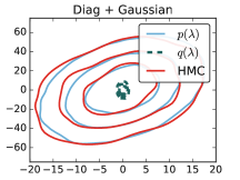
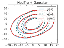
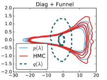
We evaluate NeuTra HMC’s performance on four target distributions: two synthetic problems, sparse logistic regression models applied to the German credit dataset, and a variational autoencoder applied to the MNIST dataset. All experimental code is open-sourced at https://github.com/google-research/google-research/tree/master/neutra.
4.1 Unconditional Target Distributions
Ill-conditioned Gaussian:
In order to test how samplers can handle a highly non-isotropic distribution, we take a dimensional Gaussian distribution with the covariance matrix with eigenvalues sampled from . The covariance matrix is quenched (sampled once and shared among all the experiments). In practice, the eigenvalues range over 6 orders of magnitude.
Neal’s Funnel Distribution:
Sparse logistic regression:
As a non-synthetic example, we consider a hierarchical logistic regression model with a sparse prior applied to the German credit dataset. We use the numeric variant of the dataset, with the covariates standardized to range between -1 and 1. With the addition of a constant factor, this yields 25 covariates.
The model is defined as follows:
| (10) |
where Gam is the Gamma distribution, is the overall scale, are per-dimension scales, are the non-centered covariate weights, denotes the elementwise product of and , and is the sigmoid function. The sparse gamma prior on imposes a soft sparsity prior on the weights, which could be used for variable selection. This parameterization uses D=51 dimensions. We log-transform and to make them unconstrained.
4.1.1 Transport maps and training procedure
For each distribution we consider IAFs with 2 hidden layers per flow, three stacked flows, ELU nonlinearity (Clevert et al., 2015) and hidden dimensionality equal to the target distribution dimensionality. When stacking multiple flows, we reverse the order of dimensions between each flow. We also considered two non-neural maps as baselines: a per-component scale vector (“Diag”) and shift and a lower-triangular affine transformation (“Tril”) and shift. We use the diagonal map as the baseline HMC method, as that approximates the standard practice of basic preconditioning of that method. For sparse logistic regression, we additionally scaled the base Gaussian distribution by 0.1 when training the IAF map.
In all cases, we trained the transport maps with using Adam (Kingma & Ba, 2015) for 5000 steps, starting with a learning rate of 0.01, and decaying it by a factor of 10 at step 1000 and again at step 4000. We used a batch size of 4096 for all problems, running on a Tesla P100 GPU.
4.1.2 HMC sampler hyperparameters
For all HMC experiments we used the corresponding as the initial distribution. In all cases, we ran the 16384 chains for 1000 steps to compute the bias and chain diagnostics, and ran with 4096 chains to compute steps/second.
Without prior information about the target distribution, the standard practice for tuning the HMC step size and number of leapfrog steps is to run multiple pilot runs until acceptable behavior is observed in the chain traces, gross chain statistics and other heuristics. For this work, we automate this process by minimizing:
| (11) |
using Bayesian optimization, where ESS/grad is the effective sample size as defined by Hoffman & Gelman (2011) normalized by the number of target distribution gradient evaluations and is potential scale reduction (Gelman & Rubin, 1992). When computing ESS and we use the per-component second moment rather than the more typical mean as we are interested in how well the HMC chains explore the tails of the target distributions. We compute by starting the chains from our initial distribution which, while convenient, is not the recommended practice as it is underdispersed with respect to the target distribution. The values we obtain should therefore be interpreted as lower bounds. As our distributions have multiple components, we take the maximum and minimum ESS/grad when computing the optimization objective.
The intuition behind Equation 11 is that we want the chains to fully explore the target distribution, leading to a low . Once that is low enough we also want the chains to be efficient by minimizing ESS/grad. In practice, for all the samplers tested all the chain reach an .
When optimizing and we select the step sizes from and number of leapfrog steps from .
4.1.3 Results
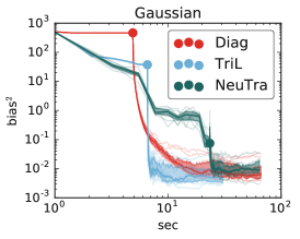
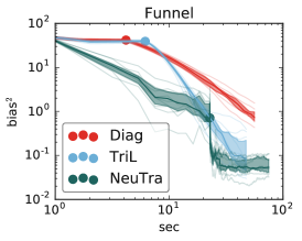
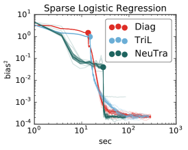
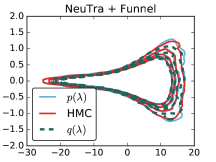
Figure 2 shows samples from the IAF variational distribution as well as the diagonal covariance matrix and the corresponding HMC samples. IAF matches the target distribution very well for both Gaussian and Funnel target distributions, with the remainder taken care of by the NeuTra HMC. The Diag transport map does not match the target distributions all that well, but HMC still manages to recover the target distribution due to its unbiased nature. Note that despite this, HMC has trouble with the neck of the funnel because of the difficult geometry in that region, while NeuTra HMC does better because the transport map has partially simplified that region.
A natural concern about NeuTra HMC is that the time spent training the neural transport map could be instead spent collecting samples from a vanilla HMC sampler. On the other hand, NeuTra HMC might not need as long a warmup (or “burn-in”) period to forget its initialization, firstly because the chains can be initialized with samples from the variational distribution (which has been tuned to be close to the true posterior), and secondly because the chains may mix faster after initialization. Depending on which of these considerations (transport-map training time versus warmup speed) dominates, either NeuTra HMC or vanilla HMC might start generating unbiased samples first.
Figure 3 investigates which of these effects is dominant. We estimated the transient squared bias (averaged across dimensions) when estimating the second moment of each dimension as a function of the wall-clock time. We estimate the bias by averaging across 16384 chains (8x as many variational samples) which gives us a noise floor due to the variance between the chains/samples. For the chains, we discard the first half of the chain as per the standard practice (Angelino et al., 2016).
First, we train the transport map using the variational objective. This objective is not guaranteed to reduce bias depending on the exact relationship between the map parameterization and the target distribution, but we nonetheless observe that it typically does. Critically, when the map is not flexible enough to match the target distribution, estimates based on samples from the variational distribution are biased.
After the distribution is trained, we start the HMC sampling, which asymptotically can reduce the bias to 0 exponentially fast (Angelino et al., 2016). For the Gaussian distribution we observe that HMC with the diagonal preconditioner has trouble converging quickly, although by being so computationally cheap it still overtakes NeuTra by the time it finishes training its IAF. For this distribution the optimal preconditioner is a TriL matrix, so it is not surprising that it performs the best.
For the Funnel the non-neural maps don’t make much progress, and their corresponding chains mix and warm up slowly. NeuTra, on the other hand reaches the noise floor of our bias estimator quickly.
For sparse logistic regresion we observe similar behavior, although the target distribution is well behaved enough for the non-neural transport maps to also reach the noise floor of our bias estimator.
Another way to interpret Figure 3 is as a practitioner’s rule to decide which algorithm to use based on their time and bias requirements. If the bias requirements are not very stringent, the practioner may opt to use a simpler preconditioner which can reach that target level of bias sooner. In fact, for some problems it may be worth to forgo HMC altogether and use the samples from the variational approximation instead, which supports the common choice of that method in many Bayesian learning applications.
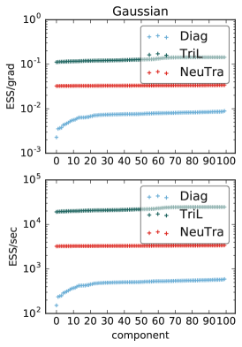
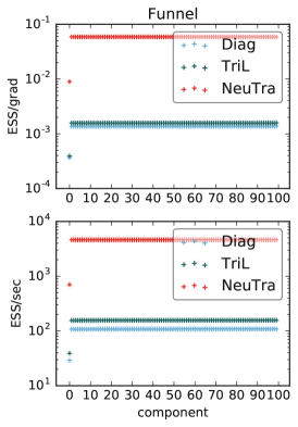
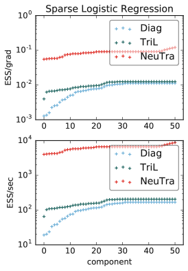
We also investigate the asymptotic behavior of the samplers by measuring the ESS normalized by the number of gradient evaluations and wall-clock duration of a step Figure 4. As before, we look at estimating the second moment of each of the target distribution’s components. In all cases except the Gaussian NeuTra significantly outperforms the non-neural transport maps, often by over an order of magnitude. This is a combination of two effects. First, NeuTra simplifies the target distribution geometry, allowing HMC to explore it more effectively. Second, HMC using non-neural transport maps needs to take many leapfrog steps to reduce the autocorrelation, which may take more wall-clock time than NeuTra even if NeuTra’s neural transport map takes longer per leapfrog step.
4.2 Conditional Target Distributions
Using NeuTra HMC to generate samples from the posterior of a deep latent gaussian model (DLGM) during training is a natural application of our technique. Classically, DLGMs have been trained by constructing an amortized approximate posterior, and then using variational inference to train both the approximate posterior and generative model parameters (Kingma & Welling, 2014; Rezende et al., 2014). More recently, by utilizing neural-net transport maps the quality of the approximate posterior has been improved, yielding higher-quality generative models (Rezende & Mohamed, 2015). To incorporate NeuTra HMC into these models we build upon the interleaved training procedure of Hoffman (2017). The parameters of the approximate posterior and the transport map are trained using the standard ELBO. For each minibatch we initialize the NeuTra HMC chain at the sample from the approximate posterior, and then take a small number of NeuTra HMC steps, taking the final state as the sample used to train the generative model. We use a step size of and leapfrog steps.
| Posterior | |
|---|---|
| Independent Gaussian | |
| IAF | |
| IAF+NeuTra HMC (1 step) | |
| IAF+NeuTra HMC (2 steps) | |
| IAF+NeuTra HMC (4 steps) |
We use the convolutional architecture from Kingma et al. (2016) with the IAF map and train it on dynamically binarized MNIST, reporting the test NLL computed via AIS (20 chains, 10000 interpolation steps) (Wu et al., 2017). Table 1 shows that even a very flexible approximate posterior can be refined via NeuTra HMC. Crucially, no new parameters were added to the model; we simply utilized the IAF transport map used in the standard training procedure. One caveat is that, as reported by Hoffman (2017), training speed is significantly reduced due to the additional evaluations of the model for each leapfrog step.
5 Discussion
We described Neural-Transport (NeuTra) HMC, a method for accelerating Hamiltonian Monte Carlo sampling by nonlinearly warping the geometry of the target distribution using inverse autoregressive flows trained using variational inference. Using IAFs instead of affine flows often dramatically improves mixing speed, especially on posteriors often found in hierarchical Bayesian models.
One remaining concern is that, if the maps fail to adequately capture the geometry of the target distribution, NeuTra could actually slow mixing in the tails. It would be interesting to explore architectures and regularization strategies that could safeguard against this.
References
- Andrieu & Thoms (2008) Andrieu, C. and Thoms, J. A tutorial on adaptive mcmc. Statistics and computing, 18(4):343–373, 2008.
- Angelino et al. (2016) Angelino, E., Johnson, M. J., and Adams, R. P. Patterns of Scalable Bayesian Inference. 2016. ISSN 1935-8237. URL http://arxiv.org/abs/1602.05221.
- Betancourt (2017) Betancourt, M. A conceptual introduction to Hamiltonian MOnte CArlo. arXiv preprint arXiv:1701.02434, 2017.
- Carpenter et al. (2017) Carpenter, B., Gelman, A., Hoffman, M. D., Lee, D., Goodrich, B., Betancourt, M., Brubaker, M., Guo, J., Li, P., and Riddell, A. Stan: A probabilistic programming language. Journal of statistical software, 76(1), 2017.
- Caterini et al. (2018) Caterini, A. L., Doucet, A., and Sejdinovic, D. Hamiltonian variational auto-encoder. arXiv preprint arXiv:1805.11328, 2018.
- Clevert et al. (2015) Clevert, D.-A., Unterthiner, T., and Hochreiter, S. Fast and accurate deep network learning by exponential linear units (elus). In International Conference on Learning Representations, 2015.
- Duane et al. (1987) Duane, S., Kennedy, A. D., Pendleton, B. J., and Roweth, D. Hybrid Monte Carlo. Physics letters B, 195(2):216–222, 1987.
- Gelman & Rubin (1992) Gelman, A. and Rubin, D. B. Inference from iterative simulation using multiple sequences. Statistical Science, 1992.
- Gershman & Goodman (2014) Gershman, S. and Goodman, N. Amortized inference in probabilistic reasoning. In Proceedings of the Annual Meeting of the Cognitive Science Society, 2014.
- Girolami & Calderhead (2011) Girolami, M. and Calderhead, B. Riemann manifold langevin and Hamiltonian Monte Carlo methods. Journal of the Royal Statistical Society: Series B (Statistical Methodology), 73(2):123–214, 2011.
- Hastings (1970) Hastings, W. K. Monte Carlo sampling methods using markov chains and their applications. Biometrika, 57(1):97–109, 1970. doi: 10.1093/biomet/57.1.97. URL http://dx.doi.org/10.1093/biomet/57.1.97.
- Hoffman (2017) Hoffman, M. D. Learning deep latent Gaussian models with Markov chain Monte CArlo. In International Conference on Machine Learning, pp. 1510–1519, 2017.
- Hoffman & Gelman (2011) Hoffman, M. D. and Gelman, A. The no-u-turn sampler: Adaptively setting path lengths in Hamiltonian Monte Carlo. The Journal of Machine Learning Research, 2011.
- Kingma & Ba (2015) Kingma, D. and Ba, J. Adam: A method for stochastic optimization. In International Conference on Learning Representations, 2015.
- Kingma & Welling (2014) Kingma, D. P. and Welling, M. Auto-encoding variational Bayes. International Conference on Learning Representations, 2014.
- Kingma et al. (2016) Kingma, D. P., Salimans, T., and Welling, M. Improving variational inference with inverse autoregressive flow. Advances in Neural Information Processing Systems, (2011):1–8, 2016.
- Levy et al. (2018) Levy, D., Hoffman, M. D., and Sohl-Dickstein, J. Generalizing Hamiltonian Monte Carlo with neural networks. In International Conference on Learning Representations, 2018.
- Li et al. (2017) Li, Y., Turner, R. E., and Liu, Q. Approximate inference with amortised MCMC. arXiv preprint arXiv:1702.08343, 2017.
- Livingstone et al. (2016) Livingstone, S., Betancourt, M., Byrne, S., and Girolami, M. On the geometric ergodicity of Hamiltonian Monte Carlo. arXiv preprint arXiv:1601.08057, 2016.
- Mangoubi & Smith (2017) Mangoubi, O. and Smith, A. Rapid mixing of Hamiltonian Monte Carlo on strongly log-concave distributions. arXiv preprint arXiv:1708.07114, 2017.
- Marzouk et al. (2016) Marzouk, Y., Moselhy, T., Parno, M., and Spantini, A. An introduction to sampling via measure transport. arXiv preprint arXiv:1602.05023, 2016.
- Metropolis et al. (1953) Metropolis, N., Rosenbluth, A. W., Rosenbluth, M. N., Teller, A. H., and Teller, E. Equation of state calculations by fast computing machines. The journal of chemical physics, 21(6):1087–1092, 1953.
- Neal (2003) Neal, R. M. Slice sampling. Annals of Statistics, pp. 705–741, 2003.
- Neal (2011) Neal, R. M. MCMC using Hamiltonian dynamics. In Handbook of Markov Chain MOnte CArlo. CRC Press New York, NY, 2011.
- Parno & Marzouk (2014) Parno, M. and Marzouk, Y. Transport map accelerated markov chain Monte Carlo. arXiv preprint arXiv:1412.5492, 2014.
- Pasarica & Gelman (2010) Pasarica, C. and Gelman, A. Adaptively scaling the metropolis algorithm using expected squared jumped distance. Statistica Sinica, pp. 343–364, 2010.
- Rezende & Mohamed (2015) Rezende, D. and Mohamed, S. Variational Inference with Normalizing Flows. ArXiv e-prints, May 2015.
- Rezende et al. (2014) Rezende, D. J., Mohamed, S., and Wierstra, D. Stochastic backpropagation and approximate inference in deep generative models. In Proceedings of the 31st International Conference on Machine Learning, pp. 1278–1286, 2014.
- Salimans et al. (2015) Salimans, T., Kingma, D., and Welling, M. Markov chain Monte Carlo and variational inference: Bridging the gap. In International Conference on Machine Learning, pp. 1218–1226, 2015.
- Song et al. (2017) Song, J., Zhao, S., and Ermon, S. Generative adversarial learning of markov chains. In ICLR Workshop, 2017.
- Titsias (2017) Titsias, M. K. Learning model reparametrizations: Implicit variational inference by fitting mcmc distributions. arXiv preprint arXiv:1708.01529, 2017.
- Wu et al. (2017) Wu, Y., Burda, Y., Salakhutdinov, R., and Grosse, R. On the quantitative analysis of decoder-based generative models. In International Conference on Learning Representations, 2017.
- Zhang et al. (2018) Zhang, Y., Hernández-Lobato, J. M., and Ghahramani, Z. Ergodic measure preserving flows. arXiv preprint arXiv:1805.10377, 2018.