Active-Learning a Convex Body in Low Dimensions

Abstract

Consider a set $P\subseteq\mathbb{R}^{d}$ of $n$ points, and a convex body $C$ provided via a separation oracle. The task at hand is to decide for each point of $P$ if it is in $C$ using the fewest number of oracle queries. We show that one can solve this problem in two and three dimensions using $O(\varhexagon_{P}\log n)$ queries, where $\varhexagon_{P}$ is the size of the largest subset of points of $P$ in convex position. In 2D, we provide an algorithm that efficiently generates these adaptive queries.

Furthermore, we show that in two dimensions one can solve this problem using $O(\varocircle\left({P,C}\right)\log^{2}n)$ oracle queries, where $\varocircle\left({P,C}\right)$ is a lower bound on the minimum number of queries that any algorithm for this specific instance requires. Finally, we consider other variations on the problem, such as using the fewest number of queries to decide if $C$ contains all points of $P$.

As an application of the above, we show that the discrete geometric median of a point set $P$ in $\mathbb{R}^{2}$ can be computed in $O(n\log^{2}n\,(\log n\log\log n+\varhexagon_{P}))$ expected time.

1 Introduction

1.1 Background

Active learning.

Active learning is a subfield of machine learning. At any time, the learning algorithm is able to query an oracle for the label of a particular data point. One model for active learning is the membership query synthesis model [Ang87]. Here, the learner wants to minimize the number of oracle queries, as such queries are expensive—they usually correspond to either consulting with a specialist, or performing an expensive computation. In this setting, the learning algorithm is allowed to query the oracle for the label of any data point in the instance space. See [Set09] for a more in-depth survey on the various active learning models.

Figure 1.1: The shaded region shows the symmetric difference between the hypothesis and true classifier. (I) Learning halfspaces. (II) Learning arbitrary convex regions.

PAC learning.

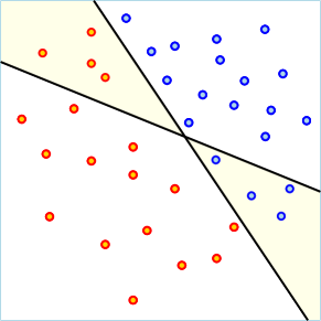
A classical approach for learning is using random sampling, where one gets labels for the samples (i.e., in the above setting, the oracle is asked for the labels of all items in the random sample). PAC learning studies the size of the sample needed. For example, consider the problem of learning a halfplane for $n$ points $P\subset\mathbb{R}^{2}$, given a parameter $\varepsilon\in(0,1)$. The first stage is to take a labeled random sample $R\subseteq P$. The algorithm computes any halfplane that classifies the sample correctly (i.e., the hypothesis). The misclassified points lie in the symmetric difference between the learned halfplane, and the (unknown) true halfplane, see Figure 1.1. In this case, the error region is a double wedge, and it is well known that its VC-dimension [VC71] is a constant (at most eight). As such, by the $\varepsilon$-net Theorem [HW87], a sample of size $O(\varepsilon^{-1}\log\varepsilon^{-1})$ is an $\varepsilon$-net for double wedges, which implies that this random sampling algorithm has at most $\varepsilon n$ error.

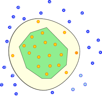
A classical example of a hypothesis class that cannot be learned is the set of convex regions (even in the plane). Indeed, given a set of points $P$ in the plane, any sample $R\subseteq P$ cannot distinguish between the true region being ${\mathcal{CH}}\left({R}\right)$ or ${\mathcal{CH}}\left({P}\right)$. Intuitively, this is because the hypothesis space in this case grows exponentially in the size of the sample (instead of polynomially). See Figure 1.2.

Figure 1.2:

We stress that the above argument does not necessarily imply these types of hypothesis classes are unlearnable in practice. In general, there are other ways for learning algorithms to handle hypothesis classes with high (or even infinite) VC-dimension (for example, using regularization or assuming there is a large margin around the decision boundary).

Weak $\varepsilon$-nets.

Because $\varepsilon$-nets for convex ranges do not exist, an interesting direction to overcome this problem is to define weak $\varepsilon$-nets [HW87]. A set of points $R$ in the plane, not necessarily a subset of $P$, is a weak $\varepsilon$-net for $P$ if for any convex body $C$ containing at least $\varepsilon n$ points of $P$, it also contains a point of $R$. Matoušek and Wagner [MW03] gave a weak $\varepsilon$-net construction of size $O(\varepsilon^{-d}(\log\varepsilon^{-1})^{O(d^{2}\log d)})$, which is doubly exponential in the dimension. The state of the art is the recent result of Rubin [Rub18], that shows a weak $\varepsilon$-net construction in the plane of size (roughly) $O(1/\varepsilon^{3/2})$. However, these weak $\varepsilon$-nets cannot be used for learning such concepts. Indeed, the analysis above required an $\varepsilon$-net for the symmetric difference of two convex bodies of finite complexity, see Figure 1.1.

PAC learning with additional parameters.

If one assumes the input instance obeys some additional structural properties, then random sampling can be used. For example, suppose that the point set $P$ has at most $k$ points in convex position. For an arbitrary convex body $C$, the convex hull ${\mathcal{CH}}\left({P\cap C}\right)$ has complexity at most $k$. Let $R\subseteq P$ be a random sample, and $C^{\prime}$ be the learned classifier for $R$. The region of error is the symmetric difference between $C$ and $C^{\prime}$. In particular, since $k$-vertex polytopes in $\mathbb{R}^{d}$ have VC-dimension bounded by $O(d^{2}k\log k)$ [Kup20], this implies that the error region also has VC-dimension at most $O(d^{2}k\log k)$. Hence if $R$ is a random sample of size $O(d^{2}k\log k\varepsilon^{-1}\log\varepsilon^{-1})$, the $\varepsilon$-net Theorem [HW87] implies that this sampling algorithm has error at most $\varepsilon n$. However, even for a set of $n$ points chosen uniformly at random from the unit square $[0,1]^{2}$, the expected number of points in convex position is $O(n^{1/3})$ [AB09]. Since we want $\left|{R}\right|<n$, this random sampling technique is only useful when $\varepsilon$ is larger than $\log^{2}n/n^{2/3}$ (ignoring constants).

To summarize the above discussions, random sampling on its own does not seem powerful enough to learn arbitrary convex bodies, even if one allows some error to be made. In this paper we focus on developing algorithms for learning convex bodies in low dimensions, where the algorithms are deterministic and do not make any errors.

Figure 1.3: (I) A set of points $P$. (II) The unknown convex body $C$. (III) Classifying all points of $P$ as either inside or outside $C$.

1.2 Problem and motivation

The problem.

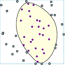
In this paper, we consider a variation on the active learning problem, in the membership query synthesis model. Suppose that the learner is trying to learn an unknown convex body $C$ in $\mathbb{R}^{d}$. Specifically, the learner is provided with a set $P$ of $n$ unlabelled points in $\mathbb{R}^{d}$, and the task is to label each point as either inside or outside $C$, see Figure 1.3. For a query $q\in\mathbb{R}^{d}$, the oracle either reports that $q\in C$, or returns a hyperplane separating $q$ and $C$ (as a proof that $q\not\in C$). Note that if the query is outside the body, the oracle answer is significantly more informative than just the label of the point. The problem is to minimize the overall number of queries performed.

Hard and easy instances.

Note that in the worst case, an algorithm may have to query the oracle for all input points—such a scenario happens when the input points are in convex position, and any possible subset of the points can be the points in the (appropriate) convex body. As such, the purpose here is to develop algorithms that are instance sensitive—if the given instance is easy, they work well. If the given instance is hard, they might deteriorate to the naive algorithm that queries all points.

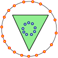
Natural inputs where one can hope to do better, are when relatively few points are in convex position. Such inputs are grid points, or random point sets, among others. However, there are natural instances of the problem that are easy, despite the input having many points in convex position. For example, consider when the convex body is a triangle, with the input point set being $n/2$ points spread uniformly on a tiny circle centered at the origin, while the remaining $n/2$ points are outside the convex body, spread uniformly on a circle of radius $10$ centered at the origin, see Figure 1.4. Clearly, such a point set can be fully classified using a sequence of a constant number of oracle queries. See Figure 3.1 for some related examples.

Figure 1.4:

Discretely optimizing convex functions.

As an application of this particular query model, we explore the connection between active-learning a convex body and minimizing a convex function. Concretely, suppose we are given a set of $n$ points $P$ in the plane and a convex function $f:\mathbb{R}^{2}\to\mathbb{R}$ equipped with an oracle that can evaluate $f$ or the derivative of $f$ at a given point. Our goal is to compute the point in $P$ minimizing $\min_{p\in P}f(p)$ using the fewest number of oracle queries (i.e., evaluations of $f$ or the derivative). We discuss the result in full in Section 5.

We show that there is a natural connection between the studied query model and this problem. Namely, the level sets of a convex function are convex bodies, and the gradient of $f$ can be used to construct separating lines for the level set. Thus, developing algorithms for active-learning a convex body in the membership query synthesis model in conjunction with the two aforementioned facts leads to alterative methods for minimizing a convex function over a discrete collection of points. Importantly, the running time of such algorithms depend not only on how quickly we can evaluate $f$, but also on the structure of the point set $P$, as we aim to develop instance sensitive algorithms.

1.3 Additional motivation & previous work

Separation oracles.

The use of separation oracles is a common tool in optimization (e.g., solving exponentially large linear programs) and operations research. It is natural to ask what other problems can be solved efficiently when given access to this specific type of oracle. For example, Bárány and Füredi [BF87] study the problem of computing the volume of a convex body in $\mathbb{R}^{d}$ given access to a separation oracle.

Other types of oracles.

Various models of computation utilizing oracles have been previously studied within the computational geometry community. Examples of other models include nearest-neighbor oracles (i.e., black-box access to nearest neighbor queries over a point set $P$) [HKMR16], proximity probes (in which given a convex polygon $C$ and a query $q$, returns the distance from $q$ to $C$) [PASG13], and linear queries. Recently, Ezra and Sharir [ES19] gave an improved algorithm for the problem of point location in an arrangement of hyperplanes. Here, a linear query consists of a point $x$ and a hyperplane $h$, and outputs either that $x$ lies on $h$, or else the side of $h$ contains $x$. Alternatively, their problem can be interpreted as querying whether or not a given point lies in a halfspace $h^{+}$. Here, we study the more general problem as the convex body can be the intersection of many halfspaces.

Furthermore, other types of active learning models (in addition to the membership query model) have also been studied within the learning community, see, for example, [Ang87].

Active learning.

As discussed, the problem at hand can be interpreted as active-learning a convex body in relation to a set of points $P$ that need to be classified (as either inside or outside the body), where the queries are via a separation oracle. We are unaware of any work directly on this problem in the computational geometry community, while there is some work in the learning community that studies related active-learning classification problems [CAL94, GG07, Set09, KLMZ17].

For example, Kane et al. [KLMZ17] study the problem of actively learning halfspaces with access to comparison queries. Given a halfspace $h^{+}$ to learn, the model has two types of queries: (i) label queries (given $x\in\mathbb{R}^{d}$, is $x\in h^{+}$?), and (ii) comparison queries (given $x_{1},x_{2}\in\mathbb{R}^{d}$, is $x_{1}$ closer to the boundary of $h^{+}$ than $x_{2}$?). For example, they show that in the plane, one can classify all points using $O(\log n)$ comparison/label queries in expectation.

1.4 Our results

1. We develop a greedy algorithm, for points in the plane, that solves the problem using $O(\varhexagon_{P}\log n)$ oracle queries, where $\varhexagon_{P}$ is the size of the largest subset of points of $P$ in convex position. See Theorem 2.8. It is known that for a random set of $n$ points in the unit square, $\mathop{\mathbf{E}}\!\left[{\varhexagon_{P}}\right]=\Theta(n^{1/3})$ [AB09], which readily implies that classifying these points can be solved using $O(n^{1/3}\log n)$ oracle queries. A similar bound holds for the $\sqrt{n}\times\sqrt{n}$ grid. An animation of this algorithm is on YouTube [HJR18]. We also show that this algorithm can be implemented efficiently, using dynamic segment trees, see Lemma 2.9.

   We remark that Kane et al. [KLMZ17] develop a framework and randomized algorithm for learning a concept $C$, where the expected number of queries depends near-linearly on a parameter they define as the inference dimension [KLMZ17, Definition III.1] of the concept class. For our problem, one can show that the inference dimension is $O(\varhexagon_{P})$. As a corollary of their framework, one can obtain a randomized algorithm that solves our problem where the expected number of queries is $O(\varhexagon_{P}\log n)$, which matches the performance of our deterministic algorithm. See Section 2.2.5 for details.

2. The above algorithm naturally extends to three dimensions, also using $O(\varhexagon_{P}\log n)$ oracle queries. While the proof idea is similar to that of the algorithm in 2D, we believe the analysis in three dimensions is also technically interesting. See Theorem 2.19.

3. For a given point set $P$ and convex body $C$, we define the separation price $\varocircle\left({P,C}\right)$ of an instance $(P,C)$, and show that any algorithm classifying the points of $P$ in relation to $C$ must make at least $\varocircle\left({P,C}\right)$ oracle queries (Lemma 3.1).

   As an aside, we show that when $P$ is a set of $n$ points chosen uniformly at random from the unit square and $C$ is a (fixed) smooth convex body, $\mathop{\mathbf{E}}\!\left[{\varocircle\left({P,C}\right)}\right]=O(n^{1/3})$, and this bound is tight when $C$ is a disk (our result also generalizes to higher dimensions, see Lemma A.3). For randomly chosen points, the separation price is related to the expected size of the convex hull of $P\cap C$, which is also known to be $\Theta(n^{1/3})$ [Wei07]. We believe this result may be of independent interest, see Appendix A.

4. In Section 3 we present an improved algorithm for the 2D problem, and show that the number of queries made is $O(\varocircle\left({P,C}\right)\log^{2}n)$. This result is $O(\log^{2}n)$ approximation to the optimal solution, see Theorem 3.7.

5. We consider the extreme scenarios of the problem: Verifying that all points are either inside or outside of $C$. For each problem we present a $O(\log n)$ approximation algorithm to the optimal strategy. The results are presented in Section 4, see Lemma 4.2 and Lemma 4.4.

6. Section 5 presents an application of the above results, we consider the problem of minimizing a convex function $f:\mathbb{R}^{2}\to\mathbb{R}$ over a point set $P$. Specifically, the goal is to compute $\arg\min_{p\in P}f(p)$. If $f$ and its derivative can be efficiently evaluated at a given query point, then $f$ can be minimized over $P$ using $O(\varhexagon_{P}\log^{2}n)$ queries to $f$ (or its derivative) in expectation. We refer the reader to Lemma 5.5.

   Given a set of $n$ points $P$ in $\mathbb{R}^{d}$, the discrete geometric median of $P$ is a point $p\in P$ minimizing the function $\sum_{q\in P}\|p-q\|_{2}$. As a corollary of Lemma 5.5, we obtain an algorithm for computing the discrete geometric median for $n$ points in the plane. The algorithm runs in $O(n\log^{2}n\cdot(\log n\log\log n+\varhexagon_{P}))$ expected time. See Lemma 5.6. In particular, if $P$ is a set of $n$ points chosen uniformly at random from the unit square, it is known that $\mathop{\mathbf{E}}\!\left[{\varhexagon_{P}}\right]=\Theta(n^{1/3})$ [AB09] and hence the discrete geometric median can be computed in $O(n^{4/3}\log^{2}n)$ expected time.

   While there has been ample work on approximating the geometric median (recently, Cohen et al. [CLM+16] gave a $(1+\varepsilon)$-approximation algorithm to the geometric median in $O(dn\log^{3}(1/\varepsilon))$ time), we are unaware of any exact sub-quadratic algorithm for the discrete case even in the plane.

Throughout this paper, the model of computation we have assumed is unit-cost real RAM.

2 The greedy algorithm in two and three dimensions

2.1 Preliminaries

For a set of points $P\subseteq\mathbb{R}^{2}$, let ${\mathcal{CH}}\left({P}\right)$ denote the convex hull of $P$. Given a convex body $C\subseteq\mathbb{R}^{d}$, two points $p,x\in\mathbb{R}^{d}\setminus\mathrm{int}\left({C}\right)$ are mutually visible, if the segment $px$ does not intersect $\mathrm{int}\left({C}\right)$, where $\mathrm{int}\left({C}\right)$ is the interior of $C$. We also use the notation $P\cap C=\left\{p\in P\;\middle|\;p\in C\right\}$.

For a point set $P\subseteq\mathbb{R}^{d}$, a centerpoint of $P$ is a point $\mathcalb{c}\in\mathbb{R}^{d}$, such that for any closed halfspace $h^{+}$ containing $\mathcalb{c}$, we have $\left|{h^{+}\cap P}\right|\geq\left|{P}\right|/(d+1)$. A centerpoint always exists, and it can be computed exactly in $O(n^{d-1}+n\log n)$ time [Cha04].

Let $C$ be a convex body in $\mathbb{R}^{d}$ and $q\in\mathbb{R}^{d}$ be a point such that $q$ lies outside $C$. A hyperplane $h$ separates $q$ from $C$ if $q$ lies in the closed halfspace $h^{+}$ bounded by $h$, and $C$ is contained in the open halfspace $h^{-}$ bounded by $h$. This definition allows the separating hyperplane to contain the point $q$, and will simplify the descriptions of the algorithms.

2.2 The greedy algorithm in 2D

Given a set of points $P$ in $\mathbb{R}^{2}$ and a convex body $C$ specified via a separation oracle, recall that the problem is to classify, for all the points of $P$, whether or not they are in $C$, using the fewest oracle queries possible. We define some operations the algorithm will use before stating the algorithm in full. Finally, we analyze the the number of queries the algorithm performs.

2.2.1 Operations

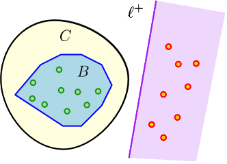
Initially, the algorithm copies $P$ into a set $U$ of unclassified points. The algorithm is going to maintain an inner approximation $B\subseteq C$. There are two types of updates (Figure 2.1 illustrates the two operations):

1. expand$(p)$: Given a point $p\in C\setminus B$, the algorithm is going to:

   1. Update the inner approximation: $B\leftarrow{\mathcal{CH}}\left({B\cup\left\{{p}\right\}}\right)$.

   2. Remove (and mark) newly covered points: $U\leftarrow U\setminus B$.

2. remove$(\mathcalb{l})$: Given a closed halfplane $\mathcalb{l}^{+}$ such that $\mathrm{int}\left({C}\right)\cap\mathcalb{l}^{+}=\emptyset$, the algorithm marks all the points of $U{l}=U\cap\mathrm{int}\left({\mathcalb{l}^{+}}\right)$ as being outside $C$, and sets $U\leftarrow U\setminus U{l}$.

Figure 2.1: (I) Performing ${{\color[rgb]{0.59,0,0.66}\texttt{\bf{expand}}}}{}(p)$, and marking points inside $C$. (II) Performing ${{\color[rgb]{0.59,0,0.66}\texttt{\bf{remove}}}}{}(\mathcalb{l})$, and marking points outside $C$.

2.2.2 The algorithm

The algorithm repeatedly performs rounds, as described next, until the set of unclassified points is empty.

At every round, if the inner approximation $B$ is empty, then the algorithm sets $U^{+}=U$. Otherwise, the algorithm picks a line $\mathcalb{l}$ that is tangent to $B$ with the largest number of points of $U$ on the other side of $\mathcalb{l}$ than $B$. Let $\mathcalb{l}^{-}$ and $\mathcalb{l}^{+}$ be the two closed halfspace bounded by $\mathcalb{l}$, where $B\subseteq\mathcalb{l}^{-}$. The algorithm computes the point set $U^{+}=U\cap\mathcalb{l}^{+}$. We have two cases:

1. Suppose $\left|{U^{+}}\right|$ is of constant size. The algorithm queries the oracle for the status of each of these points. For every point $p\in U^{+}$, such that $p\in C$, the algorithm performs expand$(p)$. Otherwise, the oracle returned a separating line $\mathcalb{l}$, and the algorithm calls remove$(\mathcalb{l}^{+})$.

2. Otherwise, $\left|{U+}\right|$ does not have constant size. The algorithm computes a centerpoint $\mathcalb{c}\in\mathbb{R}^{2}$ for $U^{+}$, and asks the oracle for the status of $\mathcalb{c}$. There are two possibilities:

   1. If $\mathcalb{c}\in C$, then the algorithm performs expand$(\mathcalb{c})$.

   2. If $\mathcalb{c}\notin C$, then the oracle returned a separating line $\mathcalb{h}$, and the algorithm performs remove$(\mathcalb{h})$.

2.2.3 Analysis

Let $B_{i}$ be the inner approximation at the start of the $i$th iteration, and let $z$ be the first index where $B_{z}$ is not an empty set. Similarly, let $U_{i}$ be the set of unclassified points at the start of the $i$th iteration, where initially $U_{1}=U$.

Lemma 2.1.

The number of (initial) iterations in which the inner approximation is empty is $z=O(\log n)$.

Proof:

As soon as the oracle returns a point that is in $C$, the inner approximation is no longer empty. As such, we need to bound the initial number of iterations where the oracle returns that the query point is outside $C$. Let $f_{i}=\left|{U_{i}}\right|$, and note that $U_{1}=P$ and $f_{1}=\left|{P}\right|=n$. Let $\mathcalb{c}_{i}$ be the centerpoint of $U_{i}$, which is the query point in the $i$th iteration ($\mathcalb{c}_{i}$ is outside $C$). As such, the line separating $\mathcalb{c}_{i}$ from $C$, returned by the oracle, has at least $f_{i}/3$ points of $U_{i}$ on the same side as $\mathcalb{c}_{i}$, by the centerpoint property. All of these points get labeled in this iteration, and it follows that $f_{i+1}\leq(2/3)f_{i}$, which readily implies the claim, since $f_{z}<1$, for $z=\left\lceil{\log_{3/2}n}\right\rceil+1$.  

Definition 2.2 (Visibility graph).

Consider the graph $G_{i}$ over $U_{i}$, where two points $p,r\in U_{i}$ are connected $\iff$ the segment $pr$ does not intersect the interior of $B_{i}$.

Figure 2.2: Four points and a convex body with their associated circular intervals.

The visibility graph as an interval graph.

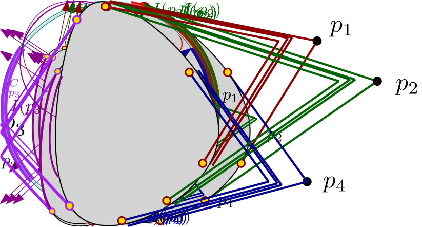
For a point $p\in U_{i}$, let $I_{i}(p)$ be the set of all directions $v$ (i.e., vectors of length $1$) such that there is a line perpendicular to $v$ that separates $p$ from $B_{i}$. Formally, a line $\mathcalb{l}$ separates $p$ from $B_{i}$, if the interior of $B_{i}$ is on one side of $\mathcalb{l}$ and $p$ is on the (closed) other side of $\mathcalb{l}$ (if $p\in\mathcalb{l}$, the line is still considered to separate the two). Clearly, $I_{i}(p)$ is a circular interval on the unit circle. See Figure 2.2. The resulting set of intervals is $\mathcal{V}_{i}=\left\{I_{i}(p)\;\middle|\;p\in U_{i}\right\}$. It is easy to verify that the intersection graph of $\mathcal{V}_{i}$ is $G_{i}$. Throughout the execution of the algorithm, the inner approximation $B_{i}$ grows monotonically, this in turn implies that the visibility intervals shrink over time; that is, $I_{i}(p)\subseteq I_{i-1}(p)$, for all $p\in P$ and $i$. Intuitively, in each round, either many edges from $G_{i}$ are removed (because intervals had shrunk and they no longer intersect), or many vertices are removed (i.e., the associated points are classified).

Definition 2.3.

Given a set $\mathcal{V}$ of objects (e.g., intervals) in a domain ${D}$ (e.g., unit circle), the depth of a point $p\in D$, is the number of objects in $\mathcal{V}$ that contain $p$. Let $\mathrm{depth}\left({\mathcal{V}}\right)$ be the maximum depth of any point in ${D}$.

When it is clear, we use $\mathrm{depth}\left({G}\right)$ to denote $\mathrm{depth}\left({\mathcal{V}}\right)$, where $G=(\mathcal{V},E)$ is the intersection graph of the intervals $\mathcal{V}$ as defined above. Throughout, we commonly refer to $G$ as the intersection graph.

First, we bound the number of edges in this visibility graph $G$ and then argue that in each iteration, either many edges of $G$ are discarded or vertices are removed (as they are classified).

Lemma 2.4.

Let $\mathcal{V}$ be a set of $n$ intervals on the unit circle, and let $G=(\mathcal{V},E)$ be the associated intersection graph. Then $\left|{E}\right|=O(\alpha\omega^{2})$, where $\omega=\mathrm{depth}\left({\mathcal{V}}\right)$ and $\alpha=\alpha(G)$ is the size of the largest independent set in $G$. Furthermore, the upper bound on $\left|{E}\right|$ is tight.

Proof:

Let $J$ be the largest independent set of intervals in $G$. The intervals of $J$ divide the circle into $2\left|{J}\right|$ (atomic) circular arcs. Consider such an arc $\gamma$, and let $K(\gamma)$ be the set of all intervals of $\mathcal{V}$ that are fully contained in $\gamma$. All the intervals of $K(\gamma)$ are pairwise intersecting, as otherwise one could increase the size of the independent set. As such, all the intervals of $K(\gamma)$ must contain a common intersection point. It follows that $\left|{K(\gamma)}\right|\leq\omega$.

Let $K^{\prime}(\gamma)$ be the set of all intervals intersecting $\gamma$. This set might contain up to $2\omega$ additional intervals (that are not contained in $\gamma$), as each such additional interval must contain at least one of the endpoints of $\gamma$. Namely, $\left|{K^{\prime}(\gamma)}\right|\leq 3\omega$. In particular, any two intervals intersecting inside $\gamma$ both belong to $K^{\prime}(\gamma)$. As such, the total number of edges contributed by $K^{\prime}(\gamma)$ to $G$ is at most $\binom{3\omega}{2}=O(\omega^{2})$. Since there are at most $2\alpha$ arcs under consideration, the total number of edges in $G$ is bounded by $O(\alpha\omega^{2})$, which implies the claim.

The lower bound is easy to see by taking an independent set of intervals of size $\alpha$, and replicating every interval $\omega$ times.  

Lemma 2.5.

Let $P$ be a set of $n$ points in the plane lying above the $x$-axis, $\mathcalb{c}$ be a centerpoint of $P$, and $S=\binom{P}{2}$ be set of all segments induced by $P$. Next, consider any point $r$ on the $x$-axis. Then, the segment $\mathcalb{c}r$ intersects at least $n^{2}/36$ segments of $S$.

Proof:

If the segment $\mathcalb{c}r$ intersects the segment $p_{1}p_{2}$, for $p_{1},p_{2}\in P$, then we consider $p_{1}$ and $p_{2}$ to no longer be mutually visible. It suffices to lower bound the number of pairs of points that lose mutual visibility of each other.

Figure 2.3:

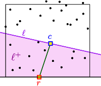
Consider a line $\mathcalb{l}$ passing through the point $\mathcalb{c}$, see Figure 2.3.. Let $\mathcalb{l}^{+}$ be the closed halfspace bounded by $\mathcalb{l}$ containing $r$. Note that $\left|{P\cap\mathcalb{l}^{+}}\right|\geq n/3$, since $\mathcalb{c}$ is a centerpoint of $P$, and $\mathcalb{c}\in\mathcalb{l}$. Rotate $\mathcalb{l}$ around $\mathcalb{c}$ until there are $\geq n/6$ points on each side of $r\mathcalb{c}$ in the halfspace $\mathcalb{l}^{+}$. To see why this rotation of $\mathcalb{l}$ exists, observe that the two halfspaces bounded by the line spanning $r\mathcalb{c}$, have zero points on one side, and at least $n/3$ points on the other side — a continuous rotation of $\mathcalb{l}$ between these two extremes, implies the desired property.

Observe that points in $\mathcalb{l}^{+}$ and on opposite sides of the segment $\mathcalb{c}r$ cannot see each other, as the segment connecting them must intersect $\mathcalb{c}r$. Consequently, the number of induced segments that $\mathcalb{c}r$ intersects is at least $n^{2}/36$.  

For a graph $G$, we let $E\left({G}\right)$ denote the set of edges in $G$, and let $\left|{E\left({G}\right)}\right|$ denote the number of edges in $G$.

Lemma 2.6.

Let $G_{i}$ be the intersection graph, in the beginning of the $i$th iteration, and let $m_{i}=\left|{E\left({G_{i}}\right)}\right|$. After the $i$th iteration of the greedy algorithm, we have $m_{i+1}\leq m_{i}-\omega^{2}/36$, where $\omega=\mathrm{depth}\left({G_{i}}\right)$.

Proof:

Recall that in the algorithm $U^{+}=U_{i}\cap\mathcalb{l}^{+}$ is the current set of unclassified points and $\mathcalb{l}$ is the line tangent to $B_{i}$, where $\mathcalb{l}^{+}$ is the closed halfspace that avoids the interior of $B_{i}$ and contains the largest number of unlabeled points of $U_{i}$. We have that $\omega=\left|{U^{+}}\right|$.

If a remove operation was performed in the $i$th iteration, then the number of points of $U^{+}$ that are discarded is at least $\omega/3$. In this case, the oracle returned a separating line $\mathcalb{h}$ between a centerpoint $\mathcalb{c}$ of $U^{+}$ and the inner approximation. For the halfspace $\mathcalb{h}^{+}$ containing $\mathcalb{c}$, we have $t_{i}=\left|{U^{+}\cap\mathcalb{h}^{+}}\right|\geq\left|{U^{+}}\right|/3\geq\omega/3$. Furthermore, all the points of $U^{+}$ are pairwise mutually visible (in relation to the inner approximation $B_{i}$). Namely,

$$m_{i+1}=\left|{E\left({G_{i}-(U^{+}\cap\mathcalb{h}^{+})}\right)}\right|\leq m_{i}-\binom{t_{i}}{2}\leq m_{i}-\omega^{2}/36.$$

If an expand operation was performed, the centerpoint $\mathcalb{c}$ of $U^{+}$ is added to the current inner approximation $B_{i}$. Let $r$ be a point in $\mathcalb{l}\cap B_{i}$, and let $\mathcalb{c}_{i}$ be the centerpoint of $U_{i}$ computed by the algorithm. By Lemma 2.5 applied to $r,\mathcalb{c}$ and $U^{+}$, we have that at least $\omega^{2}/36$ pairs of points of $U^{+}$ are no longer mutually visible to each other in relation to $B_{i+1}$. We conclude, that at least $\omega^{2}/36$ edges of $G_{i}$ are no longer present in $G_{i+1}$.  

Definition 2.7.

A subset of points $X\subseteq P\subseteq\mathbb{R}^{2}$ are in convex position, if all the points of $X$ are vertices of ${\mathcal{CH}}\left({X}\right)$ (note that a point in the middle of an edge is not considered to be a vertex). The index of $P$, denoted by $\varhexagon_{P}$, is the cardinality of the largest subset of $P$ of points that are in convex position.

Theorem 2.8.

Let $C$ be a convex body provided via a separation oracle, and let $P$ be a set of $n$ points in the plane. The greedy classification algorithm performs $O\bigl{(}(\varhexagon_{P}+1)\log n\bigr{)}$ oracle queries. The algorithm correctly identifies all points in $P\cap C$ and $P\setminus C$.

Proof:

By Lemma 2.1, the number of iterations (and also queries) in which the inner approximation is empty is $O(\log n)$, and let $z=O(\log n)$ be the first iteration such that the inner approximation is not empty. It suffices to bound the number of queries made by the algorithm after the inner approximation becomes non-empty.

For $i\geq z$, let $G_{i}=(U_{i},E_{i})$ denote the visibility graph of the remaining unclassified points $U_{i}$ in the beginning of the $i$th iteration. Any independent set in $G_{i}$ corresponds to a set of points $X\subseteq P$ that do not see each other due to the presence of the inner approximation $B_{i}$. That is, $X$ is in convex position, and furthermore $\left|{X}\right|\leq\varhexagon_{P}$.

For $0\leq t\leq n$, let $s\left({t}\right)$ be the first iteration $i$, such that $\mathrm{depth}\left({G_{i}}\right)\leq t$. Since the depth of $G_{i}$ is a monotone decreasing function, this quantity is well defined. An epoch is a range of iterations between $s(t)$ and $s(t/2)$, for any parameter $t$. We claim that an epoch lasts $O(\varhexagon_{P})$ iterations (and every iteration issues only one oracle query). Since there are only $O(\log n)$ (non-overlapping) epochs till the algorithm terminates, as the depth becomes zero, this implies the claim.

So consider such an epoch starting at $i=s\left({t}\right)$. We have $m=m_{i}=\left|{E\left({G_{i}}\right)}\right|=O(\varhexagon_{P}t^{2})$, by Lemma 2.4, since $\varhexagon_{P}$ is an upper bound on the size of the largest independent set in $G_{i}$. By Lemma 2.6, as long as the depth of the intervals is at least $t/2$, the number of edges removed from the graph at each iteration, during this epoch, is at least $\Omega(t^{2})$. As such, the algorithm performs at most $O(m_{i}/t^{2})=O(\varhexagon_{P})$ iterations in this epoch, till the maximum depth drops to $t/2$.  

2.2.4 Implementing the greedy algorithm

With the use of dynamic segment trees [MN90] we show that the greedy classification algorithm can be implemented efficiently.

Lemma 2.9.

Let $C$ be a convex body provided via a separation oracle, and let $P$ be a set of $n$ points in the plane. If an oracle query costs time $T$, then the greedy algorithm can be implemented in $O\bigl{(}n\log^{2}n\log\log n+T\cdot\varhexagon_{P}\log n\bigr{)}$ expected time.

Proof:

The algorithm follows the proof of Theorem 2.8. We focus on efficiently implementing the algorithm once inner approximation is no longer empty. Let $U\subseteq P$ be the subset of unclassified points. By binary searching on the vertices of the inner approximation $B$, we can compute the collection of visibility intervals $\mathcal{V}$ for all points in $U$ in $O(\left|{U}\right|\log m)=O(n\log n)$ time (recall that $\mathcal{V}$ is a collection of circular intervals on the unit circle). We store these intervals in a dynamic segment tree $\mathcal{T}$ with the modification that each node $v$ in $\mathcal{T}$ stores the maximum depth over all intervals contained in the subtree rooted at $v$. Note that $\mathcal{T}$ can be made fully dynamic to support updates in $O(\log n\log\log n)$ time [MN90].

An iteration of the greedy algorithm proceeds as follows. Start by collecting all points $U^{+}\subseteq U$ realizing the maximum depth using $\mathcal{T}$. When $t=\left|{U^{+}}\right|$, this step can be done in $O(\log n+t)$ time by traversing $\mathcal{T}$. We compute the centerpoint of $U^{+}$ in $O(t\log t)$ expected time [Cha04] and query the oracle using this centerpoint. Either points of $U$ are classified (and we delete their associated intervals from $\mathcal{T}$) or we improve the inner approximation. The inner approximation (which is the convex hull of query points inside the convex body $C$) can be maintained in an online fashion with insert time $O(\log n)$ [PS85, Chapter 3]. When the inner approximation expands, the points of $U^{+}$ have their intervals shrink. As such, we recompute $I(p)$ for each $p\in U^{+}$ and reinsert $I(p)$ into $\mathcal{T}$.

As defined in the proof of Theorem 2.8, an epoch is the subset of iterations in which the maximum depth is in the range $[t/2,t]$, for some integer $t$. During such an epoch, we make two claims:

1. there are $\sigma=O(n)$ updates to $\mathcal{T}$, and

2. the greedy algorithm performs $O(n/t)$ centerpoint calculations on sets of size $O(t)$.

Both of these claims imply that a single epoch of the greedy algorithm can be implemented in expected time $O(\sigma\log n\log\log n+n\log n+T\cdot\varhexagon_{P})$. As there are $O(\log n)$ epochs, the algorithm can be implemented in expected time $O(n\log^{2}n\log\log n+T\cdot\varhexagon_{P}\log n)$.

We now prove the first claim. Recall that we have a collection of intervals $\mathcal{V}$ lying on the circle of directions. Partition the circle into $k$ atomic arcs, where each arc contains $t/10$ endpoints of intervals in $\mathcal{V}$. Note that $k=20n/t=O(n/t)$. For each circular arc $\gamma$, let $\mathcal{V}_{\gamma}\subseteq\mathcal{V}$ be the set of intervals intersecting $\gamma$. As the maximum depth is bounded by $t$, we have that $\left|{\mathcal{V}_{\gamma}}\right|\leq t+t/10=1.1t$. In particular, if $G[\mathcal{V}_{\gamma}]$ is the induced subgraph of the intersection graph $G$, then $G[\mathcal{V}_{\gamma}]$ has at most $\binom{\left|{\mathcal{V}_{\gamma}}\right|}{2}=O(t^{2})$ edges.

In each iteration, the greedy algorithm chooses a point in an arc $\gamma$ (we say that $\gamma$ is hit) and edges are only deleted from $G[\mathcal{V}_{\gamma}]$. The key observation is that an arc $\gamma$ can only be hit $O(1)$ times before all points of $\gamma$ have depth below $t/2$, implying that it will not be hit again until the next epoch. Indeed, each time $\gamma$ is hit, the number of edges in the induced subgraph $G[\mathcal{V}_{\gamma}]$ drops by a constant factor (Lemma 2.6). Additionally, when $G[\mathcal{V}_{\gamma}]$ has less than $\binom{t/2}{2}$ edges then any point on $\gamma$ has depth less than $t/2$. These two facts imply that an arc is hit $O(1)$ times.

When an arc is hit, we must reinsert $\left|{\mathcal{V}_{\gamma}}\right|=O(t)$ intervals into $\mathcal{T}$. In particular, over a single epoch, the total number of hits over all arcs is bounded by $O(k)$. As such, $\sigma=O(kt)=O(n)$.

For the second claim, each time an arc is hit, a single centerpoint calculation is performed. Since each arc has depth at most $t$ and is hit a constant number of times, there are $O(k)=O(n/t)$ such centerpoint calculations in a single epoch, each costing expected time $O(t\log t)$.  

In Section 5 we present an application of the greedy classification algorithm. Namely, we present an efficient algorithm for computing the discrete geometric median of a point set (Lemma 5.6).

2.2.5 The inference dimension and an alternative algorithm

Kane et al. [KLMZ17] define the notion of inference dimension, which in our context is the minimum number of queries needed to classify all points.

Figure 2.4: The minimal external set must be convex.

Lemma 2.10.

Let $C$ be a convex body provided via a separation oracle, and let $P$ be a set of $n$ points in the plane. There is a set of $2\varhexagon_{P}$ oracle queries whose answers can be used to classify all points of $P$ correctly.

Proof:

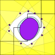
We put the at most $\varhexagon_{P}$ vertices of ${\mathcal{CH}}\left({P\cap C}\right)$ into a query set. Querying these points is enough to label correctly all points inside the body $C$. As for the points of $P$ outside $C$, let $T\subseteq P\setminus C$ be the minimum size subset such that querying these points correctly labels all points outside $C$. Each point $p\in T$ is associated with a halfspace $h^{+}_{p}$ that contains $C$. Let $H$ be this set of halfspaces. Observe that for any point $p\in T$, there is a point $\mathrm{witness}(p)\in P\setminus C$ for which $h^{+}_{p}$ does not contain $\mathrm{witness}(p)$ (as otherwise, $p$ can be removed from $T$). Let $U=\left\{\mathrm{witness}(p)\;\middle|\;p\in T\right\}$. The points of $U$ are in the faces of the arrangement $\mathcal{A}\left({H}\right)$ that are adjacent to the face $\cap_{p\in T}h^{+}_{p}$, see Figure 2.4.

Since each point of $U$ is separable by a line from the remaining points of $U$, it follows that $U$ is convex. As such, $\left|{T}\right|=\left|{U}\right|\leq\varhexagon_{P}$ which implies the result.  

The above lemma implies that the inference dimension of $P$ is $2\varhexagon_{P}$. Plugging this into the algorithm of Kane et al. [KLMZ17] results in an algorithm that labels all points correctly and performs the same number of queries as Theorem 2.8 in expectation. The advantage of Theorem 2.8 is that it does not require knowing the value of $\varhexagon_{P}$ in advance. However, one could perform an exponential search for a tight upper bound on $\varhexagon_{P}$, and still use the algorithm of Kane et al. [KLMZ17]. We leave the question of experimentally comparing the two algorithms as an open problem for future research.

Sketch of the algorithm of [KLMZ17].

The algorithm of Kane et al. [KLMZ17] specialized for our case works as follows. Start by randomly picking a sample of size $O(\varhexagon_{P})$ and query the oracle with each of these points. Next, stream the unlabeled points through the computed regions, leaving only the points that are yet to be labeled. The algorithm repeats this process $O(\log n)$ times, in each iteration working on the remaining unlabeled points. By proving that in expectation at least half of the points are being labeled at each round, it follows that $O(\log n)$ iterations suffice.

2.3 The greedy algorithm in 3D

Consider the 3D variant of the 2D problem: Given a set of points $P$ in $\mathbb{R}^{3}$ and a convex body $C$ specified via a separation oracle, the task at hand is to classify, for all the points of $P$, whether or not they are in $C$, using the fewest oracle queries possible.

The greedy algorithm naturally extends, where at each iteration $i$ a plane $\mathcalb{e}_{i}$ is chosen that is tangent to the current inner approximation $B_{i}$, such that it’s closed halfspace (which avoids the interior of $B_{i}$) contains the largest number of unclassified points from the set $U_{i}$. If the queried centerpoint is outside, the oracle returns a separating plane and as such points can be discarded by the remove operation. Similarly, if the centerpoint is reported inside, then the algorithm calls the expand and updates the 3D inner approximation $B_{i}$.

2.3.1 Analysis

Following the analysis of the greedy algorithm in 2D, we (conceptually) maintain the following set of objects: For a point $p\in U_{i}$, let $\mathcalb{d}_{i}(p)$ be the set of all unit length directions $v\in\mathbb{R}^{3}$ such that a plane perpendicular to $v$ separates $p$ from $B_{i}$. Let $\mathcal{P}_{i}=\left\{\mathcalb{d}_{i}(p)\;\middle|\;p\in U_{i}\right\}$. A set of objects form a collection of pseudo-disks if the boundary of every pair of them intersect at most twice. The following claim shows that $\mathcal{P}_{i}$ is a collection of pseudo-disks on $\mathbb{S}$, where $\mathbb{S}$ is the sphere of radius one centered at the origin.

Lemma 2.11.

The set $\mathcal{P}_{i}=\left\{\mathcalb{d}_{i}(p)\subseteq\mathbb{S}\;\middle|\;p\in U_{i}\right\}$ is a collection of pseudo-disks.

Proof:

Fix two points $p,r\in U_{i}$ such that the boundaries of $\mathcalb{d}_{i}(p)$ and $\mathcalb{d}_{i}(r)$ intersect on $\mathbb{S}$. Let $\mathcalb{l}$ be the line in $\mathbb{R}^{3}$ passing through $p$ and $r$. Consider any plane $\mathcalb{e}$ such that $\mathcalb{l}$ lies on $\mathcalb{e}$. Since $\mathcalb{l}$ is fixed, $\mathcalb{e}$ has one degree of freedom. Conceptually rotate $\mathcalb{e}$ until becomes tangent to $B_{i}$ at point $u^{\prime}$. The direction of the normal to this tangent plane, is a point in $X=\partial\mathcalb{d}_{i}(p)\cap\partial\mathcalb{d}_{i}(r)$. Note that this works also in the other direction — any point in $X$ corresponds to a tangent plane passing through $\mathcalb{l}$. The family of planes passing through $\mathcalb{l}$ has only two tangent planes to $C$. It follows that $\left|{X}\right|=2$. As such, any two regions in $\mathcal{P}_{i}$ intersect as pseudo-disks.  

We need the following two classical results that follows from the Clarkson-Shor [CS89] technique.

Lemma 2.12.

Let $\mathcal{P}$ be a collection of $n$ pseudo-disks, and let $V_{\!\leq k}\left({\mathcal{A}}\right)$ be the set of all vertices of depth at most $k$ in the arrangement $\mathcal{A}=\mathcal{A}\left({\mathcal{P}}\right)$. Then $\left|{V_{\!\leq k}\left({\mathcal{A}}\right)}\right|=O(nk)$.

Proof:

Let $S\subseteq\mathcal{V}$ be a random sample where each pseudo-disk is independently placed into $S$ with probability $1/k$. For each $p\in V_{\!\leq k}\left({\mathcal{A}}\right)$, let $\mathcal{E}_{p}$ be the event that $p$ is a vertex in the union $\mathcal{U}\left({S}\right)$ of this random subset of pseudo-disks. The probability that $p$ is part of the union is at least the probability that both pseudo-disks defining $p$ in $\mathcal{A}$ are sampled into $S$ and the remaining $k-2$ objects containing $p$ are not in $S$. Thus,

$$\mathop{\mathbf{Pr}}\!\left[{\mathcal{E}_{p}}\right]\geq\frac{1}{k^{2}}\left({1-\frac{1}{k}}\right)^{k}\geq\frac{1}{e^{2}k^{2}},$$

since $1-1/x\geq e^{-2/x}$ for $x\geq 2$. If $\left|{\mathcal{U}\left({S}\right)}\right|$ denotes the number of vertices on the boundary of the union, then linearity of expectations imply $\mathop{\mathbf{E}}\!\left[{\left|{\mathcal{U}\left({S}\right)}\right|}\right]\geq\left|{V_{\!\leq k}\left({\mathcal{A}}\right)}\right|/(e^{2}k^{2})$. On the other hand, it is well known the union complexity of a collection of $n$ pseudo-disks is $O(n)$ [KLPS86]. Therefore, $\mathop{\mathbf{E}}\!\left[{\left|{\mathcal{U}\left({S}\right)}\right|}\right]\leq\mathop{\mathbf{E}}\!\left[{c\left|{S}\right|}\right]\leq cn/k$, for some appropriate constant $c$. Putting both bounds on $\mathop{\mathbf{E}}\!\left[{\left|{\mathcal{U}\left({S}\right)}\right|}\right]$ together, it follows that $cn/k\geq\left|{V_{\!\leq k}\left({\mathcal{A}}\right)}\right|/(e^{2}k^{2})\iff\left|{V_{\!\leq k}\left({\mathcal{A}}\right)}\right|=O(nk)$.  

Lemma 2.13.

Let $\mathcal{P}$ be a collection of $n$ pseudo-disks. For two integers $0<t\leq k$, a subset $X\subseteq\mathcal{P}$ is a $(t,k)$-tuple if (i) $\left|{X}\right|\leq t$, (ii) $\exists p\in\cap_{\mathcalb{d}\in X}\mathcalb{d}$, and (iii) $\mathrm{depth\left({p,\mathcal{P}}\right)}\leq k$. Let $L\left({t,k,n}\right)$ be the set of all $(\leq t,k)$-tuples of $\mathcal{P}$. Then $\left|{L\left({t,k,n}\right)}\right|=O(ntk^{t-1})$.

Proof:

Let $R\subseteq\mathcal{P}$ be a random sample, where each pseudo-disk is independently placed into $R$ with probability $1/k$. Consider a specific $(t,k)$-tuple $X$, with a witness point $p$ of depth $\leq k$. Without loss of generality, by moving $p$, one can assume $p$ is a vertex of $\mathcal{A}\left({\mathcal{P}}\right)$.

Let $\mathcal{E}_{X}$ be the event that $p$ is of depth exactly $t$ in $\mathcal{A}\left({R}\right)$, and $X\subseteq R$. For $\mathcal{E}_{X}$ to occur, all the objects of $X$ need to be sampled into $R$, and each of the at most $k-t$ pseudo-disks containing $p$ in its interior are not in $R$. Therefore

$$\mathop{\mathbf{Pr}}\!\left[{\mathcal{E}_{X}}\right]\geq\frac{\left({1-1/k}\right)^{\mathrm{depth\left({p,\mathcal{P}}\right)}-|X|}}{k^{|X|}}\geq\frac{\left({1-1/k}\right)^{k}}{k^{t}}\geq\frac{1}{e^{2}k^{t}}.$$

Note, that a vertex of depth $\leq k$ in $\mathcal{A}\left({R}\right)$ corresponds to at most one such an event happening. We thus have, by linearity of expectations, that

$$\frac{\left|{L\left({t,k,n}\right)}\right|}{e^{2}k^{t}}\leq\mathop{\mathbf{E}}\!\left[{\bigl{.}\left|{V_{\!\leq t}\left({\mathcal{A}\left({R}\right)}\right)}\right|}\right]=O(tn/k),$$

by Lemma 2.12.  

Lemma 2.14.

Let $G_{i}=(\mathcal{P}_{i},E_{i})$ be the intersection graph of the pseudo-disks of $\mathcal{P}_{i}$ (in the $i$th iteration). If $\mathcal{A}\left({\mathcal{P}_{i}}\right)$ has maximum depth $k$, then $\left|{E_{i}}\right|=O(nk)$. Furthermore, $\alpha(G_{i})=\Omega(n/k)$, where $\alpha(G_{i})$ denotes the size of the largest independent set in $G_{i}$.

Proof:

The first claim follows from Lemma 2.13. Indeed, $\left|{E_{i}}\right|=L\left({2,k,n}\right)=O(nk)$ — since every intersecting pair of pseudo-disks induces a corresponding $(2,k)$-tuple.

For the second part, Turán’s Theorem states that any graph has an independent set of size at least $n/\left({{d}_{\mathrm{avg}}(G_{i})+1}\right)$, where ${d}_{\mathrm{avg}}(G_{i})=2\left|{E_{i}}\right|/n\leq ck$ is the average degree of $G_{i}$ and $c$ is some constant. It follows that $\alpha(G_{i})\geq n/(ck+1)=\Omega(n/k)$.  

The challenge in analyzing the greedy algorithm in 3D is that mutual visibility between pairs of points is not necessarily lost as the inner approximation grows. As an alternative, consider the hypergraph $H_{i}=(\mathcal{P}_{i},\mathcal{E}_{i})$, where a triple of pseudo-disks $\mathcalb{d}_{1},\mathcalb{d}_{2},\mathcalb{d}_{3}\in\mathcal{P}_{i}$ form a hyperedge $\left\{{\mathcalb{d}_{1},\mathcalb{d}_{2},\mathcalb{d}_{3}}\right\}\in\mathcal{E}_{i}$ $\iff$ $\mathcalb{d}_{1}\cap\mathcalb{d}_{2}\cap\mathcalb{d}_{3}\neq\varnothing$ (this is equivalent to the condition that the corresponding triple of points span a triangle which does not intersect $B_{i}$).

As in the analysis of the algorithm in 2D, we first bound the number of edges in $H_{i}$ and then argue that enough progress is made in each iteration.

Lemma 2.15.

Let $H_{i}=(\mathcal{P}_{i},\mathcal{E}_{i})$ be the hypergraph in iteration $i$, and let $G_{i}$ be the corresponding intersection graph of $\mathcal{P}_{i}$. If $\mathcal{A}\left({\mathcal{P}_{i}}\right)$ has maximum depth $k$, then $\left|{\mathcal{E}_{i}}\right|=O(\alpha(G_{i})k^{3})$.

Proof:

Lemma 2.14 implies that $G_{i}$ has an independent set of size $\Omega(f_{i}/k)$, where $f_{i}=\left|{\mathcal{P}_{i}}\right|$. Lemma 2.13 implies that $\left|{\mathcal{E}_{i}}\right|\leq\left|{L\left({3,k,f_{i}}\right)}\right|=O(f_{i}k^{2})=O(\alpha(G_{i})k^{3})$.  

The following is a consequence of the Colorful Carathéodory Theorem [Bár82], see Theorem 9.1.1 in [Mat02].

Theorem 2.16.

Let $P$ be a set of $n$ points in $\mathbb{R}^{d}$ and $\mathcalb{c}$ be the centerpoint of $P$. Let $S=\binom{P}{d+1}$ be the set of all $d+1$ simplices induced by $P$. Then for sufficiently large $n$, the number of simplices in $S$ that contain $\mathcalb{c}$ in their interior is at least $c_{d}n^{d+1}$, where $c_{d}$ is a constant depending only on $d$.

Next, we argue that in each iteration of the greedy algorithm, a constant fraction of the edges in $H_{i}$ are removed. The following is the higher dimensional version of Lemma 2.5.

Lemma 2.17.

Let $P$ be a set of $n$ points in $\mathbb{R}^{3}$ lying above the $xy$-plane, $\mathcalb{c}$ be the centerpoint of $P$ and $T=\binom{P}{3}$ be the set of all triangles induced by $P$. Next, consider any point $r$ on the $xy$-plane. Then the segment $\mathcalb{c}r$ intersects at least $\Omega(n^{3})$ triangles of $T$.

Proof:

Let $S=\binom{P}{d+1}$ be the set of all simplices induced by $P$. Theorem 2.16 implies that the centerpoint $\mathcalb{c}$ is contained in $n^{4}/c_{1}$ simplices of $S$ for some constant $c_{1}>1$. Let $K$ be a simplex that contains $\mathcalb{c}$ and observe the segment $\mathcalb{c}r$ must intersect at least one of the triangular faces $\tau$ of $K$. As $K\in S$, charge this simplex $K$ to the triangular face $\tau$. Applying this counting to all the simplices containing $\mathcalb{c}$, implies that at least $n^{4}/c_{1}$ charges are made. On the other hand, a triangle $\tau$ can be charged at most $n-3$ times (because a simplex can be formed from $\tau$ and one other additional point of $P$). It follows that $\mathcalb{c}r$ intersects at least $(n^{4}/c_{1})/(n-3)=\Omega(n^{3})$ triangles of $T$.  

Lemma 2.18.

In each iteration of the greedy algorithm, the number of edges in the hypergraph $H_{i}=(\mathcal{P}_{i},\mathcal{E}_{i})$ decreases by at least $\Omega(k^{3})$, where $k$ is the maximum depth of any point in $\mathcal{A}\left({\mathcal{P}_{i}}\right)$.

Proof:

Recall that $U^{+}=U_{i}\cap\mathcalb{e}^{+}$ is the current set of unclassified points and $\mathcalb{e}$ is the plane tangent to $B_{i}$, where $\mathcalb{e}^{+}$ is the closed halfspace that avoids the interior of $B_{i}$ and contains the largest number of unlabeled points. Note that $|U^{+}|\geq k$.

In a remove operation, arguing as in Lemma 2.6, implies that the number of points of $U^{+}$ that are discarded is at least $t_{i}\geq k/4$. Since all of the discarded points are in a halfspace avoiding $B_{i}$, it follows that all the triples they induce are in $H_{i}$. Namely, at least $\binom{t_{i}}{3}=\Omega(k^{3})$ hyperedges get discarded.

In an expand operation, the centerpoint $\mathcalb{c}$ of $U^{+}$ is added to the current inner approximation $B_{i}$. Since all of the points of $U^{+}$ lie above the plane $\mathcalb{e}$, applying Lemma 2.17 on $U^{+}$ with the centerpoint $\mathcalb{c}$ and a point lying on the plane $\mathcalb{e}$ inside the (updated) inner approximation, we deduce that at least $\Omega(k^{3})$ hyperedges are removed.  

Theorem 2.19.

Let $C\subseteq\mathbb{R}^{3}$ be a convex body provided via a separation oracle, and let $P$ be a set of $n$ points in $\mathbb{R}^{3}$. The greedy classification algorithm performs ${O\bigl{(}(\varhexagon_{P}+1)\log n\bigr{)}}$ oracle queries. The algorithm correctly identifies all points in $P\cap C$ and $P\setminus C$.

Proof:

The proof is essentially the same as Theorem 2.8. Arguing as in Lemma 2.1 implies that there are at most $O(\log n)$ iterations (and thus also oracle queries) in which the inner approximation is empty.

Now consider the hypergraph $H_{1}=(\mathcal{P}_{1},\mathcal{E}_{1})$ at the start of the algorithm execution. As the algorithm progresses, both vertices and hyperedges are removed from the hypergraph. Let $H_{i}=(\mathcal{P}_{i},\mathcal{E}_{i})$ denote the hypergraph in the $i$th iteration of the algorithm. Recall that $\mathcal{P}_{i}$ is a set of pseudo-disks associated with each of the points yet to be classified. Observe that any independent set of pseudo-disks in the corresponding intersection graph $G_{i}$ corresponds to an independent set of points with respect to the inner approximation $B_{i}$, and as such is a subset of points in convex position. Therefore, the size of any such independent set is bounded by $\varhexagon_{P}$.

Let $k_{i}$ denote the maximum depth of any vertex in the arrangement $\mathcal{A}\left({\mathcal{P}_{i}}\right)$. Lemma 2.15 implies that $\left|{\mathcal{E}_{i}}\right|=O\left({\varhexagon_{P}k_{i}^{3}}\right)$. Lemma 2.18 implies that the number of hyperedges in the $i$th iteration decreases by at least $\Omega(k_{i}^{3})$. Namely, after $O(\varhexagon_{P})$ iterations, the maximum depth is halved. It follows that after $O(\varhexagon_{P}\log n)$ iterations, the maximum depth is zero, which implies that all the points are classified. Since the algorithm performs one query per iteration, the claim follows.  

3 An instance-optimal approximation in two dimensions

Before discussing the improved algorithm, we present a lower bound on the number of oracle queries performed by any algorithm that classifies all the given points. We then present the improved algorithm, which matches the lower bound up to a factor of $O(\log^{2}n)$.

3.1 A lower bound

Given a set $P$ of points in the plane, and a convex body $C$, the outer fence of $P$ is a closed convex polygon $F_{\mathrm{out}}$ with minimum number of vertices, such that $C\subseteq F_{\mathrm{out}}$ and $C\cap P=F_{\mathrm{out}}\cap P$. Similarly, the inner fence is a closed convex polygon $F_{\mathrm{in}}$ with minimum number of vertices, such that $F_{\mathrm{in}}\subseteq C$ and $C\cap P=F_{\mathrm{in}}\cap P$. Intuitively, the outer fence separates $P\setminus C$ from $\partial C$, while the inner fence separates $P\cap C$ from $\partial C$. The separation price of $P$ and $C$ is

$$\varocircle\left({P,C}\right)=\left|{F_{\mathrm{in}}}\right|+\left|{F_{\mathrm{out}}}\right|,$$

where $\left|{F}\right|$ denotes the number of vertices of a polygon $F$. See Figure 3.1 for an example.

Figure 3.1: The separation price, for the same point set, is different depending on how “tight” the body is in relation to the inner and outer point set.

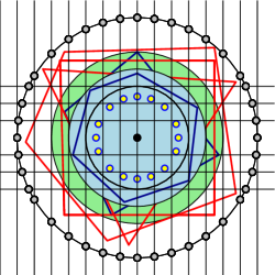
Lemma 3.1.

Let $C$ be a convex body provided via a separation oracle, and let $P$ be a point set in the plane. Any algorithm that classifies the points of $P$ in relation to $C$, must perform at least $\varocircle\left({P,C}\right)$ separation oracle queries.

Proof:

Consider the set $Q$ of queries performed by the optimal algorithm (for this input), and split it, into the points inside and outside $C$. The set of points inside, $Q_{\mathrm{in}}=Q\cap C$ has the property that $Q_{\mathrm{in}}\subseteq C$, and furthermore ${\mathcal{CH}}\left({Q_{\mathrm{in}}}\right)\cap P=C\cap P$ — otherwise, there would be a point of $C\cap P$ that is not classified. Namely, the vertices of ${\mathcal{CH}}\left({Q_{\mathrm{in}}}\right)$ are vertices of a fence that separates the points of $P$ inside $C$ from the boundary of $C$. As such, we have that $\left|{Q_{\mathrm{in}}}\right|\geq\left|{{\mathcal{CH}}\left({Q_{\mathrm{in}}}\right)}\right|\geq\left|{F_{\mathrm{in}}}\right|$.

Similarly, each query in $Q_{\mathrm{out}}=Q\setminus Q_{\mathrm{in}}$ gives rise to a separating halfplane. The intersection of the corresponding halfplanes is a convex polygon $H$ that contains $C$, and furthermore contains no point of $P\setminus C$. Namely, the boundary of $H$ behaves like an outer fence. As such, we have $\left|{Q_{\mathrm{out}}}\right|\geq\left|{H}\right|\geq\left|{F_{\mathrm{out}}}\right|$.

Combining, we have that $\left|{Q}\right|=\left|{Q_{\mathrm{in}}}\right|+\left|{Q_{\mathrm{out}}}\right|\geq\left|{F_{\mathrm{in}}}\right|+\left|{F_{\mathrm{out}}}\right|=\varocircle\left({P,C}\right)$, as claimed.  

Remarks.

1. Naturally the separation price, and thus the proof of the lower bound, generalizes to higher dimensions. See Definition A.1 and Lemma A.2.

2. The lower bound only holds for $d\geq 2$. In 1D, the problem can be solved using $O(\log n)$ queries with binary search. The above would predict that any algorithm needs $\Omega(1)$ queries. However it is not hard to argue a stronger lower bound of $\Omega(\log n)$.

3. In Appendix A, we show that when $P$ is a set of $n$ points chosen uniformly at random from a square and $C$ is a smooth convex body, $\mathop{\mathbf{E}}\!\left[{\varocircle\left({P,C}\right)}\right]=O(n^{1/3})$. Thus, when the points are randomly chosen, one can think of $\varocircle\left({P,C}\right)$ as growing sublinearly in $n$.

3.2 Useful operations

We start by presenting some basic operations that the new algorithm will use.

3.2.1 A directional climb

Given a direction $v$, a directional climb is a sequence of iterations, where in each iteration, the algorithm finds the extreme line $\ell$ perpendicular to $v$, that is tangent to the inner approximation $B$. The algorithm then performs an iteration with $\ell$, as described in Section 2.2.2, which we now recall. Specifically, the algorithm computes the centerpoint $q$ of all points in the halfspace bounded by $\ell$ that avoids $C$. Depending on whether $q\in C$, we either perform ${{\color[rgb]{0.59,0,0.66}\texttt{\bf{expand}}}}{}(q)$ or ${{\color[rgb]{0.59,0,0.66}\texttt{\bf{remove}}}}{}(\ell)$ (see Section 2.2.1). We then classify points accordingly and recompute $\ell$ with the updated inner approximation $B$. See Figure 3.2 for an illustration. The directional climb ends when the outer halfspace induced by this line contains no unclassified point.

Figure 3.2: A directional climb. An iteration is done using the line $\mathcalb{l}$. After updating $B$ to include the query $q$, the algorithm chooses a new extreme line $\mathcalb{h}$ tangent to $B$ in the direction of $v$.

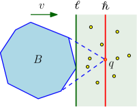
Lemma 3.2.

A directional climb requires $O(\log n)$ oracle queries.

Proof:

Consider the tangent to $B$ in the direction of $v$. At each iteration, we claim the number of points in this halfplane is reduced by a factor of $1/3$. Indeed, if the query (i.e., centerpoint) is outside $C$ then at least a third of these points got classified as being outside. Alternatively, the tangent halfplanes moves in the direction of $v$, since the query point is inside $C$. But then the new halfspace contains at most $2/3$ fraction of the previous point set — again, by the centerpoint property.  

3.2.2 Line cleaning

Figure 3.3: Unclassified points and their pockets.

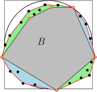
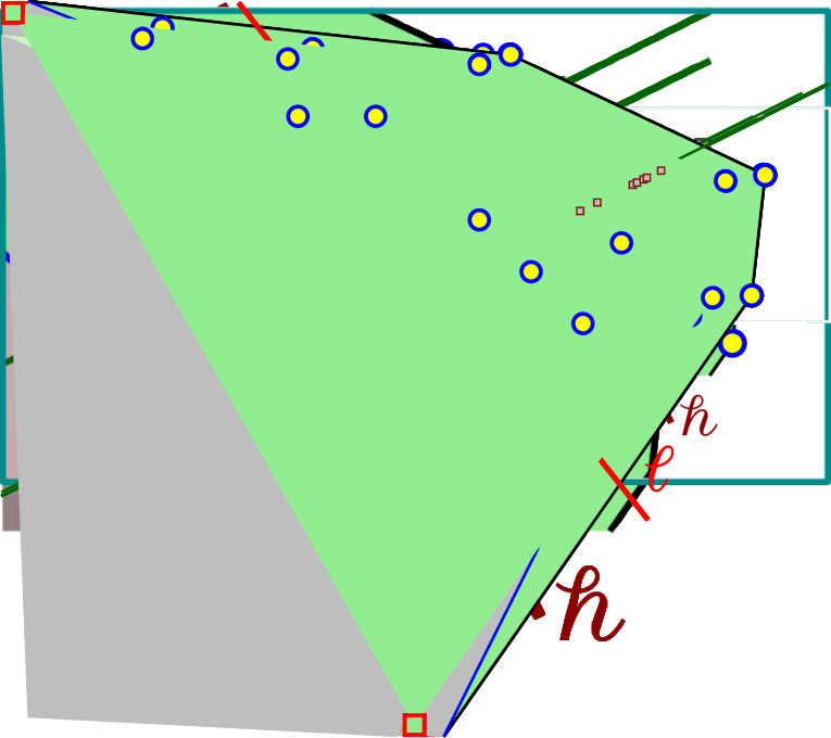
A pocket is a connected region of ${\mathcal{CH}}\left({U\cup B}\right)\setminus B$, see Figure 3.3. For the set $P$ of input points, consider the set of all lines

$$L\left({P}\right)=\left\{\mathrm{line}(p,r)\;\middle|\;p,r\in P\right\}$$ (3.1)

they span.

Let $\mathcalb{l}$ be a line that splits a pocket $\Upsilon$ into two regions, and furthermore, it intersects $B$. Let $I=\mathcalb{l}\cap\Upsilon$, and consider all the intersection points of interest along $I$ in this pocket. That is,

$$\Xi\left({\Upsilon,\mathcalb{l},P}\right)=I\cap L\left({P}\right)=\left\{\bigl{.}(\Upsilon\cap\mathcalb{l})\cap\mathcalb{h}\;\middle|\;\mathcalb{h}\in L\left({P}\right)\right\}.$$

In words, we take all the pairs of points of $P$ (each such pair induces a line) and we compute the intersection points of these lines with the interval $I$ of interest. Ordering the points of this set along $\mathcalb{l}$, a prefix of them is in $C$, while the corresponding suffix are all outside $C$. One can easily compute this prefix/suffix by doing a binary search, using the separation oracle for $C$ — see the lemma below for details. Each answer received from the oracle is used to update the point set, using expand or remove operations, as described in Section 2.2.1. We refer to this operation along $\mathcalb{l}$ as cleaning the line $\mathcalb{l}$. See Figure 3.4.

Figure 3.4: Line cleaning. All the intersection points of interest along $\mathcalb{l}$ are classified. The binary search results in the oracle returning a line $\mathcalb{h}$ that separates the points outside from the points inside.

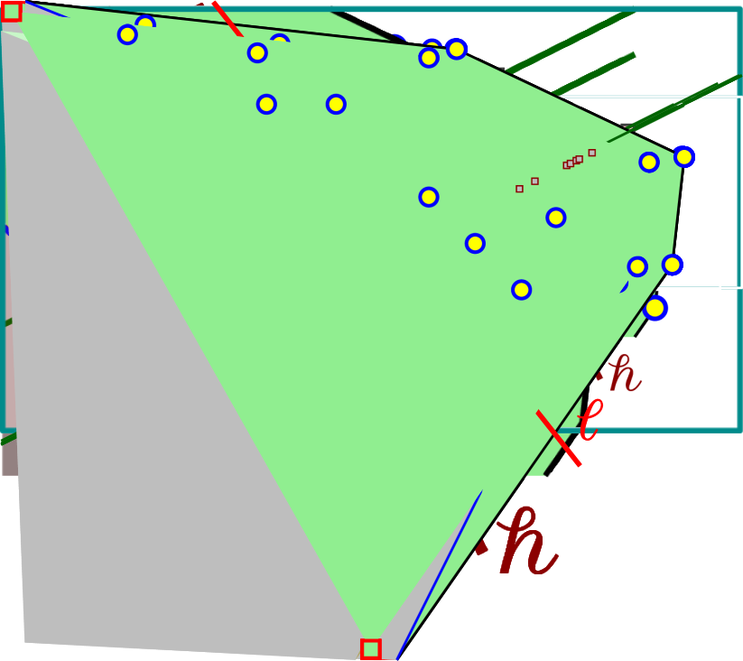
Lemma 3.3.

Given a pocket $\Upsilon$, and a splitting line $\mathcalb{l}$, one can clean the line $\mathcalb{l}$ — that is, classify all the points of $\Xi=\Xi\left({\Upsilon,\mathcalb{l},P}\right)$ using $O\left({\log n\bigr{.}}\right)$ oracle queries. By the end of this process, $\Upsilon$ is replaced by two pockets, $\Upsilon_{1}$ and $\Upsilon_{2}$ that do not intersect $\mathcalb{l}$. The pockets $\Upsilon_{1}$ or $\Upsilon_{2}$ may be empty sets.

Proof:

First, we describe the line cleaning procedure in more detail. The algorithm maintains, in the beginning of the $i$th iteration, an interval $J_{i}$ on the line $\mathcalb{l}$ containing all the points of $\Xi$ that are not classified yet. Initially, $J_{1}=\Upsilon\cap\mathcalb{l}$. One endpoint, say $p_{i}\in J_{i}$ is on $\partial B_{i}$, and the other, say $p_{i}^{\prime}$, is outside $C$, where $B_{i}$ is the inner approximation in the beginning of the $i$th iteration.

In the $i$th iteration, the algorithm computes the set $\Xi_{i}=J_{i}\cap\Xi$. If this set is empty, then the algorithm is done. Otherwise, it picks the median point $u_{i}$, in the order along $\mathcalb{l}$ in $\Xi_{i}$, and queries the oracle with $u_{i}$. There are two possibilities:

1. If $u_{i}\in C$ then the algorithm sets $\Xi_{i+1}=\Xi_{i}\setminus[p_{i},u_{i})$, and $J_{i+1}=J_{i}\setminus[p_{i},u_{i})$.

2. If $u_{i}\notin C$, then the oracle provided a closed halfspace $h^{+}$ that contains $C$. Let $h^{-}$ be the complement open halfspace that contains $u_{i}$. The algorithm sets $\Xi_{i+1}=\Xi_{i}\setminus h^{-}$ and $J_{i+1}=J_{i}\cap h^{+}$.

This resolves the status of at least half the points in $\Xi_{i}$, and shrinks the active interval. The algorithm repeats this till $\Xi_{i}$ becomes empty. Since $\left|{\Xi}\right|=O(n^{2})$, this readily implies that the algorithm performs $O(\log n)$ iterations.

We now argue that the pocket is split — that is, $\Upsilon_{1}$ and $\Upsilon_{2}$ do not intersect $\mathcalb{l}$. Assume that it is false, and let $B^{\prime}$ be the inner approximation after this procedure is done. Let $L$ (resp. $R$) be the points of $U_{\Upsilon}=U\cap\Upsilon$ that are unclassified on one side (resp. other side) of $\mathcalb{l}$. If the pocket is not split, then there are two points $p\in L$ and $r\in R$, such that $pr\cap B^{\prime}=\emptyset$, and $\partial{\mathcal{CH}}\left({B^{\prime}\cup L\cup R}\right)$ intersects $\mathcalb{l}$ at the point $u=pr\cap\mathcalb{l}$. However, by construction, the point $u\in\Xi$. As such, the point $u$ is now classified as either being inside or outside $C$, as it is a point in $\Xi$. If $u$ is outside, then the halfplane $h^{-}$ that classified it as such, must had classified either $p$ or $r$ as being outside $C$, which is a contradiction. The other option, is that $u$ is classified as being inside, but then, it is in $B^{\prime}$, which is again a contradiction, as it implies that $B^{\prime}$ intersects the segment $pr$.  

3.2.3 Vertical pocket splitting

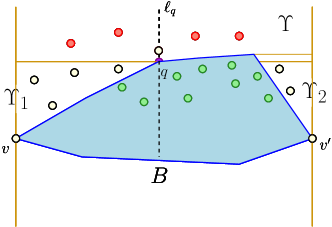
Consider a pocket $\Upsilon$ such that all of its points lie vertically above $B$, and the bottom of $\Upsilon$ is part of a segment of $\partial B$, see Figure 3.5. Such a pocket can be viewed as being defined by an interval on the $x$-axis corresponding to its two vertical walls. Let $U_{\Upsilon}$ be the set of unclassified points in this pocket. In each iteration, the algorithm computes the centerpoint $q$ of $U_{\Upsilon}$, and queries the separation oracle for the label of $q$. As long as the query point is outside $C$, the algorithm performs a remove operation using the returned separating line.

When the oracle returns that the query point $q$ is inside $C$, the algorithm computes the vertical line $\mathcalb{l}_{q}$ through $q$. The algorithm now performs line cleaning on this vertical line. This operation splits $\Upsilon$ into two sub-pockets. Crucially, since $q$ was a centerpoint for $U_{\Upsilon}$, the number of points in each of the two sub-pockets is at most $2\left|{U_{\Upsilon}}\right|/3$. See Figure 3.5.

Figure 3.5: Vertical pocket splitting. In this example, the centerpoint $q$ lies inside $C$. Thus we construct the vertical line $\ell_{q}$ through $q$ (left). Next, we perform a line cleaning operation on $\ell_{q}$. This splits the original pocket $\Upsilon$ into two new pockets $\Upsilon_{1}$, $\Upsilon_{2}$, while classifying some points in the process (right). Observe that the unclassified points in $\Upsilon_{1}$ and $\Upsilon_{2}$ are no longer mutually visible to each other after the line cleaning operation.

3.3 The algorithm

The algorithm starts in the same way as the greedy algorithm of Section 2.2.2, which we restate for convenience. Recall that $U$ is the set of unclassified points (initially $U=P$). At all times, the algorithm maintains the inner approximation $B\subseteq C$. At the beginning, $B$ is uninitialized. The algorithm computes the centerpoint $q$ of $U$ and queries the oracle for the label of $q$. While $q$ is outside, we classify the appropriate set of points as outside (according to the separating hyperplane returned from the oracle), update $U$, and repeat. As soon as the computed centerpoint $q$ lies in $C$, we set $B=q$ and continue to the next stage.

Next, the algorithm performs two directional climbs (Section 3.2.1) in the positive and negative directions of the $x$-axis. This uses $O(\log n)$ oracle queries by Lemma 3.2 and results in a computed segment $vv^{\prime}\subseteq C$, where $v,v^{\prime}$ are vertices of the inner approximation $B$, such that all unclassified points lie in the strip induced by the vertical line through $v$ and the vertical line through $v^{\prime}$, see also Figure 3.5.

The algorithm now handles all points of $U$ lying above $vv^{\prime}$ (the points below the line are handled in a similar fashion). Let $B^{+}$ be the set of vertices of $B$ in the top chain. Note that $B^{+}$ consists of at most $O(\log n)$ vertices. For each vertex $v$ of $B^{+}$, the algorithm performs line cleaning on the vertical line going through $v$. This results in $O(\log n)$ vertical pockets, where all vertical lines passing originally through $B^{+}$ are now clean.

The algorithm repeatedly picks a vertical pocket. If the pocket contains less than three points the algorithm queries the oracle for the classification of these points, and continues to the next pocket. Otherwise, the algorithm performs a vertical pocket splitting operation, as described in Section 3.2.3. The algorithm stops when there are no longer any pockets (i.e., all the points above the segment $vv^{\prime}$ are classified). The algorithm then runs the symmetric procedure below this segment $vv^{\prime}$.

3.4 Analysis

Figure 3.6: Constructing the polygon $\pi$ from an inner fence $\sigma$.

Lemma 3.4.

Given a point set $P$, and a convex polygon $\sigma$ that is an inner fence for $P\cap C$; that is, $P\cap C\subseteq\sigma\subseteq C$. Then, there is a convex polygon $\pi$, such that

1. $P\cap C\subseteq\pi\subseteq\sigma$.

2. $\left|{\pi}\right|\leq 2\left|{\sigma}\right|$ (where $\left|{Q}\right|$ denotes the number of vertices of the polygon $Q$).

3. Every edge of $\pi$ lies on a line of $L\left({P}\right)$, see Eq. (3.1).

Proof:

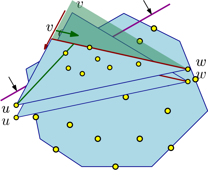
Any edge $e$ of $\sigma$ that does not contain any point of $P$ on it can be moved parallel to itself into the polygon until it passes through a point of $P$. Next, split the edges that contain only a single point of $P$, by adding this point as a vertex.

Consider a vertex $v$ of the polygon that is not in $P$ — and consider the two adjacent vertices $u,w$, which must be in $P$. If $\triangle uvw\setminus uw$ contains no point of $P$, then we delete $v$ from the polygon and replace it by the edge $uw$. Otherwise, move $v$ towards $u$, until the edge $vw$ hits a point of $P$. Next, move $v$ towards $w$, till the edge $vu$ hits a point of $P$. See Figure 3.6.

Repeating this process so that all edges contain two points of $P$ means that properties (A) and (C) are met. Additionally, the number of edges of the new polygon $\pi$ is at most twice the number of edges of $\sigma$, implying property (B).  

Consider the inner and outer fences $F_{\mathrm{in}}$ and $F_{\mathrm{out}}$ of $P$ in relation to $C$. Applying Lemma 3.4 to $F_{\mathrm{in}}$, results in a convex polygon $\pi$ that separates $P\cap C$ from $\partial C$, that has at most $2\left|{F_{\mathrm{in}}}\right|$ vertices. Let ${V}$ be the set of all vertices of the polygons $F_{\mathrm{in}},F_{\mathrm{out}}$ and $\pi$.

The following two Lemmas state that if a vertical pocket $\Upsilon$ containing no vertex of ${V}$, then all points in $\Upsilon$ can be classified using $O(\log n)$ oracle queries. Finally, we analyze the scenario when $\Upsilon$ contains at least one vertex of ${V}$.

Lemma 3.5.

Let $\Upsilon$ be a vertical pocket created during the algorithm with current inner approximation $B$. Suppose that ${V}\cap\Upsilon=\varnothing$, then all points in $P\cap\Upsilon$ are outside $C$.

Proof:

Assume without loss of generality that $\Upsilon$ lies above $B$. Let $U=P\cap\Upsilon$ be the set of unclassified points in the pocket. Note that $\Upsilon$ is bounded by two vertical lines that were previously cleaned.

By assumption, $\Upsilon$ does not contain any vertex of $\pi$. It follows that there is a single edge of $\pi$ that intersects the two vertical lines bounding $\Upsilon$. Let $u_{L},u_{R}$ be these two intersection points, one lying on each line. By definition, we have $u_{L},u_{R}\in C$. Furthermore, $u_{L},u_{R}$ lie on lines of $L\left({P}\right)$ by construction of $\pi$. Since both vertical lines bounding $\Upsilon$ were cleaned, it must be that the segment $u_{L}u_{R}\subseteq B$. Since all points of $U$ are above $B$, this implies that $U$ lies above $u_{L}u_{R}$ and thus above $\pi$. Namely, all points of $U$ are outside $C$.  

Lemma 3.6.

Let $\Upsilon$ be a vertical pocket with ${V}\cap\Upsilon=\varnothing$. Then during the vertical pocket splitting operation of Section 3.2.3 applied to $\Upsilon$, all oracle queries are outside $C$. In particular, all points of $P\cap\Upsilon$ are classified after $O(\log n)$ oracle queries.

Proof:

Let $U=P\cap\Upsilon$. By Lemma 3.5, all points of $U$ lie outside $C$. Assume that the first statement of the Lemma is false, and let $U^{\prime}\subseteq U$ be the set of unclassified points such that $q$ was the centerpoint for $U^{\prime}$ and $q\in C$. Now $q$ is inside a triangle induced by three points of $U^{\prime}$. Namely, there are (at least) two points outside $C$ in this pocket that are not mutually visible to each other with respect to $C$. But this implies that $F_{\mathrm{out}}$ must have a vertex somewhere inside the vertical pocket $\Upsilon$, which is a contradiction.

Hence, all oracle queries made by the algorithm are outside $C$. Each such query results in a constant reduction in the size of $U$, since the query point is a centerpoint of the unclassified points. It follows that after $O(\log\left|{U}\right|)=O(\log n)$ queries, all points in $\Upsilon$ are classified.  

Theorem 3.7.

Let $C$ be a convex body provided via a separation oracle, and let $P$ be a set of $n$ points in the plane. The improved classification algorithm performs $O\left({\bigl{[}1+\varocircle\left({P,C}\right)\bigr{]}\log^{2}n}\right)$ oracle queries. The algorithm correctly identifies all points in $P\cap C$ and $P\setminus C$.

Proof:

The initial stage involves two directional climbs and $O(\log n)$ line cleaning operations, and thus requires $O(\log^{2}n)$ queries.

A vertical pocket that contains a vertex of ${V}$ is charged arbitrarily to any such vertex. Since the number of points in a pocket reduces by at least a factor of $1/3$ during a split operation, this means that a vertex of ${V}$ is charged at most $O(\log n)$ times. Each time a vertex gets charged, it has to pay for the $O(\log n)$ oracle queries that were issued in the process of creating this pocket, and later on for the price of splitting it. Thus, we only have to account for queries performed in vertical pockets that do not contain a vertex of ${V}$. By Lemma 3.6, such a pocket will have all points inside it classified after $O(\log n)$ oracle queries.

However, the above implies that there are at most $O([1+\varocircle\left({P,C}\right)]\log n)$ vertical pockets with no vertex of ${V}$ throughout the algorithm execution. Since handling such a pocket requires $O(\log n)$ queries, the bound follows.  

4 On emptiness variants in two dimensions

Here, we present two instance-optimal approximation algorithms for solving the following two variants:

1. Emptiness: Find a point $p\in P\cap C$, or using as few queries as possible, verify that $P\cap C=\varnothing$.

2. Reverse emptiness: Find a point $p\in P\setminus(P\cap C)$, or using as few queries as possible, verify that $P\cap C=P$.

For both variants we present $O(\log n)$ approximation (the algorithm for emptiness is randomized), improving over the general approximation algorithm of Section 3 which provides a $O(\log^{2}n)$ approximation.

4.1 Emptiness: Are all the points outside?

Here we consider the problem of verifying that all the given points are outside the convex body.

Algorithm.

The algorithm is a slight modification of the algorithm of Section 2.2.2. Recall the two operations expand and remove that the algorithm will need (Section 2.2.1).

Initially, let $U=P$ be the set of unclassified points. At every round, if the inner approximation $B$ is empty, then the algorithm sets $U^{+}=U$. Otherwise, the algorithm picks a line $\mathcalb{l}$ that is tangent to $B$ with the largest number of points of $U$ on the other side of $\mathcalb{l}$ than $B$. Let $\mathcalb{l}^{-}$ and $\mathcalb{l}^{+}$ be the two closed halfspace bounded by $\mathcalb{l}$, where $B\subseteq\mathcalb{l}^{-}$. The algorithm computes the point set $U^{+}=U\cap\mathcalb{l}^{+}$. We have two cases:

1. Suppose $\left|{U^{+}}\right|$ is of constant size. The algorithm queries the oracle for the status of each of these points. If there exists a point $p\in U^{+}$ which lies in $C$, then we return $p$ as the witness. Otherwise, for each $p\in U^{+}$ we receive a separating line $\mathcalb{l}_{p}$ from the oracle, and the algorithm executes ${{\color[rgb]{0.59,0,0.66}\texttt{\bf{remove}}}}{}(\mathcalb{l}_{p})$.

2. Otherwise, $\left|{U+}\right|$ does not have constant size. The algorithm chooses a point $q\in U^{+}$ at random and queries the oracle using $q$. If $q\in C$, we return $q$ as the witness. Otherwise, we perform a remove operation on the separating line returned.

   Next, we compute the centerpoint $q$ of $U^{+}$ and query the oracle for the label of $q$. Depending on the label of $q$, the algorithm either executes ${{\color[rgb]{0.59,0,0.66}\texttt{\bf{expand}}}}{}(q)$ or ${{\color[rgb]{0.59,0,0.66}\texttt{\bf{remove}}}}{}(\ell)$, where $\ell$ is the separating line in the instance that $q\not\in C$.

Analysis.

Let $G_{i}$ be the intersection graph (see Definition 2.2) over the points outside $C$ in the beginning of the $i$th iteration. We need the following technical Lemma.

Lemma 4.1.

Suppose $P\cap C=\varnothing$. Then at any iteration $i$, the largest independent set in the visibility graph $G_{i}$ is at most $\left|{F_{\mathrm{out}}}\right|$.

Proof:

For the body $C$ and point set $P$, define the set $R\subseteq P$ to be the maximum set of points such that no two points in $R$ are visible with respect to $C$. Observe that $R$ corresponds to the maximum independent set in the visibility graph for $P$ with respect to the body $C$. We claim $\left|{R}\right|\leq\left|{F_{\mathrm{out}}}\right|$. Suppose that $\left|{R}\right|>\left|{F_{\mathrm{out}}}\right|$. Given the polygon $F_{\mathrm{out}}$, for each edge $e$ of $F_{\mathrm{out}}$ consider the line $\mathcalb{l}_{e}$ through $e$ and let $\mathcalb{h}_{e}^{+}$ be the halfspace bounded by $\mathcalb{l}_{e}$ that does not contain $C$ in its interior. Then $\left\{\mathcalb{h}_{e}^{+}\;\middle|\;e\in F_{\mathrm{out}}\right\}$ covers the space $\mathbb{R}^{2}\setminus\mathrm{int}\left({C}\right)$. By the hypothesis, one halfspace $\mathcalb{h}_{e}^{+}$ must contain at least two points of $R$. But then these two such points are visible with respect to $C$, contradicting the definition of $R$.

We know that the size of the largest independent set (with respect to the current inner approximation $B_{i}$) is monotone increasing over the iterations. Hence each independent set can be of size at most $\left|{R}\right|\leq\left|{F_{\mathrm{out}}}\right|$.  

Lemma 4.2.

Let $C$ be a convex body provided via a separation oracle, and let $P$ be a set of $n$ points in the plane. The randomized greedy classification algorithm for emptiness performs ${O\bigl{(}(\left|{F_{\mathrm{out}}}\right|+1)\log n\bigr{)}}$ oracle queries with high probability. The algorithm always correctly verifies that $P\cap C=\varnothing$ or finds a witness point of $P$ inside $C$.

Proof:

Suppose $P\cap C=\varnothing$. Then Lemma 4.1 along with the proof of Theorem 2.8 implies the result, by replacing the quantity $\varhexagon_{P}$ with $\left|{F_{\mathrm{out}}}\right|$. If $P\cap C\neq\varnothing$, let $U^{+}$ be a set of points in the current iteration, $U^{+}_{\mathrm{in}}=U^{+}\cap C$, and $U^{+}_{\mathrm{out}}=U^{+}\setminus U^{+}_{\mathrm{in}}$. Observe that $U^{+}_{\mathrm{in}}$ remains the same throughout the algorithm execution, while $U^{+}_{\mathrm{out}}$ shrinks. If $\left|{U^{+}_{\mathrm{out}}}\right|>\left|{U^{+}}\right|/2$, then by Lemma 2.6 the number of edges removed from $G_{i}$ is $\Omega\left({\left|{U^{+}_{\mathrm{out}}}\right|^{2}}\right)$ (though the hidden constants will be smaller). Thus, after at most $O\bigl{(}(\left|{F_{\mathrm{out}}}\right|+1)\log n\bigr{)}$ iterations, we must encounter an iteration in which there is a set of points $U^{+}$ with $\left|{U^{+}_{\mathrm{out}}}\right|<\left|{U^{+}}\right|/2$. Now the probability that our randomly sampled point lies in $U^{+}_{\mathrm{in}}$ is at least 1/2. In particular, after an additional $O(\log n)$ iterations, the probability that we fail to find a witness point is at most $1/n^{\Omega(1)}$, thus implying the bound on the number of queries.  

4.2 Reverse emptiness: Are all the points inside?

Here we consider the problem of verifying that all the given points are inside the convex body.

4.2.1 Algorithm

Initialization.

Let $\mathcal{D}={\mathcal{CH}}\left({P}\right)$. Define $v,v^{\prime}\in P$ to be the extreme left and right vertices of $\mathcal{D}$. For the sake of exposition, by a rotation of the space, we assume without loss of generality that the segment $vv^{\prime}$ is parallel to the $x$-axis. Let $v_{1}$ and $v_{2}$ be the vertices adjacent to $v$ on $\mathcal{D}$. Similarly define $v^{\prime}_{1}$ and $v^{\prime}_{2}$ for $v^{\prime}$. The algorithm asks the oracle for the status of $v$, $v_{1}$, $v_{2}$, $v^{\prime}$, $v^{\prime}_{1}$, and $v^{\prime}_{2}$. If any of them are outside, the algorithm halts and reports the witness found. Otherwise, all points must lie either above or below the horizontal segment $vv^{\prime}$. We now describe how to handle the points above $vv^{\prime}$ (the below case is handled similarly).

Let $\mathcal{D}^{+}$ be the polygonal chain that is the portion of $\mathcal{D}$ contained inside the region bounded by the segment $vv^{\prime}$ and the two vertical lines passing through $v$ and $v^{\prime}$. Label the edges along $\mathcal{D}^{+}$ by $f_{1},\ldots,f_{k}$ clockwise from $v$ to $v^{\prime}$. For $1\leq i<j\leq k$, let $\mathcal{D}^{+}_{[i:j]}$ be the polygonal chain consisting of the consecutive edges $f_{i},\ldots,f_{j}$. The algorithm now invokes the following recursive procedure.

Recursive procedure.

A recursive call is described by two indices $(i,j)$, the goal is to verify that all the points of $P$ lying below $\mathcal{D}^{+}_{[i:j]}$ are inside $C$.

For a given recursive instance $(i,j)$, the algorithm proceeds as follows. Begin by computing the lines $\mathcalb{l}_{i}$ and $\mathcalb{l}_{j}$ through the edges $f_{i}$ and $f_{j}$ respectively. Let $q=\mathcalb{l}_{i}\cap\mathcalb{l}_{j}$ be the point of intersection. The algorithm asks the oracle for the status of $q$. If $q$ is inside, then all points below $\mathcal{D}^{+}_{[i:j]}$ must also be in $C$. The algorithm classifies the appropriate points and returns. Otherwise $q$ is outside, and generates two recursive calls. Let $\ell=\left\lfloor{(i+j)/2}\right\rfloor$ and $f_{\ell}=(x,y)$ be the middle edge in the chain $\mathcal{D}^{+}_{[i:j]}$. The algorithm queries the oracle with $x$ and $y$. If either $x$ or $y$ is outside, the algorithm returns the appropriate witness found. Otherwise $x$ and $y$ are both inside. The algorithm recurses on the instances $(i,\ell)$ and $(\ell,j)$.

4.2.2 Analysis

The analysis will use the polygon $\pi$, as defined in Lemma 3.4, applied to $F_{\mathrm{in}}$. Specifically, it is an inner fence where $\left|{\pi}\right|=O(\left|{F_{\mathrm{in}}}\right|)$ and every edge of $\pi$ lies on a line of $L\left({P}\right)$, see Eq. (3.1). Note that $\mathcal{D}\subseteq\pi$ and every edge of $\mathcal{D}$ lies on a line of $L\left({P}\right)$. For each edge $e$ of $\pi$, let $\mathcalb{l}_{e}\in L\left({P}\right)$ be the line containing $e$. We can match every edge $e$ of $\pi$ with the edge $f(e)$ of $\mathcal{D}$ that lies on $\mathcalb{l}_{e}$. If an edge $f$ of $\mathcal{D}$ is matched to some edge of $\pi$, we say that $f$ is active. A recursive call $(i,j)$ is alive if the query $q=\mathcalb{l}_{i}\cap\mathcalb{l}_{j}$ generated is outside $C$.

Lemma 4.3.

The number of alive recursive calls at the same recursive depth is at most $\left|{\pi}\right|=O(\left|{F_{\mathrm{in}}}\right|)$.

Proof:

Fix an alive recursive call $(i,j)$ with edges $f_{i},\ldots,f_{j}$ of $\mathcal{D}$. Suppose that none of these edges are active. Because $\pi$ is an inner fence for $P$ and $C$, there must be a vertex $v$ of $\pi$ lying on or above the chain $\mathcal{D}^{+}_{[i:j]}$. Let $e_{1}$ and $e_{2}$ be the edges adjacent to $v$ in $\pi$. For $\ell=1,2$, consider $f(e_{\ell})$, the edge of $\mathcal{D}$ matched to $e_{\ell}$. Since there are no active edges in $\mathcal{D}^{+}_{[i:j]}$, we have $f(e_{\ell})\not\in\{f_{i},\ldots,f_{j}\}$ for $\ell=1,2$. This readily implies that all vertices in the polygonal chain $\mathcal{D}^{+}_{[i:j]}$ are contained in the wedge formed by $v$ and the two edges $e_{1}$ and $e_{2}$. See Figure 4.1.

Figure 4.1:

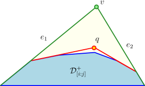
In particular, the query $q$ generated is inside $\pi$ and thus $C$. Contradicting that the recursive call was alive. It follows that each alive recursive call must contain at least one active edge. The number of active edges is bounded by $\left|{\pi}\right|$, implying the result.  

Lemma 4.4.

Let $C$ be a convex body provided via a separation oracle, and let $P$ be a set of $n$ points in the plane. The classification algorithm for reverse emptiness performs $O\bigl{(}\left|{F_{\mathrm{in}}}\right|\log n\bigr{)}$ oracle queries. The algorithm correctly verifies that $P\cap C=P$ or finds a witness point of $P$ outside $C$.

Proof:

Suppose all points of $P$ are inside $C$. By Lemma 4.3, there are at most $O(\left|{F_{\mathrm{in}}}\right|)$ alive recursive calls at each level of the recursion tree. Since the depth of the recursion tree is $O(\log n)$, the number of total alive recursive calls throughout the algorithm is $O(\left|{F_{\mathrm{in}}}\right|\log n)$. At each alive recursive call of the above algorithm, $O(1)$ queries are made. This implies the result.

Otherwise not all points of $P$ are inside $C$. At least one such point outside of $C$ must be a vertex on the convex hull $\mathcal{D}$. Hence after at most $O(\left|{F_{\mathrm{in}}}\right|\log n)$ oracle queries, this vertex will be queried and found to be outside $C$.  

5 Application: Minimizing a convex function

Suppose we are given a set of $n$ points $P$ in the plane and a convex function $f:\mathbb{R}^{2}\to\mathbb{R}$. Our goal is to compute the point in $P$ minimizing $\min_{p\in P}f(p)$. Given a point $p\in\mathbb{R}^{2}$, assuming that we can evaluate $f$ and the derivative of $f$ at $p$ efficiently, we show that the point in $P$ minimizing $f$ can be computed using $O(\varhexagon_{P}\log^{2}n)$ evaluations to $f$ or its derivative.

Definition 5.1.

Let $f:\mathbb{R}^{d}\to\mathbb{R}$ be a convex function. For a number $c\in\mathbb{R}$, define the level set of $f$ as $\mathcal{L}_{f}\left({c}\right)=\left\{p\in\mathbb{R}^{d}\;\middle|\;f(p)\leq c\right\}$. If $f$ is a convex function, then $\mathcal{L}_{f}\left({c}\right)$ is a convex set for all $c\in\mathbb{R}$.

Definition 5.2.

Let $f:\mathbb{R}^{d}\to\mathbb{R}$ be a convex (and possibly non-differentiable) function. For a point $p\in\mathbb{R}^{d}$, a vector $v\in\mathbb{R}^{d}$ is a subgradient of $f$ at $p$ if for all $q\in\mathbb{R}^{d}$, $f(q)\geq f(p)+\left\langle v,q-p\right\rangle$. The subdifferential of $f$ at $p\in\mathbb{R}^{d}$, denoted by $\partial f(p)$, is the set of all subgradients $v\in\mathbb{R}^{d}$ of $f$ at $p$.

It is well known that when the domain for $f$ is $\mathbb{R}^{d}$ and $f$ is a convex function, then $\partial f(p)$ is a non-empty set of all $p\in\mathbb{R}^{d}$ (for example, see [Fer13, Chapter 3]).

Let $\alpha=\min_{p\in P}f(p)$. We have that $\mathcal{L}_{f}\left({\alpha}\right)\cap P=\left\{p\in P\;\middle|\;f(p)=\alpha\right\}$ and $\mathcal{L}_{f}\left({\alpha^{\prime}}\right)\cap P=\varnothing$ for all $\alpha^{\prime}<\alpha$. Hence, the problem is reduced to determining the smallest value $r$ such that $\mathcal{L}_{f}\left({r}\right)\cap P$ is non-empty.

Lemma 5.3.

Let $P$ be a collection of $n$ points in the plane. For a given value $r$, let $C_{r}=\mathcal{L}_{f}\left({r}\right)$. The set $C_{r}\cap P$ can be computed using $O(\varhexagon_{P}\log n)$ evaluations to $f$ or its derivative. If $T$ is the time needed to evaluate $f$ or its derivative, the algorithm can be implemented in $O(n\log^{2}n\log\log n+T\cdot\varhexagon_{P}\log n)$ expected time.

Proof:

The Lemma follows by applying Theorem 2.8. Indeed, let $C_{r}=\mathcal{L}_{f}\left({r}\right)$ be the convex body of interest. It remains to design a separation oracle for $C_{r}$.

Given a query point $q\in\mathbb{R}^{2}$, first compute $c=f(q)$. If $c\leq r$, then report that $q\in C_{r}$. Otherwise, $c>r$. In this case, compute some gradient vector $v$ in $\partial f(q)$. Using the vector $v$, we can obtain a line $\mathcalb{l}$ tangent to the boundary of $\mathcal{L}_{f}\left({c}\right)$ at $q$. As $\mathcal{L}_{f}\left({r}\right)\subseteq\mathcal{L}_{f}\left({c}\right)$, $\mathcalb{l}$ is a separating line for $q$ and $C_{r}$, as desired. As such, the number of separation oracle queries needed to determine $C_{r}\cap P$ is bounded by $O(\varhexagon_{P}\log n)$ by Theorem 2.8.

The implementation details of Theorem 2.8 are given in Lemma 2.9.  

The algorithm.

Let $\alpha=\min_{p\in P}f(p)$. For a given number $r\geq 0$, set $P_{r}=\mathcal{L}_{f}\left({r}\right)\cap P$. We develop a randomized algorithm to compute $\alpha$.

Set $P_{0}=P$. In the $i$th iteration, the algorithm chooses a random point $p_{i}\in P_{i-1}$ and computes $r_{i}=f(p_{i})$. Next, we determine $P_{r_{i}}$ using Lemma 5.3. In doing so, we modify the separation oracle of Lemma 5.3 to store the collection of queries $S_{i}\subseteq P$ that satisfy $f(s)=r_{i}$ for all $s\in S_{i}$. We set $P_{i+1}=P_{r_{i}}\setminus S_{i}$. Observe that all points $p\in P_{i+1}$ have $f(p)<r_{i}$. The algorithm continues in this fashion until we reach an iteration $j$ in which $\left|{P_{j+1}}\right|\leq 1$. If $P_{j+1}=\{q\}$ for some $q\in P$, output $q$ as the desired point minimizing $f$. Otherwise $P_{j+1}=\varnothing$, implying that $P_{r_{j}}=S_{j}$, and the algorithm outputs any point in the set $S_{j}$.

Analysis.

We analyze the running time of the algorithm. To do so, we argue that the algorithm invokes the algorithm in Lemma 5.3 only a logarithmic number of times.

Lemma 5.4.

In expectation, the above algorithm terminates after $O(\log n)$ iterations.

Proof:

Let $V=\left\{f(p)\;\middle|\;p\in P\right\}$ and $N=\left|{V}\right|$. For a number $r$, define $V_{r}=\left\{i\in V\;\middle|\;i\leq r\right\}$. Notice that we can reinterpret the algorithm described above as the following random process. Initially set $r_{0}=\max_{i\in V}i$. In the $i$th iteration, choose a random number $r_{i}\in V_{r_{i-1}}$. This process continues until we reach an iteration $j$ in which $\left|{V_{r_{j}}}\right|\leq 1$.

We can assume without loss of generality that $V=\{1,2,\ldots,N\}$. For an integer $i\leq N$, let $T(i)$ be the expected number of iterations needed for the random process to terminate on the set $\{1,\ldots,i\}$. We have that $T(i)=1+\frac{1}{i-1}\sum_{j=1}^{i-1}T(i-j)$, with $T(1)=0$. This recurrence solves to $T(i)=O(\log i)$. As such, the algorithm repeats this random process $O(\log N)=O(\log n)$ times in expectation.  

Lemma 5.5.

Let $P$ be a set of $n$ points in $\mathbb{R}^{2}$ and let $f:\mathbb{R}^{2}\to\mathbb{R}$ be a convex function. The point in $P$ minimizing $f$ can be computed using $O(\varhexagon_{P}\log^{2}n)$ evaluations to $f$ or its derivative. The bound on the number of evaluations holds in expectation. If $T$ is the time needed to evaluate $f$ or its derivative, the algorithm can be implemented in $O(n\log^{3}n\log\log n+T\cdot\varhexagon_{P}\log^{2}n)$ expected time.

Proof:

The result follows by combining Lemma 5.3 and Lemma 5.4.  

5.1 The discrete geometric median

Let $P$ be a set of $n$ points in $\mathbb{R}^{d}$. For all $x\in\mathbb{R}^{d}$, define the function $f(x)=\sum_{q\in P-x}\|x-q\|_{2}$. The discrete geometric median is defined as the point in $P$ minimizing the quantity $\min_{p\in P}f(p)$.

Note that $f$ is convex, as it is the sum of convex functions. Furthermore, given a point $p$, we can compute $f(p)$ and the derivative of $f$ at $p$ in $O(n)$ time. As such, by Lemma 5.5, we obtain the following.

Lemma 5.6.

Let $P$ be a set of points in $\mathbb{R}^{2}$. Then the discrete geometric median of $P$ can be computed in $O(n\log^{2}n\cdot(\log n\log\log n+\varhexagon_{P}))$ expected time.

Remark 5.7.

For a set of $n$ points $P$ chosen uniformly at random from the unit square, it is known that in expectation $\varhexagon_{P}=\Theta(n^{1/3})$ [AB09]. As such, the discrete geometric median for such a random set $P$ can be computed in $O(n^{4/3}\log^{2}n)$ expected time.

6 Conclusion and open problems

In this paper we presented various algorithms for classifying points with oracle access to an unknown convex body. As far as the authors are aware, this exact problem has not been studied within the computational geometry community previously. However, since the problem is closely related to active learning and has further applications (such as discretely minimizing a convex function), we believe that this is an interesting problem to study. We now pose some open problems.

1. Develop a more natural instance-optimal algorithm in 2D that improves upon the $O(\log^{2}n)$ approximation. Alternatively, develop algorithms in which the number of queries is parameterized by different functions of the input instance.

2. An algorithm in 3D that is instance-optimal up to some additional factors (see the beginning of Appendix A for the definition of the separation price in higher dimensions).

3. Any results beyond three dimensions is unknown. The greedy algorithm (Theorem 2.8 and Theorem 2.19) easily extends to $\mathbb{R}^{d}$. However the analysis in higher dimensions will most likely reveal that the algorithm makes (ignoring logarithmic factors) of the order of ${\varhexagon_{P}}^{O(d)}$ queries, which is only interesting when $\varhexagon_{P}$ is much smaller than $n$.

4. In Lemma 5.6 we gave a randomized algorithm for computing the discrete geometric median in expected time $\widetilde{O}(n\cdot\varhexagon_{P})$ (where $\widetilde{O}$ hides logarithmic factors in $n$). The bottleneck of the algorithm was in the computation of the function and the gradient, which naively requires $O(n)$ time. Is it possible to speed up the gradient computation by introducing additional randomization or optimization techniques? Improving the running time further is an open problem.

Appendix A Expected separation price for random points

We first extend the notion of separation price (see Section 3.1) to higher dimensions. For a closed convex $d$-dimensional polytope $F$, we let $f_{k}(F)$ denote the number of $k$-dimensional faces of $F$.

Definition A.1 (Separation price in higher dimensions).

Let $P$ be a set of points and $C$ be a convex body in $\mathbb{R}^{d}$. The inner fence $F_{\mathrm{in}}$ is a closed convex $d$-dimensional polytope with the minimum number of vertices, such that $F_{\mathrm{in}}\subseteq C$ and $C\cap P=F_{\mathrm{in}}\cap P$. Similarly, the outer fence $F_{\mathrm{out}}$ is a closed convex $d$-dimensional polytope with the minimum number of facets, such that $C\subseteq F_{\mathrm{out}}$ and $C\cap P=F_{\mathrm{out}}\cap P$. The separation price is defined as $\varocircle\left({P,C}\right)=f_{0}(F_{\mathrm{in}})+f_{d-1}(F_{\mathrm{out}})$.

By extending the argument of Lemma 3.1 to use Definition A.1, one can prove the following.

Lemma A.2.

Given a point set $P$ and a convex body $C$ in $\mathbb{R}^{d}$, any algorithm that classifies the points of $P$ in relation to $C$, must perform at least $\varocircle\left({P,C}\right)$ separation oracle queries.

Informally, for any fixed convex body $C$ and a set of $n$ points $P$ chosen uniformly at random from the unit cube, the separation price is sublinear (approaching linear as the dimension increases).

Lemma A.3.

Let $P$ be a set of $n$ points chosen uniformly at random from the unit cube $[0,1]^{d}$, and let $C$ be a convex body in $\mathbb{R}^{d}$, with $\textsf{vol}(C)\geq c$ for some constant $c\leq 1$. Then $\mathop{\mathbf{E}}\!\left[{\varocircle\left({P,C}\right)}\right]=O(n^{1-2/(d+1)})$, where $O$ hides constants that depend on $d$ and $C$.

Proof:

It is known that for convex bodies $C$, the expected number of vertices of the convex hull of $P\cap C$ is $O(n^{1-2/(d+1)})$. Indeed, since $\textsf{vol}(C)\geq c$, the expected number of points of $P$ that fall inside $C$ is $m=\Theta(n)$ (and these bounds hold with high probability by applying any Chernoff-like bound). It is known that for $m$ points chosen uniformly at random from $C$, the expected size of the convex hull of points inside $C$ is $O(m^{1-2/(d+1)})=O(n^{1-2/(d+1)})$ [Wei07]. This readily implies that $\mathop{\mathbf{E}}\!\left[{f_{0}(F_{\mathrm{in}})}\right]=O(n^{1-2/(d+1)})$.

To bound $\mathop{\mathbf{E}}\!\left[{f_{d-1}(F_{\mathrm{out}})}\right]$, we apply a result of Dudley [Dud74] which states the following. Given a convex body $C$ and a parameter $\varepsilon>0$, there exists a convex body $D$, which is a polytope formed by the intersection of $O(\varepsilon^{-(d-1)/2})$ halfspaces, such that $C\subseteq D\subseteq(1+\varepsilon)C$, where $(1+\varepsilon)C=\left\{p\in\mathbb{R}^{d}\;\middle|\;\exists q\in C:\|p-q\|\leq\varepsilon\right\}$.

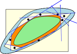
We claim that the number of points of $P$ that fall inside $D\setminus C$, plus the number of halfspaces defining $D$, is an upper bound on the size of the outer fence. Indeed, for each point $p$ that falls in inside $D\setminus C$, let $q$ be its nearest neighbor in $C$ (naturally $q$ lies on $\partial C$). Let $\mathcalb{h}_{p}$ be the hyperplane that is perpendicular to the segment $pq$ and passing through the midpoint of $pq$. Next, let $\mathcalb{h}^{+}_{p}$ be the halfspace bounded by $\mathcalb{h}_{p}$ such that $C\subseteq\mathcalb{h}^{+}_{p}$. If $H$ is the collection of $O(\varepsilon^{-(d-1)/2})$ halfspaces defining $D$, then it is easy to see that the polytope defined by

$$\Bigl{(}{\bigcap_{p\in P\cap(D\setminus C)}\mathcalb{h}^{+}_{p}}\Bigr{)}\hskip 0.6pt\bigcap\,\Bigl{(}{\bigcap_{\mathcalb{h}^{+}\in H}\mathcalb{h}^{+}}\Bigr{)}$$

separates the boundary of $C$ from $P\setminus C$ (i.e., it is an outer fence). See Figure A.1.

Figure A.1:

We now bound the size of this inner fence. Since $\textsf{vol}(D)-\textsf{vol}(C)\leq\textsf{vol}((1+\varepsilon)C)-\textsf{vol}(C)\leq O(\varepsilon)$, we have that $\mathop{\mathbf{E}}\!\left[{\left|{P\cap(D\setminus C)}\right|}\right]=O(\varepsilon n)$. Combining both inequalities,

$$\mathop{\mathbf{E}}\!\left[{f_{d-1}(F_{\mathrm{out}})}\right]\leq\mathop{\mathbf{E}}\!\left[{\left|{P\cap(D\setminus C)}\right|}\right]+O(\varepsilon^{-(d-1)/2})=O\left({\varepsilon n+\frac{1}{\varepsilon^{(d-1)/2}}}\right).$$

Choose $\varepsilon=1/n^{2/(d+1)}$ to balance both terms, so that $\mathop{\mathbf{E}}\!\left[{f_{d-1}(F_{\mathrm{out}})}\right]=O(n^{1-2/(d+1)})$.  

The next Lemma shows that the bound of Lemma A.3 is tight in the worst case.

Lemma A.4.

Let $P$ be a set of $n$ points chosen uniformly at random from the hypercube $[-2,2]^{d}$, and let $C$ be a unit radius ball centered at the origin. Then $\mathop{\mathbf{E}}\!\left[{\varocircle\left({P,C}\right)}\right]\geq\mathop{\mathbf{E}}\!\left[{f_{0}(F_{\mathrm{in}})}\right]=\Omega(n^{1-2/(d+1)})$, where $\Omega$ hides constants depending on $d$.

Proof:

For a parameter $\delta$ to be chosen, let $Q\subseteq\partial C$ be a maximal set of points such that:

1. for any $p\in\partial C$, there is a point $q\in Q$ such that $\|p-q\|\leq\delta$, and

2. for any two points $p,q\in Q$, $\|p-q\|\geq\delta$.

Note that $\left|{Q}\right|=\Omega(1/\delta^{d-1})$. For each $p\in Q$, we let $\gamma_{p}$ be the spherical cap that is “centered” at $p$ (in the sense that the center of the base of $\gamma_{p}$, $p$, and the origin are collinear) and has base radius $2\delta$. Let $\Gamma=\left\{\gamma_{p}\;\middle|\;p\in Q\right\}$. By construction, the caps of $\Gamma$ cover the surface of $C$.

By setting $\delta=1/n^{1/(d+1)}$, we claim that for each cap $\gamma\in\Gamma$, in expectation $\Omega(1)$ points of $P$ fall inside $\gamma$. This implies that there must be a vertex of the inner fence inside $\gamma$, and this holds for all caps in $\Gamma$. As such, the size of the inner fence is at least $\left|{Q}\right|=\Omega(1/\delta^{d-1})=\Omega(n^{1-2/(d+1)})$.

Figure A.2:

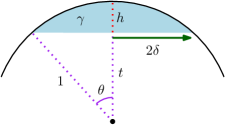
To prove the claim, for all $\gamma\in\Gamma$, we show that $\textsf{vol}(\gamma)=\Omega(1/n)$, and hence $\mathop{\mathbf{E}}\!\left[{\left|{P\cap\gamma}\right|}\right]=\Omega(1)$. By construction, the cap has a polar angle of $\theta=\Omega(\delta)$, see Figure A.2. Indeed, we have that $\theta\geq\sin(\theta)=2\delta$ for $\theta\in[0,\pi/2]$ (which holds when $n$ is sufficiently large). Let $t$ denote the distance from the origin to the center of the base of $\gamma$. Then the height $h$ of the spherical cap is $h=1-t=1-\cos(\theta)\geq\theta^{2}/6=\Omega(\delta^{2})$ (using the inequality $\cos(x)\leq 1-x^{2}/6$). Since the volume of the base of $\gamma$ is $\Omega(\delta^{d-1})$, we have that $\textsf{vol}(\gamma)=\Omega(h\delta^{d-1})=\Omega(\delta^{d+1})=\Omega(1/n)$, as required.

References

- [AB09] G. Ambrus and I. Bárány “Longest convex chains” In Rand. Struct. & Alg. 35.2, 2009, pp. 137–162 DOI: 10.1002/rsa.20269
- [Ang87] Dana Angluin “Queries and Concept Learning” In Machine Learning 2.4, 1987, pp. 319–342 DOI: 10.1007/BF00116828
- [Bár82] I. Bárány “A generalization of Carathéodory’s theorem” In Discrete Math. 40.2-3 Elsevier, 1982, pp. 141–152 DOI: 10.1016/0012-365X(82)90115-7
- [BF87] Imre Bárány and Zoltán Füredi “Computing the Volume is Difficulte” In Discrete Comput. Geom. 2, 1987, pp. 319–326 DOI: 10.1007/BF02187886
- [CAL94] David A. Cohn, Les E. Atlas and Richard E. Ladner “Improving Generalization with Active Learning” In Machine Learning 15.2, 1994, pp. 201–221 DOI: 10.1007/BF00993277
- [Cha04] T.. Chan “An optimal randomized algorithm for maximum Tukey depth” In Proc. 15th ACM-SIAM Sympos. Discrete Algs. (SODA) SIAM, 2004, pp. 430–436 URL: http://dl.acm.org/citation.cfm?id=982792.982853
- [CLM+16] Michael B. Cohen et al. “Geometric median in nearly linear time” In Proc. 48th ACM Sympos. Theory Comput. (STOC) ACM, 2016, pp. 9–21 DOI: 10.1145/2897518.2897647
- [CS89] K.. Clarkson and P.. Shor “Applications of random sampling in computational geometry, II” In Discrete Comput. Geom. 4, 1989, pp. 387–421 DOI: 10.1007/BF02187740
- [Dud74] R.. Dudley “Metric entropy of some classes of sets with differentiable boundaries” In J. Approx. Theory 10.3, 1974, pp. 227–236 DOI: https://doi.org/10.1016/0021-9045(74)90120-8
- [ES19] Esther Ezra and Micha Sharir “A Nearly Quadratic Bound for Point-Location in Hyperplane Arrangements, in the Linear Decision Tree Model” In Discrete Comput. Geom. 61.4, 2019, pp. 735–755 DOI: 10.1007/s00454-018-0043-8
- [Fer13] Juan Ferrera “An introduction to nonsmooth analysis” Boston: Academic Press, 2013 DOI: 10.1016/C2013-0-15234-8
- [GG07] Yuhong Guo and Russell Greiner “Optimistic Active-Learning Using Mutual Information” In Proc. 20th Int. Joint Conf. on AI (IJCAI), 2007, pp. 823–829 URL: http://ijcai.org/Proceedings/07/Papers/132.pdf
- [HJR18] S. Har-Peled, M. Jones and S. Rahul “An animation of the greedy classification algorithm in 2D” https://www.youtube.com/watch?v=IZX0VQdIgNA, 2018 Youtube URL: https://www.youtube.com/watch?v=IZX0VQdIgNA
- [HJR20] Sariel Har-Peled, Mitchell Jones and Saladi Rahul “Active Learning a Convex Body in Low Dimensions” In Proc. 47th Int. Colloq. Automata Lang. Prog. (ICALP) 168, Leibniz International Proceedings in Informatics (LIPIcs) Dagstuhl, Germany: Schloss Dagstuhl–Leibniz-Zentrum für Informatik, 2020, pp. 64:1–64:17 DOI: 10.4230/LIPIcs.ICALP.2020.64
- [HKMR16] S. Har-Peled, N. Kumar, D.. Mount and B. Raichel “Space Exploration via Proximity Search” In Discrete Comput. Geom. 56.2, 2016, pp. 357–376 DOI: 10.1007/s00454-016-9801-7
- [HW87] David Haussler and Emo Welzl “-Nets and Simplex Range Queries” In Discrete & Computational Geometry 2, 1987, pp. 127–151 DOI: 10.1007/BF02187876
- [KLMZ17] Daniel M. Kane, Shachar Lovett, Shay Moran and Jiapeng Zhang “Active Classification with Comparison Queries” In Proc. 58th Annu. IEEE Sympos. Found. Comput. Sci. (FOCS), 2017, pp. 355–366 DOI: 10.1109/FOCS.2017.40
- [KLPS86] K. Kedem, R. Livne, J. Pach and M. Sharir “On the union of Jordan regions and collision-free translational motion amidst polygonal obstacles” In Discrete Comput. Geom. 1.1 Springer, 1986, pp. 59–71 DOI: 10.1007/BF02187683
- [Kup20] Andrey Kupavskii “The VC-dimension of k-vertex d-polytopes” In CoRR abs/2004.04841, 2020 arXiv: https://arxiv.org/abs/2004.04841
- [Mat02] J. Matoušek “Lectures on Discrete Geometry” 212, Grad. Text in Math. Springer, 2002 DOI: 10.1007/978-1-4613-0039-7/
- [MN90] Kurt Mehlhorn and Stefan Näher “Dynamic Fractional Cascading” In Algorithmica 5.2, 1990, pp. 215–241 DOI: 10.1007/BF01840386
- [MW03] J. Matoušek and U. Wagner “New constructions of weak epsilon-nets” In Proceedings of the nineteenth annual symposium on Computational geometry, 2003, pp. 129–135 ACM
- [PASG13] F. Panahi, A. Adler, A.. Stappen and K. Goldberg “An efficient proximity probing algorithm for metrology” In Int. Conf. on Automation Science and Engineering, CASE 2013, 2013, pp. 342–349 DOI: 10.1109/CoASE.2013.6653995
- [PS85] Franco P. Preparata and Michael Ian Shamos “Computational Geometry - An Introduction”, Texts and Monographs in Computer Science Springer, 1985 DOI: 10.1007/978-1-4612-1098-6
- [Rub18] Natan Rubin “An Improved Bound for Weak Epsilon-Nets in the Plane” In Proc. 59th Annu. IEEE Sympos. Found. Comput. Sci. (FOCS) IEEE Computer Society, 2018, pp. 224–235 DOI: 10.1109/FOCS.2018.00030
- [Set09] Burr Settles “Active Learning Literature Survey”, 2009 URL: https://minds.wisconsin.edu/bitstream/handle/1793/60660/TR1648.pdf?sequence=1&isAllowed=y
- [VC71] V.. Vapnik and A.. Chervonenkis “On the uniform convergence of relative frequencies of events to their probabilities” In Theory Probab. Appl. 16, 1971, pp. 264–280
- [Wei07] “Random Polytopes, Convex Bodies, and Approximation” In Stochastic Geometry: Lectures given at the C.I.M.E. Summer School held in Martina Franca, Italy, September 13–18, 2004 Berlin, Heidelberg: Springer Berlin Heidelberg, 2007, pp. 77–118 DOI: 10.1007/978-3-540-38175-4˙2