University of Southampton

Faculty of Engineering and Physical Sciences

Department of Physics and Astronomy

 

Recurrent Instability in LMXB Accretion Disks: How Strange is GRS 1915+105?

 

Author
James Matthew Christopher Court
ORCID ID 0000-0002-0873-926X
Thesis for the degree of
Doctor of Philosophy

Abstract

Low Mass X-Ray Binaries (LMXBs) are systems in which a black hole or neutron star accretes matter from a stellar binary companion. The accreted matter forms a disk of material around the compact object, known as an accretion disk. The X-ray properties of LMXBs show strong variability over timescales ranging from milliseconds to decades. Many of these types of variability are tied to the extreme environment of the inner accretion disk, and hence an understanding of this behaviour is key to understanding how matter behaves in such an environment. GRS 1915+105 and MXB 1730-335 (also known as the Rapid Burster) are two LMXBs which show particularly unusual variability. GRS 1915+105 shows a large number of distinct ‘classes’ of second-to-minute scale variability, consisting of repeated patterns of dips and flares. The Rapid Burster on the other hand shows ‘Type II X-ray Bursts’; second-to-minute scale increases in X-ray intensity with a sudden onset and a slower decay. For many years both of these objects were thought to be unique amongst all known LMXBs. More recently, two new objects, IGR J17091-3624 and GRO J1744-28 (also known as the Bursting Pulsar) have been shown to display similar behaviour to those seen in GRS 1915+105 and the Rapid Burster respectively.

In this thesis, I first present a new framework with which to classify variability seen in IGR J17091-3624. Using my set of independent variability classes constructed for IGR J17091-3624, I perform a study of the similarities and differences between this source and GRS 1915+105 to better constrain their underlying physics. In GRS 1915, hard X-ray emission lags soft X-ray emission in all variability classes; in IGR J17091, I find that the sign of this lag is different in variability classes. Additionally, while GRS 1915+105 accretes at close to its Eddington Limit, I find that IGR J17091-3624 accretes at only $\sim 5$–33% of its Eddington Limit. With these results I rule out any models which require near-Eddington accretion or hard corona reacting to the disk. I also perform a study of the variability seen in the Bursting Pulsar. I find that the flaring behaviour in the Bursting Pulsar is significantly more complex than in the Rapid Burster, consisting of at least 4 separate phenomena which may have separate physical origins. One of these phenomena, ‘Structured Bursting’, consists of patterns of flares and dips which are similar to those seen in GRS 1915+105 and IGR J17091-3624. I compare these two types of variability and discuss the possibility that they are caused by the same physical instability. I also present the alternative hypothesis that Structured Bursting is a manifestation of ‘hiccup’ variability; a bimodal flickering of the accretion rate seen in systems approaching the ‘propeller’ regime.

Contents

1. Abstract
2. Dedication
3. Acknowledgements
4. Declaration of Authorship
5. 1 Introduction
   1. 1.1 Anatomy of an X-Ray Binary
      1. 1.1.1 Types of X-Ray Binaries: High and Low-Mass
      2. 1.1.2 Components of a Low Mass X-Ray Binary
   2. 1.2 Low Mass X-Ray Binary Behaviour
   3. 1.3 Relativistic Effects
6. 2 The Physics of Accretion
   1. 2.1 The Shakura-Sunyaev Disk Model
      1. 2.1.1 The source of Turbulence
   2. 2.2 Accretion Phenomena
      1. 2.2.1 The Eddington Limit
      2. 2.2.2 The Propeller Effect
      3. 2.2.3 Disk Instabilities
   3. 2.3 GRS 1915+105 and IGR J17091-3624
      1. 2.3.1 A History of Models of GRS 1915-like Variability
   4. 2.4 Type II Burst Sources
      1. 2.4.1 A History of Models of Type II Bursts
7. 3 Tools & Methods
   1. 3.1 Instrumentation
      1. 3.1.1 The Rossi X-Ray Timing Experiment
      2. 3.1.2 The Neil Gehrels Swift Observatory
      3. 3.1.3 The X-Ray Multi-Mirror Mission
      4. 3.1.4 Chandra
      5. 3.1.5 Suzaku
      6. 3.1.6 The Nuclear Spectroscopic Telescope Array
      7. 3.1.7 The International Gamma-Ray Astrophysics Laboratory
      8. 3.1.8 Dead-time and Pile-up
   2. 3.2 Methods & Techniques
      1. 3.2.1 Lightcurve Morphology
      2. 3.2.2 Timing Analysis
      3. 3.2.3 Energy Spectral Analysis
8. 4 Variability in IGR J17091-3624: Classification
   1. 4.1 Data and Data Analysis
      1. 4.1.1 RXTE
      2. 4.1.2 Swift
      3. 4.1.3 INTEGRAL
      4. 4.1.4 XMM-Newton
      5. 4.1.5 Chandra
      6. 4.1.6 Suzaku
   2. 4.2 Results
      1. 4.2.1 Outburst Evolution
      2. 4.2.2 RXTE
      3. 4.2.3 Swift
      4. 4.2.4 INTEGRAL
      5. 4.2.5 Chandra
      6. 4.2.6 XMM-Newton
      7. 4.2.7 Suzaku
   3. 4.3 Discussion
      1. 4.3.1 Variability Classes: IGR J17091 vs. GRS 1915
      2. 4.3.2 General Comparison with GRS 1915+105
      3. 4.3.3 Comparison with the Rapid Burster
      4. 4.3.4 Comparison with Altamirano et al., 2011b,
      5. 4.3.5 New Constraints on Accretion Rate, Mass & Distance
      6. 4.3.6 Implications for Models of ‘Heartbeat’ Variability
   4. 4.4 Conclusions
9. 5 The Evolution of X-ray Bursts in the ‘Bursting Pulsar’ GRO J1744–28
   1. 5.1 Data and Data Analysis
      1. 5.1.1 RXTE
      2. 5.1.2 Swift
      3. 5.1.3 INTEGRAL
      4. 5.1.4 Chandra
      5. 5.1.5 XMM-Newton
      6. 5.1.6 Suzaku
      7. 5.1.7 NuSTAR
   2. 5.2 Results
      1. 5.2.1 Outburst Evolution
      2. 5.2.2 Categorizing Bursts
      3. 5.2.3 Normal Bursts
      4. 5.2.4 Minibursts
      5. 5.2.5 Mesobursts
      6. 5.2.6 Structured ‘Bursts’
   3. 5.3 Discussion
      1. 5.3.1 Evolution of Outburst and Bursting Behaviour
      2. 5.3.2 Parameter Correlations
      3. 5.3.3 Comparison with Previous Studies
      4. 5.3.4 Comparison with other objects
      5. 5.3.5 Comparison with Models of Type II Bursts
   4. 5.4 Conclusions
10. 6 The Bursting Pulsar GRO J1744-28: the Slowest Transitional Pulsar?
    1. 6.1 Transitional Millisecond Pulsars
    2. 6.2 Comparison: TMSPs vs. the Bursting Pulsar
    3. 6.3 Discussion
       1. 6.3.1 Comparison with other Objects
    4. 6.4 Conclusion
11. 7 Discussion
    1. 7.1 General Observations
       1. 7.1.1 Variability Evolution throughout an Ouburst
       2. 7.1.2 Criteria for Exotic Variability
       3. 7.1.3 Evidence of System Memory
    2. 7.2 IGR J17091 vs. the Bursting Pulsar: A Comparison
       1. 7.2.1 Variability Classes and Burst Classes
       2. 7.2.2 Structured Bursting
    3. 7.3 Future Research
12. 8 Conclusions
13. A Model-Independent Classification of each Observation of IGR J17091-3624
14. B List of RXTE Observations of the Bursting Pulsar
15. C Normal Burst Histograms
16. D PANTHEON suite
    1. D.1 FITS Genie
    2. D.2 Plot Demon
    3. D.3 Spec Angel
    4. D.4 Back Hydra
    5. D.5 PAN Lib

List of Figures

1. 1.1 A cartoon illustrating the basic geometry of a simple X-ray binary.
2. 1.2 A series of 5 GHz radio images from Fender et al., (1999) showing a jet being launched from the LMXB GRS 1915+105.
3. 1.3 Two simulated, simplified spectra of an LMXB, showing the two main components visible in X-ray: the accretion disk and the corona.
4. 1.4 A schematic hardness-intensity diagram adapted from Fender et al., (2004), showing the evolutionary path of a typical black hole LMXB outburst.
5. 1.5 Energy spectra of the black hole HMXB Cygnus X-1 in its low/hard and high/soft states, presented as typical spectra of a black hole XRB in these states.
6. 1.6 Colour-Colour diagrams from van der Klis, 1989b showing typical evolutionary paths of Atoll-type and Z-type Neutron Star LMXBs.
7. 2.1 Diagrams showing the path of an element of gas in a neutron star accretion disk for different arrangements of the corotation and magnetospheric radii.
8. 2.2 Typical lightcurves of a selection of variability classes seen in the LMXB GRS 1915+105.
9. 2.3 A schematic diagram illustrating the the process described by Neilsen et al., (2011) to describe the $\rho$ variability class in GRS 1915+105.
10. 2.4 An RXTE/PCA lightcurve of the Rapid Burster, showing a number of typical Type II X-ray bursts.
11. 3.1 A cartoon illustrating the process of folding a periodic lightcurve with a known period.
12. 3.2 A cartoon illustrating the procedure of the algorithm described in Section .
13. 3.3 A representation of how a continuous variable is convolved with a windowing function and a sampling function to yield physical data.
14. 3.4 Hardness-Intensity diagrams of black bodies with temperatures and normalisations described by various functional forms.
15. 4.1 Lightcurves of IGR J17091-3624, from a number of instruments, during its 2011-2013 outburst.
16. 4.2 Lightcurves of IGR J17091-3524 during the 2011-2013 outburst, showing when each of variability classes I-IX were observed.
17. 4.3 Hardness-Intensity diagrams of IGR J17091-3524 during the 2011-2013 outburst, showing when each of variability classes I-IX were observed.
18. 4.4 Characteristic lightcurves and a power spectrum of Type I variability.
19. 4.5 Characteristic lightcurves and a power spectrum of Type II variability.
20. 4.6 Characteristic lightcurves and a power spectrum of Type III variability.
21. 4.7 The Lomb-Scargle periodogram of Class III observation 96420-01-19-01
22. 4.8 A hardness-intensity diagram of the Class III observation 96420-01-04-01.
23. 4.9 Characteristic lightcurves and a power spectrum of Type IV variability.
24. 4.10 The hardness-intensity diagram of the Class IV observation 96420-01-05-00, showing an anticlockwise loop.
25. 4.11 Characteristic lightcurves and a power spectrum of Class V variability.
26. 4.12 A portion of the lightcurve of observation 96420-01-06-03 showing Type $V_{1}$ flares and Type $V_{2}$ flares.
27. 4.13 Every flare in all observations identified as Class V, plotted in a two-dimensional histogram of flare peak count rate against flare duration to show the two-population nature of these events.
28. 4.14 The hardness-intensity diagram of a type $V_{1}$ flaring period in Class V observation 96420-01-07-00 showing a clockwise loop.
29. 4.15 Characteristic lightcurves and a power spectrum of Type VI variability.
30. 4.16 The hardness-intensity diagram of the Class VI observation 96420-01-30-03, showing a clockwise loop.
31. 4.17 Characteristic lightcurves and a power spectrum of Type VII variability.
32. 4.18 A sliding window Lomb-Scargle spectrogram of Class VII observation 96420-01-18-05.
33. 4.19 Characteristic lightcurves and a power spectrum of Type VIII variability.
34. 4.20 Characteristic lightcurves and a power spectrum of Type IX variability.
35. 4.21 INTEGRAL/ISGRI 150–300 keV significance map of a $2^{\circ}$ region centred on the position of IGR J17091-3624.
36. 4.22 Chandra lightcurves showing examples of Class I, VII and IX variability.
37. 4.23 XMM-Newton lightcurves showing an example of Class IV variability and the hard state.
38. 4.24 $\nu P(\nu)$-normalised co-added power density spectra of XMM-Newton observation 0700381301 and Suzaku observation 407037010.
39. 4.25 A lightcurve of observation 96420-01-06-02, showing a transition in behaviour between Classes IV and V.
40. 4.26 Every flare in all observations identified as Class III or Class IV, plotted in a two-dimensional histogram of flare peak count rate against flare duration to show the two-population nature of these events.
41. 4.27 Lightcurve from Class III observation 96420-01-10-01 of IGR J17091-3624, with pairs of primary and secondary count rate spikes highlighted.
42. 4.28 Mass of the compact object in IGR J17091-3624 plotted against its distance, for values of peak Eddington fractions of $F_{Edd}=$0.05, 0.1, 0.2 and 0.33.
43. 5.1 Comparisons of three outbursts of the Bursting Pulsar.
44. 5.2 RXTE/PCA lightcurves of Outbursts 1 & 2 of the Bursting Pulsar, overlaid with plots showing how the fractional RMS of the 2.4 Hz pulsation changes as a function of time.
45. 5.3 Lightcurves for the four classes of bursting behaviour identified in the Bursting Pulsar.
46. 5.4 Histogram of the peak 1 s binned peak count rates during Normal Bursts, Mesobursts and Minibursts as seen by RXTE
47. 5.5 Lightcurve of the 1995–1996 outburst of the Bursting Pulsar, highlighting periods of time during which Mesobursts, Structured Bursts or Normal and Mini bursts are observed.
48. 5.6 Lightcurve of the 1997–1999 outburst of the Bursting Pulsar, highlighting periods of time during which Mesobursts, Structured Bursts or Normal and Mini bursts are observed.
49. 5.7 The distribution of recurrence times between consecutive Normal Bursts in Outburst 3.
50. 5.8 A plot of every Normal Burst, centred by the time of its peak, overlaid on top of each other to show the existence of a common pulse profile.
51. 5.9 RXTE lightcurves of Normal Bursts with (top) and without (bottom) ‘plateau’ features, showing the burst structure in each case.
52. 5.10 A schematic explaining the origin of the 12 Normal Burst parameters used in this study.
53. 5.11 Covariance Matrix with a scatter plot of each pairing of the 12 normalised Normal Burst parameters listed in section .
54. 5.12 A hardness-intensity diagram of a typical Normal Burst.
55. 5.13 A representative RXTE lightcurve of a Miniburst.
56. 5.14 A plot of every Miniburst, centred by the time of its peak, overlaid on top of each other.
57. 5.15 A portion of observation 10401-01-16-00, featuring a fNormal Burst and a Miniburst.
58. 5.16 A lightcurve from RXTE observation 20078-01-17-00 from Outburst 2, showing an apparent ‘plateau’ feature after a Mesoburst.
59. 5.17 A plot of every Mesoburst, centred by the time of its peak, overlaid on top of each other.
60. 5.18 A lightcurve from RXTE/PCA observation 10401-01-57-03, showing a Mesoburst occuring during a period of Structured Bursting.
61. 5.19 A hardness-intensity diagram from RXTE observation 20078-01-23-00, showing that hardness tends to correlate with intensity during Structured Bursting.
62. 5.20 A selection of RXTE lightcurves from Structured Bursting observations of the Bursting Pulsar.
63. 5.21 A series of lightcurves from RXTE/PCA observations of Outburst 2, showing a gradual evolution from Mesobursts to Structured Bursting over a period of $\sim 30$ days.
64. 5.22 RXTE lightcurves of representative Long (top) and Short (bottom) Type II bursts from the Rapid Burster.
65. 5.23 A scatter plot showing the relationship between burst fluence and ‘missing’ dip fluence for Normal Bursts and Minibursts.
66. 6.1 Lightcurves from the Bursting Pulsar and from two TMSPs, showing similar patterns of variability.
67. 6.2 Histograms of the 1 s binned count rates from all RXTE observations of Structured Bursting in the 1996 and 1997 outbursts of the Bursting Pulsar.
68. 6.3 A 7–60/2–7 keV hardness-intensity diagram for RXTE observation 10401-01-59-00 of the Bursting Pulsar.
69. 6.4 A plot of a number of objects ranging in scale from LMXBs and High-Mass X-ray Binaries (HMXBs) to Cataclysmic Variables (CVs) and Young Stellar Objects (YSOs). In each case, the object is plotted at the luminosity which defines its transition between propeller-mode accretion and free accretion.
70. 6.5 A plot of spin period against rate of spin-down for the population of all known radio pulsars, a so-called $P$–$\dot{P}$ diagram, showing where the Bursting Pulsar lies in this parameter space and indicating that it lies well outside of the pulsar ‘graveyard’.
71. 7.1 A Swift/XRT lightcurve of IGR J17091-3624 during its 2016 outburst, showing Class III variability.
72. 7.2 Lightcurves from GRS 1915, IGR J17091 and the Bursting Pulsar, showing lightcurves with Normal Burst-like behaviour for each.
73. 7.3 Lightcurves from GRS 1915, IGR J17091 and the Bursting Pulsar, showing lightcurves with Structured Bursting-like behaviour for each.
74. C.1 Histogram showing the distribution of $\phi_{B}$ amongst Normal Bursts.
75. C.2 Histogram showing the distribution of $a_{B}$ amongst Normal Bursts.
76. C.3 Histogram showing the distribution of $\sigma_{B}$ amongst Normal Bursts.
77. C.4 Histogram showing the distribution of $c$ amongst Normal Bursts.
78. C.5 Histogram showing the distribution of $\phi_{d}$ amongst Normal Bursts.
79. C.6 Histogram showing the distribution of $a_{d}$ amongst Normal Bursts.
80. C.7 Histogram showing the distribution of $d$ amongst Normal Bursts.
81. C.8 Histogram showing the distribution of $\lambda$ amongst Normal Bursts.
82. C.9 Histogram showing the distribution of $\phi_{p}$ amongst Normal Bursts.
83. C.10 Histogram showing the distribution of $a_{p}$ amongst Normal Bursts.
84. C.11 Histogram showing the distribution of $\phi_{B}/k$ amongst Normal Bursts.
85. C.12 Histogram showing the distribution of $a_{B}/k$ amongst Normal Bursts.
86. C.13 Histogram showing the distribution of $\phi_{d}/k$ amongst Normal Bursts.
87. C.14 Histogram showing the distribution of $a_{d}/k$ amongst Normal Bursts.
88. C.15 Histogram showing the distribution of $\phi_{p}/k$ amongst Normal Bursts.
89. C.16 Histogram showing the distribution of $a_{p}/k$ amongst Normal Bursts.

List of Tables

1. 4.1 Chandra observations log covering the three observations considered in Chapter 4.
2. 4.2 A number of statistics averaged across all observations belonging to each IGR J17091 variability class.
3. 4.3 A tally of the number of times I assigned each of my nine Variability Classes to an RXTE orbit observing IGR J17091.
4. 4.4 Results from the IBIS/ISGRI analysis of the 2011–2013 Outburst of IGR J17091.
5. 4.5 The nine variability classes of IGR J17091-3624, showing the name of the closest corresponding variability class in GRS 1915+105.
6. 4.6 The six IGR J17091-3624 ObsIDs explicitly classified in Altamirano et al., 2011b .
7. 5.1 Information on the three Chandra observations of the Bursting Pulsar during its 2014 outburst.
8. 5.2 Information on two NuSTAR observations of the Bursting Pulsar during its 2014 outburst.
9. 5.3 Statistics on the population of bursts in the 1996 and 1997 outbursts of the Bursting Pulsar.
10. 5.4 A table showing the mean and standard deviation of 10 Normal Burst parameters of RXTE-sampled bursts.
11. 5.5 A table showing the mean and standard deviation of 7 parameters of RXTE-sampled Minibursts from the 1996 outburst, the 1997 outburst and both outbursts combined.
12. 5.6 A table showing the mean and standard deviation of 7 burst parameters of RXTE-sampled Mesobursts from the 1996 & 1997 outbursts.
13. 5.7 A table showing how my burst classes for the Bursting Pulsar map to those described in Giles et al., (1996).
14. A.1 The variability class assigned to each RXTE observation of IGR J17091-3624 considered in this thesis.
15. A.2 A continuation of Table A.1. This table is continued overleaf in Tables A.3 and A.4.
16. A.3 A continuation of Table A.1. This table is continued overleaf in Table A.4.
17. A.4 A continuation of Table A.1.
18. B.1 A list of all RXTE observations of the Bursting Pulsar used in this thesis.
19. B.2 A continuation of Table B.1. This table is further continued in Table B.3.
20. B.3 A continuation of Table B.1.

Dedication

To the memory of my brother Christopher, whose name will forever appear alongside my own.

Declaration of Authorship

I, James Matthew Christopher Court, declare that this thesis entitled Recurrent Instability in LMXB Accretion Disks: How Strange is GRS 1915+105? and the work presented herein are my own and has been generated by me as the result of my own original research. I confirm that:

• This work was done wholly or mainly while in candidature for a research degree at this University;

• Where any part of this thesis has previously been submitted for a degree or any other qualification at this University or any other institution, this has been clearly stated;

• Where I have consulted the published work of others, this is always clearly attributed;

• Where I have quoted from the work of others, the source is always given. With the exception of such quotations, this thesis is entirely my own work;

• I have acknowledged all main sources of help;

• Where the thesis is based on work done by myself jointly with others, I have made clear exactly what was done by others and what I have contributed myself;

• Parts of this work have been published as:

  • Chapter 4: An atlas of exotic variability in IGR J17091-3624: a comparison with GRS 1915+105, 2017 MNRAS 468 4748-4771, hereafter Court et al., (2017).

  • Chapter 5: The Evolution of X-ray Bursts in the "Bursting Pulsar" GRO J1744-28, 2018 MNRAS 481 2273-2239, hereafter Court et al., 2018a .

  • Chapter 6: The Bursting Pulsar GRO J1744-28: the slowest transitional pulsar?, 2018 MNRASL 477 L106-L110, hereafter Court et al., 2018b .

Signed: ………………………………………

Date: ………………………………………..

Chapter 1 Introduction

Light thinks it travels faster than anything but it is wrong. No matter how fast light travels, it finds the darkness has always got there first, and is waiting for it.

Terry Pratchett – Reaper Man

In this thesis, I discuss the physics of matter in close proximity to neutron stars and black holes. These astrophysical entities, collectively referred to as ‘compact objects’, are the densest objects known to exist in our universe, and are formed in the death throes of massive stars.

When a star with a mass between $\sim 8$–10 $M_{\odot}$ (e.g. Bildsten and Strohmayer,, 1999) runs out of nuclear fuel in its core, it is no longer able to support its own weight and collapses inwards. This collapse generates a shockwave which disrupts the star, resulting in most of the star being ejected in an event known as a supernova. The core of the star survives this disruption and continues collapsing. The core of a massive star is supported by electron degeneracy pressure; a pressure caused by the fact that no two fermions can occupy the same quantum state (Pauli,, 1925). However, during the collapse of the core in a supernova, even electron degeneracy pressure cannot support the star; when the core has a mass greater than 1.4 M_⊙ (the Chandrasekhar Limit, Chandrasekhar,, 1931), electrons merge with protons via inverse $\beta$-decay, forming an object supported mostly by neutron degeneracy pressure. The resulting ‘neutron star’ is an extremely dense object, with a mass of several M_⊙ compressed into a sphere with a radius of $\sim 20$ km. Additionally as the core collapses, it spins up to conserve angular momentum until it is rotating at a rate of $\sim 100$ Hz. The extreme gravitational field in the proximity of such a strong object results in a region of space which is strongly affected by the effects predicted by general relativity (Einstein,, 1916). The extremely rapid rotation of neutron stars, and the associated high-velocity electron and proton populations present in their cores (e.g. Alpar and Sauls,, 1988), can result in magnetic fields as strong as $\sim 10^{15}$ G (Woltjer,, 1964; Gold,, 1968; Kaspi and Beloborodov,, 2017). For a collapsing star with a mass of greater than $\sim 10$ M$\odot$, the end product is even more extreme. The core of such a star can become so dense during a supernova that even neutron degeneracy pressure cannot support it, and instead it collapses into a black hole; a region of space with such a strong gravitational field that no information can escape it.

Unfortunately, compact objects are inherently faint objects. In fact, an isolated black hole is theoretically only visible via the effects its gravitational well has on the light from stars located behind it. As such, observational research into these objects tends to focus one of two types of system: Active Galactic Nuclei (AGN) and X-Ray Binaries (XRBs). In both of these types of system a compact object gravitationally attracts matter from its surrounding enviroment, a process known as ‘accretion’. The act of matter falling into such a steep gravitational well causes large amounts of energy to be released; as such, these systems shine brightly in high-energy regions of the electromagnetic spectrum such as the X-rays and $\gamma$-rays.

AGN contain supermassive black holes with masses upwards of $\sim 10^{6}$ $M_{\odot}$ (e.g. Miyoshi et al.,, 1995). These black holes are believed to be present at the centre of all large galaxies but many, such as Sagittarius A^⋆ in our Milky Way, are currently dormant and not significantly accreting (Lynden-Bell,, 1969; Schödel et al.,, 2002). AGN are the brightest persistent sources of electromagnetic radiation in the universe, and they launch powerful ‘jets’ of matter out to distances of many kiloparsec (kpc). AGN have been implicated as having an important role in the development of their host galaxies via a process known as AGN feedback, in which mechanical and electromagnetic power from the AGN is ‘fed back’ into its host galaxy and influences its evolution.

Active Galactic Nuclei are very distant systems. Because of the large size of these objects, they also only evolve over timescales of thousands of years. These facts make studying some of the properties of matter in a relativistic regime difficult to determine by only observing AGN. Thankfully, there exists a population of bright, accreting compact objects much closer to home: XRBs.

1.1 Anatomy of an X-Ray Binary

In this thesis, I will be focusing on XRBs. These systems are physically much smaller than AGN, with compact objects no more massive than $\sim 20\,M_{\odot}$, but in many ways they can be more extreme. The gravitational tidal forces close to the compact object are greater than in AGN and, due to their small size, XRBs can evolve rapidly over timescales of seconds or less.

An XRB is a system containing a compact object and a main sequence or giant companion star. By various processes, matter is lost from the companion star and transferred onto the compact object. In order to conserve angular momentum, matter cannot simply fall onto the compact object; instead this matter spirals inwards, forming a large disk of material. Frictional forces in the inner portions heat this ‘accretion disk’ to extreme temperatures $\gtrsim 1$ keV. In some XRBs, so much X-ray radiation is released in this process that the pressure from photons, which is negligible but non-zero under standard conditions, becomes important to describe the equation of state of the disk.

1.1.1 Types of X-Ray Binaries: High and Low-Mass

XRBs are divided into two broad categories depending on the mass of the companion star and, in turn, the predominant mechanism responsible from transferring matter from the star to the compact object. High Mass X-ray Binaries (HMXBs) have a companion star with a mass $\gtrsim 10\,M_{\odot}$. High mass stars tend to be unstable, and these objects can eject large quantities of matter in a stellar wind. In a HMXB, part of this stellar wind is gravitationally captured by the compact object and feeds the accreting compact object.

Low Mass and Intermediate Mass X-Ray Binaries (LMXBs/IMXBs), systems in which the mass $M$ of the companion star is $M\lesssim 1\,M_{\odot}$ and 1M${}_{\odot}\gtrsim M\lesssim 10$M_⊙ repsectively, accrete matter in a different way. Each object in an astrophysical binary system has a Roche Lobe: a teardrop-shaped region of space in which it is gravitationally dominant. Inside the Roche Lobe matter is gravitationally bound to the central star, while matter outside of the lobe is free to escape.

Under some circumstances, it is possible for a star to become larger than its Roche lobe. This can happen in two main ways:

1. The radius of the binary orbit decreases, shrinking the Roche Lobe of each object.

2. The radius of the star increases. This can happen, for example, when the star evolves from the Main Sequence onto the Giant branch.

In either scenario, a portion of the star ends up within the Roche lobe of the compact object. This matter is free to spiral onto the compact object, forming the accretion disk (e.g. Lewin and Joss,, 1981).

1.1.2 Components of a Low Mass X-Ray Binary

As well as the accretion disk, there are several additional features present in a typical X-Ray Binary; I show a schematic of an LMXB in Figure 1.1. Radio observations of nearby XRBs (e.g. Mirabel and Rodríguez,, 1994; Geldzahler et al.,, 1983) have shown that these systems can show axial jets of material similar to those seen in AGN; in Figure 1.2 I show a radio image from Fender et al., (1999) showing a jet being launched from the LMXB GRS 1915+105. These jets can eject matter at velocities approaching the speed of light $c$ (e.g. Mirabel and Rodríguez,, 1994).

Figure 1.1: A cartoon illustrating the basic geometry of a simple low mass X-ray binary. Not shown is the non-thermal corona of material which can be inferred from spectroscopy, as the geometry of this feature is disputed. Diagram not to scale.

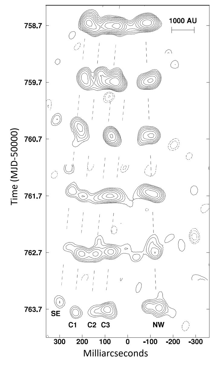
Figure 1.2: A series of 5 GHz radio images, advancing in time from top to bottom, showing a two-lobed jet of material flowing away from GRS 1915+105 (at 0 milliarcseconds) at speeds approaching $c$. Figure adapted from Fender et al., (1999).

X-ray spectral studies of LMXBs find that, in addition to a black-body like accretion disk, the systems must each contain a non-thermal ‘corona’ component. The corona is a region of non-thermal electrons somewhere in the vicinity of the compact object, and it emits X-rays via Compton upscattering. In this process, photons emitted from the disk collide with energetic electrons in the corona. The photons, on average, gain energy from these collisions and are scattered back into space; some in the direction of observers on the Earth. This leads to a characteristic power-law energy distribution signature at high energies, which can be seen in the spectra of LMXBs. As I show in the simulated LMXB energy spectrum in Figure 1.3, the emission from the corona tends to dominate above energies of $\sim 10$ keV.

Models of the geometry of the coronal region have evolved over the years. While the corona has been historically treated as if it was a single point fixed above the centre of the disk (the so-called ‘Lamp Post’ model, e.g. Różańska et al.,, 2002), more recent models tend to treat it either as an optically thin flow of material onto the compact object or equate it with the base of the radio jet (e.g. Skipper et al.,, 2013).

Figure 1.3: Two simulated, simplified spectrum of an LMXB, showing the two main components visible in X-ray: the accretion disk (blue) and the corona (orange). The disk is generally modelled as a disk black body, a sum of black bodies at different temperatures corresponding to different annuli in the disk (e.g. Mitsuda et al.,, 1984), while the corona is modeled as a power law. The left panel shows a typical spectrum of an LMXB in the high/soft state, while the right panel shows a typical spectrum of an LMXB in the low/hard state: see Section 1.2 for a discussion of accretion states. These spectra are based on spectral fits to the LMXB MXB 1658-298, performed by Sharma et al., (2018).

Another important component of an X-ray binary is the disk wind (van Paradijs et al.,, 1994). Due to the high temperatures and pressures in the inner part of the accretion disk, matter on the surface of the disk can obtain enough energy to escape the gravitational well of the compact object. This matter is ejected from the system in large-scale, high velocity winds. Studies of the spectral lines present in these winds have shown that they can have speeds approaching the speed of light (e.g. Ponti et al.,, 2012; Degenaar et al., 2014a, ).

Neutron Star X-ray Binaries

The geometry of an X-ray binary is somewhat more complicated when the compact object is a neutron star. Unlike black holes, neutron stars are in general highly-magnetised systems, and the introduction of a large, strong magnetic field to an XRB has implications for the geometry of the accretion flow. At some radius in the inner accretion disk, it is possible that the pressure exerted by this magnetic field becomes dominant over the gas and photon pressures. At this point, ionised material becomes ‘frozen-in’ to the magnetic field lines, and is only able to freely move along them. Due to the extreme temperatures present in the inner portion of the accretion disk, the vast majority of material in this region is ionised. This acts to disrupt the flow of material in the inner part of the accretion disk, and matter is funneled along field lines and onto the poles of the neutron star. This causes the poles of the neutron star to become extremely hot. As the neutron star spins, it appears to pulse as seen by an external observer due to the highly radiating magnetic poles coming in and out of view. These objects are referred to as accreting X-ray pulsars.

In addition to the effects of the magnetic field, there is another significant difference between neutron star and black hole binaries. Black holes are surrounded by an event horizon from which no light can emerge, therefore there can be no direct emission from the compact object in a black hole X-ray binary. Neutron stars on the other hand have a visible surface. As such the surface of the neutron star itself, and any phenomena that take place there, can in principle be seen.

One of the most spectacular events that can occur on the surface of a neutron star is a Type I X-ray burst (Grindlay et al.,, 1976). These occur when matter accreted onto the surface of the neutron star reaches a critical temperature and density ($\sim 2.2\times 10^{9}$ K and $3\times 10^{6}$ g cm^-3, Joss,, 1978), and nuclear fusion is triggered. This results in a flash of energy, which causes a runaway thermonuclear explosion across most or all of the neutron star surface. Type I bursts appear in data as a sudden increase in X-ray flux (1–2 orders of magnitude), followed by an power-law decay as the neutron star surface cools. As Type I bursts are distinctive features which require a surface on which to occur, they are often used as a diagnostic tool to identify an unknown compact object as a neutron star.

1.2 Low Mass X-Ray Binary Behaviour

LMXBs are not static systems, and most show variations in their luminosities over timescales of milliseconds to years. Broadly speaking, LMXBs can be divided into persistent systems and transient systems. Persistent systems have always observed to be bright since their discovery, implying a high rate of accretion at all times. In some objects, this bright, high-accretion rate state has persisted for $\geq 20$ years (e.g. GRS 1915+105, Deegan et al.,, 2009).

Transient LMXBs have a somewhat more complicated life cycle. These objects spend most of their time in a ‘quiescent’ state, during which they are faint in X-rays and only a relatively small amount of material is being accreted. However these objects also undergo ‘outbursts’, during which their luminosity increases by many orders of magnitude for a period of days to years (e.g. Frank et al.,, 1992). The frequency of these outbursts varies widely between sources, ranging from one every month or so to one every few decades or longer.

XRB outbursts tend to follow predictable evolutionary paths, evolving through a number of different ‘states’ as they progress. I show some of the states associated with black hole LMXB outbursts in Figure 1.4 on a so-called ‘hardness-intensity diagram’, which traces how the brightness and the spectral shape of a source evolve over time (see Section 3.2.3 for more information on hardness-intensity diagrams). At the start of a typical black hole LMXB outburst emission from the source is spectrally hard, i.e. dominated by higher-energy photons. This part of the outburst is referred to as a Low/Hard State (bottom-right of Figure 1.4), and a radio jet is generally visible at this time. The luminosity of the source gradually increases until it reaches some maximum, and then emission begins to become softer as the system heads towards the High/Soft State (top-right of Figure 1.4). During this transition, the system crosses the so-called ‘jet line’, and the radio jet switches off. Sources tend to spend a large portion of their outbursts in the high/soft state, appearing to meander in the hardness-intensity diagram. This meandering may include additional crossings of the jet line, causing the radio jet to flicker on and off during this period. The X-ray luminosity of the source then decreases, before the source returns to the hard state along a path of approximately constant luminosity. The source then fades back into quiescence. This typical outburst behaviour forms a distinctive ‘q’ shape in the hardness-intensity diagram, as I show in Figure 1.4, and can be thought of as the inner accretion disk filling with matter before draining onto the compact object or flowing out of the system in winds or a jet (e.g. Fender et al.,, 2004). I show typical spectra of an XRB in the low/hard and high/soft states in Figure 1.5, taken from Yamada et al., (2013).

Figure 1.4: A schematic hardness-intensity diagram adapted from Fender et al., (2004), showing the evolutionary path of a typical black hole LMXB outburst and roughly indicating the positions of quiescence (Q) and the the Low/Hard (L/H) and High/Soft (H/S) States. The jet line roughly demarcates the portion of the outburst in which a jet is observed (right of the line) from the portion in which it is not observed (left of the line).

Figure 1.5: Suzaku energy spectra of the black hole HMXB Cygnus X-1 in its low/hard (black) and high/soft (red) states, presented as typical spectra of a black hole XRB in these states. Figure taken from Yamada et al., (2013).

Neutron Star LMXBs on the other hand tend to follow one of two patterns during outburst, dividing them into so-called ‘Z sources’ and ‘atoll sources’ (e.g. van der Klis, 1989b, ). In Figure 1.6 I show examples of colour-colour diagrams (which plots two different hardness ratios against each other, see Section 3.2.3) for typical Z-type and atoll-type sources. Z sources trace out a number of ‘branches’ during outburst, each corresponding to a period of different source behaviour. Atoll sources on the other hand spend most of the time in the so-called ‘banana branch’ on the colour-colour diagram, occasionally jumping over to the ‘island state’ at larger values of hard and soft colour. Unlike black hole LMXBs which trace out their characteristic evolutionary pattern once per outburst, Z and atoll sources trace out their evolutionary paths many times per outburst. Z sources can complete the entire ‘z’ over timescales of days. Most Z sources are classified as persistent objects, although some Z sources are transient (Homan et al.,, 2007). On the other hand most atoll sources are transient, but some have been observed to be persistent (e.g. Hasinger and van der Klis,, 1989). In addition to this, at least one source is known to change between Z- and atoll-like evolutionary patterns over time (Barret and Olive,, 2002). This complex evolution over the course of each outburst highlights the fact that accretion is not a simple process, and that understanding accretion gives us better understanding of a areas of the physics of matter in extreme environments.

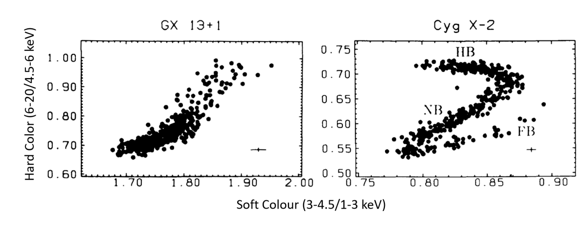
Figure 1.6: Colour-colour diagrams from van der Klis, 1989b , showing evolutionary paths of typical outbursts of Atoll-type and Z-type neutron star LMXBs (GX 13+1 and Cyg X-2 respectively). On the right-hand panel, the typical ‘branches’ of a Z-type source are marked: the High Branch (HB), Normal Branch (NB) and Flaring Branch (FB).

1.3 Relativistic Effects

One of the most obvious exotic physical environments that accretion physics sheds light on is, of course, extreme gravitational fields. General relativistic effects around compact objects are often expressed in relation to the gravitational radius $r_{g}$, defined as:

$$r_{g}=\frac{GM}{c^{2}}$$ (1.1)

Where $G$ is the gravitational constant, $c$ is the speed of light and $M$ is the mass of the compact object. $2r_{g}$ is equal to the Schwarzchild radius, or the radius of the event horizon of a non-rotating black hole with mass $M$ (Schwarzschild,, 1916).

One result of general relativity which is important when considering compact object accretion disks is the existence of an Innermost Stable Circular Orbit, or ISCO (e.g. Misner et al.,, 1973). This radius is at $6r_{g}$ from the centre of a non-rotating object, placing it well outside the event horizon of a black hole and possibly above the surface of some neutron stars. It can be shown that any non-interacting point mass crossing this boundary from the outside will continue into the black hole, whereas any point mass crossing it from the inside will continue to infinity; as such, no stable orbit can exist with a periastron smaller than this radius. It can be shown that an accretion disk is also bounded by this radius (Kozlowski et al.,, 1978), such that XRB accretion disks must all have an inner truncation radius at least this far from the compact object. Within this radius, matter falls directly onto the compact object.

A black hole can be described with 3 parameters: mass, angular momentum (or spin) and charge (Israel,, 1967). As the precursor stars to black holes are neutrally charged, it is expected that all astrophysical black holes are very close to being neutral as well. However, these precursor stars also possess non-zero angular momentum. As such, it is expected that most if not all astrophysical black holes are spinning. This spin is generally expressed as a number between 0 and 1, where 0 denotes a non-rotating black hole and 1 is the maximum permitted angular momentum the object can possess.

General relativity predicts that this spin will also have a significant effect on accretion physics. First of all, this spin changes the position of the ISCO; moving it to a maximum of $9r_{g}$ for a retrograde black hole with spin of 1 (Kerr,, 1963). A spinning black hole also distorts the space time around it, in a process known as frame-dragging (Lense and Thirring,, 1918). This forces matter close to the black hole to orbit in the same plane as it. As there is no reason to assume the outer disk orbits in the same plane as the black hole, this can lead to situations in which the accretion disk is warped, which in turn has implications for the flow of matter within it.

It is clear that general relativity should have observable implications on the flow of matter onto the accretion disk. Studying the physics of accretion therefore allows us to measure parameters such as the spin of black holes that would otherwise be inaccessible to us. Additionally, a full understanding of the accretion onto the compact objects would allow us to look for discrepancies between what is observed and what is expected from relativity. Therefore, a full understanding of accretion is one route to testing the theory of general relativity itself under some of the most extreme conditions in the universe.

Chapter 2 The Physics of Accretion

A black hole consumes matter, sucks it in, and crushes it beyond existence. When I first heard that, I thought that’s evil in its most pure.

Alice Morgan – Luther

The extreme environments in accreting systems lead to a variety of somewhat unintuitive physical effects and phenomena. In this chapter I describe a number of these effects, and delve into the history of physical and mathematical models which have been proposed to explain the effects seen in X-ray binaries.

2.1 The Shakura-Sunyaev Disk Model

To try and understand the behaviour of accretion disks, a number of authors have constructed models. Much of our understanding of the physics of astrophysical accretion disks stems from one of the earliest of these models, proposed by Nikolai Shakura and Rashid Sunyaev in 1973 (Shakura and Sunyaev,, 1973). This model specifically considered the effects of accretion onto a black hole. By showing that this would result in a system which would be bright in the X-ray, and describing how such a system would appear, this model proved pivotal in the scientific community’s acceptance of the earliest XRB identifications (e.g. Bolton,, 1972).

Shakura and Sunyaev, model the accretion disk as a structure held up by centrifugal forces, generated by the large amount of angular momentum possessed by infalling matter due to the orbit of the binary system. Frictional forces cause this angular momentum to be transferred outwards, heating up the disk and allowing matter to fall in towards the black hole. The efficiency with which this angular momentum is transferred can be thought of as a measure of the viscosity of the disk.

Shakura and Sunyaev, base their calculations on Newtonian mechanics; as such they ignore the region of the disk inwards of the ISCO at $r=3r_{g}$, where relativistic effects become important. They also assume that the disk in a steady state, that it is geometrically thin (such that height of the disk $H\ll r$ everywhere) and that it is cylindrically symmetric. The last two assumptions allow us to write down formulae for the surface density $\Sigma$, mean radial bulk velocity $u_{r}$ and accretion rate $\dot{M}$ of the disk as a functions of radius $r$:

$$\Sigma(r) = \int_{-H}^{H}\rho(r,z)dz$$ (2.1)

$$u_{r}(r) = \frac{1}{\Sigma(r)}\int_{-H}^{H}\rho(r,z)v_{r}(r,z)dz$$ (2.2)

$$\dot{M}(r) = -2\pi r\Sigma(r)u_{r}(r)$$ (2.3)

Where $\rho(r,z)$ is the density at a radius $r$ and height $z$, and $v_{r}$ is the radial velocity of the gas at this point.

Now consider the Euler equations of hydrodynamics:

$$\frac{\partial\rho}{dt}+\bm{\nabla}(\rho\bm{v}) = 0$$ (2.4)

$$\rho\left(\frac{\partial\bm{v}}{dt}+(\bm{v}\cdot\bm{\nabla})\bm{v}\right) = -\bm{\nabla}p$$ (2.5)

Where Equation 2.4 is the conservation of mass and Equation 2.5 is a differential form of Newton’s second law of motion. These equations can be cast in cylindrical co-ordinates to give 4 equations: the recast continuity equation and one motion equation for each of the radial ($r$), vertical ($z$) and azimuthal ($\theta$) directions:

$$\frac{\partial\rho}{\partial t}+\frac{1}{r}\frac{\partial(r\rho v_{r})}{\partial r}+\frac{1}{r}\frac{\partial v_{\theta}}{\partial\theta}+\frac{\partial v_{z}}{\partial z} = 0$$ (2.6)

$$\rho\left(\frac{\partial v_{r}}{\partial t}+v_{r}\frac{\partial v_{r}}{\partial r}+\frac{v_{\theta}}{r}\frac{\partial v_{r}}{\partial\theta}+v_{z}\frac{\partial v_{r}}{\partial z}-\frac{v_{\theta}^{2}}{r}\right) = \frac{-\partial p}{\partial r}$$ (2.7)

$$\rho\left(\frac{\partial v_{\theta}}{\partial t}+v_{r}\frac{\partial v_{\theta}}{\partial r}+\frac{v_{\theta}}{r}\frac{\partial v_{\theta}}{\partial\theta}+v_{z}\frac{\partial v_{\theta}}{\partial z}+\frac{v_{r}v_{\theta}}{r}\right) = \frac{-\partial p}{\partial\theta}$$ (2.8)

$$\rho\left(\frac{\partial v_{z}}{\partial t}+v_{r}\frac{\partial v_{z}}{\partial r}+\frac{v_{\theta}}{r}\frac{\partial v_{z}}{\partial\theta}+v_{z}\frac{\partial v_{z}}{\partial z}\right) = \frac{-\partial p}{\partial z}$$ (2.9)

By assuming that the disk is in a steady state and cylindrically symmetric, we can set all $\frac{\partial}{\partial\theta}$ and $\frac{\partial}{\partial t}$ terms to zero, simplifying equations 2.7 to 2.9:

$$\rho\left(v_{r}\frac{\partial v_{r}}{\partial r}+v_{z}\frac{\partial v_{r}}{\partial z}-\frac{v_{\theta}^{2}}{r}\right) = \frac{-\partial p}{\partial r}$$ (2.10)

$$\rho\left(v_{r}\frac{\partial v_{\theta}}{\partial r}+v_{z}\frac{\partial v_{\theta}}{\partial z}+\frac{v_{r}v_{\theta}}{r}\right) = 0$$ (2.11)

$$\rho\left(v_{r}\frac{\partial v_{z}}{\partial r}+v_{z}\frac{\partial v_{z}}{\partial z}\right) = \frac{-\partial p}{\partial z}$$ (2.12)

We can average the density term on left-hand side of Equation 2.6 in the $z$-direction, and substitute in the results from Equations 2.1 to 2.3 to find:

$$\frac{1}{r}\frac{d}{dr}\left(r\int_{-H}^{H}\rho v_{r}dz\right) = 0$$ (2.13)

$$\frac{1}{r}\frac{d(r\Sigma u_{r})}{dr} = 0$$ (2.14)

$$\frac{-1}{2\pi r}\frac{d\dot{M}}{dr} = 0$$ (2.15)

Therefore the rate of inwards matter flow $\dot{M}$, or the accretion rate, is constant at all $r$.

Using the fact that the angular velocity $\omega$ of an element in the gas can be written as $\omega=v_{\theta}/r$, we can re-write Equation 2.10 as:

$$\rho\left(v_{r}\frac{\partial v_{r}}{\partial r}-\omega^{2}r\right)=-\frac{\partial p}{\partial r}-\rho v_{z}\frac{GM}{r^{2}}$$ (2.16)

Where the term $\frac{GM}{r^{2}}$ has been introduced to account for the fact that the gradient of the gravitational field in the $r$ direction is non-zero. This leads to:

$$\rho\left(v_{r}\frac{\partial v_{r}}{\partial r}-\omega^{2}r\right)=-\frac{\partial p}{\partial r}-\rho\omega_{k}^{2}r$$ (2.17)

Assuming that is thin and angular momentum is only transferred slowly, i.e. $v_{r}\frac{\partial v_{r}}{\partial r}\ll\omega$, this leads to:

$$\omega\approx\omega_{k}$$ (2.18)

Showing that gas elements in the disk orbit at Keplerian speeds.

Using similar logic, Equation 2.12 becomes:

$$\rho\omega_{k}^{2}z=\frac{-\partial p}{\partial z}$$ (2.19)

The ideal gas law $p=\rho RT$ can then be used to rewrite equation 2.19:

$$\frac{p}{RT}\omega_{k}^{2}z=\frac{-\partial p}{\partial z}$$ (2.20)

If we assume that the disk is chemically homogeneous and isothermal in the $z$-direction, then neither $R$ nor $T$ depend on $z$. Equation 2.20 then admits the solution:

$$\rho=\rho_{0}(r)e^{\left(\frac{-z^{2}\omega_{k}^{2}}{2RT}\right)}=\rho_{0}(r)e^{\frac{-z^{2}}{2H_{s}^{2}}}$$ (2.21)

Where $\rho_{0}$ is the density at radius $r$ when $z=0$. As such, the density of the disk has a Gaussian profile in the $z$-direction, with a scale-width $H_{s}$ given by:

$$H_{s}=\frac{\sqrt{RT}}{\omega_{k}}$$ (2.22)

This shows that the scale height of the disk is finite for all $r$. As the integral between $-\infty$ and $+\infty$ of a Gaussian with a finite scale-width is finite, the disk contains a finite amount of matter.

Finally, Shakura and Sunyaev, looked at the solutions to Equation 2.11. As every term in this equation depends on either $v_{\theta}$ or a derivative thereof, this equation admits the solutions $\rho=0$ or $v_{\theta}=0$. Both of these solutions imply accretion rates of zero, as any matter in the disk must have a non-zero density and angular momentum. In order to resolve this problem, Shakura and Sunyaev, (1973) add the divergence of the viscous stress tensor (Landau and Lifshitz,, 1959) to the right-hand side of Equation 2.11 to represent the effects of viscosity within the disk. By doing this, they find the following two results:

$$\dot{M} = \frac{4\pi H_{s}\eta_{b}r}{\omega}\frac{\partial\omega}{\partial r}$$ (2.23)

$$\dot{M} = 6\pi\eta_{b}H_{s}$$ (2.24)

Equation 2.23 confirms that the disk is a differential rotator, while Equation 2.24 confirms that accretion can only take place when $\eta_{b}$ (the bulk viscocity) is non-zero.

Shakura and Sunyaev, (1973) found that molecular viscosity alone cannot be high enough to result in the high values of $\dot{M}$ inferred for observed XRBs. Instead, the authors assume that turbulence is present in the disk. Using formulae pertaining to turbulent hydrodynamics, and by ignoring supersonic perturbations, they find an upper bound on bulk viscosity $\eta$:

$$\eta_{b}\leq\frac{2}{3}\rho_{0}H\sqrt{RT}$$ (2.25)

As such, they define a dimensionless viscosity parameter $\alpha$ as:

$$\alpha\equiv\frac{3\eta_{b}}{2\rho_{0}H\sqrt{RT}}\quad\quad\quad 0<\alpha\leq 1$$ (2.26)

2.1.1 The source of Turbulence

Shakura and Sunyaev, (1973) do not answer the question of what physical process causes the turbulence required to stabilise accretion disks. Balbus and Hawley, (1991) were among the first to propose the Magnetorotational Instability (MRI, Velikhov,, 1959; Chandrasekhar,, 1961) as the source of this turbulence. MRI is a process which occurs in an ionised and differentially rotating disk. Fluctuations in the material in the disk generate internal magnetic fields. The field lines associated with these fields, in general, extend a finite distance in the radial direction, thus connecting gas elements at different radii. As gas elements in a Shakura-Sunyaev accretion disk orbit the compact object at Keplerian speeds, elements of gas at different radii move at different orbital speeds. As such, these internal magnetic field lines become stretched as gas orbits the compact object. This field line stretching imparts a torque on the gas elements, causing the outer, slower element to speed up and the inner, faster element to slow down. As such, the net result of this process is an outwards transfer of angular momentum.

Balbus and Hawley, (1991) found that the angular momentum transfer due to MRI was more significant than that due to friction, hydrodynamic turbulence or other sources in an accretion disk. They suggest therefore that MRI is the main component of outwards angular momentum transfer, and thus of $\alpha$, in astrophysical accretion disks.

2.2 Accretion Phenomena

The extreme physics involved in accretion onto compact objects leads to a number of non-intuitive physical phenomena. In this section I describe a number of these theoretical effects, and explain how these phenomena manifest in physical LMXBs.

2.2.1 The Eddington Limit

Consider an element of gas at distance $r$ from a compact object, with mass $m$. This element of gas is acted on by a inwards-pointing gravitational force given by:

$$F_{G}=\frac{GMm}{r^{2}}$$ (2.27)

Where $M$ is the mass of the compact object.

If we assume that a luminosity $L$ is emitted isotropically from the compact object, then the electromagnetic flux at distance $r$ is given by:

$$\phi(r)=\frac{L}{4\pi r^{2}}$$ (2.28)

Electromagnetic radiation exerts a pressure on material corresponding to $\phi/c$. As such, the radiation from the X-ray binary exerts an outwards force on our gas element corresponding to:

$$F_{L}=\frac{\kappa m\phi(r)}{c}=\frac{L\kappa m}{4\pi r^{2}c}$$ (2.29)

Where $\kappa$ is the opacity of the cloud, or its surface area per unit mass.

If $F_{G}$ and $F_{L}$ are equal, then no net force is exerted on our cloud of matter and it will not accrete onto the compact object. This happens when:

$$F_{G} = F_{L}$$ (2.30)

$$\frac{GMm}{r^{2}} = \frac{L\kappa m}{4\pi r^{2}c}$$ (2.31)

$$L = \frac{GMm}{r^{2}}\frac{4\pi r^{2}c}{\kappa m}$$ (2.32)

$$L = \frac{4\pi GMc}{\kappa}$$ (2.33)

This luminosity, denoted as $L_{E}$, is the Eddington luminosity; the theoretical maximum isotropic luminosity an object can emit and still have spherically symmetric accretion take place. It only depends on the mass of the compact object $M$ and the opacity of the accreting material $\kappa$, which in turn depends on the chemical composition of the accretion disk. As accretion disks tend to be dominated by ionised hydrogen, $\kappa$ is usually assumed to be $\sigma_{T}/m_{p}$, where $\sigma_{T}$ is the Thomson scattering cross-section of an electron and $m_{p}$ is the mass of a proton. This assumption yields the final formula which only depends on the mass of the compact object:

$$L_{E}=\frac{4\pi GMm_{p}c}{\sigma_{T}}$$ (2.34)

The luminosity due to matter falling into a compact object can be expressed as:

$$L=\eta\dot{M}c^{2}$$ (2.35)

Where $\dot{M}$ is the accretion rate and $\eta$ is the efficiency at which the gravitational potential energy of infalling matter is converted to outgoing radiation. As such, $L_{E}$ also corresponds to a limiting accretion rate $\dot{M}_{E}$.

However, a number of X-ray binaries have been seen to shine at luminosities far above this limit; in one of the most extreme cases, the confirmed neutron star XRB M82 X-1 has a luminosity of $\sim 100L_{E}$ (Bachetti et al.,, 2014). This super-Eddington accretion is possible due to the fact that a number of assumptions made when calculating the Eddington limit do not apply to physical XRBs. In particular, the calculation performed above assumes that both accretion on to the compact object, as well as electromagnetic emission from it, are isotropic. An object may exceed the Eddington Limit if it is accreting anisotropically, as is the case for XRBs as these systems accrete from near-planar disks. In this case the assumptions behind the calculation of the Eddington Limit break down, and more radiation can be emitted away from the plane of the disk, decreasing the radiation pressure on infalling material. Anisotropically emitting systems may appear to further exceed the Eddington limit via beaming effects. An XRB beaming its radiation in the direction of the Earth would lead us to infer an artificially high value of $L$, and thus overestimate its luminosity with respect to the Eddington Limit.

Despite these setbacks, the Eddington Luminosity is a useful tool to compare XRBs with different compact object masses. By expressing the luminosity of an object as a fraction of its Eddington Limit, objects can be rescaled in such a way that we can compare how dominant radiation pressure must be in each accretion disk.

2.2.2 The Propeller Effect

Another limit on accretion rate arises when one considers the effect of a strong neutron star magnetic field. To understand this effect, we must first define two characteristic radii of such a system.

First, assume that the magnetic field of the neutron star can be approximated as a set of rigid field lines which are anchored to points on the neutron star surface. The magnetic field can then be thought of as a ‘cage’ which rotates with the neutron star at its centre. The straight-line speed of a point on this rotating cage is given by:

$$v_{\nu}(r)=2\pi r\nu$$ (2.36)

Where $r$ is the distance from the neutron star centre and $\nu$ is the rotation frequency of the neutron star. This can be compared with the Keplerian speed, or the speed of a particle in a Keplerian orbit around the compact object. This is given by:

$$v_{K}(r)=\sqrt{\frac{GM}{r}}$$ (2.37)

Where $M$ is the mass of the neutron star. By setting these equal, we can find the radius at which the magnetic field is rotating at the same speed as a particle in a Keplerian orbit:

$$v_{\nu}(r) = v_{K}(r)$$ (2.38)

$$2\pi r\nu = \sqrt{\frac{GM}{r}}$$ (2.39)

$$r^{3} = \frac{GM}{4\pi^{2}\nu^{2}}$$ (2.40)

$$r = \sqrt[3]{\frac{GM}{4\pi^{2}\nu^{2}}}$$ (2.41)

This radius is denoted as $r_{c}$, the co-rotation radius. Inside of this radius, a particle in an equatorial Keplerian orbit has a greater velocity than the magnetic field lines; outside this radius, the magnetic field lines are moving faster. To understand the significance of this radius, we must define another characteristic radius of the system.

In a neutron star accretion disk, there are three significant sources of pressure: gas (or ram) pressure $P_{g}$, radiation pressure $P_{\gamma}$ and magnetic pressure $P_{\mu}$. Whichever pressure is dominant in a given location will govern the physics of matter in that region.

Photon pressure falls off sharply outwards from the inner disk, so it can be assumed to be negligible in the region of the disk considered here. We can then calculate where in the disk each of the remaining two pressures dominates.

Assuming that the neutron star behaves as a magnetic dipole, the magnetic pressure at a point a distance $r$ above its equator can be given as:

$$P_{\mu} = \frac{B^{2}}{2\mu_{0}}$$ (2.42)

$$B(r) = B_{0}\left(\frac{R_{NS}}{r}\right)^{3}$$ (2.43)

$$\therefore\quad P_{\mu} = \frac{B_{0}^{2}}{2\mu_{0}}\left(\frac{R_{NS}}{r}\right)^{6}$$ (2.44)

Where $\mu_{0}$ is the vacuum permeability, $B_{0}$ is the equatorial magnetic field strength at the neutron star surface, $R_{NS}$ is the radius of the neutron star and Equation 2.43 is the equation for the magnetic field strength above the equator of a dipole.

The functional form of the ram pressure depends on the assumed accretion geometry of the system. As when calculating the Eddington Limit, one can assume the simplest possible case of spherically accreting free-falling matter. The ram pressure is then given by:

$$P_{g}=\frac{\dot{M}}{4\pi r^{2}}\sqrt{\frac{2GM}{r}}$$ (2.45)

When $P_{\mu}>P_{g}$, accreting material is dominated by magnetic pressure in such a way that material is ‘frozen’ onto magnetic field lines (Alfvén,, 1942); this results in material flowing onto the neutron star surface along magnetic field lines onto the poles, as described in section 1.1.2. It is possible to express the region of the accretion disk within which matter is magnetically dominated:

$$P_{g} < P_{\mu}$$ (2.46)

$$\frac{\dot{M}}{4\pi r^{2}}\sqrt{\frac{2GM}{r}} < \frac{B_{0}^{2}}{2\mu_{0}}\left(\frac{R_{NS}}{r}\right)^{6}$$ (2.47)

$$\frac{GM\dot{M}^{2}}{8\pi^{2}r^{5}} < \frac{B_{0}^{4}}{4\mu_{0}^{2}}\left(\frac{R_{NS}}{r}\right)^{12}$$ (2.48)

$$r^{7} < \frac{2\pi^{2}}{G\mu_{0}^{2}}\frac{B_{0}^{4}R_{NS}^{12}}{M\dot{M}^{2}}$$ (2.49)

$$r < \sqrt[7]{\frac{2\pi^{2}}{G\mu_{0}^{2}}\frac{B_{0}^{4}R_{NS}^{12}}{M\dot{M}^{2}}}$$ (2.50)

The critical radius, the magnetospheric or Alfvén radius, is denoted as $r_{\mu}$.

Now it is possible to consider what happens to matter approaching $r_{\mu}$ in two different physical regimes. First of all, consider a system in which the corotation radius $r_{c}>r_{\mu}$. In this case, which we show diagrammatically in panel A of Figure 2.1, magnetic field lines at $r_{\mu}$ are moving slower than the Keplerian speed. An element of matter approaching this radius from a Keplerian orbit will experience a torque slowing it down as it freezes onto the field lines. This decrease in orbital speed causes the element’s altitude above the neutron star surface to decrease. This in turn pulls the element further into the magnetically-dominated regime and allows it to accrete freely along the field line onto the neutron star.

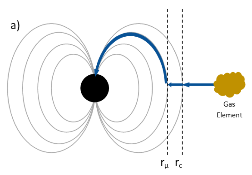
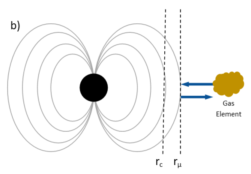
Figure 2.1: Diagrams showing the path of an element of gas in a neutron star accretion disk for different arrangements of the corotation ($r_{c}$) and magnetospheric ($r_{\mu}$) radii. In panel a), the gas falls freely inwards until it reaches $r_{\mu}$, at which point it freezes onto a magnetic field line. As $r_{\mu}<r_{c}$, the magnetic field lines (grey lines) are rotating more slowly than the gas element at this point. As such, the gas element experiences torque which slows it down, decreasing its altitude above the neutron star surface (black circle) and causing it to accrete along the magnetic field line. In panel b), $r_{\mu}<r_{c}$. As such, the magnetic field lines are rotating faster than the gas element at $r_{\mu}$. The gas element experiences a torque which speeds it up at this point, increasing its altitude and preventing it from accreting onto the neutron star.

Now we can consider what happens when $r_{c}<r_{\mu}$. In this case, which we show diagrammatically in panel B of Figure 2.1, field lines at $r_{\mu}$ are moving faster than the Keplerian speed. An element of matter approaching $r_{\mu}$ will therefore experience a torque speeding it up as it becomes frozen onto magnetic field lines. This will increase its altitude, driving it back away from $r_{\mu}$. In this case, the magnetospheric radius acts as a barrier to infalling matter, repelling any gas that approaches it and stopping accretion onto the neutron star surface. This set of circumstances is known as the ‘propeller regime’, due to the rapidly rotating field lines acting like a ‘propeller’ which blows the inner part of the disk away.

As the propeller regime is expected to occur only for $r_{c}<r_{\mu}$, it is possible to work out what kind of system this should be observed in:

$$r_{c} < r_{\mu}$$ (2.51)

$$\left(\frac{GM}{4\pi^{2}\nu^{2}}\right)^{1/3} < \left(\frac{2\pi^{2}}{G\mu_{0}^{2}}\frac{B_{0}^{4}R_{NS}^{12}}{M\dot{M}^{2}}\right)^{1/7}$$ (2.52)

$$M^{10/21}\dot{M}^{2/7} < k\nu^{2/3}B_{0}^{4/7}R_{NS}^{12/7}$$ (2.53)

Where $k$ is a constant. Assuming that the radius and mass of neutron stars does not vary much, this inequality tells us that the propeller regime is more likely to be observed in neutron star XRBs with a high spin frequency and a high magnetic field. The inequality shown in 2.53 also tells us that the propeller effect places a lower limit on accretion in such systems: accretion is not possible unless infalling matter can apply enough ram pressure to push the magnetospheric radius inside the corotation radius.

There are numerous problems with this relatively simplistic view of accretion in a highly magnetic regime. Much like the formulation of the Eddington Limit I present in Section 2.2.1, the above formulation of the propeller effect depends on an unphysical spherical accretion geometry. It also includes the assumption that the magnetic field lines can in no way be warped by the movement of ionised matter on them.

White and Stella, (1988) have shown that, in neutron stars, the magnetospheric radius may be close enough to the compact object that photon pressure cannot be safely neglected. White and Stella, find two different possible behaviours of the magnetospheric radius in such a regime, depending on how $\alpha$ varies with $r$ and how the disk reacts to the magnetic field. For a perfectly diamagnetic disk, they show that the magnetospheric radius should not depend on the accretion rate, preventing the formation of a propeller regime entirely. For a case in which gas pressure is the dominant contributor to viscous stress, they find that the magnetospheric radius is up to $\sim 30$ times smaller than that calculated by equation 2.50. Additionally, Ertan, (2017) has analytically shown that an optically thick accretion disk can only be in a stable propeller regime when the inner disk radius is $\gtrsim 15$ times smaller that the $r_{\mu}$ naïvely calculated in equation 2.50. This in turn results in a several orders of magnitude reduction in the critical accretion rate at the onset of the propeller regime in a given system, raising questions as to whether the effect would be observable at such low luminosities.

Despite these difficulties, an effect observationally similar to the propeller effect is observed in a number of astrophysical neutron star XRBs (e.g. the cessation of pulsed emission while the source is still in outburst and the neutron star is actively spinning up or down, Fabian,, 1975; Fürst et al.,, 2017) and other systems (e.g. the observation of a sudden steepening in lightcurves during the decays of outbursts, interpreted by e.g. Campana et al.,, 2017 as the onset of the propeller phase). Therefore it is likely that a propeller effect in some form is likely able to explain what we see in nature.

2.2.3 Disk Instabilities

A number of effects can cause an accretion disk, or portions of it, to become unstable. Some of these instabilities can set up limit cycles of behaviour in the disk, resulting in quasi-periodic fluctuations in the object’s intensity or colour as seen from Earth. I describe a number of these instabilities here.

One of the first such instabilities to be described was discovered by Lightman and Eardley, (1974). Using the assumptions present in the thin disk models of Shakura and Sunyaev, (1973) and Novikov and Thorne, (1973), Lightman and Eardley, calculate the diffusion of the gas in such a disk. They show that the diffusion coefficient in the radial direction of radiatively dominated disk is negative. As such, any initially smooth disk under these conditions tends to separate into thin, dense annuli. As such any sufficiently thin disk, with $\alpha$ consistent with the prescription of Shakura and Sunyaev, (1973) is unstable.

Shakura and Sunyaev, (1976) described another instability which takes place in the radiation pressure-dominated region near the inner edge of accretion disks. They find that steady state accretion in such a regime is only possible for a single value of $\alpha$, and hence this region is unstable under small perturbations of viscosity. They argue that an instability due to this effect may take the form of propagating wavefronts in the inner disk, which in turn may cause some of the quasiperiodic fluctuations which are observed in these objects.

A further disk instability arises by considering the propeller effect (see Section 2.2.2), and specifically considering neutron star LMXBs in which the magnetopsheric radius and co-rotation radius are similar ($r_{c}\approx r_{\mu}$, e.g. Spruit and Taam,, 1993). At this boundary, a small increase in global accretion rate from the donor star pushes $r_{\mu}$ inwards such that $r_{\mu}<r_{c}$. In this regime, the neutron star accretes freely, and the system is relatively bright in X-rays. However, a slight decrease in global accretion rate causes $r_{\mu}<r_{c}$: in this regime, accretion onto the compact object’s surface is halted and the system is relatively faint in X-rays. This effect causes a small fluctuation in accretion rate to convert to a large fluctuation in luminosity between two quasi-stable values. This effect is believed to be behind the so-called ‘hiccup accretion’ seen in X-ray binaries such as IGR J18245-2452 (Ferrigno et al.,, 2014) and 1RXS J154439.4-112820 (Bogdanov and Halpern,, 2015).

2.3 GRS 1915+105 and IGR J17091-3624

One famous system in which disk instabilities are extremely apparent is the black hole LMXB GRS 1915+105. GRS 1915+105 (Castro-Tirado et al.,, 1992), hereafter GRS 1915, is a black hole LMXB which accretes at between a few tens and more than 100% of its Eddington Limit (e.g. Vilhu,, 1999; Done et al.,, 2004; Fender and Belloni,, 2004). The system lies at a distance of $8.6\pm 2.0$ kpc (Reid et al.,, 2014), and consists of a 12.4$\pm$2.0 M_⊙ black hole and a $<1$ M_⊙ K-class giant companion star (Reid et al.,, 2014; Ziółkowski and Zdziarski,, 2017).

The components of GRS 1915 have the longest known orbital period of any LMXB (Greiner et al.,, 2001), in turn implying that this system has the greatest orbital separation and the largest accretion disk. GRS 1915 has been in outburst since its discovery in 1992 (Castro-Tirado et al.,, 1992), and the extreme length of this ongoing outburst is believed to be related to the large size of its accretion disk.

GRS 1915 is also notable for the incredible variety and complexity of behaviours it exhibits over timescales of seconds to minutes (e.g. Yadav et al.,, 2000; Belloni et al.,, 2000). In total, at least 15 distinct ‘variability classes’ have been described (Belloni et al.,, 2000; Klein-Wolt et al.,, 2002; Hannikainen et al.,, 2007; Pahari and Pal,, 2009), a number of which I show lightcurves of in Figure 2.2. The system tends to stay in one variability class for no more than a few days but similar patterns are often repeated many months or years later, suggesting some capacity of the system to ‘remember’ which variability classes it can show.

Figure 2.2: Typical lightcurves of a selection of variability classes seen in GRS 1915, taken by the PCA instrument aboard RXTE. The classes are labelled according to the Greek letter names assigned to them in Belloni et al., (2000).

The variability classes of GRS 1915 consist of repeating patterns of flares, dips and periods of noisy fluctuation, with a range of amplitudes and timescales. The behaviour of the source during these classes, which are usually denoted by the Greek letter names assigned to them by Belloni et al., (2000), can range from highly quasi-periodic to apparently entirely unstructured. The $\rho$ class, also referred to as the ‘heartbeat’ class due to the similarity of its lightcurve to the output of an electrocardiagram, consists of sharp quasiperiodic flares with a recurrence time of a few tens of seconds (Middle-right panel of Figure 2.2). Other classes, such as class $\kappa$ shown in the top-left panel of Figure 2.2, consist of quasiperiodic fluctuations between two quasistable count rates: in the case of class $\kappa$, there is also a period of highly structured sub-second variability at each transition between these two classes. Finally, two classes ($\chi$ and $\phi$, an example of the latter is shown in the bottom-right panel of Figure 2.2) show no significant variability other than red noise; these classes are separated from each other based on their spectral properties. It has been suggested they they may be equivalent to the hard state seen in other outbursting LMXBs (van Oers et al.,, 2010), providing a possible link between the behaviour of GRS 1915 and the behaviour of more typical LMXBs.

The dramatic variability seen in GRS 1915 was long thought to be unique, driven by its unusually high accretion rate (e.g. Belloni et al., 1997b, ). However in 2011, Altamirano et al., 2011b unambiguously identified GRS 1915-like variability in a second object: the black hole LMXB IGR J17091-3624 (hereafter IGR J17091). This object is much fainter than GRS 1915: Altamirano et al., 2011b showed that, assuming that this object accretes at its Eddington Limit by analogy with GRS 1915, the object may either be out in the halo of the Galaxy (at $\gtrsim 20$ kpc) or harbour the smallest mass black hole known to science ($\lesssim 3$ M_⊙). The companion star to the black hole in this system has not been definitively identified (Chaty et al.,, 2008).

Much like GRS 1915, IGR J17091 displays a number of distinct classes of variability over time, and a number of these have been identified as being similar to the classes seen in GRS 1915 (e.g. Altamirano et al., 2011b, ; Zhang et al.,, 2014). Unlike GRS 1915, IGR J17091 displays the pattern of outbursts and quiescence more commonly seen in LMXBs; known outbursts of IGR J17091 occurred in 2011 and 2016, and GRS 1915-like variability was observed in both (Reynolds et al.,, 2016).

There are a number of notable differences between variability classes in GRS 1915 and IGR J17091. In general, variability classes in IGR J17091 occur over shorter timescales than their counterparts in GRS 1915. In addition to this, hard emission tends to lag soft emission in the variability classes of GRS 1915 (e.g. Janiuk and Czerny,, 2005), while the opposite trend has been found in the ‘heartbeat’-like class of IGR J17091 (Altamirano et al., 2011b, ).

In addition to GRS 1915 and IGR J17091, there have been claims that a third LMXB displays GRS 1915-like variability. Bagnoli and in’t Zand, (2015) report on two observations of MXB 1730-335, also known as the ‘Rapid Burster’, which show lightcurve patterns remarkably similar to those seen in the $\rho$ and $\theta$ classes of GRS 1915. The presence of GRS 1915-like variability in the Rapid Burster is significant for a number of reasons: unlike GRS 1915 or IGR J17091, the Rapid Burster is known to contain a neutron star accreting at no more than 20% of its Eddington Limit, thereby ruling out any black hole-specific or near-Eddington-specific explanations for this behaviour. In addition to this, the Rapid Burster is one of only 2 objects known to undergo so-called Type II X-Ray bursts (see Section 2.4), suggesting a possible link between these two phenomena. However, as it has only been observed twice in the $\sim 30$ years since the object was discovered, the true nature of the apparent GRS 1915-like variability in the Rapid Burster remains unclear.

2.3.1 A History of Models of GRS 1915-like Variability

Over the years, a number of models and physical scenarios have been suggested to explain the complex variability seen in GRS 1915-like systems. Successful models must also be able to explain why this type of variability is not seen in a wider array of sources.

One of the most best-studied classes of GRS 1915-like variability is Class $\rho$, the ‘heartbeat’ class. This variability class is present in both GRS 1915 and IGR J17091 (e.g. Altamirano et al., 2011b, ), and has been the focus of many of the models proposed to explain GRS 1915-like variability. It has been shown that hard X-ray photons lag soft X-ray photons in this class (e.g. Janiuk and Czerny,, 2005; Massaro et al.,, 2010), suggesting that hard emission from this source is somehow caused by the softer emission. Other classes in GRS 1915 which show quasi-periodic flaring behaviour also exhibit this phase lag. Previous authors have established models to explain both the hard photon lag as well as the ‘heartbeat’-like flaring itself, generally based on the instability in a radiation-dominated disk first formulated by Shakura and Sunyaev, (1976) (see Section 2.2.3).

Belloni et al., 1997a first proposed an empirical model for flaring in GRS 1915. They suggested that this behaviour is due to a rapid emptying of a portion of the inner accretion disk, followed by a slower refilling of this region over a viscous timescale. Belloni et al., 1997a divided data from a given observation into equal-sized 2-Dimensional bins in count rate-colour space. A spectral model was then fit to each of these bins independently to perform ‘pseudo’-phase-resolved spectroscopy (compare with the method outlined in Section 3.2.3). They showed that the time between flaring events correlates with the maximum inner disk radius during the flare; i.e., a correlation between the amount of the disk which is emptied and the time needed to refill it. They go on to suggest that their model is able to explain all flaring-type events seen in GRS 1915.

The scenario proposed by Belloni et al., 1997a was mathematically formalised by Nayakshin et al., (2000), who found that it was not consistent with a ‘slim’ accretion disk (Abramowicz et al.,, 1988) or with a disk in which viscosity $\alpha$ is constant with respect to radius. As such, their model consists of a cold accretion disk with a modified viscosity law, a non-thermal electron corona and a transient jet of discrete plasma emissions which are ejected when the bolometric luminosity approaches the Eddington Limit. Using their model, Nayakshin et al., (2000) found that some formulations of $\alpha(r)$ result in the disk oscillating between two quasi-stable branches in viscosity-temperature space, over timescales consistent with those seen in the flaring of GRS 1915; they found that this occurs for accretion rates greater than 26% of the Eddington limit. They also found that by varying the functional form of $\alpha(r)$, their model gives rise to a number of lightcurve morphologies which generally match what is seen in data from GRS 1915. Janiuk et al., (2000) built on this model further by including the effect of the transient jet in cooling the disk; an effect not considered in the model by Nayakshin et al., (2000). In this formulation, Janiuk et al., (2000) found that GRS 1915-like variability should occur at luminosities as low as 16% of Eddington. The criteria of a relatively low accretion rate in these models suggests that many more black hole LMXBs should show GRS 1915-like behaviour, which is at odds with observations. Additionally, they are unable to explain GRS 1915-like behaviour in objects with even lower accretion rates, such as the $\rho$-like behaviour reported by Bagnoli and in’t Zand, (2015) in the Rapid Burster.

Belloni et al., (2000) found that variability in GRS 1915 can be empirically described by transitions between three phenomenological states, which differ in luminosity and hardness ratio:

1. State B: high rate, high 5–13/2–5 keV hardness ratio.

2. State C: low rate, low 5–13/2–5 keV hardness ratio, variable 13–60/2–5 keV hardness ratio.

3. State A: low rate, low 5–13/2–5 keV hardness ratio, lowest 13–60/2–5 keV hardness ratio.

Belloni et al., find that no variability class shows a transition from state C to state B, and they suggest that this transition is forbidden. The phenomenological scenario they establish is at odds with the model of Nayakshin et al., (2000), which only results in two quasi-stable states; one high rate and one low rate state.

Nobili, (2003) tried to account for the hard X-Ray lag by considering a scenario in which a significant proportion of the X-Ray disk variability comes from a single hotspot. They suggest that the lag corresponds to a light travel time, after which a portion of this emission is Comptonised by the jet. In this case, the geometric location of this hotspot determines the magnitude of this lag. This scenario goes some way to explaining why GRS 1915 is special, as it requires the presence of a jet during a soft-like state.

Tagger et al., (2004) propose a magnetic explanation for the ejection of the inner accretion disk required by Nayakshin et al., (2000) and Janiuk et al., (2000). In their scenario, they suggest the existence of a limit cycle in which a poloidal magnetic field is advected towards the inner disk during the refilling of this region. Associated field lines are then destroyed in reconnection events, releasing energy which results in the expulsion of matter from the inner disk. They suggest that the three quasi-stable states proposed by Belloni et al.,, 2000 can be explained as states in the inner accretion disk with different values of plasma $\beta$.

Janiuk and Czerny,, 2005 attempt to explain the hard lag in the heartbeats of GRS 1915 more simply, by proposing a model in which it is caused by the non-thermal corona smoothly adjusting to changes in luminosity from the disk. They base the variability of the disk on the model of Nayakshin et al.,, 2000, and show that the presence of a non-thermal corona which reacts to this variability naturally reproduces the lag behaviour seen in Class $\rho$ in GRS 1915.

Merloni and Nayakshin,, 2006 also propose a magnetic explanation for the reformulation of $\alpha(r)$ required by the model of Nayakshin et al.,, 2000. Assuming that the viscosity in the accretion disk is dominated by turbulence due to the magnetorotational instability, they find that allowing for a magnetically dominated corona naturally allows for the forms of $\alpha(r)$ required by Nayakshin et al.,, 2000.

Zheng et al.,, 2011 propose a model which suggests that, when the effects of a magnetic field are included, the accretion rate threshold for GRS 1915-like variability should be $\sim 50$% of Eddington; significantly higher than the 16% or 26% reported by Janiuk et al.,, 2000 or Nayakshin et al.,, 2000. Zheng et al., go on to suggest that this type of variability is only seen in GRS 1915 due to this source having the highest accretion rate of all permanently soft-state sources. As such, this scenario still relies on a high accretion rate to trigger GRS 1915-like variability, but it is more consistent with observations than the models of Janiuk et al.,, 2000 or Nayakshin et al.,, 2000.

Neilsen et al.,, 2011 performed phase-resolved spectroscopy of the $\rho$ class in GRS 1915. They find a hard ‘spike’ after each flare, which they associate with the hard lag in this class previously noted by e.g. Janiuk and Czerny,, 2005. They propose a scenario in which high-velocity winds formed by the ejection of matter from the inner disk interact directly with the corona after a light travel time. The corona then re-releases this energy as a hard bremsstrahlung pulse, causing the hard count rate spike seen in phase-resolved spectra. This scenario is outlined in Figure 2.3. The authors expand on this scenario in Neilsen et al.,, 2012 to suggest that this mechanism can explain all classes in GRS 1915 which display $\rho$-like flaring. However, this scenario still relies on the model of Nayakshin et al.,, 2000 to generate the instability in the disk, and it implies that hard photons should always lag soft photons in heartbeat-like variability classes. Significantly, this scenario is therefore unable to explain the soft lags which have been observed in $\rho$-like variability in IGR J17091 (Altamirano et al., 2011b, ).

Figure 2.3: A schematic diagram illustrating the the process described by Neilsen et al.,, 2011 to describe the $\rho$ variability class in GRS 1915+105. 1) The X-ray emission from the system originates from both the accretion disk truncated at an inner radius $r_{in}$ (grey) and a corona of non-thermal electrons (white ellipse). At some time $t$, an overdensity in the accretion disk (formed by the instability described by Shakura and Sunyaev,, 1976) propagates inwards towards $r_{in}$. 2) As the inner disc heats up, $r_{in}$ begins to slowly increase due to an increase in photon pressure. This destabilises the disc. 3) At some critical density, the disc becomes too unstable and collapses inwards, greatly decreasing $r_{in}$ and raising the inner disc temperature. 4) The sudden increase in emission exceeds the local Eddington limit at $r_{in}$, ejecting matter from the inner accretion disc in the form of extreme winds. 5) Having been excited by matter in the winds passing through it, the non-thermal electron cloud emits a hard Brehmsstrahlung ‘pulse’.

Neilsen et al.,, 2011 also perform phase-resolved spectroscopy (see Section 3.2.3) of the flaring during $\rho$ variability. In their fitting, Neilsen et al.,, 2011 consider three spectral models:

1. An absorbed disk black body with a high energy cutoff, of which some fraction has been Compton upscattered

2. An absorbed disk black body with a high energy cutoff, plus a Compton component with a seed photon spectrum tied to the emission from the disk

3. An absorbed disk black body plus a Compton component with a seed photon spectrum tied to the emission from the disk and a bremsstrahlung component

They find that the first of these models (Model 1) is the best fit to the data.

Mineo et al.,, 2012 also performed psuedo-phase-resolved spectroscopy of the $\rho$ class in GRS 1915, using a number of different spectral models to Neilsen et al.,, 2011 but a significantly lower phase resolution. In this work, the authors consider six models:

1. A multi-temperature disk black body plus a corona containing both thermal and non-thermal electrons (as formulated by Poutanen and Svensson,, 1996).

2. A multi-temperature disk black body plus a multi-temperature disk black body plus a power law.

3. A multi-temperature disk black body plus an independent Compton component.

4. A multi-temperature disk black body plus a power law plus reflection from the outer disk.

5. A model of Comptonization due to the bulk-motion of matter in the disk.

6. A multi-temperature disk black body plus a power law plus a standard black body.

With the exception of Models 1 and 6, the authors find that none of these models are able to satisfactorily fit the data in each of their phase bins independently. As there is no reasonable physical explanation behind Model 6, the authors only consider Model 1. Their results suggest a large reduction of the corona luminosity during each heartbeat flare, which they interpret as the corona condensing onto the disk. They also find that their results are consistent with GRS 1915 having a slim disk, but inconsistent with the hard lag being caused by photon upscattering in the corona.

Massa et al.,, 2013 found that the magnitude of the lag between hard and soft photons in the $\rho$-class of GRS 1915 is not constant. They found that the lag varies between $\sim 3$–$10$ s, and correlates strongly with count rate. The magnitude of the lag, therefore, is too large to be simply due to a light travel time to the corona from the disk. The authors suggest that their results are instead consistent with the thermal adjustment of the inner disk itself as part of the instability limit cycle invoked to explain the flares.

Massaro et al., 2014a, constructed a set of differential equations to mathematically model the behaviour of the oscillator underlying $\rho$-like flaring in GRS 1915. They find that a change between variability classes likely corresponds to a a change in global accretion rate, but that the global accretion rate within the $\rho$ class is constant. This model reproduces the count rate-lag correlation reported by Massa et al.,, 2013, as well as a previously reported correlation between flare recurrence time and count rate (Massaro et al.,, 2010).

Mir et al.,, 2016 instead propose a model of variability in the outer disk propagating inwards to the hotter inner disk. They propose a model that explains both the hard lag of the fundamental frequency associated with the heartbeat flares, but also the hard lag of the first harmonic. In contrast to the findings of Massaro et al., 2014a, , their scenario requires a sinusoidal variation in the global accretion rate as a function of time.

More recently, Zoghbi et al.,, 2016 found that the reflection spectrum from GRS 1915 does not match what would be expected from the inner disk behaviour assumed by e.g. Nayakshin et al.,, 2000. They again perform phase-resolved spectroscopy and fit a number of complex spectral models, finding that their data is best-described by a scenario involving the emergence of a bulge in the inner disk which propagates outwards during each flare.

The models and scenarios proposed for GRS 1915-like variability all suffer from being based on observations of a single object: GRS 1915. In Chapter 4 I perform a study of the variability in the GRS 1915-like object IGR J17091. Using my results from this second object, I discuss which of these scenarios are likely to best describe the physics of GRS 1915-like variability.

2.4 Type II Burst Sources

Type II Bursts are another dramatic form of second-to-minute scale X-Ray variability which are thought to be caused by disk instabilities (e.g. Lewin et al., 1976b, ). They are named by analogy to Type I X-Ray bursts; second-scale flashes of X-rays which are caused by thermonuclear explosions on the surface of neutron stars (van Paradijs,, 1978; Lewin et al.,, 1993).

In general, Type II bursts can be defined as second-to-minute scale X-ray bursts from neutron star LMXBs which are non-thermonuclear in origin; specifically, they lack the power-law-like decay profile (in’t Zand et al.,, 2014) and spectral cooling (Hoffman et al.,, 1979) seen in Type I bursts. In Figure 2.4, I show lightcurves of a number of Type II bursts from the LMXB MXB 1730-335 (Bagnoli et al.,, 2015). Type II bursts have a fast rise and a slow decay, and occur with separation times from tens of seconds to hours.

Figure 2.4: An RXTE/PCA lightcurve of MXB 1730-335 (also known at the ‘Rapid Burster’, showing a number of typical Type II X-ray bursts.

Type II bursts have definitively been observed in only two objects: the neutron star LMXBs MXB 1730-335 (also known as the ‘Rapid Burster’, Lewin et al., 1976b, ) and GRO J1744-28 (also known as the ‘Bursting Pulsar’, Paciesas et al.,, 1996). In both objects, Type II bursts have been observed during the soft state portion of multiple outbursts; this in turn suggests that the ability to produce Type II bursts is a property of the system, rather than the property of a specific outburst. There have been claims of Type II-burst-like features during outbursts of a number of other LMXBs, such as SMC X-1 (Angelini et al.,, 1991), but whether these features are the same phenomenon remains unclear.

The Rapid Burster is an LMXB located in the globular cluster Liller 1 (Lewin et al., 1976b, ). No pulsations have been detected from the system, and as such the spin of its compact object is not known. However, the presence of Type I bursts from this object confirms that the compact object is a neutron star (Hoffman et al.,, 1978). Due to its location in a globular cluster, a number of infrared sources are consistent with the X-ray position of the Rapid Burster, and it is unclear which, if any, is the companion star in the system (Homer et al.,, 2001). However, also due to its association with Liller 1, the distance to the Rapid Burster is known to be 8.9–10 kpc (Ortolani et al.,, 2007). Using this information, it has been shown that the persistent emission from the object during outburst peaks at no more than 20% of its Eddington Limit (Bagnoli and in’t Zand,, 2015). The X-ray luminosity of the system at the peak of a Type II burst is around 100% of its Eddington Limit (Tan et al.,, 1991; Bagnoli et al.,, 2015). In addition to Type I and Type II bursts, variability has been observed in the Rapid Burster which is remarkably similar to that associated with GRS 1915 and IGR J17091 (see Section 2.3), suggesting a possible link between these types of variability.

The Bursting Pulsar is an LMXB located in a region of the sky very close to the Galactic centre. Although Type I bursts have not been observed from this system, a coherent 2.14 Hz X-ray pulsation seen from the object proves that the compact object is a pulsar (Kouveliotou et al., 1996a, ) and hence a neutron star. The distance to the object is $\sim 3.4$–4.1 kpc (Sanna et al., 2017c, ), and the nature of the companion star is unknown. The persistent emission from the Bursting Pulsar is believed to peak at $\sim 100$% of its Eddington limit during outbursts, while its peak luminosity during Type II bursts greatly exceeds the Eddington limit (Sturner and Dermer,, 1996).

2.4.1 A History of Models of Type II Bursts

No models have been proposed which can fully explain Type II bursting behaviour, but several models have been proposed in the context of Type II bursting from the Rapid Burster MXB 1730-33. A number of models invoke viscous instabilities in the inner disk as the source of cyclical bursting: for a more detailed review of these models, see Lewin et al., (1993).

One such model was presented by Taam and Lin, (1984). They show that a disk that would be expected to be unstable due to the instability described by Shakura and Sunyaev,, 1976 can be stabilised by non-local energy transfer. However they find that this effect is not sufficient to stabilise a disk in the case where viscous stress in the disk scales with local pressure. In this case, they instead find that a limit cycles of behaviour can be set up, resulting in quasiperiodic flaring which the authors argue is similar to that seen in the Rapid Burster.

Walker, (1992) suggests that, for a neutron star with a radius less than its ISCO, a similar cycle of accretion can be set up when considering the effects of a high radiative torque. In their scenario, Walker, find that pressure in the inner accretion disk of such an ultra-compact neutron star is entirely dominated by radiation stresses. This leads to an unstable and highly non-linear region of the disk, leading to strong aperiodic variability.

Spruit and Taam, (1993) (see also D’Angelo and Spruit,, 2010, 2012) use a different approach. Their model shows that, in some circumstances near the boundary of the propeller regime, the interaction between an accretion disk and a rapidly rotating magnetospheric boundary can naturally set up a cycle of discrete accretion events rather than a continuous flow (for a description of this instability in a more general context, see Section 2.2.3). The authors specifically discuss this flaring in the context of the Rapid Burster, noting a number of similarities between the output of their models and the properties of flares seen from the Rapid Burster. However, they note a number of key ways in which their model differs from observations: the flares produced by their model are strictly periodic for a given accretion rate, and consequently the observed relationship between burst waiting time and burst fluence in the Rapid Burster cannot be reproduced.

In Chapter 5 I perform a population study of bursts from the Rapid Burster-like Bursting Pulsar, and use my results to better evaluate the models proposed to explain the Rapid Burster. In Chapter 6 I also consider an instability similar to that proposed by Spruit and Taam, (1993) to explain a previously undiscovered variability during the late stages of outbursts from thr Bursting Pulsar.

Chapter 3 Tools & Methods

The infinite is obvious and everywhere. To engage the finite takes courage.

Hunter Hunt-Hendrix – Transcendental Black Metal

In this Chapter, I describe the tools and methods I employed as part of my studies. In Section 3.1 I describe the scientific instruments which were used to take the data I present in this thesis. In Section 3.2 I describe a number of methods and algorithms created by others which I make use of in my analysis. I also present algorithms I have created as part of my studies.

3.1 Instrumentation

The atmosphere of the Earth is opaque to X-rays and gamma-rays, so we must use space-based observatories in order to study high-energy astrophysical phenomena. A number of satellites dedicated to the study of X-rays have been launched over the years, starting with Uhuru in 1970 (Giacconi et al.,, 1971) and culminating, most recently, with NASA-operated NICER (Gendreau et al.,, 2012) and the Chinese-operated Insight (Li,, 2007) in 2017. I use data from a number of these missions in the research reported in this thesis; in particular I use data from the NASA satellites RXTE, Swift, Chandra and NuSTAR, the European satellites XMM-Newton and INTEGRAL, and the Japanese satellite Suzaku. This section introduces the instruments used in my studies, as well as the tools used to extract their data for further analysis.

3.1.1 The Rossi X-Ray Timing Experiment

The Rossi X-Ray Timing Experiment, more commonly known as RXTE, was a NASA-operated satellite launched from Cape Canaveral in the United States on December 30, 1995 (Bradt et al.,, 1993). RXTE was primarily an X-ray observatory, constructed specifically to study X-ray variability seen in X-ray Binaries (Bradt et al.,, 1990). The observatory operated until January 5, 2012, when it was decommissioned. RXTE likely re-entered Earth’s atmosphere over Venezuela on April 30, 2018.

RXTE carried three scientific instruments. The main instruments were a pair of X-ray telescopes: the Proportional Counter Array (PCA, Jahoda et al.,, 1996) and the High Energy X-Ray Timing Experiment (HEXTE, Gruber et al.,, 1996). The satellite also carried an X-ray All-Sky Monitor (ASM, Levine et al.,, 1996). PCA consisted of 5 Proportional Counting Units (PCUs) which were sensitive between $\sim 2$–$60$ keV. The instrument had an excellent time resolution approaching 1 $\mu$s, and an energy resolution of $\sim 18\%$ at 6 keV. X-rays were guided onto the detectors by a collimator, resulting in an instrumental field of view with a full-width half-maximum of 1^∘. PCA had a 6500 cm² collecting area, and no angular resolution (Jahoda et al.,, 1996).

The HEXTE instrument (Gruber et al.,, 1996) provided complimentary coverage at higher energies, being sensitive in the $\sim 15$–$250$ keV range. This instrument consisted of 8 detectors on two separate arms, with a total collecting area of 1600 cm², and had a similar field of view to that of PCA. The time resolution was 8 $\mu$s, and the energy resolution was 15% at 60 keV (Gruber et al.,, 1996).

Finally, ASM was a medium-energy X-ray all sky-monitor which covered 80% of the sky every 90 minutes. It was sensitive in the range 2–10 keV, with a total collecting area of 90 cm² and a spatial resolution of $3^{\prime}\times 15^{\prime}$ (Levine et al.,, 1996). Due to its near continual coverage of the sky, ASM was excellent for long-term monitoring of transients in the soft X-ray sky.

Data Formatting

Much of the work in this thesis is based largely on data from RXTE/PCA, which is freely available through the HEASARC archive maintained by NASA’s Goddard Space Flight Centre. PCA, as well as many other X-ray instruments, records data in one of two forms:

• Event-Mode Data: A list of photon arrival times. Depending on the instrument and observing mode, each of these times will have an associated channel, information about where in the detector the photon hit and a flag indicating the pattern that the photon made on the detector.

• Binned Data: A list of evenly spaced time bins with the number of photons which arrived during each. Depending on the instrument and observing mode, this may be accompanied by some information on the channel distribution of photons arriving in each bin.

Both event-mode and binned-mode data are stored in a Flexible Image Transit System (.fits) format. This is a hierarchical data format consisting of a number of ‘Header Data Units’ (HDUs), each of which contains data in some format and a header with details of the format. In addition to either an event list or a table of binned data, astronomical FITS files also contain a list of Good Time Intervals (GTIs) during which the satellite was functioning normally, as well as an amount of housekeeping information such as the start and end times of the observation.

The channel a photon falls into is determined by its energy, although the channel-to-energy conversion for a particular instrument changes over time as the instrument degrades or settings are altered. The approximate channel-to-energy conversions for PCA can be found at https://heasarc.gsfc.nasa.gov/docs/xte/e-c_table.html.

For PCA observations of faint objects, event mode data with full energy information (referred to as goodxenon-mode data) is generally available. However when brighter objects were observed, telemetry constraints sometimes prevented this full information from being transmitted to Earth. In all observations, a number of alternative data products are available; Standard1 data (binned data with 0.125 s time resolution but no energy information), Standard2 data (binned data with 16 s time resolution, divided into 129 bins by channel) and a number of other data products with various time and energy resolutions. Standard2 data are useful for studying spectral variability over long timescales, while Standard1 data are useful for studying fluctuations in X-ray luminosity over shorter timescales. I use goodxenon data when available, as this allowed me to use the maximum possible time and energy resolutions. When goodxenon was not I available I used various other datamodes, including Standard1 and a number of different event-mode datamodes.

Data Extraction & Background Correction

To perform science with PCA or other instruments, one must extract science products (such as lightcurves, power spectra and energy spectra) from the raw data. Tools to create lightcurves and power spectra from PCA data are available as part of FTOOLS , a free NASA-maintained suite of software for manipulating .fits formatted data. These scripts make use of CALDBs: freely available databases of calibration files provided by NASA for a number of active and historical X-ray telescopes (e.g. Graessle et al.,, 2006). I also wrote my own software PANTHEON (Python ANalytical Tools for High-energy Event-data manipulatiON, presented in Appendix D) to extract a number of additional products, such as power spectra and spectrograms.

In astronomy, the general way to subtract background from data is by selecting an empty piece of sky from the same observation as the source of interest, and then subtract the counts in one from the other. However as PCA had no imaging capability, this is not possible with data from this instrument. Instead, the RXTE Guest Observatory Facility provides background models, which estimate the background of an observation based on the known X-ray background near the pointing direction and how the radiation environment of the spacecraft changes over its orbit. Two background models are available, for faint ($<40$ cts s^-1 PCU^-1) and bright ($>40$ cts s^-1 PCU^-1) sources; these can be used in conjunction with the pcabackest tool in FTOOLS to estimate the background as a function of time and energy. This spectral model can then be subtracted from binned PCA data.

As the PCA background models do not subtract the contributions from other sources in the field of view, I also use a different technique to subtract background from observations of GRO J1744-28 (which is in a very crowded region of the sky near the Galactic centre). To try and account for these other sources, I instead chose an observation of the region of GRO J1744-28 taken while this source was in quiescence; I assume that all photons in this observation must be from the particle background, the cosmic background or another source in the field of view. Although this method does subtract some of the background contributed from other sources in the field, it must be treated with caution as these other sources are likely also variable.

To compare photometry data from PCA with data from other instruments, I normalise the data by the flux from the Crab nebula. The Crab is a commonly used reference source in astronomy due to its apparent brightness and low variability across a wide portion of the electromagnetic spectrum. To Crab-normalise PCA data from a given observation, I take the PCA observation of the Crab which is closest in time to the observation of interest and in the same gain epoch. This follows the method employed in Altamirano et al., 2008b .

In addition to PCA, I also make use of data from RXTE/ASM. Long-term lightcurves from ASM are available on the ASM Light Curves Overview web page (http://xte.mit.edu/asmlc/ASM.html) maintained by MIT.

3.1.2 The Neil Gehrels Swift Observatory

The Neil Gehrels Swift Observatory, formerly and more commonly known as Swift, is a NASA-operated satellite launched from Cape Canaveral on November 20, 2004 (Gehrels,, 2004). Swift was specifically designed to study Gamma Ray Bursts (GRBs), and is notable for its fast slew speed.

Swift carries three instruments: the X-Ray Telescope (XRT, Burrows et al.,, 2003), the wide field-of-view hard X-ray Burst Alert Telescope (BAT, Krimm et al.,, 2013) and an UltraViolet/Optical Telescope (UVOT, Roming et al.,, 2004). XRT is the primary instrument on Swift: it is a focusing telescope with an effective energy range of 0.2–10 keV. Unlike PCA, XRT has imaging capabilities, with a field of view with a radius of 23.6’ and an angular resolution of 18”. The telescope has a minimum time resolution of 1.8 ms and a minimum energy resolution of $\sim 5$% at 6 keV. XRT is operated in one of a number of ‘operating modes’ during each observation, depending on the requirements of the observer. The two main observing modes are:

1. Proportional Counting (PC) Mode: a full 2-dimensional image every 2.5 s.

2. Windowed Timing (WT) Mode: a 1-dimensional image every 2.8 ms.

Both PC and WT modes also contain full energy information.

The main purpose of the wide area BAT telescope is to identify gamma ray bursts as soon as possible after their onset, so that Swift can then slew to them for follow-up observation with XRT. Due to its large field of view (1.4 sr) and effective energy range of 15–150 keV, BAT also provides us with long-term hard X-ray lightcurves of many bright sources in the X-ray sky. It has a detecting area of 5200 cm² and, when operating in survey mode, a time resolution of 5 minutes.

The final instrument, UVOT, is intended to take simultaneous optical and ultraviolet observations of sources observed with XRT. It observes in the wavelength range between 170–650 nm.

Data Extraction

XRT and BAT data on non-GRB transients are available via online portals maintained by the University of Leicester and the Goddard Space Flight Centre respectively. The University of Leicester portal automatically extracts lightcurves, energy spectra, images and source positions from raw XRT data of a given target, using the xrtpipeline provided in FTOOLS. The Goddard Space Flight Centre provides ready-made 15–50 keV lightcurves of 1023 X-ray transients, with cadences of either 1 per day or 1 per Swift orbit.

3.1.3 The X-Ray Multi-Mirror Mission

The X-Ray-Multi Mirror Mission (XMM-Newton, Jansen et al.,, 2001) is an ESA-operated satellite which was launched from Kourou, French Guiana on December 10, 1999, and is still operating almost 20 years later. Like RXTE and Swift, XMM-Newton also carries a number of separate instruments: namely the European Photon Imaging Camera (EPIC, Bignami et al.,, 1990), the Reflection Grating Spectrometer (RGS, den Herder et al.,, 1994) and an Optical Monitor (OM, Mason et al.,, 1996). In the research presented in this thesis, I only make use of data from EPIC.

EPIC consists of three CCD cameras which work independently: two metal-oxide semiconductor CCD cameras (EPIC-MOS1 and EPIC-MOS2) and a single pn CCD camera at the focus of the telescope (EPIC-pn). All cameras observe in the energy range 0.15–15 keV, with a Field of View of 30’, an angular resolution of 6” and a maximum energy resolution of $\sim 5$%. The detectors can be operated in full frame, partial window or timing mode, each of which has a greater time resolution but narrower field of view than the last. The maximum time resolution achievable by EPIC is 7 $\mu$s which EPIC-pn is operated in burst mode; a special pn-only variant of timing mode.

Data Extraction & Processing

XMM-Newton data are extracted and processed using the SAS software (Ibarra et al.,, 2009) provided by ESA. These make use of the continuously updated Current Calibration Files (CCF), also provided by ESA.

The process of extracting basic data products from the EPIC instruments can be reduced to a number of steps:

• Use the SAS command cifbuild to create a Calibration Index File (CIF), containing pointers to the information in the CCF needed to reduce the chosen dataset.

• Use the SAS command odfingest to create a summary file, containing data corrected by the CCF and by the EPIC housekeeping files.

• Construct a photon event list from EPIC-MOS1 and EPIC-MOS2 using the SAS command emproc, or from EPIC-pn using the command epproc.

The event lists that result from this process can then be filtered using evselect, which allows the user to sort photons by arrival time, spatial co-ordinate and energy channel, among other parameters. These filtered event lists can then be used to create science data products, such as lightcurves and energy spectra.

3.1.4 Chandra

The Chandra X-Ray Observatory (Chandra, Weisskopf,, 1999) is a NASA-operated satellite which was launched from Cape Canaveral on July 23, 1999 aboard Space Shuttle Columbia. The mission is considered to be one of NASA’s ‘Great Observatories’, along with the Hubble Space Telescope (HST, e.g. Holtzman et al.,, 1995), the Compton Gamma Ray Observatory (CGRO, Gehrels et al.,, 1994) and the Spitzer Space Telescope (Spitzer, Fanson et al.,, 1998), which collectively observed the sky between infrared and gamma-ray wavelengths. Chandra was designed to study the X-ray sky between $\sim$0.1–10 keV, and contains two instruments: the High Resolution Camera (HRC, Kenter et al.,, 2000) and the Advanced CCD Imaging Spectrometer (ACIS, Nousek et al.,, 1987). The spacecraft also carries High and Low Energy Transmission Gratings (HETG and LETG respectively, Markert et al.,, 1994; Brinkman et al.,, 1986), which can be used in conjunction with the aforementioned detectors to produce high-resolution energy spectra.

HRC contains two detectors: the HRC Imager (HRC-I) and the HRC Spectrogram (HRC-S). HRC-I has the largest field of view of any instrument aboard Chandra (30$\times$30’), but no time resolution and only poor spectral resolution. HRC-S is a long-thin detector strip which is intended to be used as the readout for the LETG. This detector can also be used in Continuous Clocking mode, in which it has no energy resolution but a timing resolution of 16 $\mu$s.

ACIS is intended for use either as an imaging camera or as a detector for the output of the HETG. It has a primary field of view of $16.9\times 16.9$’, and operates at a maximum time resolution of 2.85 ms.

Data Extraction & Processing

Like XMM-Newton, Chandra data are analysed using a purpose-built suite of tools. The software for Chandra analysis is named CIAO (Fruscione et al.,, 2006), and is freely provided by Harvard University. Ciao filters and bins data based on any of the four possible parameters stored for a photon event (time, energy and two spatial co-ordinates), and facilitates the production of lightcurves, images and energy spectra.

3.1.5 Suzaku

Suzaku (Mitsuda et al.,, 2007) was a JAXA-operated satellite which operated from its launch from the Uchinoura Space Center, Japan on July 10, 2005 until being decomissioned on September 2, 2015. The mission was intended for X-ray spectroscopy; however the satellite’s primary instrument, the X-Ray Spectrometer (XRS, Kelley et al.,, 1999), lost all of its liquid helium coolant within the first month of operation, rendering it effectively unusable. The remaining instruments aboard Suzaku, namely the X-Ray Imaging Spectrometers (XIS, Koyama et al.,, 2007) and the Hard X-Ray Detector (HXD, Takahashi et al.,, 2007) were unaffected by the malfunction and continued to operate normally throughout the spacecraft’s lifetime.

XIS consists of four X-ray cameras, with a total field of view of $17.8\times 17.8$’ and a spatial resolution of $\geq 1.6$”. One of these cameras (XIS2) was damaged by a micrometeorite, and was switched off on November 9, 2006. The instrument has a good spectral resolution over its operational energy range of 0.2–10 keV, peaking at $\sim 170$ eV at the upper end of this range. Standard XIS observation modes provide a time resolution of 8 s, corresponding to the duration of a single CCD exposure. This timing resolution can be improved by a factor of a few by sacrificing imaging information in other observation modes, such as the one-dimensional P-sum mode with a timing resolution of 7.8 ms.

HXD complements XIS at higher energies, with an effective energy range of 12–600 keV. The instrument has an energy resolution of $\sim 3$ keV below 60 keV, and $\sim 7$–$8\sqrt{E}$% above 60 keV, where $E$ is the energy in MeV. The instrument has an optimum time resolution of 61 $\mu$s.

As with most instruments, there exist standard procedures when reducing and analysing data from Suzaku. First of all, the data must be reprocessed using the aepipeline script available as a part of FTOOLS. Lightcurves, images and spectra can then be extracted using the standard multimission tools also available in FTOOLS. Note that, for XIS, backgrounds for each of the four detectors should be extracted separately due to differential degradation over the lifetime of the mission.

3.1.6 The Nuclear Spectroscopic Telescope Array

The Nuclear Spectroscopic Telescope Array (NuSTAR, Harrison et al.,, 2013) is a NASA-operated satellite launched from the Stargazer aircraft off the coast of the Marshall Islands on June 13, 2012. The satellite carries two co-pointing X-ray telescopes, which are matched with Focal Plane Modules referred to as FPMA and FPMB. These detectors are sensitive and calibrated in the range 3–78 keV, and each has an effective area of $\sim 450$ cm² at $\sim 10$ keV. The telescopes have a field of view of $12.2\times 12.2$’, and a full-width half-maximum angular resolution of $\gtrsim 18$”. Events are detected by NuSTAR with a time resolution of 2 $\mu$s, while the energy resolution at 50 keV is around 0.4 keV.

NuSTAR is the first instrument able to focus hard X-rays ($\gtrsim 10$ keV) to produce relatively clear images. Additionally NuSTAR does not suffer from issues due to pile-up (an instrumental effect in most instruments which overestimates the hard flux from bright objects, see Section 3.1.8), but it does suffer from significant dead-time (which underestimates flux from bright objects, see also Section 3.1.8). See also Bachetti et al., (2015).

For the research presented in this thesis, I reduce data from NuSTAR using the nupipeline script from the freely available NuSTAR Data Analysis Software (NuSTARDAS). This script automatically runs all of the relevant tasks required to reduce NuSTAR data, including flagging of events, flagging of bad pixels and correcting for detector gain. It also calculates sky co-ordinates and energy for each event.

3.1.7 The International Gamma-Ray Astrophysics Laboratory

The INTernational Gamma-Ray Astrophysics Laboratory (INTEGRAL, Winkler,, 1996) is an ESA-operated satellite which was launched from Kazakhstan’s Baikonur Cosmodrome on October 17, 2002. The primary purpose of the mission is the spectroscopy of astrophysical sources in the hard X-ray and soft gamma-ray bands, between $\sim 4$–10,000 keV.

INTEGRAL carries two main scientific instruments: the SPectrometer on INTEGRAL (SPI, Vedrenne et al.,, 2003) and the Imager on-Board INTEGRAL (IBIS, Winkler et al.,, 2003). The spacecraft also carries an X-ray monitor (JEM-X, Schnopper et al.,, 1996) and an optical camera (OMC, Gimenez and Mas-Hesse,, 1998). SPI is a high-resolution gamma-ray spectrometer, with an energy resolution of $\sim$2.2 keV at 1.33 MeV and an energy range of 18 keV to 8 MeV. It has a field of view of $>14^{\circ}$, an angular resolution of 2.5^∘, a time resolution of 0.129 ms and a collecting area of $\sim 500$ cm².

IBIS has a wider energy range than SPI, from 15 keV to 10 MeV, and a larger collecting area at 2600 cm² at 100 keV. The timing accuracy is 61 $\mu$s, but the energy resolution peaks at only 8% at $\sim 100$ keV. As IBIS is an imager, it has a good angular resolution of $\sim 12$’ and a fully-coded field of view of $8\times 8$”. IBIS contains two detector planes stacked on top of each other; the top layer (ISGRI, Lebrun et al.,, 1996) is designed to detect low-energy gamma rays, while the lower layer (PICsIT, Labanti et al.,, 1996) is designed to detect the higher-energy gamma rays which pass through ISGRI undetected.

Data products from all four instruments are available via the INTEGRAL Heavens portal (Lubiński,, 2009) maintained by the INTEGRAL Science Data Centre . This portal provides images, lightcurves and spectra of data taken from archived INTEGRAL observations.

3.1.8 Dead-time and Pile-up

All X-ray telescopes suffer from a number of instrumental biases, caused by a number of instrumental effects. Two of the most significant of these are dead-time and pile-up, which are both caused by the limitations of CCD detectors. When a photon is detected, a CCD takes a finite time to respond to it to form a digital signal. During this response time, known as the ‘dead-time’, the instrument is unable to respond to any additional photons. This means that the instrument is ‘blind’ to photons for a period of time after each registered event. The dead-time of a given instrument is generally of the order of a few $\mu$s per event. For high incident count rates, dead-time can lead to a significantly reduced reported count rate. In addition to this there is an effect on the statistics of photon arrival times. Photon arrival times from an astrophysical source are generally Poisson distributed; however, the existence of dead-time means that two consecutive reported photon arrival times are no longer independent of each other. This in turn can effect the level and the shape of the noise component seen when analysing Fourier spectra of the data (see Section 3.2.2).

Similarly, pile-up is an effect which is mostly seen in data from bright sources. Pile-up occurs when two photons coincide both temporally and spatially in such a way that the detector interprets them as a single event. This causes two photon events to be recorded as a single photon event with an energy equal to the sum of the two. This effect causes the hard emission from a source to be over-reported, and the soft emission to be under-reported. The exact magnitude of the effects from dead-time to pile-up varies from detector to detector; for most detectors the effects are well understood and can therefore be estimated and corrected for.

3.2 Methods & Techniques

To extract meaningful physics from the data provided by the space-based observatories described in Section 3.1, I use a number of mathematical and analytical techniques. In a nutshell, I analyse three main properties of the data:

1. Lightcurve Morphology: Describing how the intensity of an object in a given energy band varies as a function of time.

2. Timing Analysis: Using Fourier and Lomb-Scargle analyses to identify periodic and quasi-periodic variability in the data, and how these change with energy and time.

3. Energy Spectral Analysis: Measuring the shape of the energy spectrum of an object, particularly by using hardness ratios (see e.g. Section 3.2.3), and analysing how this changes over time.

Some of the techniques I used to explore these properties are detailed in this section.

3.2.1 Lightcurve Morphology

The morphology of a lightcurve, how the brightness of a source varies over time, can tell us about the physical processes at work in a system. For example, the rise and fall-times of an X-ray burst can be matched with characteristic physical timescales of an accreting system to better understand which of them play roles in generating the bursts. However, quantifying these shapes over short timescales, or in low-quality datasets, can be difficult. As such, methods exist to help analyse the morphology of these difficult datasets, and I employ a number of them in the research presented in this thesis.

Lightcurve Folding

In systems with periodic or quasi-periodic behaviour, it is important to understand the morphology of a single cycle of the behaviour. In order to improve the statistics on such data, one can take the average of many cycles, resulting in a single averaged cycle with a greatly increased signal-to-noise ratio. The process of obtaining this average cycle is known as ‘folding’ data.

To fold a periodic dataset with a known period $p$, the time $t$ associated with each datapoint must be converted into a phase $\phi$ (for $0\leq\phi<1$) such that datapoints at the same stage of different oscillations have the same $\phi$. This can be done using the formula:

$$\phi(t)=\Phi(t)\mod 1=(t-t_{0})/p\mod 1=(t-t_{0})/p-N_{t}$$ (3.1)

Where $\Phi(t)$ is the fractional number of cycles which have elapsed between times $t_{0}$ and $t$ for an arbitrary start time $t_{0}$, and $N_{t}$ is the integer number of complete cycles which have occured between times $t_{0}$ and $t$.

This procedure can also be thought of as cutting a lightcurve into a number of segments each of length $p$. Each datapoint in each segment can then be assigned a $\phi$ value, where $\phi$ corresponds to the datapoint’s fractional position within its segment. Once this information has been found for all datapoints, the data can be rebinned in $\phi$-space to ‘stack‘ every cycle on top of one another. I illustrate this process visually in Figure 3.1. This method is useful for finding mean oscillation profiles when $p$ is very close to a constant, such as finding the mean pulse profile of a pulsar over a small number of rotations. However in many cases, such as in quasi-periodic oscillations (QPOs), $p$ is not a constant. More complex methods must then be used to find the mean pulse profile.

Figure 3.1: A cartoon illustrating the process of folding a periodic lightcurve with a known period, which I describe mathematically in Section 3.2.1. 1: a simulated lightcurve with errors. 2: Divide the lightcurve into sections by cutting it at every time coordinate $Np$, where $p$ is the known period and $N$ is any integer. Each data point may now be given a phase coordinate $\phi$ in addition to its time coordinate $t$, where $\phi=(t/p)-N$ for $N$ such that $0\leq\phi<1$. 3: The lightcurve segments can be realigned in phase-space, such that points with the same value of $\phi$ sit at the same $x$-coordinate. 4: All points within given bins in $\phi$-space are averaged to create a lightcurve corresponding to the averaged oscillations of the original lightcurve. The folding has revealed a peak at $\phi=0.75$ which was not apparent in the unfolded data.

Flare-Finding Algorithm

To fold a quasi-periodic oscillation, such as the ‘heartbeat’ flares seen in GRS 1915+105 and IGR J17091-3624, it is first important to find the time-coordinates which characterise the beginning, end and peak of each flare. To this end, I have created an algorithm to locate individual flares in a dataset containing non-periodic high-amplitude flares. The algorithm is performed as such:

1. Choose some threshold values $T_{L}$ and $T_{H}$. Set the y-value of all datapoints with $y<T_{L}$ to zero.

2. Retrieve the time co-ordinate of the highest value remaining in the dataset. Call this value $t_{m}$ and store it in a list.

3. Set the $y$-value of the point at $t_{m}$ to zero.

4. Scan forwards from $t_{m}$ by selecting the datapoint at $t_{m}+\Delta t$, where $\Delta t$ is the time resolution of the data. If the selected point has a nonzero value, set it to zero and move to the next point. If the selected point has a zero value, move to step 5.

5. Scan backwards from $t_{m}$ by selecting the datapoint at $t_{m}-\Delta t$. If the selected point has a nonzero value, set it to zero and move to the previous point. If the selected point has a zero value, move to step 6.

6. Retrieve the y-co-ordinate of the highest value remaining in the dataset. Call this $y_{m}$.

7. If $y_{m}>T_{H}$, repeat steps 2–7. If $y_{m}<T_{H}$, proceed to step 8.

8. Restore the original dataset.

9. Retrieve the list of $t_{m}$ values found in step (ii). Sort them in order of size.

10. For each pair of adjacent $t_{m}$ values, find the $t$-coordinate of the datapoint between them with the lowest y-value. Call these values $t_{c}$.

11. This list of $t_{c}$ can now be used to demarcate the border between peaks.

The process can be thought of as using $T_{L}$ to divide the data into a number of discrete segments of non-zero data, and treating the peak of each segment as the peak of a flare. I illustrate this process visually in Figure 3.2.

Figure 3.2: A cartoon illustrating the procedure of my algorithm which I describe in section 3.2.1. From top-left: (i) An untouched lightcurve. (ii) The lightcurve with all $y<T_{L}$ removed. (iii) The lightcurve with all contiguous nonzero regions with $\max(y)<T_{H}$ removed. (iv) The $t$-coordinates of peak $y$-values $t_{m}$. (v) The restored lightcurve with the $t_{m}$ highlighted. (vi) The boundaries between adjacent peaks.

The threshold values $T_{L}$ and $T_{H}$ can also be procedurally generated for a given dataset:

1. Select a small section of the dataset or a similar dataset (containing $\sim 20$ peaks by eye) and note the time-coordinates $t_{e}$ of all peaks found by eye.

2. Let $P_{L}$ and $P_{H}$ be two arbitrary values in the range $[0,100]$.

3. Let $T_{L}$ ($T_{H}$) be the $P_{L}$th ($P_{H}$th) percentile of the y-values of the subsection of dataset.

4. Run the flare-finding algorithm up to step 9. Save the list of $t_{m}$.

5. Split the dataset into bins on the x-axis such as the bin width $b\ll p$, where $p$ is the rough x-axis separation between peaks.

6. For each bin, note if you found any value in $t_{m}$ falls in the bin and note if any value of $t_{e}$ falls in the bin.

7. Using each bin as a trial, compute the Heidke Skill Score (Heidke,, 1926) of the algorithm with the method of finding peaks by eye:

   $$HSS=\frac{2(AD-BC)}{(A+B)(B+D)+(A+C)(C+D)}$$ (3.2)

   Where $A$ is the number of bins that contain both $t_{e}$ and $t_{m}$, $B$ ($C$) is the number of bins that contain only $t_{m}$ ($t_{e}$) and $D$ is the number of bins which contain neither (Kok,, 2000).

8. Repeat steps (iii)–(vii) for all values of $P_{H}>P_{L}$ for $P_{L}$ and $P_{H}$ in $[1,100]$. Use a sensible value for the resolution of $P_{L}$ and $P_{H}$. Save the HSS for each pair of values

9. Locate the maximum value of HSS, and note the $P_{L}$ and $P_{H}$ values used to generate it. Use these values to generate final $T_{L}$ and $T_{H}$ values.

Variable Period Lightcurve Folding

With the values $t_{m}$ and $t_{c}$ found using the algorithm described above, it is possible to recast Equation 3.1 to fold data over a high-amplitude but quasi-periodic oscillation. I detail my method below:

1. Take the ascending list of peak $t$-coordinates $t_{m}$. Assign the first element a value $\Phi=0$.

2. Assign each other point in $t_{m}$ an integer value $\Phi(t)$, such that the $\Phi$ value of the $i$th value of $t_{m}$ is defined as:

   $$\Phi(t_{m}^{i})=\Phi(t_{m}^{i-1})+1,i\geq 2$$ (3.3)

3. If the troughs between peaks are well-defined, proceed to step 4. Otherwise, skip to step 6.

4. If the $t$-coordinate of the first datapoint in $t_{c}$ is less than the $t$-coordinate of the first datapoint in $t_{m}$, assign $\Phi(t_{c}^{1})=-0.5$. Otherwise, assign $\Phi(t_{c}^{1})=0.5$.

5. Assign each other point in $t_{m}$ a value $\Phi(x)$, such that the $\Phi$ value of the $i$th value of $t_{c}$ is defined as:

   $$\Phi(t_{c}^{i})=\Phi(t_{c}^{i-1})+1,i\geq 2$$ (3.4)

6. Create a general function defining $\Phi$ for all $t$ by fitting the $t$ and $\Phi$ values of $t_{m}$ (and $t_{c}$, if used) with a monotonically increasing univariate cubic spline $S(t)$.

7. Define the phase $\phi(t)$ of an arbitrary time $t$ as $\phi(t)=S(t)\mod 1$.

With a phase defined for all points in time, the data can be manipulated as if it had been folded in the usual way. If the trough times in addition to the peak times are used to construct the spline, then the folded data are more accurate: however, by definition the rising part of each flare will occupy phases 0.5–1.0, while the falling part will occupy 0.0–0.5, so any asymmetry in the rise and fall times of the average flare is lost.

This method assumes that $d\phi/dt$ is continuous at all $t$, but this assumption is not necessarily true for cases in which each flare is a discrete event. Consider for example the path of a juggling ball. During each throw, the ball takes some time $\tau$ to complete its arc, moving from $\phi=0$ to $\phi=1$. However, the value of $\tau$, and hence the value of $d\phi/dt$, depends on the impulse given to the ball at the moment of being thrown. As such, $d\phi/dt$ is discontinuous at the point of the ball being thrown, and my method outlined here would not correctly fold a curve of its height as a function of time.

3.2.2 Timing Analysis

Another way of looking at the variability of an astrophysical source is by looking in the frequency domain. Well-established mathematical techniques, in particular Fourier spectroscopy, are able to deconvolve a time series into series of sine waves. The amplitudes of these sine waves indicate how much variability in the system takes place at a given frequency.

Fourier Analysis

Fourier analysis (Fourier,, 1822) is the most common way to perform frequency analysis on a time series. The Fourier transform $\hat{f}(\nu)$ of a time series $f(t)$ is defined as:

$$\hat{f}(\nu)=\int_{\infty}^{\infty}f(t)e^{-2\pi it\nu}dt$$ (3.5)

Where $\nu$ is the frequency to be probed and $i\equiv\sqrt{-1}$. The magnitudes of the complex values $\hat{f}(\nu)$ describe the amplitude of the sine wave deconvolution at frequency $\nu$, while the arguments describe the relative phase of each of these sine waves. As such, a plot of $|\hat{f}(\nu)|$ against $\nu$, known as a Fourier spectrum, can highlight the frequencies at which the time series shows oscillations. A strictly periodic oscillation shows up in a Fourier spectrum as a delta spike at a single frequency $\nu_{p}$; if the oscillation is not strictly sinusoidal, then there may also be spikes present at the harmonic frequencies $N\nu_{p}$ for any $N\in\mathbb{N}$.

An oscillation which is not strictly periodic is known as a quasi-periodic oscillation, or QPO. The non-periodic component in a QPO can be related to its frequency (such as a spinning object which slows down over time), its amplitude (such as a damped harmonic oscillator) or some internal phase drift (such as the X-ray flux from an accreting X-ray pulsar on which the hotspot is migrating, see e.g. Patruno et al.,, 2010). A quasi-periodic oscillation shows up in a Fourier spectrum as a Lorentzian, defined by its amplitude and its quality factor $q$. Quality factor is in turn defined as peak frequency divided by full-width half-maximum; for a QPO with a wandering frequency, this represents approximately the number of oscillations over which the QPO remains coherent.

Fourier analysis was envisioned to analyse continuous, infinite data. However, physical data differs from this ideal case in two important ways:

1. Physical data are discrete rather than continuous, consisting of samples taken at a finite rate $\sigma$.

2. Physical data are finite rather than infinite, being taken in some window of length $w$.

As such, as I show in Figure 3.3, physical data consists of a time series convolved with both a windowing function and a sampling function. Each of these convolutions adds spurious features to the power spectrum produced from the data.

Figure 3.3: A representation of how a continuous variable $y(t)$ is convolved with a windowing function $w(t)$ and a sampling function $s(t)$ to yield physical data. I describe the effects of these convolutions in Section [13]. The bottom panel shows how aliasing arises, showing that sine waves of two different frequencies can be fit to the data: one with a frequency $\nu$ equal to that in the original dataset, and one of frequency $\sigma-\nu$ where $\sigma$ is the sampling frequency. This explains the presence of aliased peaks in discrete data.

The convolution with a sampling function adds so-called ‘aliased’ peaks to the power spectrum of a given dataset. For each peak in the power spectrum at frequency $\nu$, there will also be a peak present at a frequency of $\sigma-\nu$, where $\sigma$ is the sampling frequency. This peak can be understood as the beat frequency between the oscillation in the data and the sampling frequency (see also the lower panel of Figure 3.3 for a visual explanation), and contains no additional information on the system. To avoid these aliased peaks, values of $\hat{f}(\nu)$ outside of the range $0<\nu\leq\sigma/2$ are discarded. The frequency $\sigma/2$, the maximum frequency at which one can extract useful information on a parameter sampled at constant frequency $\sigma$, is known as the Nyquist frequency.

In general, the convolution with a windowing function causes peaks in the power spectrum to be broadened; an effect known as ‘spectral leakage’. The form of this broadening depends on the windowing function which is being used. Generally, physical data has been convolved with a so-called ‘boxcar’ window; i.e., a function which takes a value of 1 during the period of measurement and 0 elsewhere. A convolution with a boxcar window causes each peak in the power spectrum to be accompanied by a number of lower-amplitude sidelobes either side of it in frequency space; this serves to smear out a power spectrum and causes some information to be lost. Other windows can be applied to data to attempt to lessen this effect; for example, convolving a dataset with a triangular or Gaussian window instead of a boxcar. Many non-boxcar windows have been formulated to lessen the effect of spectral leakage, but it is impossible to remove the effect completely when working with a finite dataset.

Fast Fourier Transform

Taking the Fourier transform of a time series is a computationally expensive procedure. As such, it is common practice to instead use Fast Fourier Transform (FFT) algorithms; computationally fast algorithms which specialise in finding the Fourier transform of evenly-spaced series.

One such FFT algorithm is the Cooley-Tukey algorithm (Cooley and Tukey,, 1965). The Cooley-Tukey algorithm speeds up the Fourier transform process by recursively dividing a dataset in half to make many segments. It uses the fact that the discrete Fourier transform of a single point is equal to itself, and then reconstructs the complete Fourier spectrum from these results. Unlike the basic Fourier transform, the Cooley-Tukey algorithm is only able to transform series which are evenly spaced in time and consisting of $2^{N}$ datapoints, for $N\in\mathbb{N}$.

The amplitude error of a Fast Fourier Transform of a noise process is 100%. There are two ways to reduce this error to a level at which the data can be meaningfully analysed:

1. The original time series can be split into a number of equal-length windows. The Fast Fourier-Transforms of these windows can be calculated independently of each other, and then averaged to create the mean FFT of the dataset.

2. The resultant power spectrum can be rebinned in frequency space.

Propagating errors in the usual way, this results in a final error on Fourier power amplitude $\delta|\hat{f}(\nu)|^{2}$ of:

$$\delta|\hat{f}(\nu)|^{2}=\frac{|\hat{f}(\nu)|^{2}}{\sqrt{MW}}$$ (3.6)

Where $W$ is the number of windows the original dataset was divided into, and $M$ is the number of frequency bins which were averaged to obtain the Fourier power at frequency $\nu$. Increasing $W$ increases the minimum frequency at which the Fourier power of the dataset can be probed, while increasing $M$ decreases the resolution of the spectrum in frequency space.

Normalising the Fourier Transform

To understand the statistical significance of features in a power spectrum, it is important to normalise the results in a standard and well-understood way. One such method of normalisation is the ‘Leahy’ normalisation (Leahy et al.,, 1983), defined as:

$$L(\nu)=\frac{2\times|\hat{f}(\nu)|^{2}}{n_{p}}$$ (3.7)

Where $n_{p}$ is the total number of photon counts in the original dataset. This normalisation has the property that pure Poisson noise has a Leahy-normalised power of 2.

I use one additional power spectrum normalisation in the work presented in this thesis: the RMS normalisation. This is defined as:

$$R(\nu)=\frac{(L(\nu)-2)r_{s}}{(r_{s}-r_{b})^{2}}=\frac{2\left(|\hat{f}(\nu)|^{2}-Tr_{s}\right)}{T(r_{s}-r_{b})^{2}}$$ (3.8)

Where $T$ is the total time duration of all data used to produce the power spectrum, $r_{s}$ is the mean source count rate and $r_{b}$ is the mean background rate. In this normalisation, uncorrelated Poisson noise corresponds to a power of zero. Additionally, the power spectrum has the property that the integral of $R(\nu)$ between two frequencies is equal to the squared root-mean squared amplitude (RMS²) of the variability of the original time series in that frequency band.

Lomb-Scargle Periodograms

Fast Fourier transforms are unable to process unevenly spaced time series. Additionally, while mathematical Fourier transforms can in general process unevenly spaced datasets, the effects of aliasing become increasingly complex and difficult to disentangle from real signal. In these cases, a method known as the Lomb-Scargle periodogram, based on proposals by Lomb, (1976) and Scargle, (1982), can be used.

The Lomb-Scargle periodogram can be thought of as the result of fitting sinusoids of frequency $\nu$ to a time series, and constructing a spectrum using the $\chi^{2}$ value of the fit of the sinusoid at each $\nu$. Unlike a Fourier spectrum of unevenly spaced data, the Lomb-Scargle periodogram of unevenly spaced data is statistically well-behaved as long as the noise component of the dataset is uncorrelated.

Unfortunately, due to dead-time effects present in all X-ray telescopes, white noise in real datasets is not uncorrelated and so the statistical properties of the Lomb-Scargle spectrogram are generally not well-defined. In this case, bootstrapping techniques can be used to estimate the significances of features in the power spectrum.

3.2.3 Energy Spectral Analysis

Energy spectral analysis is another powerful tool available to understand the physical processes at work in astrophysical systems. The distribution of arriving photons as a function of energy can be fit to physical models which, assuming a given system geometry, can provide estimates of various system parameters.

The disadvantage of spectral fitting is the aforementioned assumptions that one has to make. A number of well-studied spectral models of LMXBs exist, which are able to return estimates for values such as inner disk radius, black hole mass and spin when fit to data. However, the values that different models return often contradict each other, and thus the values that a study infers for these parameters depend heavily on the system physics and geometry that the modeller assumes.

Hardness-Intensity Diagrams

A model-independent way to study the spectral properties of a source is by using colours, also known as hardness ratios. To obtain the colour of a source, I define two non-overlapping energy bands $A$ and $B$ with $B>A$. The hardness ratio is then defined as $H(t)=r_{B}(t)/r_{A}(t)$, where $r_{X}(t)$ is the photon arrival rate in the band $X$. The hardness ratio gives basic information on the shape of the energy spectrum without assuming a physical model.

Hardness ratios are often paired with intensity (the total flux of the object in some energy band which includes A and B) to create ‘hardness-intensity diagrams’ (HIDs) to explore how the source spectrally varies over time. To explain what the shape of an HID can tell us about the spectral evolution of a source, consider the following examples of HIDs for a black body spectrum with temperature $T(t)$ and normalisation $n(t)$:

1. $T(t)=1,n(t)=\sin(t)$: in this example, the brightness of the source changes over time but the shape of its spectrum does not change. As such the hardness is a constant, and the system traces a vertical line in hardness-intensity space (Figure 3.4, Panel 1).

   

   Figure 3.4: Hardness-Intensity diagrams of black bodies with temperatures and normalisations described by various functional forms $T(t)$ and $n(t)$ which I give in Section 3.2.3. The plots show how HIDs differ between sources with 1) changing brightness but no spectral change, 2) changing temperature, 3) changing temperature and normalisation in antiphase, and 4) changing temperature and normalisation out of phase. The shape of and direction of a loop in a HID can therefore give us information about the physical processes underlying spectral variability.

2. $T(t)=\sin(t),n(t)=1$: in this example, the spectrum of the source changes over time, resulting in a curved track in hardness-intensity space (Figure 3.4, Panel 2).

3. $T(t)=\sin(t),n(t)=\sin(t-\pi)$: if two or more spectral parameters are varying at once, the track can become move complex. If these parameters are varying in phase or antiphase, a single track is traced (Figure 3.4, Panel 3).

4. $T(t)=\sin(t),n(t)=\sin\left(t+\frac{\pi}{3}\right)$: when parameters are varying out of phase with each other, the track of the object in a HID can take the form of a closed loop (Figure 3.4, Panel 4). I use$\frac{\pi}{3}$ here as an arbitrary phase shift.

Case 4 is interesting, as it indicates the presence of a phase lag between two or more physical components of the system. The direction in which the loop is executed over time can be used to infer the sign of this lag. This in turn can give constraints on the causal links between components of a system, in turn giving constraints on physical models proposed to describe them. The tracing of a loop in a hardness-intensity diagram is known as hysteresis.

Phase-Resolved Spectroscopy

Like lightcurves, HIDs and time-resolved spectra can be difficult to analyse when constructed from data with poor statistics. If the flux from a source is variable in a periodic or quasi-periodic way, a modified version of the folding algorithms detailed in Section 3.2.1 can be used to analyse the spectral evolution of an average cycle:

• Obtain the function $\phi(t)$ to describe how phase varies as a function of time.

• Split the interval $[0,1)$ into a number of sub-intervals $i$.

• For each sub-interval $i$, compile a list of good time intervals (GTIs) denoting periods of time during which $\phi(t)\in i$.

• For each list of GTIs, filter the original dataset such that it only contains photons which arrived during one of the intervals.

• From each new filtered dataset, a spectrum or hardness ratio can be calculated. This can be compared with the spectra or hardness ratios taken from the other filtered datasets to analyse how the spectrum of the source varies as a function of phase.

This technique is known as phase-resolved spectroscopy. An example of the use of this method with the algoritm I describe in Section 3.2.1 is presented in Wang et al., (2018).

Chapter 4 Variability in IGR J17091-3624: Classification

Song and call are useful aids to identification, and reference is made to vocalisation for each species.

Paul Sterry – Collins Guide to British Birds

Accounting for the unusual X-ray variability observed in LMXBs is required for a complete understanding of the physics of matter in their accretion disks. The first step is to describe and categorise the types of variability in these objects, and to look for similarities and differences which may shed light on their physical origins.

In 2000, Belloni et al., performed a complete model-independent analysis of variability classes in GRS 1915. This work highlighted the breadth and diversity of variability in GRS 1915, and allowed these authors to search for features common to all variability classes. For example, Belloni et al., (2000) found that every variability class can be expressed as a pattern of transitions between three quasi-stable phenomenological states.

Previous works have noted that some of the variability classes seen in IGR J17091 appear very similar to those seen in GRS 1915 (e.g. Altamirano et al., 2011b, ; Zhang et al.,, 2014). However, although $\rho$-like classes in the two objects both show lags between hard and soft X-rays photons, these lags appear to possess different signs (Altamirano et al., 2011b, ). Additionally, at least two variability classes have been reported in IGR J17091 which have not yet been reported in GRS 1915 (Pahari et al.,, 2012). Previous works have described some of the behaviour seen in IGR J17091 in the context of the variability classes described by Belloni et al., 2000 for GRS 1915 (e.g. Altamirano et al., 2011b, ; Pahari et al.,, 2014). To further explore the comparison between GRS 1915 and IGR J17091, here I perform the first comprehensive model-independent analysis of variability classes in IGR J17091 using the complete set of RXTE data taken of the 2011-2013 outburst of the object. I also use data from all other X-ray missions that observed the source during this time to analyse the long-term evolution of the outburst.

The results I present in this chapter have been published as Court et al., (2017).

4.1 Data and Data Analysis

In this chapter, I report data from RXTE, INTEGRAL, Swift, Chandra, XMM-Newton and Suzaku covering the 2011-2013 outburst of IGR J17091. Unless stated otherwise, all errors are quoted at the 1$\sigma$ level.

In Figure 4.1 I present long-term lightcurves from RXTE, INTEGRAL and Swift to show the behaviour of the source during this outburst. I indicate when during the outburst Chandra, XMM-Newton and Suzaku observations were made.

Figure 4.1: RXTE /PCA (Panel a), Swift/XRT (Panel b), Swift/BAT (Panel b) and INTEGRAL/IBIS (Panel d) lightcurves of IGR J17091-3624 during its 2011-2013 outburst. Arrows mark times at which XMM-Newton (blue), Chandra (red) or Suzaku (magenta) observed IGR J17091-3624. The cyan line represents MJD 55963, the approximate time IGR J17091-3624 transitions from the soft to the hard state (Drave et al.,, 2012). RXTE/PCA (Jahoda et al.,, 1996) data are for the 2–16 keV energy band and taken from (Altamirano et al., 2011b, ), Swift/BAT (Barthelmy,, 2000) data are for 15–50 keV, Swift/XRT (Burrows et al.,, 2003) data are for 0.3–10 keV and INTEGRAL/ISGRI (Ubertini et al.,, 2003) data are for 20-40 keV. Note that the data from Swift/XRT (Panel B) are shown with a logarithmic $y$-axis to better show the late time progression of the outburst. Data points are coloured according to the observing mode used. The Swift/XRT data from times later than MJD 56422 are shown to a different scale to better represent the post-outburst evolution of the source. All data are presented in 1 day bins, except for data from Swift/BAT which is presented in 4 day bins. See also Figure 4.2, in which data from RXTE/PCA is presented on a smaller scale. The Crab count rates used to normalise these data were 2300 cts s^-1 PCU^-1, 747.5 cts s^-1, 0.214 cts s^-1 and 183.5 cts s^-1 for RXTE, Swift/XRT, Swift/BAT and INTEGRAL/ISGRI respectively. RXTE data have not been corrected for the 25’ offset to avoid contamination from GX 349+2, and for all instruments D.A. and I implicitly assume that IGR J17091 presents a Crab-like spectrum.

4.1.1 RXTE

For this variability study, I focus on the data from RXTE/PCA. I analysed all PCA observations of IGR J17091 during 2011, corresponding to ObsIDs 96065-03, 96103-01 and 96420-01. The observations taken for proposals 96065-03 and 96103-01 were contaminated by the nearby X-ray source GX 349+2 (Altamirano et al., 2011b, ; Rodriguez et al., 2011b, ). As such I only use observations performed for proposal 96420-01, corresponding to a total of 243 orbits from 215 separate observations. This in turn corresponds to 470 ks of data, which is $\sim 2$% of RXTE’s operational time over the duration of the observation period. These were offset by 25’ such that GX 349+2 was not in the $1^{\circ}$ PCA field of view. RXTE was decommissioned during a period of Sun constraint centred on MJD 55907, and hence the last observation of IGR J17091 was taken on MJD 55879.

I extracted data from the native FITS format using my own PANTHEON software (presented in Appendix D). To perform medium- to high-frequency ($\gtrsim 1$ Hz) timing analysis, I merged files formatted in PCA’s ‘Good Xenon’ data mode and extracted their data at the maximum time resolution ($\sim 9.5\times 10^{-7}$ s) without accounting for the background. I divided these data into 128 s segments as this allowed us to reach frequencies below $\sim 0.015$ Hz, partly sampling the high amplitude quasi-periodic flaring behaviour seen in many classes. Using the Fast Fourier Transform (FFT), I produced the power spectrum of each segment separately. I then averaged these spectra to create a one co-added Power Density Spectrum (PDS) for each observation.

For low-frequency ($\leq 1$ Hz) timing and correlated spectral/timing analysis, I rebinned the data to 0.5 s and normalised count rates by the number of proportional counters (PCUs) active in each observation. My choice of 1 Hz allows us to analyse high amplitude flaring behaviour (seen at frequencies $\lesssim 0.5$ Hz) separately from the lower-amplitude behaviour seen at $\gtrsim 5$ Hz.

I split the data into three energy bands: A (PCA channels 0–14, $\sim 2$–$6$ keV), B (PCA channels 15–35, $\sim 6$–$16$ keV) and C (PCA channels 36–255, $\sim 16$–$60$ keV). I chose these energy bands to be consistent with the energy bands used by the model-independent classification of variability classes of GRS 1915 in Belloni et al., (2000). For each of the energy-filtered lightcurves produced I estimated background using pcabackest from the FTOOLS package (Blackburn,, 1995) with the PCA faint source background model. In all observations, I found that counts in the C band were consistent with background. I then created Lightcurves $L_{A}$ and $L_{B}$ from background-subtracted photons counted in the A and B bands respectively. I used these lightcurves to define the full-band lightcurve ($L_{T}=L_{A}+L_{B}$) and the soft colour ($C_{1}=L_{B}/L_{A}$) of each observation. To complement the Fourier spectra, I also constructed Generalised Lomb-Scargle Periodograms of $L_{T}$ from each dataset, a modified version of the standard Lomb-Scargle periodogram (Lomb,, 1976; Scargle,, 1982) that takes into account errors in the dataset (Irwin et al.,, 1989). Using the Lomb-Scargle periodogram instead of the Fourier periodogram here allows us to sample the low-frequency behaviour of lightcurves with data gaps. This is important, for example, in lightcurves which show two populations of flares, as it allows each population to be studied independently by cropping the other from the lightcurve.

I also used data from Altamirano et al., 2011b to sample the long-term colour evolution of IGR J17091. I use 2 hardness ratios defined by Altamirano et al., 2011b: $H_{A1}$ and $H_{A2}$, corresponding to the ratios of the 3.5–6 keV band against the 2–3.5 keV band and the 9.7–16 keV band against the 6–9.7 keV band respectively.

When possible, if low-frequency peaks were present in the Lomb-Scargle spectrum of an observation, I used the position of the highest-amplitude peak to define a value for a period. This period was then used to fold the data to search for reccurent hysteretic patterns in the hardness-Intensity diagram (hereafter HID₁, a plot of $L_{T}$ against $C_{1}$). I found that quasi-periodic oscillations in the observations I used tended to show significant frequency shifts on timescales shorter than the length of the observations. As such, I employed the variable-period folding algorithm outlined in Section 3.2.1 where appropriate. For cases in which this algorithm was not appropriate, I considered small sections of each lightcurve, with a length equivalent to small number of periods, before performing folding.

Additionally, in observations which showed a pattern of high-amplitude X-ray flaring in $L_{T}$, I used my own algorithm to find individual flares (this algorithm is described in Section 3.2.1) and collect statistics on the amplitude, duration and profile of these events.

A list of all observations used in this study can be found in Appendix A.

4.1.2 Swift

IGR J17091 was observed with Swift/XRT for a total of 172 pointed XRT observations between MJDs 55575 and 56600, corresponding to Target IDs 31921, 34543, 30967, 30973, 31920, 35096, 67137, 81917, 522245, 677582 and 677981. These observations were interrupted during sun constraints centred on MJDs 55907 and 56272. I created a long-term 0.3–10 keV Swift/XRT light curve, with one bin per pointed observation, using the online light-curve generator provided by the UK Swift Science Data Centre (UKSSDC; Evans et al.,, 2007). I have also created a long-term 15–50 keV lightcurve using the publicly available Swift/BAT daily-averaged lightcurve. These are shown in Figure 4.1 Panels (b) and (c) respectively.

4.1.3 INTEGRAL

Dr. Chris Boone (C.B.) and I analyse all available observations of IGR J17091 with INTEGRAL/IBIS (Ubertini et al.,, 2003) between MJD 55575–55625 where the source is less than 12 degrees from the centre of the field of view and where there is more than 1 ks of good ISGRI time per 2 ks Science Window. This corresponds to the spectrally hardest period of the 2011-2013 outburst. The filtering of observations results in a total of 188 Science Windows which were processed using the Offline Science Analysis (OSA) software version 10.2 following standard data reduction procedures in four energy bands (20–40, 40–100, 100–150, 150–300 keV). These bands were selected as they are standard energy bands used in the surveys of Bird et al., (2016) and Bazzano et al., (2006) and allow comparison to these previous works. Images were created at the Science Window level, as well as a single mosaic of all Science Windows in each energy band.

4.1.4 XMM-Newton

XMM/Newton observed IGR J17091 thrice during the period from 2011–2013 (represented by the blue arrows in Figure 4.1). One of these observations (ObsID 0721200101) was made on 12 September 2013; I do not consider this observation further as IGR J17091 had returned to quiescence by this time (Altamirano et al.,, 2013). The remaining two observations, corresponding to ObsIDs 0677980201 and 0700381301 respectively, were taken on March 27 2011 (MJD 55647) and September 29 2012 (MJD 56199).

During observation 0677980201, EPIC-pn was operating in burst mode and EPIC-MOS was operating in timing mode. Given the low efficiency of burst mode, I only consider data from EPIC-MOS for this observation. During observation 0700381301, EPIC-pn was operating in timing mode, and thus I use data from EPIC-pn for this observation.

I used the XMM-Newton Science Analysis Software version 15.0.0 (SAS, see Ibarra et al.,, 2009) to extract calibrated event lists from EPIC in both observations. I used these to construct lightcurves to study the X-ray variability, following standard analysis threads.

4.1.5 Chandra

Chandra made 7 observations of IGR J17091 during the period 2011–2013. Four of these observations were taken after IGR J17091 returned to quiescence, and I do not consider these further in this chapter. The Chandra observations log is reported in Table 4.1.

ObsID	Instrument	Grating	Exposure (ks)	Mode	MJD
12505	HRC-I	NONE	1.13	$I$	55626
12405	ACIS-S	HETG	31.21	$C$	55774
12406	ACIS-S	HETG	27.29	$T$	55840

Table 4.1: Chandra observations log covering the three observations considered in this chapter. $I$ refers to Imaging mode, $C$ refers to CC33_Graded mode and $T$ refers to Timed Exposure Faint mode. HETG refers to the High Energy Transmission Grating.

Dr. Margarita Pereyra (M.P.) analysed these data using CIAO version 4.8 (Fruscione et al.,, 2006), following the standard analysis threads. In order to apply the most recent calibration files (CALDB 4.7.0, Graessle et al.,, 2006), M.P. reprocessed the data from the three observations using the chandra_repro script, and used this to produce data products following standard procedures.

The first Chandra observation (ObsID 12505) of this source was made shortly after it went into outburst in February 2011. It was a 1 ks observation performed to refine the position of the X-Ray source, using the High-Resolution Camera in Imaging mode (HRC-I). M.P. created the 0.06–10 kev light curve accounting for the Dead-Time Factor (DTF), to correct the exposure time and count rate using the dmextract tool in the CIAO software.

Two additional observations (ObsIDs 12405 and 12406) were performed within 214 days of this first observation, using the High Energy Transmition Grating Spectrometer (HETGS) on board Chandra. The incident X-Ray flux was dispersed onto ACIS using a narrow strip array configuration (ACIS-S). Continuous Clocking and Time Exposure modes were use in each observation respectively (see King et al.,, 2012 for further details). M.P. excluded any events below 0.4 keV, since the grating efficiency is essentially zero below this energy. In the case of the ObsID 12405 observations M.P. also excluded the Flight Grade 66 events in the event file, as they were not appropriately graded. M.P. extracted the 0.5-10 kev HEGTS light curves, excluding the zeroth-order flux, adopting standard procedures.

4.1.6 Suzaku

Suzaku observed IGR J17091 twice during the period 2011–2013; a 42.1 ks observation on October 2–3, 2012 (MJD 56202–56203, ObsID: 407037010) and an 81.9 ks observation on February 19–21, 2013 (MJD 56342–56344, ObsID: 407037020). XIS consists of four X-ray CCDs (XIS 0, 1, 2 and 3), and all them except for XIS 2 were operating in the 1/4 window mode which has a minimum time resolution of 2 seconds.

Professor Kazutaka Yamaoka (K.Y.) analysed the Suzaku data using HEASOFT 6.19 in the following standard procedures after reprocessing the data with aepipeline and the latest calibration database (version 20160607). K.Y. extracted XIS light curves in the 0.7–10 keV range, and subtracted background individually for XIS 0, 1 and 3 and then summed these to obtain the total background. K.Y. created power density spectra (PDS) using powspec in the XRONOS package.

4.2 Results

4.2.1 Outburst Evolution

The onset of the 2011-2013 outburst of IGR J17091 can be seen in the Swift/BAT lightcurve (Figure 4.1 Panel c). In a 22 day period between MJDs 55584 and 55608, the 15–50 keV intensity from IGR J17091 rose from $\sim 9$ mCrab to a peak of $\sim 110$ mCrab. This onset rise in intensity can also be seen in 0.3–10 keV Swift/XRT data and 20–40 keV INTEGRAL/ISGRI data.

After peak intensity, the 15–50 keV flux (Swift/BAT) began to steadily decrease, until returning to a level of $\sim$20 mCrab by MJD 55633. A similar decrease in flux can be seen in the data obtained by INTEGRAL at this time (Figure 4.1 Panel (d). However, there was no corresponding fall in the flux at lower energies; both the long-term 2–16 keV RXTE /PCA data and Swift/XRT data (Panels a and b respectively) show relatively constant fluxes of 45 mCrab between MJDs 55608 and 55633.

The significant decrease in high-energy flux during this time corresponds to IGR J17091 transitioning from a hard state to a soft/intermediate state (Pahari et al.,, 2014). This transition coincides with a radio flare reported by Rodriguez et al., 2011a which was observed by the Australian Telescope Compact Array (ATCA).

Altamirano et al., 2011c, first reported a 10 mHz QPO in RXTE data on MJD 55634 , evolving into ‘Heartbeat-like’ flaring by MJD 55639 (Altamirano et al., 2011a, ). Between MJDs 55634 and 55879, the global RXTE /PCA lightcurve shows large fluctuations in intensity on timescales of days to weeks, ranging from a minimum of $\sim 20$ mCrab on MJD 55731 to a maximum of $\sim 66$ mCrab on MJD 55756. The Swift/XRT lightcurve shows fluctuations that mirror those seen by RXTE during this period, but the amplitude of the fluctuations is significantly reduced.

Swift/XRT was unable to observe again until MJD 55952. Between this date and MJD 55989, Swift/XRT observed a gradual decrease in intensity corresponding to a return to the low/hard state (Drave et al.,, 2012).

Between MJD 55989 and the end of the outburst on MJD 56445, there are secondary peaks in the Swift/XRT, Swift/BAT and INTEGRAL/ISGRI lightcurves that evolve over timescales of $\lesssim 100$ days. Similar humps have been seen before in lightcurves from other objects, for example the black hole candidate XTE J1650-500 (Tomsick et al.,, 2003) and the neutron stars SAX J1808.4-3658 (Wijnands et al.,, 2001) and SAX J1750.8-2900 (Allen et al.,, 2015). These humps are referred to as ‘re-flares’ (also as ‘rebrightenings’, ‘echo-outbursts’, ‘mini-outbursts’ or a ‘flaring tail’, e.g. Patruno et al.,, 2016). I identify a total of 3 apparent re-flares in the Swift/BAT data, centred approximately at MJDs 56100, 56220 and 56375.

The observation with XMM-Newton/EPIC-pn on MJD 56547 (12 September 2013) recorded a rate of 0.019 cts s^-1. An observation with EPIC-pn in 2007, while IGR J17091 was in quiescence (Wijnands et al.,, 2012), detected a similar count rate of 0.020 cts s^-1. Therefore I define MJD 56547 as the upper limit on the endpoint of the 2011-2013 outburst. As such the outburst, as defined here, lasted for $\lesssim$952 days.

After the end of the 2011-2013 outburst, IGR J17091 remained in quiescence until the start of a new outburst around MJD 57444 (26 February 2016, Miller et al.,, 2016).

4.2.2 RXTE

Using the RXTE data products described in Section 4.1, I assigned a model-independent variability class to each of the 243 RXTE/PCA orbits during which IGR J17091 was observed. To avoid bias, this was done without reference to the classes defined by Belloni et al., (2000) to describe the behaviour of GRS 1915.

Classes were initially assigned based on by-eye analysis of lightcurve profiles, count rate, mean fractional RMS (Vaughan et al.,, 2003), Fourier power spectra and Lomb-scargle periodograms,Lomg-Scargle periodogram and hardness-intensity diagrams. For observations with significant quasi-periodic variability at a frequency lower than $\sim 1$ Hz, I also attempted to fold lightcurves to analyse count rate and colour as a function of phase. When flares were present in the lightcurve, I used my algorithm (described in Section 3.2.1) to sample the distribution of parameters such as peak flare count rate, flare rise time and flare fall time. All parameters were normalised per active PCU, and fractional RMS values were taken from 2–60 keV lightcurves binned to 0.5 s. I identify nine distinct classes, labelled I to IX; I describe these in the following sections.

Although the criteria for assigning each class to an observation was different, a number of criteria were given the most weight. In particular, the detection, $q$-value and peak frequency of a QPO in the range 2 Hz–10 Hz were used as criteria for all classes, as well as the presence or absence of high-amplitude quasi-periodic flaring with a frequency between 0.01–1 Hz. The folded profile of these flares, as well as the presence of associated harmonics, were also used as classification diagnostics in observations. Additionally, the presence or absence of low count-rate ’dips’ in a lightcurve was used as a criterion for Classes VI, VIII and IX. Detailed criteria for each individual class are given below in Sections 4.2.2 to 4.2.2. As each observation lasted less than $\lesssim 3$ ks, significantly shorter than the timescale over which IGR J17091-3624 evolved between classes, a single class could be assigned to all observations.

For hardness-intensity diagrams, I describe looping behaviour with the terms ‘clockwise’ and ‘anticlockwise’; in all cases, these terms refer to the direction of a loop plotted in a hardness-intensity diagram with colour on the $x$-axis and intensity on the $y$-axis. I did not study these hysteretic loops until after I had established my set of variability classes, and hence the presence or direction of a loop was not used as a diagnostic feature to assign a class to an observation.

In Appendix A, I present a list of all orbits used in the study along with the variability classes I assigned to them.

In Figure 4.2, I show global 2–16 keV lightcurves of IGR J17091 during the 2011-2013 outburst. In each panel, all observations of a given class are highlighted in red. A characteristic lightcurve is also presented for each class. In Figure 4.3 panel (a), I show a plot of average hardness $H_{A2}$ against $H_{A1}$ for each observation, showing the long-term hysteresis of the object in colour-colour space. Again, observations belonging to each variability class are highlighted. In Figure 4.3 panels (b) and (c), I show global hardness-intensity diagrams for $H_{A1}$ and $H_{A2}$ respectively.

In Figure 4.3 Panel (a), we see that IGR J17091-3624 traces a two branched pattern in colour-colour space corresponding to a branch which is soft ($\sim 0.9$) in $H_{A1}$ and variable in $H_{A2}$ and a branch which is soft ($\sim 0.5$) in $H_{A2}$ and variable in $H_{A1}$. The ‘soft’ HID shown in Figure 4.3 Panel (b) is dominated by a branch with a wide spread in $H_{A1}$ and intensities between $\sim 40\mbox{--}60$ mCrab. A second branch exists at lower intensities, and shows an anticorrelation between intensity and $H_{A1}$. Finally, the ‘hard’ HID shown in Figure 4.3 Panel (c) shows an obvious anticorrelation between $H_{A2}$ and intensity, but there is also a secondary branch between $H_{A2}\approx 0.7\mbox{--}0.9$ at a constant intensity of $\sim 40$ mCrab.

Figure 4.2: Global 2–3.5 keV Lightcurves of IGR J17091-3524 during the 2011-2013 outburst, with each point corresponding to the mean Crab-normalised count rate of a single RXTE observation of the object (in turn corresponding to between 0.4 and 3.6 ks of data). In each lightcurve, every observation identified as belonging to a particular class (indicated on the plot) is highlighted. These are presented along with a characteristic lightcurve (inset) from an observation belonging to the relevant class. Each lightcurve is 250 s in length, and has a $y$-scale from 0 to 250 cts s^-1 PCU^-1. Data taken from Altamirano et al., 2011b .

(a) Colour-Colour Diagram

(b) ‘Soft’ ($H_{A1}$) Hardness-Intensity Diagram

(c) ‘Hard’ ($H_{A2}$) Hardness-Intensity Diagram

Figure 4.3: A global colour-colour diagram (a), ‘soft’ hardness-intensity diagram (b) and ‘hard’ hardness-intensity diagram (c) of the 2011-2013 outburst of IGR J17091, using the colours $H_{A1}$ and $H_{A2}$ defined previously. Observations belonging to different classes have been highlighted in different colours. Data taken from Altamirano et al., 2011b .

For characteristic count rates and colours in each class, I quote the upper and lower quartile values (Kenney,, 1939) instead of the mean. This is due to the presence of high-amplitude but short-lived flares in many of the classes I describe. Using the upper and lower quartiles as my measure of average and distribution means that my values will be less susceptible to outlier values of count rate and colour present in these flares. All count rates have been background corrected (see Section 4.1.1).

I have obtained mean values for these count rate quartiles, as well as values for colour $C_{1}$ and fractional RMS, by calculating these values individually for each orbit. Histograms were then constructed from these datasets for each class, such that the mean and standard deviation of these values could be measured for each class. These values are presented in Table 4.2.

I describe QPOs in terms of their $q$-value; a measure of coherence defined by the ratio of peak frequency and full-width half-maximum of each QPO. I collected these values by fitting my power spectra with Lorentzians.

Class	LQ Rate	UQ Rate	Frac. RMS	Median C1
	(cts s-1)	(cts s-1)
I	84–108	106–132	0.13–0.19	0.4–0.68
II	43–57	59–71	0.15–0.23	0.4–0.68
III	64–84	80–110	0.17-0.23	0.35–0.45
IV	63–81	92–122	0.27–0.37	0.32–0.4
V	49–67	88–134	0.44–0.54	0.28–0.46
VI	64–98	111–155	0.29–0.47	0.33–0.61
VII	65–79	128–140	0.45–0.57	0.32–0.42
VIII	62–88	142–178	0.42–0.52	0.36–0.49
IX	87–111	114–144	0.16–0.24	0.42-0.6

Table 4.2: Lower and upper quartile count rates, fractional RMS and median colour averaged across all observations belonging to each class. Count rates and fractional RMS are taken from the full energy range of RXTE/PCA, and fractional RMS values are 2–60 keV taken from lightcurves binned to 0.5 s. Count rates are normalised for the number of PCUs active during each observation. All values are quoted as $1\sigma$ ranges.

For each class, I present three standard data products; a 500 s lightcurve, a variable-length lightcurve where the length has been selected to best display the variability associated with the class and a Fourier PDS. Unless otherwise stated in the figure caption, the 500 s lightcurve and the Fourier PDS are presented at the same scale for all classes. In Table 4.3 I present a tally of the number of times I assigned each Variability Class to an RXTE orbit.

Class	Orbits	Total Time (s)	Fraction
I	31	69569	14.8%
II	26	50875	10.8%
III	14	26228	5.6%
IV	31	69926	14.9%
V	35	72044	15.3%
VI	29	54171	11.5%
VII	11	19241	4.1%
VIII	16	26553	5.7%
IX	50	81037	17.3%

Table 4.3: A tally of the number of times I assigned each of my nine Variability Classes to an RXTE orbit. I have also calculated the amount of observation time corresponding to each class, and thus inferred the fraction of the time that IGR J17091 spent in each class. Note: the values in the Total Time column assume that each orbit only corresponds to a single variability Class.

Class I – Figure 4.4

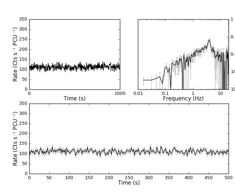
Figure 4.4: Plots of the Class I observation 96420-01-01-00, orbit 0. Top-left: 1000 s lightcurve binned on 2 seconds to show lightcurve evolution. Top-right: Fourier Power Density Spectrum. Bottom: 500 s lightcurve binned on 2 seconds.

In the 2 s binned lightcurve of a Class I observation, there is no structured second-to-minute scale variability. The Fourier PDS of all observations in this class show broad band noise between $\sim 1$–$10$ Hz, as well as a weak QPO (with a $q$-value of $\sim 5$) which peaks at around 5 Hz.

Class II – Figure 4.5

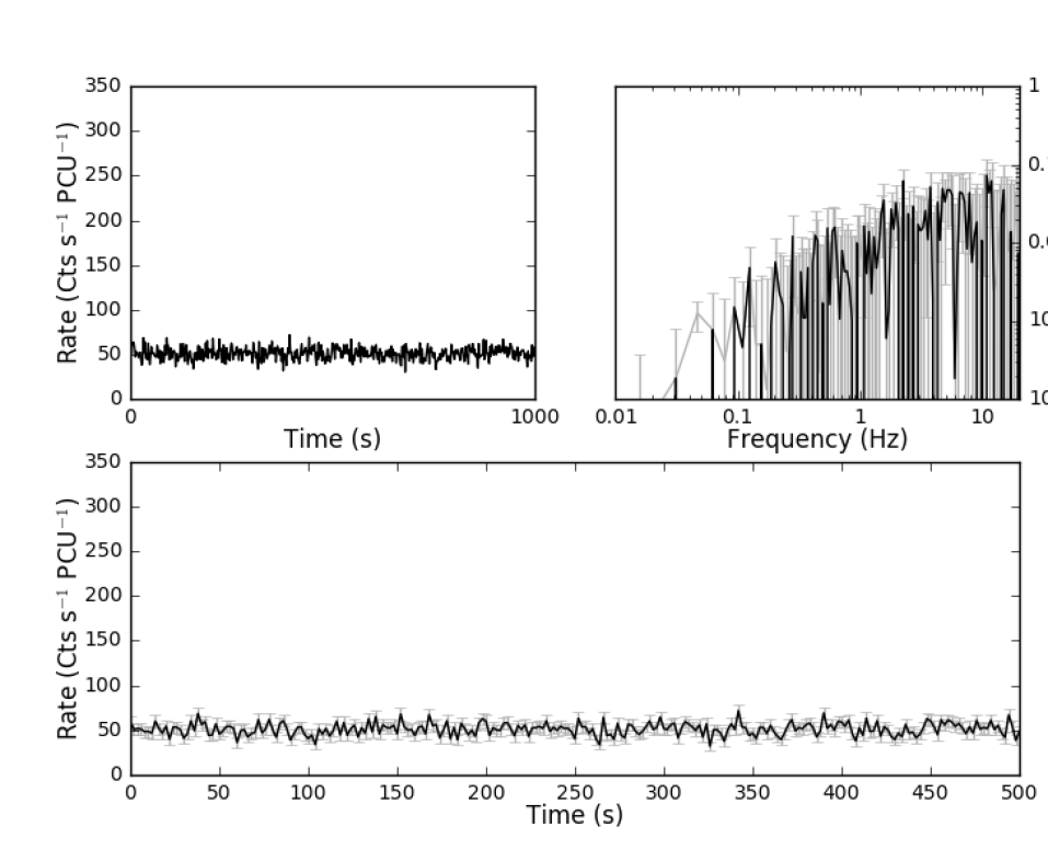
Figure 4.5: Plots of the Class II observation 96420-01-11-00, orbit 0. Top-left: 1000 s lightcurve binned on 2 seconds to show lightcurve evolution. Top-right: Fourier Power Density Spectrum. Bottom: Lightcurve binned on 2 seconds.

Class II observations are a factor of $\sim 2$ fainter in the $L_{T}$ band than Class I observations. They also occupy a different branch in a plot of hardness $H_{A2}$ against intensity (see Figure 4.3, panel c). The PDS shows no significant broad band noise above $\sim 1$ Hz unlike that which is seen in Class I. The $\sim$5 Hz QPO seen in Class I is absent in Class II.

Class III – Figure 4.6

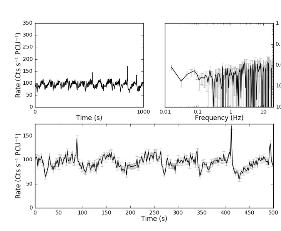
Figure 4.6: Plots of the Class III observation 96420-01-04-01, orbit 0. Top-left: 1000 s lightcurve binned on 2 seconds to show lightcurve evolution. Top-right: Fourier Power Density Spectrum. Bottom: Lightcurve binned on 2 seconds. Note that, to emphasise the behaviour of the lightcurve in this class, I have magnified the 500 s lightcurve y-scale by a factor of 2 compared with the lightcurves presented for other classes.

Unlike Classes I & II, Class III lightcurves show structured flaring, with a peak-to-peak recurrence time of $42$–$80$ s. Most flares consist of a steady $\sim 60$ s rise in count rate and then an additional and sudden rise to a peak count rate at $\gtrsim 200$ cts s^-1 PCU^-1which lasts for $\lesssim$0.5 s before returning to continuum level (I have magnified the y-scaling in the lightcurve of Figure 4.6 to emphasise this behaviour). This sudden rise is not present in every flare; in some observations it is absent from every flare feature. No 5 Hz QPO is present in the PDS and there is no significant variability in the range between $\sim 1\mbox{--}10$ Hz.

As this class has a well-defined periodicity, I folded data in each observation to improve statistics using the best-fit period obtained from generalised Lomb-Scargle Periodogram Analysis; I show a representative Lomb-Scargle periodogram in Figure 4.7. I find an anticlockwise hysteretic loop in the folded HID₁ of all 15 Class III orbits. In Figure 4.8 I show an example of one of these loops.

Figure 4.7: The Lomb-Scargle periodogram of Class III observation 96420-01-19-01, orbit 0, with significance levels of 1, 2 and 3$\sigma$ plotted. The peak at 0.31 Hz was used to define a QPO frequency when folding the data from this observation.

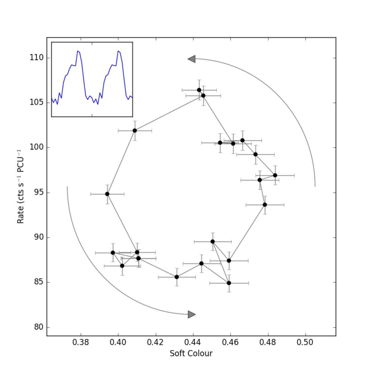
Figure 4.8: The hardness-intensity diagram (HID₁) of the Class III observation 96420-01-04-01, orbit 0. The data have been folded over a period of 79.61 s, corresponding to the peak frequency in the Lomb-Scargle periodogram of this observation. Inset is the folded lightcurve of the same data.

Class IV – Figure 4.9

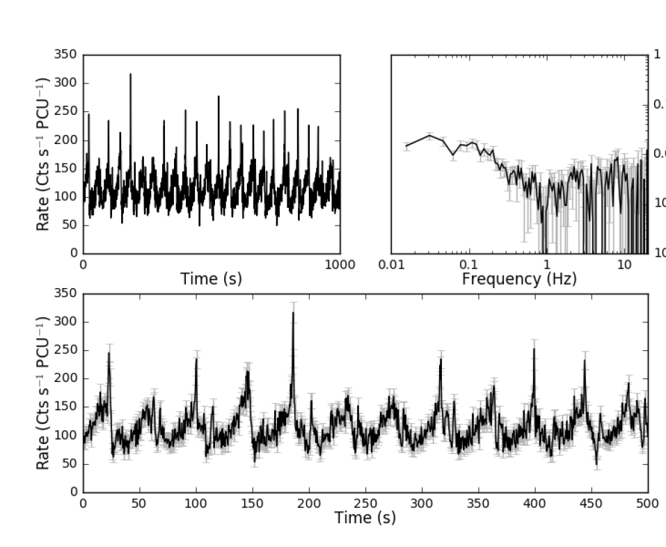
Figure 4.9: Plots of the Class IV observation 96420-01-05-00, orbit 0. Top-left: 1000 s lightcurve binned on 2 seconds to show lightcurve evolution. Top-right: Fourier Power Density Spectrum. Bottom: Lightcurve binned on 0.5 seconds.

The lightcurves in this class show regular variability with a peak-to-peak recurrence time of $25$–$39$ s. I performed peak analysis (see Section 3.2.1) on observations belonging to this class, finding that each flare has a rise time with lower and upper quartile values of $19.5$ and $33.5$ s, a fall time with lower and upper quartile values of $4.6$ and $13.5$ s and a peak count rate of $159$–$241$ cts s^-1 PCU^-1 . There are no significant QPOs in the Fourier PDS above $\sim 1$ Hz.

I folded individual Class IV lightcurves and found anticlockwise hysteretic loops in the HID₁ of 14 out of 30 Class IV observations. In the top panel of Figure 4.10 I show an example of one of these loops. However, I also find clockwise hysteretic loops in 6 Class IV observations, and in 10 orbits the data did not allow us to ascertain the presence of a loop. I provide an example of both of these in the lower panels of Figure 4.10. I note that the structure of clockwise loops are more complex than anticlockwise loops in Class IV, consisting of several lobes rather than a single loop (Figure 4.10, bottom-left).

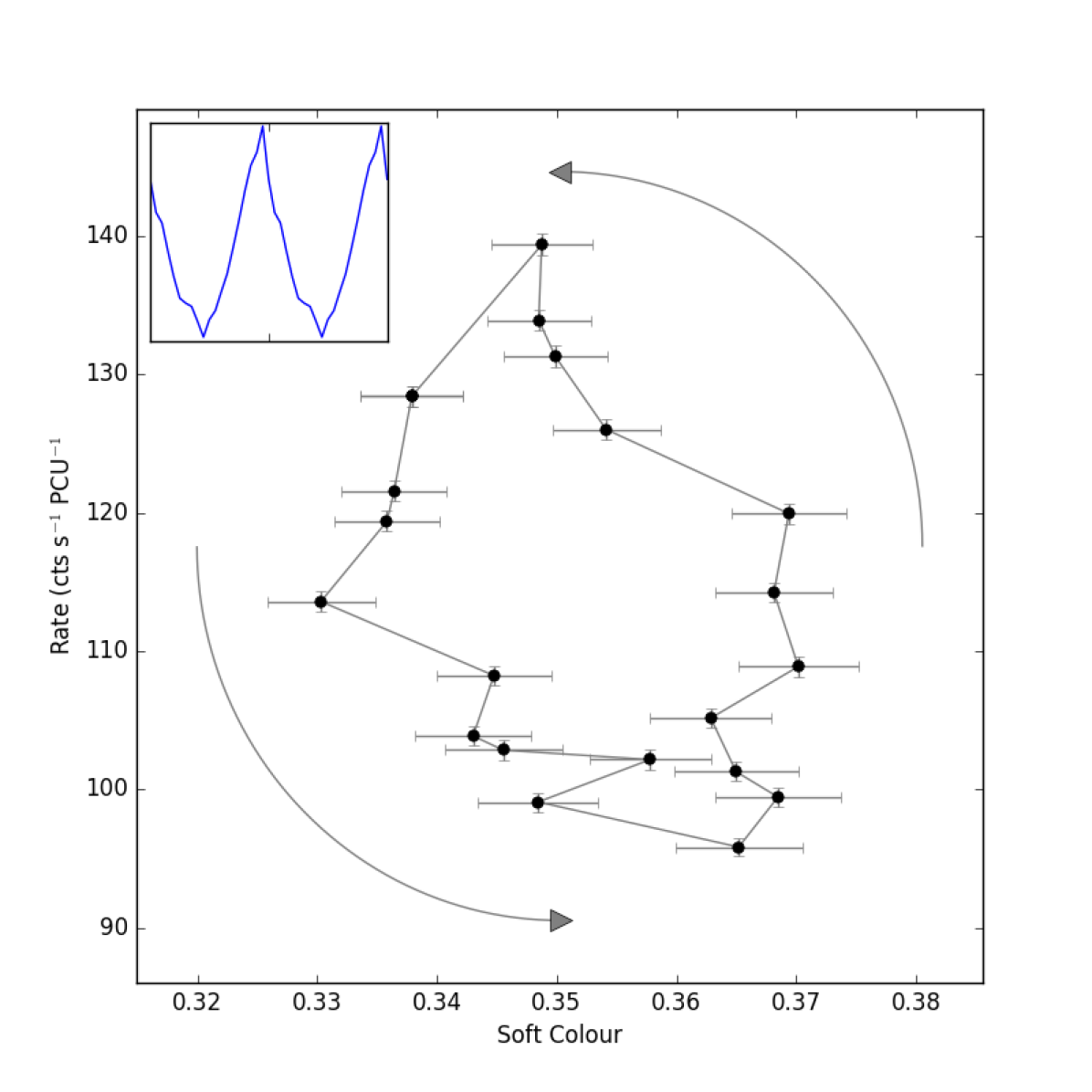
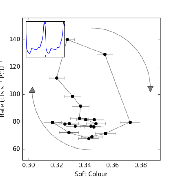
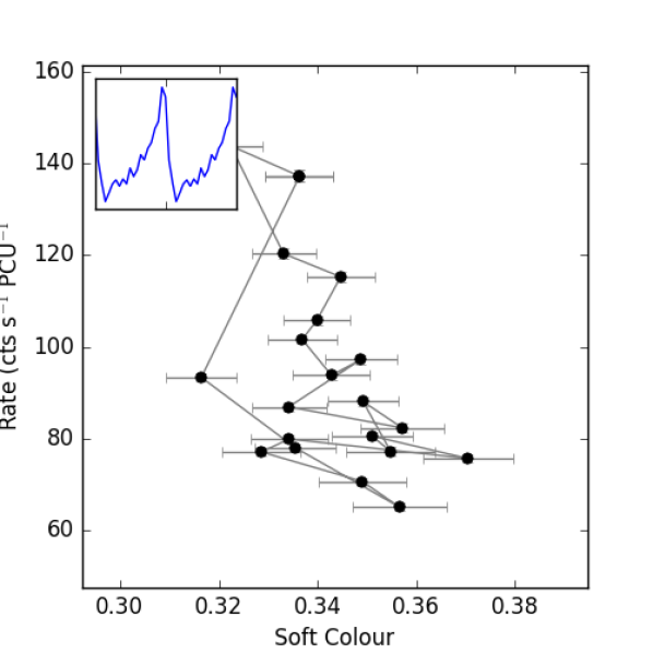
Figure 4.10: Top: The hardness-intensity diagram (HID₁) of the Class IV observation 96420-01-05-00, orbit 0 showing an anticlockwise loop. The data have been folded over a variable period found with the algorithm described in Section 3.2.1. Inset is the folded lightcurve of the same data. Bottom Left: The hardness-intensity diagram of Class IV observations 96420-01-24-02 orbit 0, an example of a clockwise loop. Bottom Right: The hardness-intensity diagram of Class IV observation 96420-01-06-00 orbit 0, in which I was unable to ascertain the presence of a loop.

Compared with Class III, the oscillations in Class IV occur with a significantly lower period, with a mean peak-to-peak recurrence time of $\sim 30$ s compared to $\sim 60$ s in Class III.

In Figure 4.3 I show that Classes III and IV can also be distinguished by average hardness, as Class III tends to have a greater value of $H_{A2}$ than Class IV.

Class V – Figure 4.11

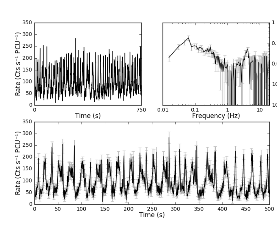
Figure 4.11: Plots of the Class V observation 96420-01-06-03, orbit 0. Top-left: 750 s lightcurve binned on 2 seconds to show lightcurve evolution. Top-right: Fourier Power Density Spectrum. Bottom: Lightcurve binned on 0.5 seconds.

The lightcurves in this class, like in Classes III and IV, show flaring behaviour, with flares separated by a few tens of seconds. At higher frequencies, the PDS shows a prominent QPO centred at $\sim 4$ Hz with as $q$-value of $\sim 3$. There is also significant broad band noise between $\sim 0.1$–$1$ Hz

In Figure 4.12 I show that the flaring in this class is more complex than that seen in Classes III and IV. Class V lightcurves consist of short strongly peaked symmetrical flares (hereafter Type $V_{1}$) and a longer more complex type of flare (hereafter Type $V_{2}$). The Type $V_{2}$ flare consists of a fast rise to a local maximum in count rate, followed by a $\sim 10$ s period in which this count rate gradually reduces by $\sim 50\%$ and then a much faster peak with a maximum count rate between 1 and 2 times that of the initial peak. In both types of flare, I find that the increase in count rate corresponds with an increase in soft colour. The two-population nature of flares in Class V can also clearly be seen in Figure 4.13, where I show a two-dimensional histogram of flare peak count rate against flare duration.

I folded all individual Class V lightcurves, in each case cropping out periods of $V_{2}$ flaring. I find clockwise hysteretic loops in the HID₁ of 30 out of 33 Class V observations, suggesting a lag in the aforementioned relation between count rate and soft colour. In the upper panel Figure 4.14 I present an example of one of these loops. In one observation however, I found an anticlockwise loop in the HID₁ (shown in Figure 4.14 lower-left panel). I was unable to ascertain the presence of loops in the remaining 2 orbits; for the sake of completeness, I show one of these in the lower-right panel of Figure 4.14.

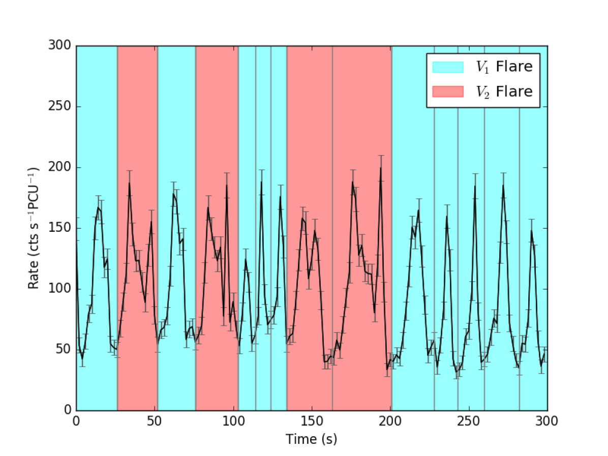
Figure 4.12: A portion of the lightcurve of observation 96420-01-06-03, orbit 0, showing Type $V_{1}$ flares (highlighted in cyan) and Type $V_{2}$ flares (highlighted in red).

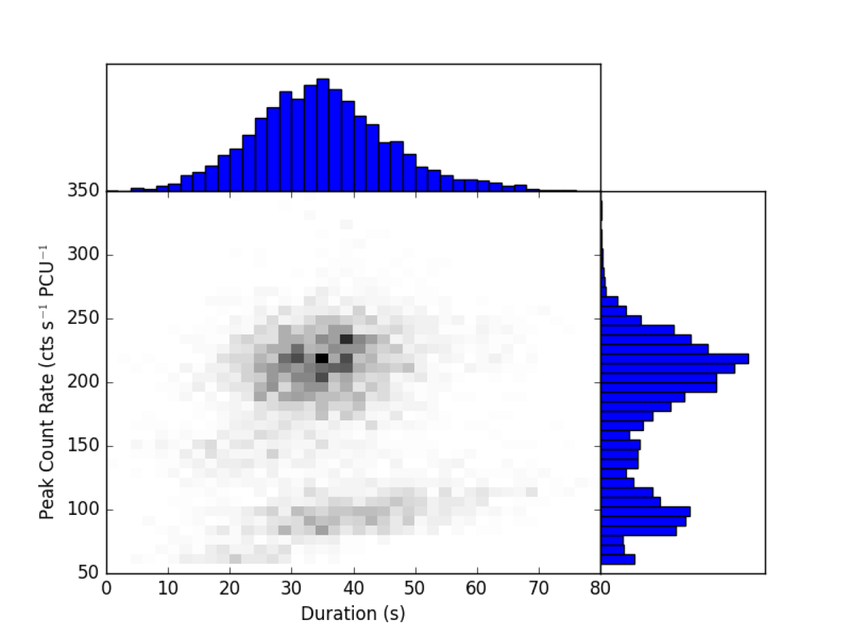
Figure 4.13: Every flare in all observations identified as Class V, plotted in a two-dimensional histogram of flare peak count rate against flare duration to show the two-population nature of these events.

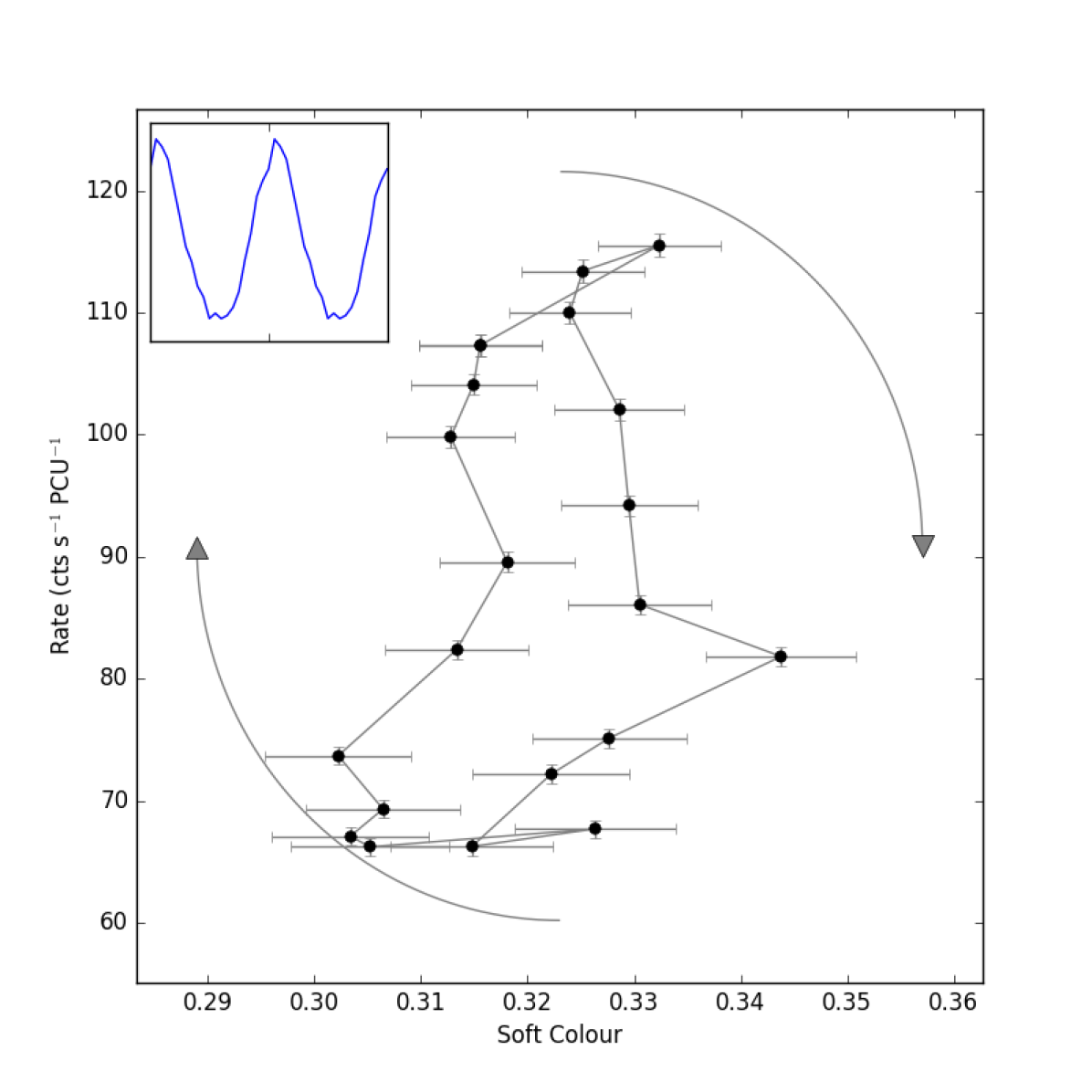
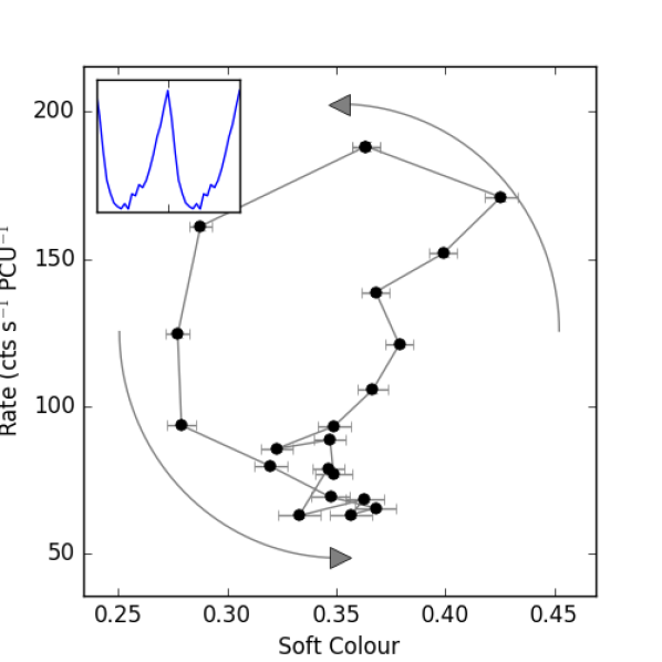
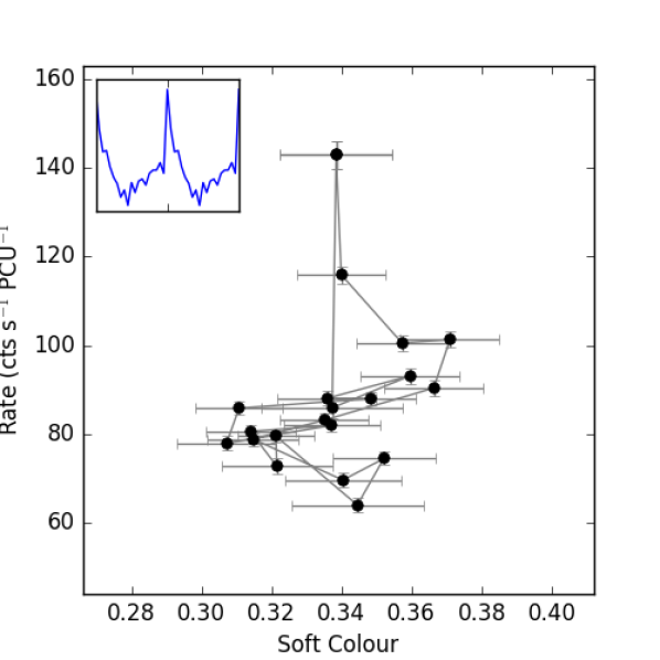
Figure 4.14: Top: The hardness-intensity diagram (HID₁) of a type $V_{1}$ flaring period in Class V observation 96420-01-07-00, orbit 0 showing a clockwise loop. The data have been folded over a variable period found with the algorithm described in Section 3.2.1. Inset is the folded lightcurve of the same data. Bottom Left: The hardness-intensity diagram of Class V observation 96420-01-25-05 orbit 0, an example of an anticlockwise loop. Bottom Right: The hardness-intensity diagram of Class V observation 96420-01-25-06 orbit 0, in which I was unable to ascertain the presence of a loop.

Class VI – Figure 4.15

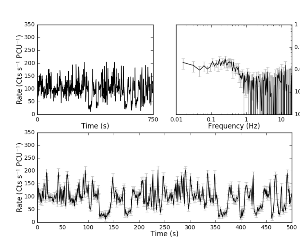
Figure 4.15: Plots of the Class VI observation 96420-01-09-00, orbit 0. Top-left: 750 s lightcurve binned on 2 seconds to show lightcurve evolution. Top-right: Fourier Power Density Spectrum. Bottom: Lightcurve binned on 1 second.

The lightcurves of observations of this class show large dips in count rate; this can be seen in Figure 4.15 at, for example, $t\approx 125$–$150$ s . These dips vary widely in duration, from $\sim 5$ to $\sim 50$ seconds, and the count rate in both $L_{A}$ and $L_{B}$ fall to a level consistent with background. The dips’ rise and fall times are fast, both lasting no longer than a second. They do not appear to occur with any regular periodicity.

Aside from the dips, Class VI observations show other structures in their lightcurves. Large fluctuations in count rate, by factors of $\lesssim 3$, occur on timescales of $\sim 1\mbox{--}5$ s; no periodicity in these oscillations could be found. This behaviour is reflected in the PDS, which shows high-amplitude broad band noise below $\sim 0.5$ Hz with RMS-normalized power (Belloni and Hasinger,, 1990) of up to $\sim 1.1$ Hz^-1. As can be seen in Figure 4.15, this feature takes the form of a broad shoulder of noise which shows either a weak peak or no clear peak at all. The $\sim 5$ Hz QPO seen in the PDS of other classes is not present in Class VI observations.

I attempted to fold all individual Class VI lightcurves, ignoring the sections of data corresponding to the large count rate dips described above. In general, folding lightcurves belonging to this class is difficult; many orbits showed low-amplitude oscillations which were difficult to fold using my flare-finding algorithm (see Section 3.2.1), while many others only showed oscillatory behaviour for a small number of periods between each pair of dips. As such, I only succesfully folded 23 of the 40 Class VI orbits. Of these, 19 showed clockwise loops in the HID₁ (top panel, Figure 4.16), 3 showed anticlockwise loops (bottom-left panel, Figure 4.16). In the remaining 1 observation, the data did not allow us to ascertain the presence of loops (bottom-right panel, Figure 4.16).

Like in Class VI, I note that the clockwise loops in Class VI appear more complex than clockwise loops. Again, the clockwise loop shown in Figure 4.16 appears to have a 2-lobe structure; this is repeated in all clockwise loops found in this class.

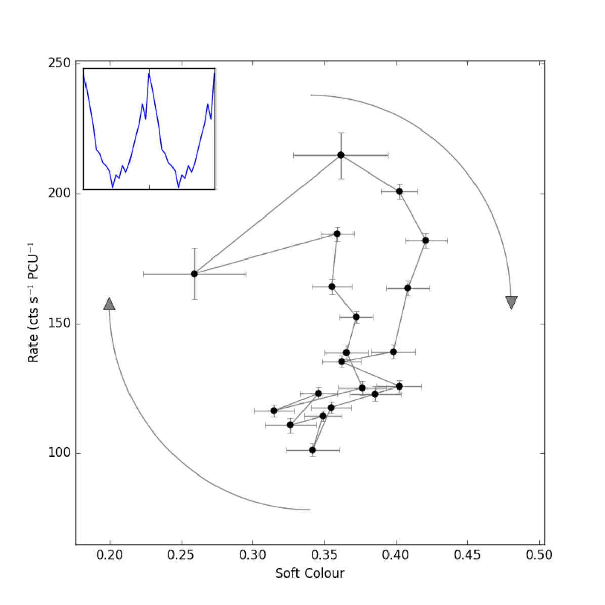
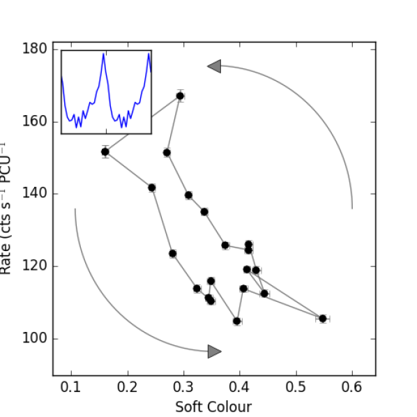
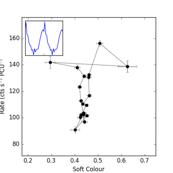
Figure 4.16: Top: The hardness-intensity diagram (HID₁) of the Class VI observation 96420-01-30-03, orbit 0 showing a clockwise loop. The data have been folded over a variable period found with the algorithm described in Section 3.2.1. Inset is the folded lightcurve of the same data. Bottom Left: The hardness-intensity diagram of Class VI observation 96420-01-30-04 orbit 0, an example of an anticlockwise loop. Bottom Right: The hardness-intensity diagram of Class VI observation 96420-01-09-03 orbit 0, in which I was unable to ascertain the presence of a loop.

Class VII – Figure 4.17

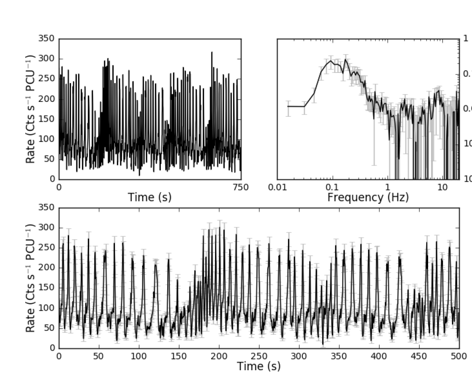
Figure 4.17: Plots of the Class VII observation 96420-01-18-05, orbit 0. Top-left: 750 s lightcurve binned on 2 seconds to show lightcurve evolution. Top-right: Fourier Power Density Spectrum. Bottom: Lightcurve binned on 0.5 seconds.

Class VII shows high-amplitude flaring behaviour with a peak-to-peak recurrence time of $6$–$12$ s. In Figure 4.18 I show a dynamical Lomb-Scargle spectrogram of a Class VII observation, showing that the fast flaring behaviour has a frequency which moves substantially over time. This in turn accounts for the large spread in the value of the flare peak-to-peak recurrence time.

In Figure 4.18 I show that the peak frequency of the QPO also varies in a structured way. I also suggest that the variabilitity of the frequency is itself a QPO with a period of $\sim 150$ s.

At higher frequencies, the PDS shows a weak QPO centred at $\sim 8$ Hz, with a $q$-value of $\sim 2$.

I used my flare-finding algorithm (see Section 3.2.1) to perform variable-frequency folding of Class VII orbits. I find clockwise loops in 9 out of 11 Class VII orbits. In the remaining two observations, the oscillations were extremely fast. As a result, the errors in the HID₁ of these two observations were too large to succesfully select peaks, and I am unable to confirm or reject the presence of loops.

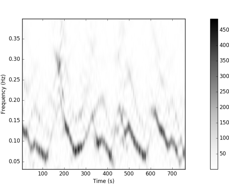
Figure 4.18: A sliding window Lomb-Scargle periodogram of Class VII observation 96420-01-18-05, showing power density spectra from an overlapping 32 s window moved 1 s at a time. The peak frequency of this low frequency QPO itself appears to oscillate with a frequency of $\sim 5$mHz.

Class VIII – Figure 4.19

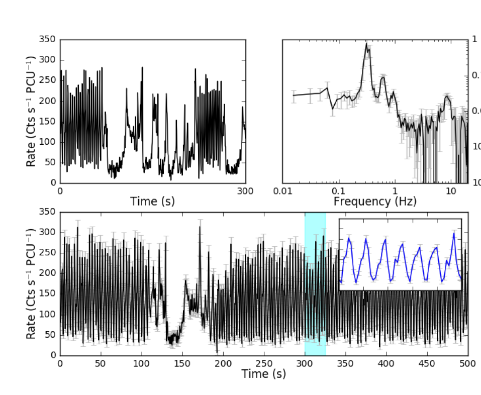
Figure 4.19: Plots of the Class VIII observation 96420-01-19-03, orbit 0. Top-left: 300 s lightcurve binned on 2 seconds to show lightcurve evolution. Top-right: Fourier Power Density Spectrum. Bottom: Lightcurve binned on 0.5 seconds. Inset is a zoom of the 25 s portion of the lightcurve highlighted in cyan, to show the second-scale structure in the lightcurve.

The lightcurve of this variability class shows the dipping behaviour seen in Class VI, as can be seen in Figure 4.19 at $t\approx 125$–$150$ s. The dips are less frequent than in Class VI. The behaviour outside of the dips is dominated by highly structured high-amplitude oscillations consisting of flares with a peak to peak separation of $3.4\pm 1.0$ s. The PDS shows this behaviour as a very significant ($q$-value > 20) QPO; two harmonics of this QPO are also visible. The PDS also shows a strong ($q$-value$\sim 5$) QPO at $\sim 9$ Hz.

I attempted to fold Class VIII lightcurves, ignoring the portions of data corresponding to dips, using my flare-finding algorithm. The high frequency of the dominant oscillation in Class VIII resulted in large errors in the peak times of individual flares, which translated to large errors in all HID₁s; however, I was able to ascertain the presence in loops in 8 out of 16 orbits. All 8 of these loops are clockwise.

Class IX – Figure 4.20

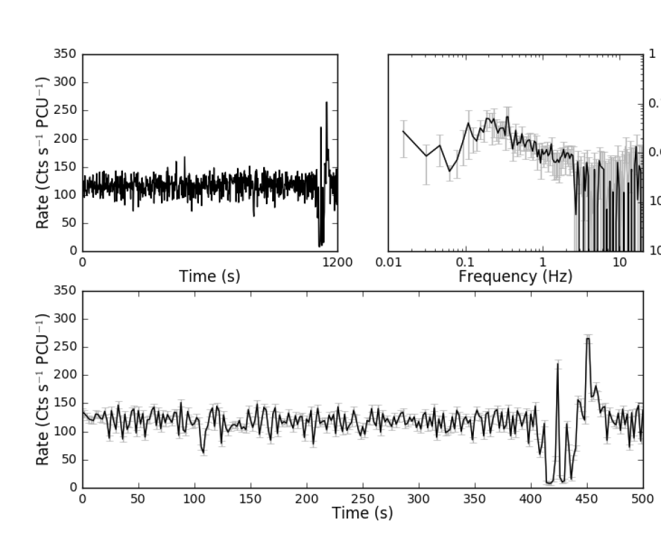
Figure 4.20: Plots of the Class IX observation 96420-01-35-02, orbit 1. Top-left: 1200 s lightcurve binned on 2 seconds to show lightcurve evolution. Top-right: Fourier Power Density Spectrum. Bottom: Lightcurve binned on 2 seconds.

The 1 s lightcurve of a Class IX observation is superficially similar to the lightcurve of a Class I observation, with little obvious structured variability at timescales larger than 2 s; however, large count rate dips like those seen in Classes VI and VIII (e.g. the feature at $t\approx 410$ s in the lightcurve of Figure 4.20) are very occasionally observed. These dips may in turn be coupled to short second-scale flares in which count rate briefly increases by a factor of 2–3.

Outside of these dips and flares, the lightcurve of a Class IX observation is indistinguishable from the lightcurve of a Class I or Class II observation. However, in Figure 4.3, I show that Class IX occupies a very different part of the global $H_{A2}$/$H_{A1}$ colour-colour diagram. Class IX observations show a significantly larger $H_{A2}$ than Class I and II observations, but a significantly lower $H_{A1}$.

The PDS reveals significant broad band noise peaked at $\sim$0.3 Hz, and the $\sim 5$ Hz QPO seen in other classes is absent. Altamirano and Belloni, (2012) discovered high frequency ($\sim 66$ Hz) QPOs in observations corresponding to this variability class.

4.2.3 Swift

Observations with Swift took place throughout the 2011-2013 outburst of IGR J17091-3624. Between MJDs 55622 and 55880, 17 Swift/XRT were at least partly simultaneous with an RXTE observation, corresponding to at least one observation of all 9 classes. In each case, the Swift and RXTE lightcurves were similar. The remainder of the Swift/XRT observations during this time were also consistent with belonging to one of my nine classes. Given that the RXTE data have higher count rate and time resolution, I do not further discuss the Swift observations taken before MJD 55880.

Between MJD 55952 and 56445, Swift observations showed IGR J17091-3624 decreasing in flux. For all observations longer than 500 s, I rebinned the lightcurves to 10 s and calculated the fractional RMS. I find the lower and upper quartiles of the fractional RMS in these measurements to be 18.3% and 21.7% respectively. INTEGRAL observations taken as part of a scan programme of the Galactic Plane (Fiocchi et al.,, 2012) and reported by Drave et al., (2012) suggest that IGR J17091-3624 returned to the hard state between MJDs 55952 and 55989. Therefore these observations sample IGR J17091-3624 in the hard state.

4.2.4 INTEGRAL

The results of the INTEGRAL/IBIS analysis are presented in Table 4.4. C.B. finds clear detections of IGR J17091-3624 in all energy bands during the hardest period (MJD 55575–55625) of the 2011–2013 outburst. Conversion from detected counts to flux was achieved using an INTEGRAL/IBIS observation of the Crab taken between MJD 57305.334 and 57305.894. Conversion from Crab units to standard flux units was obtained by conversion factors listed in Bird et al., (2016) and Bazzano et al., (2006).

Energy	Intensity	Significance	Exposure	Flux	Flux
(keV)	(cts/s)	$\sigma$	(ks)	(mCrab)	(10-10ergs s-1 cm-2)
20–40	12.39$\pm$0.05	247	115	93.5$\pm$0.38	7.08$\pm$0.03
40–100	7.06$\pm$0.05	157	163	83.5$\pm$0.60	7.87$\pm$0.06
100–150	1.05$\pm$0.03	40	173	66.9$\pm$1.91	2.14$\pm$0.06
150–300	0.23$\pm$0.03	7.6	179	46.6$\pm$5.96	2.24$\pm$0.29

Table 4.4: Results from the IBIS/ISGRI analysis of the 2011–2013 Outburst of IGR J17091. The 20–40 keV flux is given in units of mCrab and (10^-11 ergs s^-1 cm^-2). Conversion between counts and mCrab was obtained using an observation of the Crab taken during Revolution 1597 between MJD 57305.334 and 57305.894 and the conversion factors of Bird et al., (2016) and Bazzano et al., (2006).

Comparing these results with those of Bazzano et al., (2006), we see that IGR J17091 is detected for the first time above 150 keV with a detection significance of 7.6 $\sigma$, corresponding to a flux of $2.24\pm 0.29\times 10^{-10}$ ergs s^-1 cm^-2 (Figure 4.21).

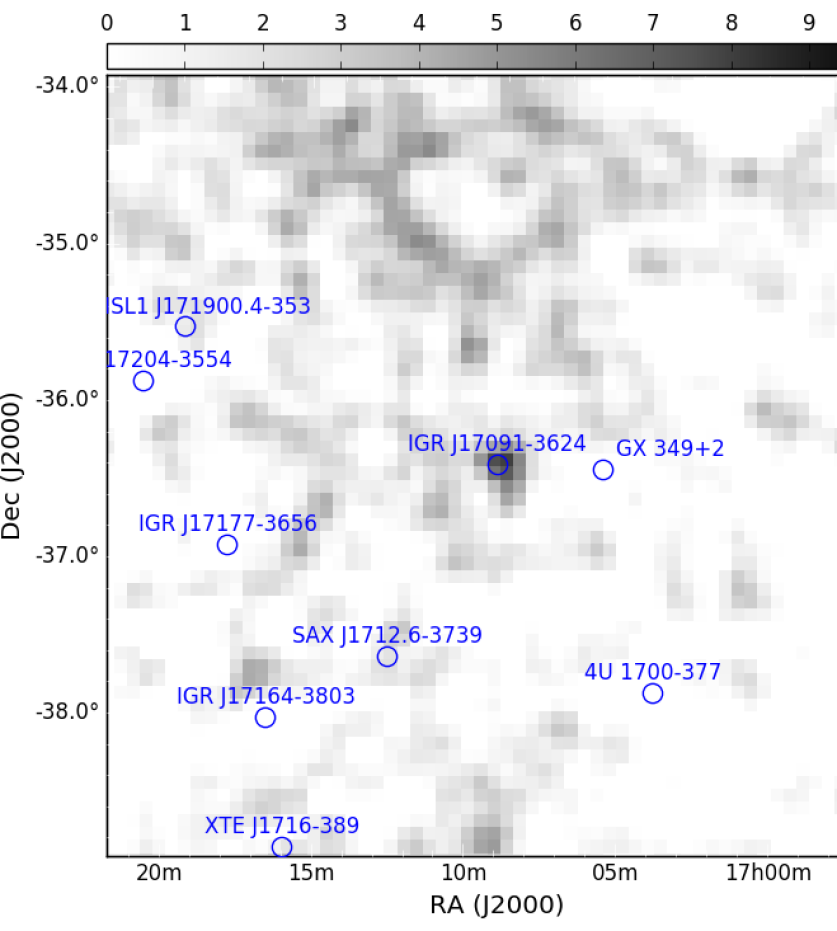
Figure 4.21: INTEGRAL/ISGRI 150–300 keV significance map of a $2^{\circ}$ region centred on the position of IGR J17091-3624, showing the first significant detection of this source above 150 keV. The detection significance is 7.6 $\sigma$.

4.2.5 Chandra

In Figure 4.22, I present lightcurves from the three Chandra observations considered in this chapter (see also Table 4.1 for details of these observations).

Figure 4.22: 1 ks segments of lightcurves taken from Chandra observations 12505, 12405 and 12406, showing Class I, Class VII and Class IX variability respectively. The lightcurve presented for observation 12505 is for the energy range 0.06-10 keV, while the other two lightcurves are for the energy range 0.5-10 keV. All three lightcurves are binned to 0.5 s.

Observation 12505 was performed within 24 hours of RXTE observation 96420-01-02-01, which showed Class I variability. No structured variability is seen in the lightcurve of ObsID 12505 (Figure 4.22, upper panel), which is consistent with Class I. Note that I consider the energy range 0.06-10 keV for this observation but 0.5-10 keV for observations 12405 and 12406.

Observation 12405 was performed within 24 hours of RXTE observation 96420-01-23-03, which showed Class V variability. The two observations were not simultaneous; ObsID 12405 began $\sim 8.4$ ks after ObsID 96420-01-2303 finished. The lightcurve of Chandra ObsID 12405 (shown in Figure 4.22, middle panel) shows a mean count rate of 41 cts s^-1. The lightcurve shows fast flaring behaviour (with a recurrence time on the order of 10s of seconds) in which the frequency changes widely on timescales of $\sim 1000$ s. This observation strongly resembles a Class VII lightcurve, but with its characteristic timescales increased by a factor of $\sim 4$. This leads to the possibility that the low number of Class VII RXTE observations I identify is due to a selection effect; we would not have been able to see this observation’s long-term Class VII-like behaviour if the observation had been shorter than $\sim 2$ ks.

Observation 12406 was performed within 24 hours of RXTE observation 96420-01-32-06, which showed Class IX variability. The lightcurve presented for Chandra ObsID 12406 shows a mean count rate (36 cts s^-1), which is consistent with IGR J17091 being harder in this observation than in Observation 12505. This, combined with the lack of variability seen in its lightcurve, suggests that Observation 12505 is consistent with Class IX.

4.2.6 XMM-Newton

In Figure 4.23 I show lightcurves from two XMM-Newton observations. The lightcurve of XMM-Newton observation 0677980201, shown in the upper panel of Figure 4.23, shows the regular flares characteristic of Class IV variability. A simultaneous RXTE observation (ObsID 96420-01-05-000) also showed Class IV variability.

Figure 4.23: Lightcurves of XMM-Newton observations 0677980201 and 0700381301, showing Class IV variability and the hard state respectively. Both lightcurves binned to 2 s. Data for observation 0677980201 is taken from EPIC-MOS2 and data for observation 0700381301 is taken from EPIC-pn.

XMM-Newton observation 070038130, shown in the lower panel of Figure 4.23, was made after the end of RXTE observations IGR J17091-3624. As such it cannot be compared with contemporaneous RXTE data. The 5 s binned lightcurve shows no apparent variability, but a Fourier PDS of the observation (shown in Figure 4.24) reveals a QPO centred at around $\sim 0.15$ Hz and a broad band noise component at lower frequencies. Drave et al., (2012) reported that IGR J17091 transited to the hard state in February 2012, seven months before this observation was taken. As such, I find that observation 0677980201 samples the hard state in IGR J17091 and is thus beyond the scope of my set of variability classes.

Figure 4.24: RMS-normalised co-added power density spectra of XMM-Newton observation 0700381301 and Suzaku observation 407037010. Both observations were taken simultaneously on September 29 2012 (MJD 56199). I sample observation 0700381301 up to a frequency of 10 Hz, while the 2 s time resolution of observation 407037010 results in a Nyquist frequency of 0.25 Hz.

4.2.7 Suzaku

The two Suzaku observations of IGR J17091-3624 considered here, ObsIDs 407037010 and 407037020, were performed during the 2nd and 3rd re-flares of the hard state phase of the 2011–2013 outburst. ObsID 407037010 was taken simultaneously with XMM-Newton observation 0700381301. The XIS 0 count rates are 7.8 cts s^-1 and 2.5 cts s^-1 respectively.

Neither lightcurve shows ‘heartbeats’ or any other type of GRS 1915-like variability. However, K.Y. and I find evidence of a low frequency QPO feature at $\sim$0.15 Hz in the ObsID 407037010; this QPO is also seen in XMM-Newton observation 0700381301 (Figure 4.24). The presence of a QPO below 1 Hz and flat-topped power density spectrum confirm that IGR J17091 was in the hard state at this time.

4.3 Discussion

Using observations from XMM-Newton, RXTE and Chandra, I describe the complex variability seen in IGR J17091 as a set of nine variability ‘classes’, labelled I to IX. These classes are distinguished from each other by values of upper and lower quartile (i.e. 25^th and 75^th percentile) count rates, mean RMS, the presence of QPOs in Fourier PDS, the shape of flare and dip features in the lightcurve and the presence of loops in the 6–16/2–6 keV hardness-intensity diagram HID₁. See Section 4.2 for a full description of these classes.

The classification of some observations is clearer than others. Some orbits were too short to definitively quantify the behaviour of the source, whereas some other orbits contain a transition between two classes. An example lightcurve showing a transition from Class III to Class IV is presented in Figure 4.25.

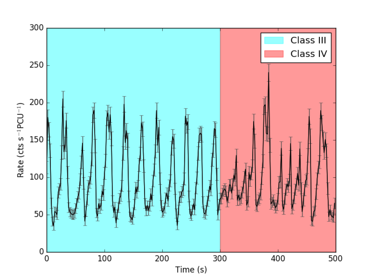
Figure 4.25: A lightcurve of observation 96420-01-06-02, orbit 0, showing a transition in behaviour between Class III (in cyan, see Section 4.2.2) and Class IV (in red, see Section 4.2.2).

My set of classes is analogous to, but not based upon, the set of variability classes defined by Belloni et al., 2000 to describe the behaviour of the similarly complex LMXB GRS 1915. This ensures that my set of classes is not biased by an a priori assumption that the two objects are similar. However if we do assume that wide range of variability seen in these two objects are driven by the same physical processes, a direct comparison between the variability classes in the two systems can further our understanding of the physics that drive these exotic objects.

4.3.1 Variability Classes: IGR J17091 vs. GRS 1915

As observations of IGR J17091 and GRS 1915 suffer from different values of interstellar absorption $N_{H}$, I cannot directly compare the absolute colours of these two objects. However, I can compare the evolution of colour both over time and as a function of count rate. I therefore use these parameters, along with power spectra and lightcurve morphology, when comparing GRS 1915 with IGR J17091.

For seven of my classes, I was able to assign the closest matching class described by Belloni et al., 2000 for GRS 1915 (see Table 4.5). I am unable to find analogues to my classes VII and VIII in observations of GRS 1915, and I suggest that these classes are unique to IGR J17091.

Table 4.5: The nine variability classes of IGR J17091-3624, showing the name of the closest corresponding variability class in GRS 1915+105. The names of GRS 1915+105 classes are taken from Belloni et al., (2000), where more detailed descriptions can be found. Eight additional classes of GRS 1915+105 have been described; I do not find analogies to these classes in IGR J17091-3624.

IGR J17091-3624 Class	GRS 1915+105 Class
I	$\chi$
II	$\phi$
III	$\nu$
IV	$\rho$
V	$\mu$
VI	$\lambda$
VII	None
VIII	None
IX	$\gamma$

Below, I evaluate my mapping between GRS 1915 and IGR J17091 classes, and interpret the differences between each matched pair.

Classes I and II – Figures 4.4, 4.5

Classes I and II both show low count rates and little structure in their lightcurves. The two classes in GRS 1915 that also show this lightcurve behaviour are Class $\chi$ and Class $\phi$. Belloni et al., 2000 differentiate between Classes $\phi$ and $\chi$ based on the hard colour (corresponding to $C_{2}$), as Class $\chi$ has a significantly higher value for this colour than Class $\phi$.

Data from RXTE  indicates that the transition from the hard state to the soft intermediate state between MJDs 55612 and 55615 (Drave et al.,, 2012). This was confirmed by a radio spectrum taken on MJD 55623 which was consistent with an observation of discrete ejecta (Rodriguez et al., 2011a, ). This observation of discrete ejecta at the transition between the hard state and the intermediate state has been reported in other LMXBS (e.g. XTE J1550-564, Rodriguez et al.,, 2003), and has also been associated with transitions to the $\chi$ Class in GRS 1915 (Rodriguez et al.,, 2008, see also review by Fender,, 2006).

Using Fourier PDS, I conclude that Class I is analogous to Class $\chi$ in GRS 1915, while Class II is analogous to Class $\phi$. In Class $\chi$ observations of GRS 1915, broad band noise between $\sim 1-10$ Hz and a QPO at around 5 Hz are seen in the PDS. I find that both of these are present in Class I observations of IGR J17091. On the other hand, I find that Class $\phi$ observations of GRS 1915 do not show this broad band noise, and show either a weak ($q$-value $\lesssim 3$) QPO at $\sim 5$ Hz or no QPO at all. I find that the weak QPO and lack of broad band noise are also seen in the PDS of Class II observations.

Classes III and IV – Figures 4.6, 4.9

Classes III and IV both show highly regular flaring activity in their lightcurves, but they differ in terms of timescale and pulse profile. As can be seen in lightcurves in Figure 4.9, flares in Class IV occur every $\sim 32$ s and are nearly identical to each other in shape. On the other hand, as can be seen in Figure 4.6, flares in Class III occur every $\sim 61$ s and may or may not end in a much faster sharp peak which is never seen in Class IV. In Figure 4.26 I show a two-dimensional histogram of flare peak count rate against flare duration, showing all flares in all observations classified as Class III or Class IV. In this figure, I can see that flares tend to group in one of two regions in count rate-duration space; a region between $\sim 90\mbox{--}110$  cts s^-1 PCU^-1and $\sim 35\mbox{--}55$ s, corresponding to flares seen in Class III, and a region between $\sim 150\mbox{--}250$  cts s^-1 PCU^-1and $\sim 20\mbox{--}55$ s, corresponding to flares seen in Class IV. From this plot, I conclude that the flares seen in Class III exist in a different population to the flares seen in Class IV.

The GRS 1915 classes that show behaviour most similar to these are $\rho$ and $\nu$; both produce similar structures in their lightcurve, but Class $\nu$ is differentiated from Class $\rho$ by the presence of a secondary count rate peak which occurs $\sim 5$ s after the primary (Belloni et al.,, 2000).

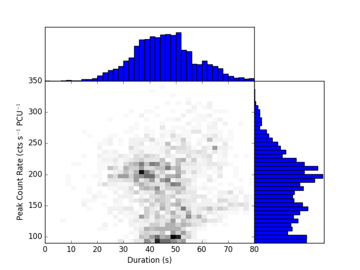
Figure 4.26: Every flare in all observations identified as Class III or Class IV, plotted in a two-dimensional histogram of flare peak count rate against flare duration to show the two-population nature of these events. Flares belonging to Class IV occupy the distribution at higher peak rate and lower duration, whereas flares belonging to Class III occupy the distribution at lower peak rate and higher duration.

The secondary peak is present in most Class III observations and some Class IV observations (Figure 4.27), suggesting that both classes consist of a mix of $\rho$-like and $\nu$-like observations. However, the poor statistics sometimes make the presence of this secondary peak difficult to detect. As such, I do not use the presence or absence of this peak as a criterion when assigning classes. Instead I choose to separate Classes III and IV based on the larger-scale structure in their lightcurves (see Section 4.2.2). Due to the aforementioned difference in burst populations between the two classes, I suggest that classes III and IV do represent two distinct classes rather than a single class with a period that drifts over time. I suggest that Classes $\rho$ and $\nu$ in GRS 1915 could also be re-partitioned in this way.

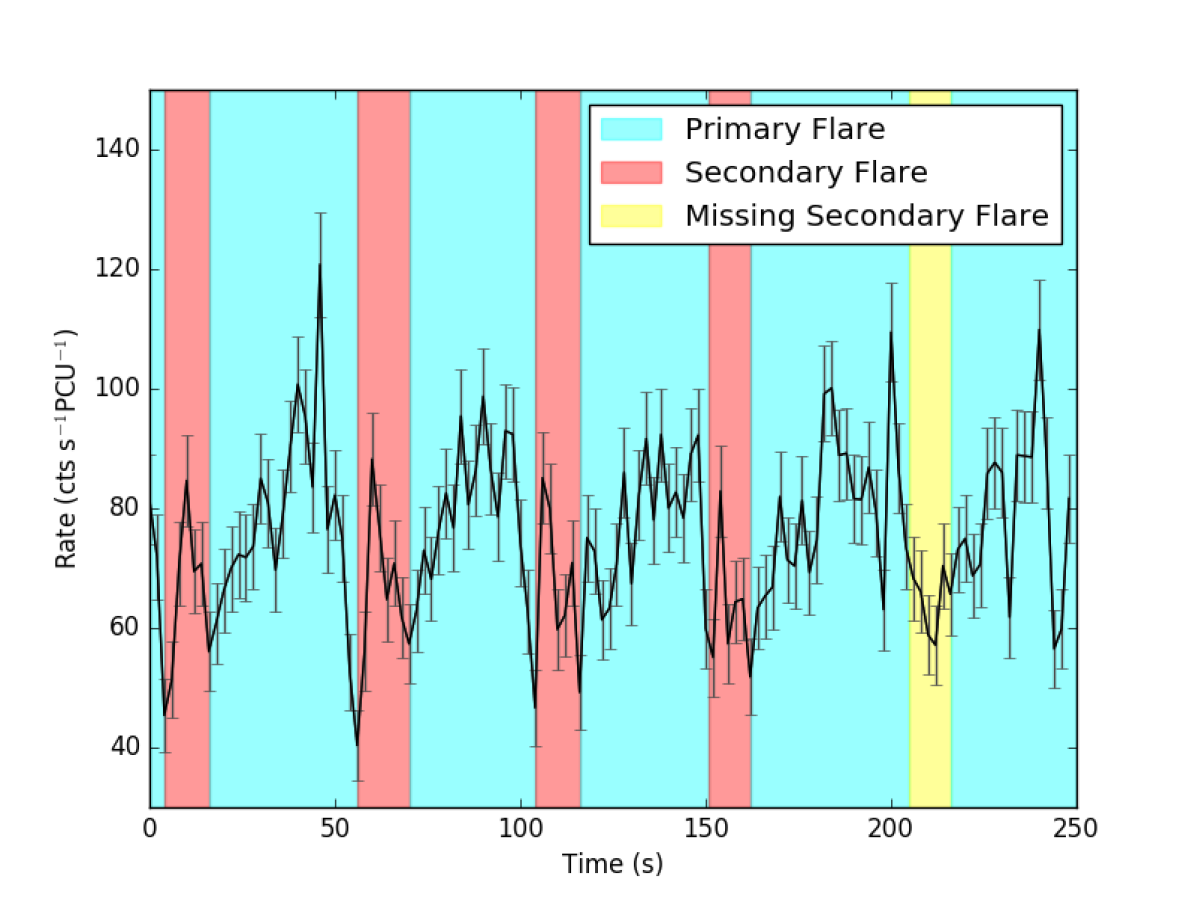
Figure 4.27: Lightcurve from Class III observation 96420-01-10-01 of IGR J17091-3624, with pairs of primary and secondary count rate spikes highlighted in cyan and red respectively. The yellow region highlights a primary count rate spike that did not produce a secondary.

However, HID₁ loops are found to generally execute in an anticlockwise direction in Classes III and IV (previously noted by e.g. Altamirano et al., 2011b, ); the opposite direction to the clockwise loops in Classes $\rho$ and $\nu$ reported by e.g. Belloni et al.,, 2000 and repeated by us using the same method I apply to data from IGR J17091-3624 (see Section 4.1). This suggests that Classes III and IV could be generated by a different physical mechanism to Classes $\rho$ and $\nu$. Alternatively, Classes III and IV could be generated by the same mechanism as $\rho$ and $\nu$ if some other unknown process was able to alter the spectral evolution of flares in these classes.

Class V – Figure 4.11

The lightcurve of a Class V observation appears similar to that of a Class $\mu$ observation of GRS 1915, as both are characterised by rapid $\rho$-like flares which occur less regularly than in Class $\rho$. In addition to this, flares in Class $\mu$ fall into two clear populations, as do the flares in Class V. However, significant differences exist between Class V and Class $\mu$. Class $\mu$ observations are characterised by long ($\sim 100$ s) excursions to plateaus of high count rate, a behaviour which is not seen in any Class V observation thus far.

I note that the HID₁ in Class V observations displays a loop in the clockwise direction; the opposite direction to the looping seen in Classes III and IV but the same direction seen in Class $\mu$.

Regarding the two-population nature of flares seen in this class (see Section 4.2.2), I suggest that V₂ flares may simply be two V₁ flares that occur close together in time, such that the second flare starts during the decay of the first flare. This would result in an apparent two-peaked flare structure, as we see in type V₂ flares. This interpretation also accounts for the bimodal distribution of flare duarations shown in the 2D histogram of Figure 4.13, as this could be caused by the misinterpretation of two-flare V₂ events as a single event. This also accounts for the Gaussian distribution of peak flare intensities seen in Figure 4.13), as the constituents of each V₂ event would be from the same population as V₁ flares.

Class VI – Figure 4.15

Class VI is dominated by long flaring periods which separate periods of low count rate, as can be seen in the lightcurve presented in Figure 4.15. Similar behaviour is seen in the lightcurves of observations of GRS 1915 belonging to Classes $\lambda$ and $\omega$ (Klein-Wolt et al.,, 2002). However, the long count rate ‘dips’ are far less regular in Class VI than in Classes $\lambda$ and $\omega$, and I also note long periods of medium count rate during which neither flares nor dips occur. This variability class is noted by Pahari et al., (2012) who suggest that this class is unique to IGR J17091. However, Pahari et al., 2013b show that, in a plot of burst decay time against burst rise time, Classes VI and $\lambda$ fall in a straight line, suggesting a similar physical origin for both.

While it is cetainly true that Class VI is not a perfect analogue of either Class $\lambda$ or Class $\omega$  Class VI only differs noticeably from Class $\lambda$ during the extended low-variability portions of its lightcurves. As such, I associate Class VI with Class $\lambda$.

Class VII – Figure 4.17

I am unable to find an analogue of Class VII in observations of GRS 1915. This class, and its apparent uniqueness, have previously been noted by Pahari et al.,, 2012. Pahari et al., found that the $C_{2}$ hard colour in this class increases during count rate dips and decreases during count rate peaks. Here I reproduced the results of Pahari et al., and found that the anti-correlation between hard-colour and intensity is not physical, but due to the definition of $C_{2}$: the count rate in band $L_{C}$ is approximately constant and consistent with background, and therefore $C_{2}=L_{C}/L_{A}\propto L_{A}^{-1}$, which will naturally anticorrelate with intensity.

Class VIII – Figure 4.19

I am unable to find an analogue of Class VIII in observations of GRS 1915. When it is flaring, the lightcurve waveform is similar to that seen in Class $\rho$, with rapid regular spikes in count rate. The lightcurve also shows irregular dips in count rate similar to those seen in Class VI and in Class $\lambda$ in GRS 1915.

However, the amplitude of the flares in Class VIII is much larger, and the frequency much higher, than in Classes VI or $\lambda$. The amplitude of the flares in Class VIII can approach $\sim 350$ cts s^-1 PCU^-1, while the flare separation time of 4–5 s makes Class VIII the fastest flaring activity seen in any class of IGR J17091 or GRS 1915. As such, I consider this variability class distinct from both Class VI and Class $\lambda$.

Class IX - Figure 4.20

Class IX is defined by long periods of high amplitude but unstructured variability (with a broad peaked noise component in the Fourier spectrum peaked at $\sim$0.3 Hz) punctuated with infrequent irregular short-duration ‘spikes’ in which the count rate increases by a factor of $\sim 2$–$3$. A similarity between this Class and Class $\gamma$ in GRS 1915 has been previously noted by Altamirano and Belloni, (2012). However, the irregular spikes seen in some Class IX lightcurves are not reproduced in Class $\gamma$ lightcurves of GRS 1915.

4.3.2 General Comparison with GRS 1915+105

Overall, variability in IGR J17091 tends to be faster than structurally similar variability in GRS 1915, as can be noted in Classes III and IV compared to Classes $\rho$ and $\nu$ (see also Altamirano et al., 2011b, ). Additionally, IGR J17091 also displays highly structured variability unlike anything yet seen in GRS 1915, with classes VII and VIII in particular showing very fine detail in their lightcurves.

In total I find 2 variability classes which are seen in IGR J17091 but not in GRS 1915, compared with 8 that are seen in GRS 1915 but not in IGR J17091. As relatively little data exists on GRS 1915-like variability in IGR J17091, the presence of classes in GRS 1915 that are not seen in IGR J17091 could simply be an observational effect. It is unknown how long each variability class lasts for and, as such, additional variability classes could have occurred entirely while IGR J17091 was not being observed. However, GRS 1915 has displayed variability classes consistently since its discovery in 1992 (see e.g. see Huppenkothen et al.,, 2017), implying that the two classes seen only in IGR J17091 are either completely absent in GRS 1915 or that they occur with a much lower probability. In either case, this implies physical differences between methods of generating GRS 1915-like variability in the two objects.

As noted in section 4.3.1, variability classes seen in both IGR J17091 and GRS 1915 show differences between the different objects. In particular, I note the presence of irregular flares in Class IX which are not seen in the analogous Class $\gamma$. If these classes are indeed generated by the same processes in both objects, the differences between them must represent physical differences between the objects themselves.

It has previously been noted that, while the hardness ratios in IGR J17091 and GRS 1915 during $\rho$-like classes are different, the fractional hardening between the dip and peak of each flare is consistent with being the same in both objects (Capitanio et al.,, 2012). This suggests that the same physical process is behind the ‘heartbeats’ seen in both objects.

I note the presence of hysteretic HID₁ loops in some classes of both objects. Although these loops are always clockwise in GRS 1915, they can be executed in either direction in IGR J17091. Classes in IGR J17091 that show loops all have a preferred loop direction: anticlockwise in Classes III and IV and clockwise in classes V, VI, VII and VIII. In cases where the loop direction was opposite to that expected for a given class, loop detections were generally only marginally significant. In particular, I note that Classes IV and V tend to show loops in opposite directions, despite the similarities between their lightcurves and the $\rho$, $\nu$ and $\mu$ classes in GRS 1915. The fact that IGR J17091 can show HID₁ loops in both directions suggests that an increase in soft emission can either precede or lag a correlated increase in hard emission from IGR J17091. Whether soft emission precedes or lags hard emission is in turn is dependent on the variability class.

There are also non-trivial similarities between variability in the two objects. I note the presence of a $\sim 5$ Hz QPO in many of the classes seen in IGR J17091, and this same 5 Hz QPO is seen in data from GRS 1915. Similarly Altamirano and Belloni, (2012) reported the discovery of a 66 Hz QPO in IGR J17091; a very similar frequency to the 67 Hz QPO observed in GRS 1915 (Morgan et al.,, 1997). It is not clear why these QPOs would exist at roughly the same frequencies in both objects when other variability in IGR J17091 tends to be faster.

4.3.3 Comparison with the Rapid Burster

In 2015, Bagnoli and in’t Zand, (2015) reported the discovery of two GRS 1915-like variability classes in the neutron star binary MXB 1730-335, also known as the ‘Rapid Burster’. Specifically, Bagnoli and in’t Zand, (2015) note the presence of variability similar to Classes $\rho$ and $\theta$ in GRS 1915.

Class $\theta$-like variability, seen in RXTE observation 92026-01-20-02 of the Rapid Burster, is not closely matched by any of the classes I identify for IGR J17091. However, the lightcurves of a Class $\theta$ observation feature large dips in count rate similar to those seen in Classes VI and VIII in IGR J17091.

Conversely, Class $\rho$-like variability is seen in all three objects. Bagnoli and in’t Zand, (2015) note that the variability of the $\rho$-like flaring is slower in the Rapid Burster than in either GRS 1915 or IGR J17091. It has previously been suggested that the maximum rate of flaring in LMXBs should be inversely proportional to the mass of the compact object (e.g. Belloni et al., 1997b, ; Frank et al.,, 2002). In this case, the fact that variability is faster in IGR J17091 than in GRS 1915 could simply be due to a lower black hole mass in the former object (Altamirano et al., 2011b, ). However if variability in the Rapid Burster is assumed to be physically analogous to variability in these two black hole objects, then a correlation between central object mass and variability timescale no longer holds.

4.3.4 Comparison with Altamirano et al., 2011b,

Altamirano et al., 2011b identify 5 GRS 1915 variability classes in a subset of observations from the 2011-2013 outburst of IGR J17091: six of these observations are presented in Table 4.6 along with the best-fit GRS 1915 class that I assign it in this chapter (see also Table 4.5).

Table 4.6: The six IGR J17091-3624 ObsIDs explicitly classified in Altamirano et al., 2011b . I also present the GRS 1915 class with which I implicitly label each ObsID in this chapter.

ObsID	Altamirano et al.	My Class
	Class	(implied)
96420-01-04-03	$\alpha$	$\rho/\nu$
96420-01-05-00	$\nu$	$\rho/\nu$
96420-01-06-00	$\rho$	$\rho/\nu$
96420-01-07-01	$\rho$	$\mu$
96420-01-08-03	$\beta/\lambda$	$\lambda$
96420-01-09-06	$\mu$	$\lambda$

I acknowledge differences between the classifications assigned by me and by Altamirano et al., 2011b . I ascribe these differences to the different approaches we have used to construct our classes. In particular while I have constructed an independent set of variability classes for IGR J17091 which I have then compared to the Belloni et al., classes for GRS 1915, Altamirano et al., 2011b applied the Belloni et al., classes for GRS 1915 directly to IGR J17091.

In general, the variability classes I find to be present in IGR J17091 are broadly the same as those noted by Altamirano et al., 2011b . I do not associate any class with Class $\alpha$in GRS 1915, but I find examples of all of the other variability classes posited by Altamirano et al., 2011b to exist in IGR J17091.

Altamirano et al., 2011b, noted the presence of an anticlockwise loop in the HID of ‘heartbeat’-like observations of IGR J17091, opposed to the clockwise loop seen in HIDs of $\rho$-class observations of GRS 1915. This is consistent with my finding that hysteretic loops in classes III and IV also tend to execute in an anticlockwise direction. However, I additionally find that hysteretic loops in classes V, VI, VII and VIII tend to execute in a clockwise direction. This is also different from GRS 1915, in which the loop is executed in the same direction in all classes. I also additionally report that clockwise loops tend to be more complex than anticlockwise loops in IGR J17091, with many showing a multi-lobed structure not seen in GRS 1915. This apparent inconsistency between the objects strengthens the suggestion in Altamirano et al., 2011b, that the heartbeat-like classes in GRS 1915 and IGR J17091 may be generated by physically different mechanisms.

4.3.5 New Constraints on Accretion Rate, Mass & Distance

The constraints that Altamirano et al., 2011b, placed on the mass and distance of IGR J17091 assumed that the object emitted at its Eddington luminosity at the peak of the 2011–2013 outburst. They report a peak 2–50 keV flux of $4\times 10^{-9}$ ergs s^-1 cm^-2 during flares in ‘heartbeat’-like lightcurves during this time. The correction factor $C_{Bol,Peak}$ to convert 2–50 keV flux to bolometric flux is not well constrained, but Altamirano et al., 2011b, suggest an order-of-magnitude estimate of $\lesssim 3$, corresponding to a peak bolometric flux of $\lesssim 1.2\times 10^{-8}$ ergs s^-1 cm^-2.

Maccarone,, 2003 performed a study of the soft to hard transitions in 10 LMXBs with well-constrained distances and compact object masses. They found that all but one perform this transition at a luminosity consistent with between 1% and 4% of their Eddington limit. By assuming that all LMXBs complete their soft-to-hard transitions at Eddington fractions of $\sim 1--4$%, it is then possible to estimate the Eddington fraction of an object at any point during its outburst, even if its distance and compact object mass are not known.

I use Swift observation 00031921058 taken on MJD 55965 to create a spectrum of IGR J17091 during the approximate time of its transition from a soft to a hard state (Drave et al.,, 2012). I fit this spectrum above 2 keV with a power-law, and extrapolated to find a 2–50 keV flux of $8.56\times 10^{-10}$ ergs s^-1 cm^-2. Assuming that the transition bolometric correction factor $C_{Bol,Tran}$ is also $\lesssim 3$, this corresponds to a bolometric flux of $\lesssim 2.5\times 10^{-9}$ ergs s^-1 cm^-2.

By comparing this with the results of Maccarone,, 2003 and Altamirano et al., 2011b, , I find that IGR J17091 was likely emitting at no more than $\sim 5$–20% of its Eddington Limit at its peak. This number becomes $\sim 6\mbox{--}25$% if I instead use $C_{Bol,Tran}=2.4$, or $\sim 8\mbox{--}33$% if $C_{Bol,Tran}=1.8$. With this new range of values, I am able to re-derive the compact object mass as the function of the distance (Figure 4.28). I find that for a black hole mass of $\sim 10$$M_{\odot}$, as suggested by Iyer et al., 2015b, , IGR J17091 is within the Galaxy at a distance of 6–17 kpc. This is consistent with the estimated distance of $\sim 11\mbox{--}17$ kpc estimated by Rodriguez et al., 2011a, for a compact object mass of 10$M_{\odot}$.

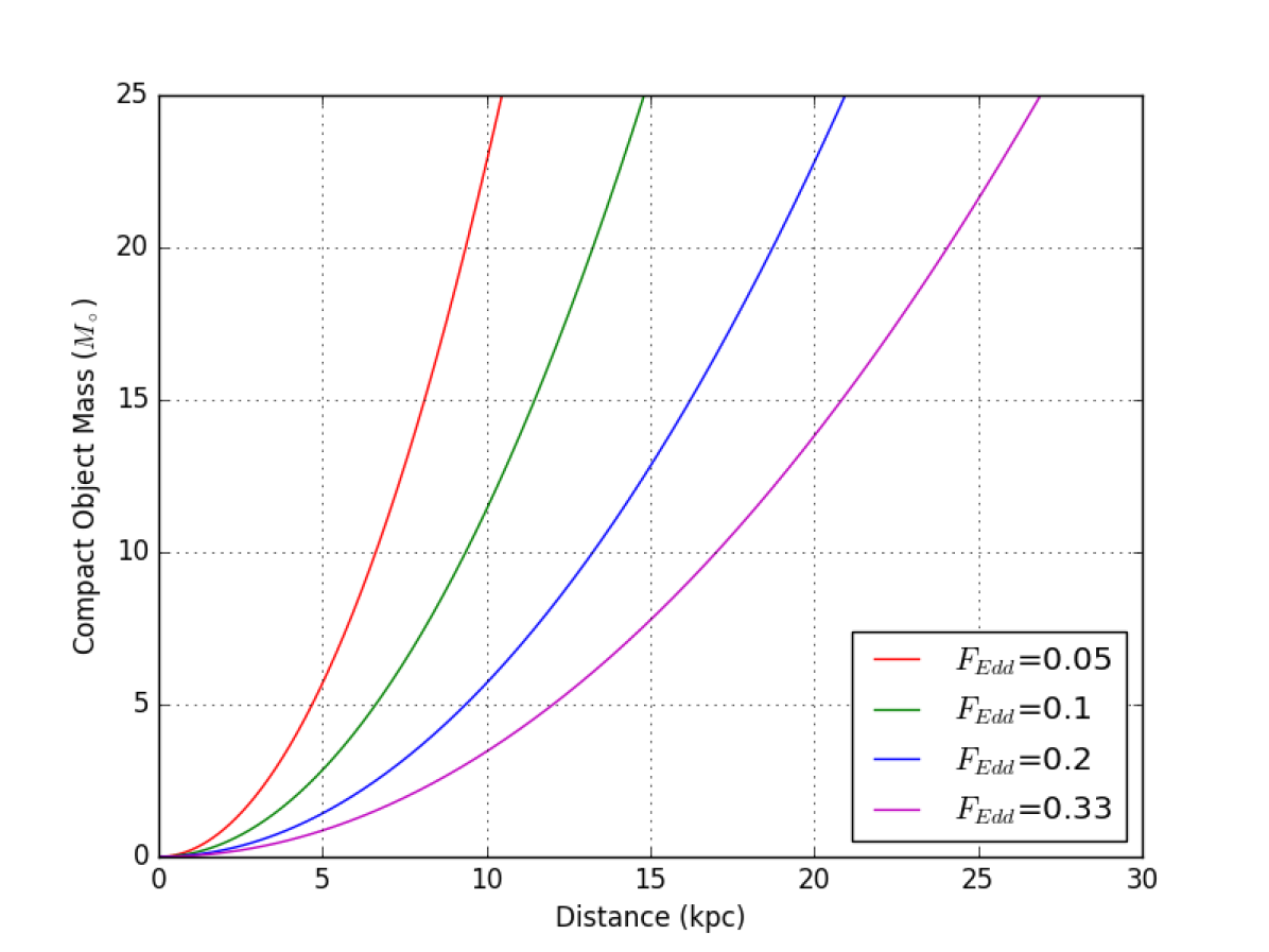
Figure 4.28: Mass of the compact object in IGR J17091-3624 plotted against its distance, for values of peak Eddington fractions of $F_{Edd}=$0.05, 0.1, 0.2 and 0.33.

4.3.6 Implications for Models of ‘Heartbeat’ Variability

I have found that hysteretic HID loops can execute in both directions in IGR J17091 (e.g. Section 4.3.4), as well as found a revised estimate that IGR J17091 accretes at $\lesssim 20$% Eddington (Section 4.3.5). Both of these findings have implications for physical models of GRS 1915-like variability in this source.

Firstly, I find that Eddington-limited accretion is neither necessary nor sufficient for GRS 1915-like variability. The discovery of GRS 1915-like variability in the sub-Eddington Rapid Burster (Bagnoli and in’t Zand,, 2015; Bagnoli et al.,, 2015) provided the first evidence that Eddington-limited accretion may not be a driving factor in this type of variability. I strengthen this case by finding that IGR J17091-3624 is also likely sub-Eddington. As such, I further rule out any scenario in which Eddington-limited accretion is required for GRS 1915-like variability in black hole LMXBs specifically.

Secondly, by using the direction of hysteretic HID loops, I find that hard photon lag in ‘heartbeat’-like classes of IGR J17091 can be either positive or negative. This could mean that we must rule out the causal connection between soft and hard emission being common to all classes.

In either case, I find that scenarios that require high global accretion rates or predict a consistent hard photon lag (e.g. Neilsen et al.,, 2011; Janiuk and Czerny,, 2005), are not able to explain GRS 1915-like variability in IGR J17091 unless they also feature geometric obscuration in a subset of variability classes. I note that simulations by Nayakshin et al.,, 2000 require an Eddington fraction of $\gtrsim 0.26$ before GRS 1915-like variability occurs, a value which falls in the range $\sim 0.05\mbox{--}0.33$ that I find for the peak Eddington fraction of IGR J17091.

An alternative way to explain the reversal of the direction of HID hysteresis is by considering the information propagation timescales in GRS 1915 and IGR J17091. A number of proposed models and scenarios to explain GRS 1915-like variability, such as the scenario of Neilsen et al., (2011) which we describe in Section 2.3.1, rely on information being propagated from one component of the LMXB system to another; in the scenario of Neilsen et al.,, this propagation takes the form of a disk wind which interacts with a geometrically displaced corona. Such a propagation takes a finite time. If the timescale of the propagation of information is similar to or greater than the characteristic timescale of heartbeat flares, then each hard pulse from the corona could take place immediately before the flare subsequent to the flare which triggered it. As heartbeats are a relatively coherent quasiperiodic phenomenon, it would appear to an observer that each hard pulse precedes a soft flare, even though in reality the causality is reversed. If this scenario was behind the hysteretic reversal seen in IGR J17091, then we would expect to see that only the fastest variability classes exhibited loops in the ‘wrong’ direction, indicating soft lags. However, I find that loops in Classes V, VI, VII and VIII in IGR J17091 show hard lags, whereas the slower classes III and IV show soft lags. Therefore I rule out an information propagation timescale-based explanation for the difference in HID hysteresis between IGR J17091 and GRS 1915.

In addition to being near its Eddington limit GRS 1915 also has the largest orbital period of any known LMXB (e.g. McClintock and Remillard,, 2006). Sa̧dowski,, 2016 have also shown that thin, radiation dominated regions of disks in LMXBs require a large-scale threaded magnetic field to be stable, and the field strength required to stabilise such a disk in GRS 1915 is higher than for any other LMXB they studied. I suggest that one of these parameters is more likely to be the criterion for GRS 1915-like variability. If better constraints can be placed on the disk size and minimum stabilising field strength in IGR J17091, it will become clear whether either of these parameters can be the unifying factor behind LMXBs that display GRS 1915-like variability.

4.4 Conclusions

I have constructed the first model-independent set of variability classes for the entire portion of the 2011–2013 outburst of IGR J17091 that was observed with RXTE. I find that the data are well-described by a set of 9 classes; 7 of these appear to have direct counterparts in GRS 1915, while two are, so far, unique to IGR J17091. D.A. and I find that variability in IGR J17091 is generally faster than in the corresponding classes of GRS 1915, and that patterns of quasi-periodic flares and dips form the basis of most variability in both objects. Despite this, I find evidence that ‘heartbeat’-like variability in both objects may be generated by different physical processes. In particular, while hard photons always lag soft in GRS 1915, I find evidence that hard photons can lag or precede soft photons in IGR J17091 depending on the variability class.

I also report on the long-term evolution of the 2011–2013 outburst of IGR J17091, in particular noting the presence of 3 re-flares during the later part of the outburst. Using an empirical relation between hard-soft transition luminosity and Eddington luminosity (Maccarone,, 2003), I estimate that IGR J17091 was likely accreting at no greater than $\sim 33$% of its Eddington limit at peak luminosity.

I use these results to conclude that any model of GRS 1915-like variability which requires a near-Eddington global accretion rate is insufficient to explain the variability we see in IGR J17091. As such I suggest that an extreme value of some different parameter, such as disk size or minimum stabilising large-scale magnetic field, may be the unifying factor behind all objects which display GRS 1915-like variability. This would explain why sub-Eddington sources such as IGR J17091 and the Rapid Burster do display GRS 1915-like variability, while other Eddington-limited sources such as GX 17+2 and V404 Cyg do not.

Chapter 5 The Evolution of X-ray Bursts in the ‘Bursting Pulsar’ GRO J1744–28

The fountains of the great deep came bursting through, and the windows of heaven were open.

Genesis 7:11

In Chapter 4, I present a new way to classify variability in the LMXB IGR J17091-3624. I compare this object with GRS 1915; although I find a number of differences between variability in the two systems, I conclude that the same broad phenomenon is likely behind variability in both. I also find that IGR J17091 is likely significantly sub-Eddington during periods in which it displays GRS 1915-like variability. This result can be seen as yet another piece of evidence that near-Eddington accretion is neither sufficient or necessary for GRS 1915-like behaviour.

To try and better constrain what does unite GRS 1915-like objects, the next step is to look for analogous behaviour in other systems. As previously mentioned, Bagnoli and in’t Zand, (2015) reported variability similar to GRS 1915 in RXTE lightcurves from the Rapid Burster. As such the Rapid Burster, and its sister system the Bursting Pulsar, are natural places to look for evidence of GRS 1915-like variability. Type II bursts seen in the Rapid Burster and the Bursting Pulsar are believed to be caused by viscous instabilities in the accretion disk (Lewin et al., 1976b, ), as is the X-ray variability seen GRS 1915 and IGR J17091. However, as I discuss in Section 2.4.1, the exact details of the mechanism responsible for Type II bursts remain unclear.

The Type II bursting behaviour in the Rapid Burster has been extensively studied (see e.g. Lewin et al., 1976b, ; Hoffman et al.,, 1978). Bagnoli et al., (2015) performed a full population study of all Type II bursts observed in this object by RXTE. Their results suggest that gating of the accretion by a strong magnetic field plays some role in the creation of Type II bursts: as this scenario requires a highly magnetised compact object, it cannot be employed to explain the variability seen in the black hole-primary GRS 1915 or IGR J17091. To further probe the physics behind Type II X-ray bursts, in this chapter I perform a similar population study on bursts from the Bursting Pulsar.

Previous work by Giles et al., (1996) indicated that Type II bursts in the 1995–1996 outburst of the Bursting Pulsar could be separated into a number of distinct populations based on peak flux. This is a notable difference from the Rapid Burster, in which all Type II bursts have peak fluxes approximately equal to or less than object’s Eddington Luminosity (Tan et al.,, 1991). In this chapter I expand on the work of Giles et al., (1996) and analyze RXTE, NuSTAR, Chandra, XMM-Newton, Swift and INTEGRAL data to fully quantify the population of Type II bursts in the Bursting Pulsar during all 3 outbursts in which they have been observed. I study how the bursting in this object evolves over time throughout each outburst, and I link this behaviour to the long-term evolution of the source. I also perform basic timing, morphology and spectral analysis on bursts, to try and understand the physical processes behind these phenomena.

The results I present in this chapter have been published as Court et al., 2018a .

5.1 Data and Data Analysis

Since discovery, the Bursting Pulsar has undergone three bright outbursts, which began in 1995, 1997 and 2014. I refer to these outbursts as Outbursts 1, 2 and 3. I do not consider the faint outburst in 2017 in this chapter (Sanna et al., 2017b, ), as no Type II bursts were observed during this time, nor do I analyse data taken while the source was in quiescence. See Daigne et al., (2002), Wijnands and Wang, (2002) and Degenaar et al., (2012) for studies of the Bursting Pulsar during quiescence.

I analysed data from all X-ray instruments which observed the Bursting Pulsar during these outbursts. Specifically, I analysed lightcurves, the evolution of hardness ratios as a function of time and of count rate, and performed statistical analysis of properties associated with each individual burst.

5.1.1 RXTE

I analysed data from RXTE/PCA corresponding to the Outbursts 1 & 2 of the Bursting Pulsar. This in turn corresponded to observation IDs starting with 10401-01, 20077-01, 20078-01, 20401-01 and 30075-01, between MJDs 50117 and 51225. This resulted in a total of 743 ks of data over 300 observations, which I have listed in Appendix B. Lightcurve data were extracted from fits files using FTOOLS. Errors were calculated and quoted at the 1$\,\sigma$ level.

I also use data from the RXTE/ASM to monitor the long-term evolution of the source. ASM data were taken from MIT’s ASM Light Curves Overview website.

Long-Term Evolution

To analyse the long-term evolution of the source during its outbursts, I extracted 2–16 keV count rates from the Standard2 PCA data in each observation. Following Altamirano et al., 2008b , I normalised the intensity estimated in each observation by the intensity of the Crab nebula, using the Crab observation that is the closest in time but within the same PCA gain epoch as the observation in question (see Jahoda et al.,, 2006).

Burst Identification and Analysis

To perform population studies on the Type II bursts in the Bursting Pulsar, I first extracted lightcurves from the Standard1 data in each observation, as this data is available for all RXTE/PCA observations. I used my own PANTHEON software to search these lightcurves and return a list of individual bursts, using the algorithm described in Section 3.2.1. I manually cleaned spurious detections from my sample. I defined a ‘burst’ as an event that lasted at least 3 seconds during which the 1 s binned count rate exceeded 3 standard deviations above the persistent emission level and reached a maximum of at least five standard devations above the persistent emission level. I did not subtract background, as all count rate-related parameters I analyse are persistent emission subtracted, automatically removing background contribution.

During the analysis, Arianna Albayati (A.A.) and I discovered a number of different burst ‘classes’, similar to the multiple classes of burst described by Giles et al., (1996). Our classes varied significantly in terms of overall structure, and as such needed to be treated separately; I show representative lightcurves from each of our classes in Figure 5.3. These classes were separated from one another by a number of criteria including peak count rate and recurrence time (the time between peaks of consecutive bursts).

The vast majority of detected bursts resembled the Type II bursts seen in the Rapid Burster (referred to as ‘Normal Bursts’ in Section 5.2) in terms of shape, duration and amplitude. I rebinned the data corresponding to these Normal Bursts to 0.5 s. I sampled the persistent emission before the burst, and defined the start of the burst as the first point at which count rate exceeded 5 standard deviations above the persistent emission before the burst. The end of the burst was defined similarly, but instead sampling the persistent emission after the burst; by doing this, I avoid making the implicit assumption that the persistent emission is equal before and after the burst. I fitted phenomenologically-motivated lightcurve models to each of these bursts (described in detail in Section 5.2.3), and used these fits to extract a number of parameters which characterise the shape and energetics of a burst (such as burst duration, total photon counts associated with a burst and persistent emission count rate).

Due to the high peak count rates of Normal Bursts, data were affected by dead-time (compare e.g. GRANAT data presented in Sazonov et al.,, 1997). I calculate the approximate Dead-Time Factors (DTFs) for a number of the brightest Normal Bursts in my sample, using 1 s binned data, using the following formula in the RXTE Cookbook:

$$\Delta=\frac{C_{Xe}+C_{Vp}+C_{Rc}+15C_{VL}}{N_{PCU}}\times 10^{-5}$$ (5.1)

Where $\Delta$ is the fractional detector deadtime, $C_{Xe}$ is the Good Xenon count rate, $C_{Vp}$ is the coincident event count rate, $C_{Rc}$ is the propane layer count rate, $C_{VL}$ is the very large event count rate and $N_{PCU}$ is the number of PCUs active at the time.

I estimate that dead-time effects reduce the peak count rates of Normal Bursts by no more than $\sim 12$%; however, due to the sharply-peaked nature of bursts from the Bursting Pulsar, the deadtime effect depends on the binning used. Due to this ambiguity I do not correct for dead-time in Normal Bursts. The dead-time corrections required for the count rates seen in other classes of burst are minimal, as they are orders of magnitude fainter (Giles et al.,, 1996).

To test for correlations between parameters in a model-independent way, I used the Spearman’s Rank correlation coefficient (as available in Scipy, Jones et al.,, 2001). This metric only tests the hypothesis that an increase in the value of one parameter is likely to correspond to an increase in the value of another parameter, and it is not affected by the shape of the monotonic correlation to be measured. Although dead-time effects lead to artificially low count rates being reported, a higher intensity still corresponds to a higher reported count rate. As such, using this correlation coefficient removed the effects of dead-time on my detection of any correlations.

To calculate the distribution of recurrence times between consecutive bursts, I considered observations containing multiple bursts. If fewer than 25 s of data gap exists between a pair of bursts, I considered them to be consecutive and added their recurrence time to the distribution. I choose this maximum gap size as this is approximately the timescale over which a Normal Burst occurs.

When SB_62us_0_23_500ms and SB_62us_24_249_500ms data were available, I divided my data into two energy bands: A (PCA channels 0–23, corresponding to $\sim 2$–$7$ keV) and B (channels 24–249, corresponding to $\sim 8$–$60$ keV). The evolution of colour (defined as the ratio of the count rates in B and A) throughout a burst could then be studied. Due to the very high count rates during Normal Bursts, I did not correct for background. During fainter types of burst I estimate the background in different energy bands by subtracting count rates from RXTE observation 30075-01-26-00 of this region, when the source was in quiescence. Unlike using the RXTE background model, this method subtracts the contributions from other sources in the field. However, as it is unclear whether any of the rest of these sources are variable, the absolute values of colours I quote should be treated with caution. I created hardness-intensity diagrams to search for evidence of hysteretic loops in hardness-intensity space.

Following Bagnoli et al., (2015), I used the total number of persistent emission-subtracted counts as a proxy for fluence for all bursts other than Normal Bursts. As the contribution of the background does not change much during a single observation, this method also automatically subtracts background counts from my results.

Detecting Pulsations

The Bursting Pulsar is situated in a very dense region of the sky close to the Galactic centre, and so several additional objects also fall within the 1^∘ RXTE/PCA field of view. Therefore it is important to confirm that the variability I observe in my data does in fact originate from the Bursting Pulsar.

To ascertain that all bursts considered in this study are from the Bursting Pulsar, Dr. Andrea Sanna (A.S.) analysed the coherent X-ray pulse at the pulsar spin frequency to confirm that the source was active. A.S. first corrected the photon time of arrivals of the RXTE/PCA dataset, and barycentred this data using the faxbary tool available in FTOOLS (DE-405 Solar System ephemeris). A.S. corrected for the binary motion by using the orbital parameters reported by Finger et al., 1996a .

For each  PCA observation A.S. investigated the presence of the $\sim 2.14$ Hz coherent pulsation by performing an epoch-folding search of the data using 16 phase bins and starting with the spin frequency value $\nu=2.141004$ Hz, corresponding to the spin frequency measured from the 1996 outburst of the source (Finger et al., 1996a, ), with a frequency step of $10^{-5}$ Hz for 10001 total steps. A.S. detected X-ray coherent pulsations in all PCA observations performed during Outbursts 1 & 2.

5.1.2 Swift

In this study, I made use of data from  XRT and  BAT aboard Swift. I extracted a long-term 0.3–10 keV Swift/XRT lightcurve of Outburst 3 using the lightcurve generator provided by the UK Swift Science Data Centre (UKSSDC, Evans et al.,, 2007). I also make use of Swift/BAT lightcurves from the Swift/BAT Hard X-ray Transient website (see Krimm et al.,, 2013).

5.1.3 INTEGRAL

I also made use of data from IBIS aboard INTEGRAL. I extracted 17.3–80 keV IBIS/ISGRI lightcurves of the Bursting Pulsar during Outburst 3 using the INTEGRAL Heavens portal. This is provided by the INTEGRAL Science Data Centre (Lubiński,, 2009).

5.1.4 Chandra

The Bursting Pulsar was targeted with Chandra three times during Outburst 3 (Table 5.1). One of these observations (OBSID 16596) was taken simultaneously with a NuSTAR observation (80002017004). In all three observations data were obtained with the HETG, where the incoming light was dispersed onto the  ACIS-S array. The ACIS-S was operated in continued clocking (CC) mode to minimize the effects of pile-up. The Chandra/HETG observations were analysed using standard tools available within ciao v. 4.5 (Fruscione et al.,, 2006). Dr. Nathalie Degenaar (N.D.) extracted 1 s binned lightcurves from the evt2 data using dmextract, where the first order positive and negative grating data from both the Medium Energy Grating (MEG; 0.4-5 keV) and the High Energy Grating (HEG; 0.8–8 keV) were combined.

OBSID	Exposure (ks)	MJD	Reference
16596	10	56719	Younes et al., (2015)
16605	35	56745	Degenaar et al., 2014a
16606	35	56747	Degenaar et al., 2014a

Table 5.1: Information on the three Chandra observations of the Bursting Pulsar during Outburst 3. All other observations of the Bursting Pulsar in the Chandra archive were obtained at times that the source was in quiescence.

5.1.5 XMM-Newton

A single pointed XMM-Newton observation of the Bursting Pulsar was taken during Outburst 3 on MJD 56722 (OBSID 0729560401) for 85 ks. I extracted a 0.5–10 keV lightcurve from EPIC-PN at 1 s resolution using SAS version 15.0.0. During this observation, EPIC-PN was operating in Fast Timing mode. I use EPIC-PN as the statistics are better than in MOS1 or MOS2.

5.1.6 Suzaku

Suzaku observed the Bursting Pulsar once during Outburst 3 on MJD 56740 (OBSID 908004010). To create a lightcurve, K.Y. reprocessed and screened data from the X-ray Imaging Spectrometer (XIS, Koyama et al.,, 2007) using the aepipeline script and the latest calibration database released on June 7, 2016. The attitude correction for the thermal wobbling was made by aeattcor2 and xiscoord (Uchiyama et al.,, 2008). The source was extracted within a radius of 250 pixels corresponding to 260” from the image center. The background was extracted from two regions near either end of the XIS chip, and subtracted from the source.

5.1.7 NuSTAR

NuSTAR observed the Bursting Pulsar three times during its outbursts, all times in Outburst 3. One of these observations was taken while the Bursting Pulsar was not showing X-ray bursts, and the other two are shown in Table 5.2. I extracted lightcurves from both of these observations using nupipeline and nuproducts, following standard procedures.

OBSID	Exposure (ks)	MJD	Reference
80002017002	29	56703	D’Aì et al., (2016)
80002017004	9	56719	Younes et al., (2015)

Table 5.2: Information on the two NuSTAR observations of the Bursting Pulsar during the main part of Outburst 3.

5.2 Results

5.2.1 Outburst Evolution

I show the long-term monitoring lightcurves of Outbursts 1, 2 and 3 in Figure 5.1, as well as mark the dates of pointed observations with various instruments.

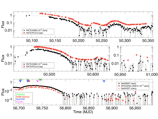
Figure 5.1: Comparisons of the three outbursts of the Bursting Pulsar reported on in this chapter. Times corresponding to pointed observations with Chandra, NuSTAR, Suzaku, Swift and XMM-Newton are marked.

The Bursting Pulsar was discovered already in outburst on December 12 1995 (Fishman et al.,, 1995); CGRO/BATSE data suggest that this outburst began several days earlier on December 3 (Paciesas et al.,, 1996; Bildsten et al.,, 1997). The main outburst ended around May 10 1996 (Woods et al.,, 2000). I show the global lightcurve of this outburst in Figure 5.1, Panel 1. As RXTE did not observe the object before or during the peak of Outburst, I can only obtain a lower limit of $\sim 1.75$ Crab for the peak 2–16 keV flux.

There are at least two major rebrightening events in the tail of Outburst 1, which can be seen clearly in Figure 5.1 centred at MJDs of $\sim 50235$ and $\sim 50280$. During these rebrightening events, the 2–16 keV flux peaked at $\sim 0.10$ and $\sim 0.18$ Crab respectively.

Outburst 2 began on December 1 1996 and ended around April 7 1997 (Woods et al.,, 1999). The 2–16 keV flux peaked at 1.02 Crab on MJD 50473; I show the global lightcurve of this outburst in Figure 5.1, Panel 2. Type II-like bursts are seen in RXTE/PCA lightcurves from Outburst 2 between MJDs 50466 and 50544. One rebrightening event occurred during the tail of Outburst 2, centred at an MJD of $\sim 50615$ with a peak 2–16 keV flux of $\sim 54$ mCrab. A second possible rebrightening event occurs at MJD 50975, with a peak 2–16 keV flux of 11 mCrab, but the cadence of RXTE/PCA observations was too low to unambiguously confirm the existence of a re-flare at this time.

Outburst 3 began on January 31, 2014 (Negoro et al.,, 2014; Kennea et al.,, 2014) and ended around April 23 (e.g. D’Aì et al.,, 2015). The daily 0.3–10 keV Swift/XRT rate peaked at 81 cts s^-1 on MJD 56729, corresponding to 0.4 Crab. I show the global lightcurve of this outburst in Figure 5.1, Panel 3.

During the main part of Outburst 3, Swift, XMM-Newton and Suzaku made one pointed observation each, Chandra made four observations, and NuSTAR made three observations. The Chandra observation on March 3 2014 was made simultaneously with one of the NuSTAR observations (see Younes et al.,, 2015). After the main part of the outburst, the source was not well-monitored, although it remained detectable by Swift/BAT, and it is unclear whether any rebrightening events occured. A single NuSTAR observation was made during the outburst tail on August 14 2014.

As can be seen in Figure 5.1, the main section of all three outbursts follow a common profile, over a timescale of $\sim 150$ days. A notable difference between outbursts 1 & 2 is the number of rebrightening events; while I find two re-flares associated with Outburst 1, I only find one associated with Outburst 2 unless I assume the event at MJD 50975 is associated with the outburst. Additionally, Outburst 2 was at least a factor $\sim 1.7$ fainter at its peak than Outburst 1 (see also Woods et al.,, 1999), while Outburst 3 was a factor of $\gtrsim 4$ fainter at peak than Outburst 1.

Pulsations

A.S. found pulsations in PCA data throughout the entirety of Outbursts 1 & 2. This confirms that the Bursting Pulsar was active as an X-ray pulsar in all of my observations, leading us to conclude that all the types of X-ray burst that we see are from the Bursting Pulsar. In Figure 5.2, I show that the amplitude of these pulsations approximately followed the intensity of the source in both outbursts, but there were significant deviations from this trend. These deviations will require further investigation, and a comparison with other accreting pulsar systems. Previous studies have shown that pulsations were also present during Outburst 3 (e.g. Sanna et al., 2017c, ).

Figure 5.2: 2–16 keV RXTE/PCA lightcurves of Outbursts 1 & 2 of the Bursting Pulsar (solid blue), overlaid with plots showing how the fractional RMS of the 2.4 Hz pulsation associated with the pulsar changes as a function of time during these outbursts (orange crosses).

Bursting Behaviour

Bursts are seen in RXTE/PCA lightcurves from the start of the Outburst 1 (e.g. Kouveliotou et al., 1996b, ). These bursts occur until around MJD 50200, as the source flux falls below $\sim 0.1$ Crab in the 2–16 keV band.

During the latter part of the first rebrightening after Outburst 1, between MJDs 50238 and 50246, A.A. found Type II-like bursts with amplitudes $\sim 2$ orders of magnitude smaller than those found during the main outburst event. These gradually increased in frequency throughout this period of time until evolving into a period of highly structured variability which persisted until MJD 50261.

In Outburst 2, Type II bursts occured between MJDs $\sim 50466$ and $50542$. Low-amplitude Type II-like bursts were seen during the latter stages of the main outburst, between MJDs 50562 and 50577. These again evolved into a period of highly structured variability; this persisted until MJD 50618, just after the peak of the rebrightening event.

High-amplitude Type II bursts were also seen in Outburst 3 (e.g. Linares et al.,, 2014). As no soft ($\lesssim 10\,$keV) X-ray instrument was monitoring the Bursting Pulsar during the latter part of Outburst 3, it is unknown whether this Outburst showed the lower-amplitude bursting behaviour seen at the end of Outbursts 1 & 2. Low amplitude bursting behaviour is not seen in the pointed NuSTAR observation which was made during this time.

5.2.2 Categorizing Bursts

A.A. and I found that bursts in the Bursting Pulsar fall into a number of discrete classes, lightcurves from which I show in Figure 5.3. These classes are as follows:

Figure 5.3: 2–49 keV lightcurves for the four classes of bursting behaviour identified in this chapter: a) Normal Burst, b) Miniburst, c) Mesoburst, d) Structured Bursts. Note that Panel d is plotted with a different time scaling to the other panels so as to better show the behaviour of Structured Bursting. On all figures the median count rate, which I use as a proxy for the persistent emission, is plotted in cyan. Lightcurves a-c are binned to 0.125 s, while lightcurve d is binned to 1 s.

• Normal Bursts (Figure 5.3, Panel a): the brightest bursts seen from this source, with peak count 1 s binned rates of $\sim 10000$ cts s^-1 PCU^-1, and recurrence timescales of order $\sim 1000$ s. These bursts are roughly Gaussian in shape with durations of $\sim 10$ s, and are followed by a ‘dip’ in the persistent emission count rate with a duration of order 100 s (see also e.g. Giles et al.,, 1996).

• Minibursts (Figure 5.3, Panel b): faint bursts with 1 s-binned peak count rates of $\sim 2$ times the persistent emission count rate. Minibursts are variable, with duration timescales between $\sim 5$–50 s. These bursts are also sometimes followed by dips similar to those seen after Normal Bursts.

• Mesobursts (Figure 5.3, Panel c): Type II-like bursts. These bursts differ from Normal Bursts in that they do not show well-defined subsequent ‘dips’. They are also fainter than Normal Bursts, with peak count 1 s binned count rates of $\sim 1000$ cts s^-1 PCU^-1. Their burst profiles show fast rises on timescales of seconds, with slower decays and overall durations of $\sim 50$ s. The structure of the bursts is very non-Gaussian, appearing as a small forest of peaks in lightcurves.

• Structured Bursts (Figure 5.3, Panel d): the most complex class of bursting behaviour we observe from the Bursting Pulsar, consisting of patterns of flares and dips in the X-ray lightcurve. The amplitudes of individual flares are similar to those of the faintest Mesobursts. The recurrence timescale is of the order of the timescale of an individual flare, meaning that is it difficult to fully separate individual flares of this class.

In the upper panel of Figure 5.4 I show a histogram of persistent-emission-subtracted peak count rates for all Normal and Mesobursts observed by RXTE. I split these two classes based on the bimodal distribution in peak count rate as well as the lack of dips in Mesobursts. In the lower panel of Figure 5.4, I show the histogram of peak count rates for all Normal and Minibursts observed by RXTE as a fraction of the persistent emission at that time. I split these two classes based on the strongly bimodal distribution in fractional amplitude.

Figure 5.4: Upper Panel: A histogram of the peak 1 s binned peak count rates of the joint population of all Normal and Mesobursts seen by RXTE. The dashed line indicates the position of the threshold above which I consider a Type II-like burst to be a Normal Burst. The resultant split of the population into Normal and Mesobursts is indicated by blue and red shading respectively. The skewed shape of the distribution of Normal Bursts is due to the effects of dead-time putting an effective cap on their maximum observed intensity. Lower Panel: A histogram of the peak 1 s binned peak count rates of the joint population of all Normal and Minibursts seen by RXTE, divided by the persistent emission count rate at that time. The dashed line indicates the position of the threshold below which I consider a burst to be a Miniburst. The resultant split of the population into Normal and Minibursts is indicated by blue and green shading respectively. Note that the $x$-axis of both plots is logarithmic, and so number density is not preserved.

I also find 6 bursts with fast ($\sim 1$ s) rises and exponential decays that occur during the lowest flux regions of the outburst ($\lesssim 50$ mCrab). Strohmayer et al., (1997) and Galloway et al., (2008) have previously identified these bursts as being Type I X-ray bursts from another source in the RXTE field of view. To show that these unrelated Type I bursts would not be confused with Minibursts, I add examples of the Type I bursts to lightcurves from observations containing Minibursts. I find that the peak count rates in Type I bursts are roughly equal to the amplitude of the noise in the persistent flux in these observations, hence they would not be detected by my algorithms.

I show when in Outbursts 1 & 2 each type of burst was observed in Figures 5.5 and 5.6 respectively. Normal Bursts and Minibursts (red) occur during the same periods of time from around the peak of an outburst until the persistent emission falls beneath $\sim 0.1$ Crab; assuming an Eddington Limit of $\sim 1$ Crab (e.g Sazonov et al.,, 1997), this corresponds to an Eddington ratio of $\sim 0.1$. After this point, bursting is not observed for a few tens of days. Mesobursts (blue) begin at the end of a rebrightening event in Outburst 1 and during the final days of the main part of the outburst in Outburst 2. Structured Bursts (yellow) occur during the first part of a rebrightening event in both outbursts. Although there was a second rebrightening event after Outburst 1, neither Mesobursts nor Structured Bursts were observed at this time. Based on this separation, as well as differences in structure, I treat each class of burst separately below.

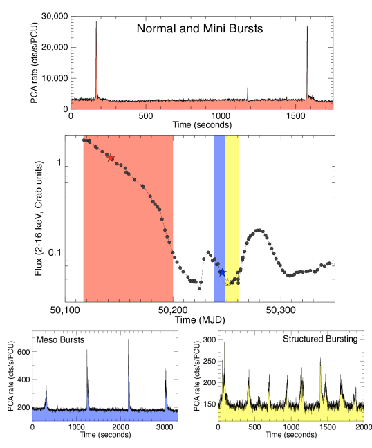
Figure 5.5: Central panel shows the global 2–16 keV RXTE/PCA lightcurve of the 1995–1996 outburst of the Bursting Pulsar, highlighting periods of time during which Mesobursts (blue) Structured Bursts (yellow) or Normal and Mini bursts (red) are observed. A single Mesoburst was also observed on MJD 50253, during the period of the outburst highlighted in yellow (see Figure 5.18). Other panels show example lightcurves which contain the aforementioned types of bursting behaviour. See section 5.2.2 for a detailed treatment of burst classification. Fluxes reported in units of Crab.

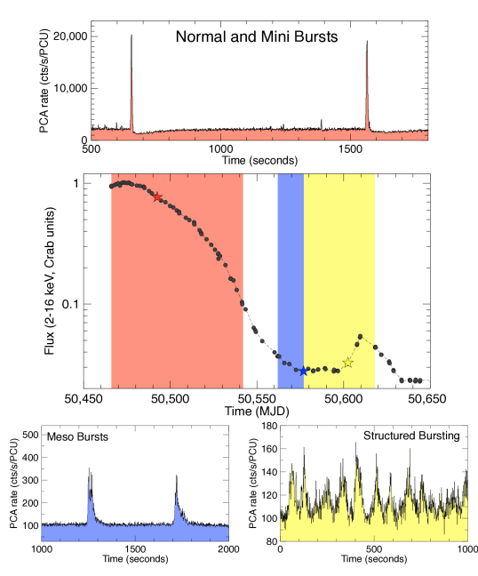
Figure 5.6: Central panel shows the global 2–16 keV RXTE/PCA lightcurve of the 1997–1999 outburst of the Bursting Pulsar, highlighting periods of time during which Mesobursts (blue) Structured Bursts (yellow) or Normal and Mini bursts (red) are observed. Other panels show example lightcurves which contain the aforementioned types of bursting behaviour.

5.2.3 Normal Bursts

I define Normal Bursts as the set of all bursts with a persistent-emission-subtracted peak 1 s binned RXTE/PCA-equivalent count rate above 3000 cts s^-1 PCU^-1. Normal Bursts account for 99 out of the 190 bursts identified for this study. They are observed during all three outbursts covered in this study. They occurred between MJDs 50117 and 50200 in Outburst 1, and between 50466 and 50542 in Outburst 2; during these intervals, RXTE observed the source for a total of 192 ks. See Table 5.3 to compare these with numbers for the other classes of burst identified in this study. Normal Bursts occur during the same time intervals in which Minibursts are present. In both of these outbursts, the period of Normal and Minibursts correspond to the time between the peak of the outburst and and the time that the persistent intensity falls below $\sim 0.1$ Crab.

Bursting Mode	Bursts	Total Exposure (ks)	Duration (d)
Normal Bursts	99	192	76
Minibursts	48	192	76
Mesobursts	43	44	25
Structured Bursts	-	80	54

Table 5.3: Statistics on the population of bursts I use for this study, as well as the duration and integrated RXTE/PCA exposure time of each mode of bursting. All numbers are the sum of values for Outbursts 1 and 2. As Normal and Minibursts happen during the same period of time in each outburst, the exposure time and mode duration for these classes of bursting are equal.

Recurrence Time

Using Outburst 3 data from Chandra, XMM-Newton, NuSTAR and Suzaku, I find minimum and maximum Normal Burst recurrence times of $\sim 345$ and $\sim 5660$ s respectively. I show the histogram of recurrence times from Outburst 3 in Figure 5.7, showing which parts of the distribution were observed with which observatory. Compared to data from Chandra and XMM-Newton, data from Suzaku generally suggests shorter recurrence times. This is likely due to Suzaku observations consisting of a number of $\sim 2$ ks windows; as this number is of the same order of magnitude as the recurrence time between bursts, there is a strong selection effect against high recurrence times in the Suzaku dataset.

From the RXTE data I find minimum and maximum Normal Burst recurrence times of $\sim 250$ and $\sim 2510$ s during Outburst 1, and minimum and maximum recurrence times of $\sim 250$ and $\sim 2340$ s during Outburst 2. As the length of an RXTE pointing ($\lesssim 3$ ks) is also of the same order of magnitude as the recurrence time between bursts, selection effects bias us against sampling pairs of bursts with longer recurrence times, and hence this upper value is likely an underestimate.

Figure 5.7: The distribution of recurrence times between consecutive Normal Bursts seen in pointed Chandra, XMM-Newton, NuSTAR and Suzaku observations of Outburst 3 of the Bursting Pulsar. Distributions of bursts observed by different instruments are stacked on top of each other and colour coded.

To test whether consecutive Normal Bursts are independent events, I tested the hypothesis that bursts are randomly distributed in time in a Poisson distribution (Poisson,, 1837). Assuming my hypothesis, as well as assuming that the frequency of Normal Bursts does not change during an outburst (e.g. Aptekar et al.,, 1998), I could concatenate different observations and the resultant distribution of burst times should still be Poissonian. For each of Outbursts 1 & 2, I concatenated all RXTE data during the Normal Bursting part of the outburst into a single lightcurve. I split this concatenated lightcurve into windows of length $w$ and counted how many bursts were in each, forming a histogram of number of bursts per window for the combined set of all bursts. I fit this histogram with a Poisson probability density function, obtaining the value $\lambda$ which is the mean number of bursts in a time $w$. $\lambda/w$ is therefore an expression of the true burst frequency per unit time, and should be independent of my choice of $w$. I tried values of $w$ between 100 and 10000 s for both outbursts, and found that in all cases $\lambda/w$ depends strongly on $w$. Therefore my assumptions cannot both be valid, and I rejected the hypothesis that these bursts are from a Poisson distribution with constant $\lambda$. This in turn suggests at least one of the following must be correct:

1. The average recurrence time of bursts was not constant throughout the outburst. Or:

2. The arrival time of a given burst depends on the arrival time of the preceding burst, and therefore bursts are not independent events.

Burst Structure

In the top panel of Figure 5.8 I show a plot of all Normal Bursts observed with RXTE overlayed on top of one another. I find that all Normal Bursts follow a similar burst profile with similar rise and decay timescales but varying peak intensities. In the lower panel of Figure 5.8 I show a plot of Normal Bursts overlaid on top of each other after being normalised by the persistent emission count rate in their respective observation. The bursts are even closer to following a single profile in this figure, suggesting a correlation between persistent emission level in an outburst and the individual fluence of its bursts.

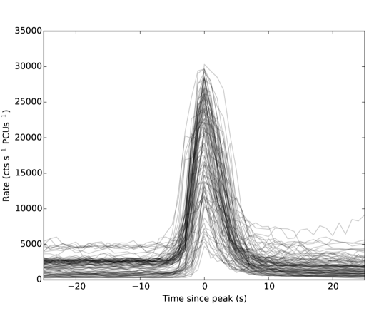
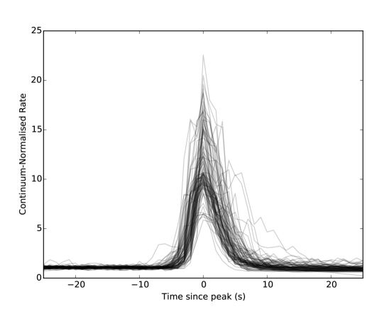
Figure 5.8: Top: a lightcurve of every Normal Burst, centred by the time of its peak, overlaid on top of each other to show the existence of a common pulse profile. Bottom: a lightcurve of every Normal Burst in which count rates have been normalised by the persistent emission count rate during the observation from which each burst was observed. As the bursts are on average closer to the average pulse profile in this metric, this suggests that the intensity of a burst is roughly dependent on the persistent emission rate. Some persistent emission-normalised count rates may be artificially low due to dead-time effects.

The structure of the lightcurve of a Normal Burst can be described in three well-defined parts:

1. The main burst: roughly approximated by a skewed Gaussian (see e.g. Azzalini,, 1985).

2. A ‘plateau’: a period of time after the main burst during which count rate remains relatively stable at a level above the pre-burst rate.

3. A ‘dip’: a period during which the count rate falls below the persistent level, before exponentially decaying back up towards the pre-burst level (e.g. Younes et al.,, 2015).

The dip is present after every Normal Burst in my RXTE sample from Outbursts 1 & 2, whereas the plateau is only seen in 39 out of 99. I show example lightcurves of bursts with and without plateaus in Figure 5.9, which also show that the dip is present in both cases.

Figure 5.9: RXTE lightcurves of Normal Bursts with (top) and without (bottom) ‘plateau’ features, showing the burst structure in each case. The median count rate, which I use as a proxy for the persistent emission, is plotted in cyan to highlight the presence of the count rate ‘dip’ after each burst.

In order to study Normal Bursts, I fit the burst profiles with phenomenologically-motivated mathematical functions. In Figure 5.10 I show a schematic plot of my model, as well as annotations explaining the identities of the various parameters I use. I fit the main burst with a skewed Gaussian, centred at $t=x_{0}$ with amplitude $a_{b}$, standard deviation $\sigma_{B}$ and skewness $c$, added to the persistent emission rate $k$. I fit the ‘dip’ with the continuous piecewise function ‘Dipper function’ $f(t)$:

$$f(t)=\begin{dcases}k-\frac{a_{d}(t-t_{0})}{d-t_{0}},&\text{if }t\leq d\\ k-a_{d}\exp\left(\frac{d-t}{\lambda}\right),&\text{otherwise}\end{dcases}$$ (5.2)

Where $t$ is time, $t_{0}$ is the start time of the dip, $a_{d}$ is the amplitude of the dip, $d$ is the time at the local dip minimum and $\lambda$ is the dip recovery timescale. This function is based on the finding by Younes et al., (2015) that dip count rates recover exponentially, but has the added advantage that the start of the recovery phase can also be fit as an independent parameter. Using this fit, I can estimate values for burst fluence $\phi_{B}$, burst scale-length $\sigma_{B}$, ‘missing’ dip fluence $\phi_{D}$ and dip scale-length $\lambda$ and compare these with other burst parameters. When present, I also calculate the fluence of the plateau $\phi_{p}$ by summing the persistent emission-subtracted counts during the region between the end of the burst (as defined in Section 5.1.1) and the start of the dip. For each pair of parameters, I do not consider datapoints when the magnitude of the error on a parameter is greater than the value of the parameter.

Figure 5.10: A schematic explaining the origin of the 12 Normal Burst parameters used in this study, as well as showing the functional forms of both the skewed Gaussian fit to a burst and the ‘dipper function’ (Equation 5.2) fit to a dip. Note that I do not fit a function to the plateau, and I calculate its fluence by summing the persistent rate-subtracted counts. Diagram is for explanation only and the burst pictured is neither based on real data nor to scale.

I only extract these parameters from Normal Bursts observed by RXTE during Outbursts 1 & 2. This ensures that the resultant parameter distributions I extracted are not affected by differences between instruments.

Parameter Distributions

I extracted a total of ten parameters from my fit to each burst: the parameters $a_{d}$, $d$ and $\lambda$ of the fit to the dip, the missing fluence $\phi_{D}$ of the dip, the parameters $a_{b}$, $\sigma_{B}$ and $c$ of the skewed Gaussian fit to the main burst, the main burst fluence $\phi_{B}$, the maximum persistent emission-subtracted rate in the plateau $a_{p}$ and the plateau fluence $\phi_{P}$.

Using my RXTE sample of Normal Bursts, I can construct distributions for all of the burst parameters described in Section 5.2.3 for bursts in Outbursts 1 & 2. I give the mean and standard deviation for each parameter in each outburst in Table 5.4, and histograms for each can be found in Appendix C.

	Outburst 1		Outburst 2		Outbursts 1&2
	Mean	S.D.	Mean	S.D.	Mean	S.D.
$\phi_{B}$	2.74e6	7.8e5	2.25e6	7.6e5	$2.43\mathrm{e}6$	$8.0\mathrm{e}5$
$a_{B}$	3.18e5	8.4e4	2.72e5	9.9e4	$2.90\mathrm{e}5$	$9.6\mathrm{e}4$
$\sigma_{B}$	3.39	0.35	3.42	0.59	3.41	0.52
$c$	2.68	1.9	2.79	2.0	2.75	2.0
$\phi_{d}$	1.74e6	1.3e6	1.17e6	3.6e5	$1.38\mathrm{e}6$	$8.7\mathrm{e}5$
$a_{d}$	550	335	536	307	541	318
$d$	49	46	20	22	31	36
$\lambda$	294	176	229	124	254	150
$\phi_{p}$	1.89e5	2.3e5	7577	5707	1.4e5	1.8e5
$a_{p}$	1289	1113	767	463	1063	928

Table 5.4: A table showing the mean and standard deviation of 10 Normal Burst parameters of RXTE-sampled bursts. In each case, I give the values for populations from only Outburst 1, from only Outburst 2 and from the combined population from both outbursts. Histograms for each parameter can be found in Appendix C.

The mean value of most parameters differs by no more than $\sim 50$% between outbursts. Notable exceptions are $d$, $\phi_{p}$, $\phi_{d}$ and $a_{p}$, which are $\sim 2.5$, $\sim 2.5$ $\sim 1.5$ and $\sim 1.7$ times greater in Outburst 1 than in Outburst 2 respectively. The less significant differences between values of $\phi_{B}$ and $a_{B}$ in Outbursts 1 & 2 are expected, as the amplitude of a burst correlates with persistent rate $k$ which was generally higher in Outburst 1 than in Outburst 2.

Correlations

In total, I extracted 12 parameters for each Normal Burst in my RXTE sample: the 10 burst parameters listed in Section 5.2.3, the recurrence time $s_{t}$ until the next burst and the persistent emission rate $k$ at the time of the burst.

As the amplitude of all 3 components in a burst scale with the persistent emission level, I rescaled my values of $a_{b}$, $a_{d}$, $\phi_{B}$, $\phi_{D}$ and $\phi_{P}$ by a factor $\frac{1}{k}$. I show the covariance matrix with all 66 possible pairings of these normalised parameters in Figure 5.11 (we present the covariance matrix of these parameters before being rescaled in Appendix LABEL:app:corr). Using the Spearman’s Rank Correlation Coefficient, I find the following $\geq 5\,\sigma$ correlations which are highlighted in Figure 5.11:

• Persistent emission $k$ anticorrelates with normalised burst fluence $\phi_{B}/k$ ($>10\,\sigma$) and normalised burst amplitude $a_{b}/k$ ($>10\,\sigma$).

• Normalised burst fluence $\phi_{B}/k$ correlates with normalised burst amplitude $a_{B}/k$ ($8.0\,\sigma$).

• Normalised dip fluence $\phi_{d}/k$ correlates with dip recovery timescale $\lambda$ ($6.3\,\sigma$).

• Normalised dip amplitude $a_{d}/k$ anticorrelates with dip falltime $d$ ($5.7\,\sigma$) and dip recovery timescale $\lambda$ ($7.1\,\sigma$).

• Normalised plateau fluence $\phi_{p}/k$ correlates with normalised plateau amplitude $a_{p}$ ($6.4\,\sigma$).

As $\phi_{B}$ can be approximated to first order as a product of $a_{B}$ and $\sigma$, the correlation between $\phi_{B}$ and $a_{B}$ is expected as they are not independent parameters. Similarly, the correlations between $\phi_{d}$ & $\lambda$ and $\phi_{p}$ and $a_{p}$ are likely due to these pairs of parameters not being independent.

Figure 5.11: Covariance Matrix with a scatter plot of each of the 66 pairings of the 12 Normal Burst parameters listed in section 5.2.3. Amplitudes and fluences have been normalised by dividing by the persistent emission rate $k$. Pairings which show a correlation using the Spearman Rank metric with a significance $\geq 5\,\sigma$ are highlighted in red.

Colour Evolution

To explore the spectral behaviour of Normal Bursts, Toyah Overton (T.O.) and I studied the evolution of the hardness (the ratio between count rate in the energy bands $\sim 2$–$7$ and $\sim 8$–$60$ keV energy bands) as a function of count rate during the individual bursts. Plotting hardness-intensity diagrams allow us to check for spectral evolution in a model-independent way. We do not correct them for background as the count rates in both bands are very high.

T.O. and I find evidence of hysteretic loops in hardness-intensity space in some, but not all, of the Normal Bursts in my sample; see Figure 5.12 for an example of such a loop. The existence of such a loop suggests significant spectral evolution throughout the burst. This finding can be contrasted with results from previous studies in different energy bands (e.g. Woods et al.,, 1999 from $\sim 25$–100 keV) which suggested no spectral evolution during Type II bursts in this source.

Figure 5.12: A 1 s-binned hardness-intensity diagram of a Normal Burst from RXTE/PCA observation 10401-01-08-00, with an inset 2–60 keV lightcurve. Significant colour evolution can be seen during the burst, taking the form of a loop.

5.2.4 Minibursts

I define Minibursts as the set of all bursts with a peak 1 s binned RXTE/PCA-equivalent count rate of $<300\%$ of the persistent rate. Minibursts account for 48 out of the 190 bursts identified for this study. They are observed during all 3 Outbursts, and occur during the same times that Normal Bursts are present. Minibursts occurred between MJDs 50117 and 50200 in Outburst 1, and between 50466 and 50542 in Outburst 2; during these intervals, RXTE observed the source for a total of 192 ks. These intervals correspond to the times between the peak of each outburst and and the time that the persistent intensity falls below $\sim 0.1$ Crab.

Recurrence Time

There are only 10 observations with RXTE which contain multiple Minibursts. Using these, I find minimum and maximum Miniburst recurrence times of 116 and 1230 s.

I find 17 RXTE observations which contain both a Miniburst and a preceding Normal Burst, and find minimum and maximum Normal Burst $\rightarrow$ Miniburst recurrence times of 461 and 1801 s.

Structure

In Figure 5.13, I show the lightcurve of a representative Miniburst, and I show all Minibursts overplotted on each other in Figure 5.14. These bursts are roughly Gaussian in shape with a large variation in peak count rate; as can be seen in Figure 5.14, however, the persistent-normalised peak count rates of Minibursts are all roughly consistent with 2.

Figure 5.13: A representative RXTE/PCA lightcurve of a Miniburst from OBSID 20077-01-03-00 in Outburst 2.

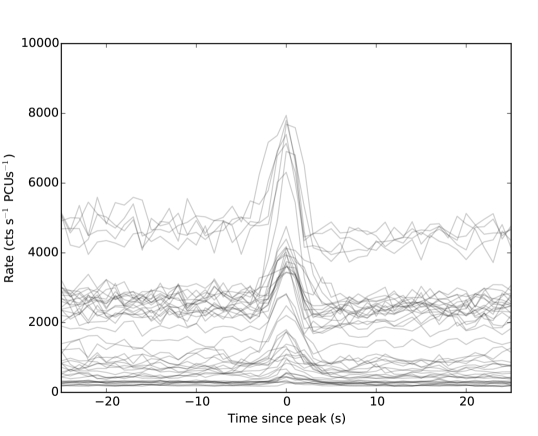
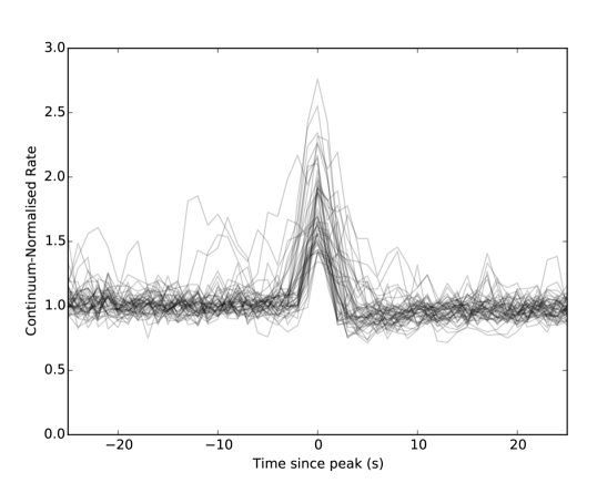
Figure 5.14: Top: a plot of every Miniburst, centred by the time of its peak, overlaid on top of each other. Bottom: a plot of every Miniburst in which count rates have been normalised by the persistent emission count rate during the observation from which each burst was observed.

Minibursts are all $\sim 5$ s in duration, and some show signs of a ‘dip’ feature similar to those seen in Normal Bursts. I find that the timescales of these dips are all $\lesssim 10$ s. I estimate ‘missing’ fluence in each dip by integrating the total persistent-rate-subtracted counts between the end of the burst and a point 10 s later. If this ‘missing fluence’ is less than half of the standard deviation in count rate multiplied by 5 s, which represents the smallest $<10$ s triangle-shaped dip which would be detectable above noise in a given dataset, I treat the dip in that outburst as not being detected.

Due to the relatively short duration and low amplitudes of Minibursts, I am unable to reliably discern whether they contain a single peak or multiple peaks. For this reason I do not fit them mathematically.

Parameters & Correlations

For each Miniburst, I extract the following parameters:

• Total burst fluence and burst fluence divided by persistent emission.

• Peak 1 s binned rate and peak rate divided by persistent emission.

• Rise time, fall time and total time.

The mean and standard deviation of each of these parameters, calculated from RXTE data, is presented in Table 5.5 for Outburst 1, Outburst 2 and the combined population of Minibursts from Outbursts 1 & 2. The standard deviations on the fluence and peak rates of Minibursts are very large, suggesting that these parameters are distributed broadly.

	Outburst 1		Outburst 2		Outbursts 1&2
	Mean	S.D.	Mean	S.D.	Mean	S.D.
Fluence	6792	5776	4474	3307	5422	4627
Peak Rate	3501	2851	2473	1664	2902	2293
Fluence/$k$	3.67	1.13	3.58	1.47	3.61	1.34
Peak Rate/$k$	1.90	0.37	1.76	0.28	1.82	0.32
Rise Time	2.33	0.8	2.03	1.1	2.15	1.0
Fall Time	2.32	0.9	2.35	1.0	2.32	0.9
Tot. Time	4.61	1.0	4.38	01.0	4.47	1.0

Table 5.5: A table showing the mean and standard deviation of 7 parameters of RXTE-sampled Minibursts from Outburst 1, Outburst 2 and both outbursts combined. Fluence is given in cts PCU^-1, peak rate is given in cts s^-1 PCU^-1 and rise, fall and total time are given in s. $k$ is the persistent emission rate during the observation in which a given burst was detected.

Using the Spearman’s Rank metric, I find only two correlations above the 5$\,\sigma$ level:

• Fluence is correlated with peak rate ($7.3\,\sigma$).

• Fluence divided by persistent rate is correlated with peak rate divided by persistent rate ($7.1\,\sigma$).

As in Normal Bursts, a correlation between peak rate and fluence is to be expected. However, due to the poor statstics associated with Miniburst parameters, it is likely that other parameter pairs are also correlated.

Colour Evolution

Minibursts show the greatest magnitude of evolution in colour of all the classes of burst. In Figure 5.15, I show how the hardness ratio between the 4–10 and 2–4 keV energy bands changes during an observation containing both a Miniburst and a Normal Burst. I find that the hardness ratio increases by $\sim 50\%$ in a Miniburst, significantly more than the change in hardness during Normal or Mesobursts. The statistics in minibursts were too poor to check for the presence of hysteresis.

Figure 5.15: A portion of observation 10401-01-16-00, featuring a Normal Burst ($\sim 30$ s) and a Miniburst ($\sim 410$ s). The top panel shows the total 2–10 keV lightcurve. The middle panel shows lightcurves from two different energy bands; the count rates from the soft energy band have been multiplied by 5.4 so they can more easily be compared with the hard energy band. The bottom panel shows the evolution over time of the ratio between the rates in the two bands. As can be seen in panels 2 and 3, the Miniburst has a significantly higher fractional amplitude in the 4–10 keV energy band than in the 2–4 keV band.

5.2.5 Mesobursts

I define Mesobursts as the set of all bursts with a persistent-emission-subtracted peak 1 s binned RXTE/PCA-equivalent count rate below 3000 cts s^-1 PCU^-1 in which the peak of the burst reaches at least $300\%$ of the persistent rate. Mesobursts account for 43 out of the 190 bursts identified for this study. They are observed in RXTE data from both Outbursts 1 & 2; in both cases they occur after the main outburst and before or during a rebrightening event. Mesobursts occurred between MJDs 50238 and 50248 in Outburst 1, and between 50562 and 50577 in Outburst 2; during these intervals, RXTE observed the source for a total of 44 ks. As no soft X-ray instrument monitored the Bursting Pulsar during the latter stages of Outburst 3, it is unclear whether Mesobursts occurred during this outburst. The one pointed observation of NuSTAR made during this time did not detect any Mesobursts.

Recurrence Time

Only 6 RXTE observations in Outburst 1, and 4 in Outburst 2, contain multiple Mesobursts. From my limited sample I find minimum and maximum recurrence times of $\sim 230$ and $\sim 1550$ s in Outburst 1 and minimum and maximum recurrence times of $\sim 310$ and $\sim 2280$ s in Outburst 2.

Structure

The structure of the main part of a Mesoburst is significantly more complex than in Normal Bursts, consisting of a large number of secondary peaks near the main peak of the burst. Mesobursts never show the post-burst ‘dip’ feature that we see in Normal Bursts or Minibursts, but they can show ‘plateaus’. In Figure 5.16 I show an example of a Mesoburst with a plateau similar to those seen after Normal Bursts, suggesting a connection between the two classes.

Figure 5.16: A lightcurve from RXTE/PCA observation 20078-01-17-00 from Outburst 2, showing an apparent ‘plateau’ feature after a Mesoburst.

In Figure 5.17 I show the lightcurves of all Mesobursts observed by RXTE overlayed on top of each other before (top panel) and after (bottom panel) being renormalised by persistent emission rate. It can be seen that the intensity and structure of these bursts is much more variable than in Normal Bursts (see Figure 5.8). However, each Mesoburst has a fast rise followed by a slow decay, and they occur over similar timescales of $\sim 10$–$30$ s.

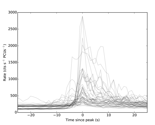
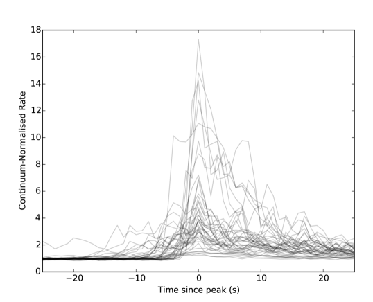
Figure 5.17: Top: a lightcurve of every Mesoburst, centred by the time of its peak, overlaid on top of each other. Bottom: a plot of every Mesoburst in which count rates have been normalised by the persistent emission count rate during the observation from which each burst was observed.

Parameters & Correlations

Due to the complexity structure of Mesobursts, I do not fit them mathematically as I did for Normal Bursts. Instead I extract the same parameters as for Minibursts (see the list in Section 5.2.4). The mean and standard deviation of each of these parameters, calculated from RXTE/PCA data, is presented in Table 5.6. Due to the relative low number of Mesobursts compared to Normal Bursts, I only present the results from the combined set of bursts in both Outbursts 1 & 2. In general, Mesobursts are longer in duration than Normal Bursts, and have significantly smaller amplitudes and fluences (compare e.g. Table 5.4).

	Mean	Standard Deviation
Fluence (cts PCU-1)	6067	6707
Peak Rate (cts s-1 PCU-1)	665.4	658.4
Fluence/$k$	48.6	32.8
Peak Rate/$k$	5.32	4.0
Rise Time (s)	6.95	4.9
Fall Time (s)	18.28	10.8
Total Time (s)	25.88	13.3

Table 5.6: A table showing the mean and standard deviation of 7 burst parameters of RXTE-sampled Mesobursts from Outbursts 1 & 2. $k$ is the persistent emission rate during the observation in which a given burst was detected.

Using the Spearman’s Rank metric, I find a number correlations above the 5$\,\sigma$ level:

• Fluence is correlated with peak rate ($>10\,\sigma$), peak rate divided by persistent rate ($6.7\,\sigma$), fall time ($6.8\,\sigma$) and total time ($6.0\,\sigma$).

• Fluence divided by persistent rate is correlated with peak rate divided by persistent rate ($7.3\,\sigma$).

• Peak rate is also correlated with peak rate divided by persistent rate ($7.4\,\sigma$), fall time ($5.8\,\sigma$) and persistent level ($6.2\,\sigma$).

• Rise time correlates with total time ($5.4\,\sigma$).

• Fall time correlates with total time ($>10\,\sigma$).

Again, the correlation between fluence and peak rate is expected, as is the correlation between peak rate and peak rate divided by persistent rate.

Colour Evolution

The hardness ratio of the emission from the source decreases significantly during Mesobursts, with the PCA 8–60/2–7 keV colour decreases from $\sim 0.6$ between bursts to $\sim 0.2$ at the peak of a burst. Due to the poor statistics of these features compared with Normal Bursts, I was unable to check for evidence of hardness-intensity hysteresis.

5.2.6 Structured ‘Bursts’

I define Structured Burst observations as observations in which the recurrence time between bursts is less than, or approximately the same as, the duration of a single burst. Structured Bursts constitute the most complex behaviour I find in my dataset. Unlike the other classes of burst A.A. and I identify, Structured Bursts are not easily described as discrete phenomena. I find Structured Bursts in 54 observations which are listed in Appendix B.

In both outbursts covered by RXTE, Structured Bursts occur in the time between the end of the main outburst and the start of a rebrightening event. In both cases these periods of Structured Bursts are preceded by a period populated by Mesobursts. Mesobursts occurred between MJDs 50248 and 50261 in Outburst 1, and between 50577 and 50618 in Outburst 2; during these intervals, RXTE observed the source for a total of 81 ks. Notably, as I show in Figure 5.18, one Outburst 1 RXTE lightcurve containing Structured Bursting also contains a bright Mesoburst.

Figure 5.18: A lightcurve from RXTE/PCA observation 10401-01-57-03, showing a Mesoburst occuring during a period of Structured Bursting.

In both outbursts, the amplitude of Structured Bursting behaviour decreases as the outburst approaches the peak of the rebrightening event. This amplitude continues to decrease as the Structured Burst behaviour evolves into the low-amplitude noisy variability associated with the source’s evolution towards the low/hard state.

Colour Evolution

I produce hardness-intensity diagrams for a number of Structured Bursting observations; I show a representative example in Figure 5.19. I find that hardness is strongly correlated with count rate during this class of bursting, but that the magnitude of the change in hardness is no greater than $\sim 30\%$. This is less than the change in hardness that I find during Normal or Minibursts. I also find no evidence of hysteretic hardness-intensity loops from Structured Bursts.

Figure 5.19: A 1 s-binned hardness-intensity diagram from RXTE observation 20078-01-23-00, showing that hardness tends to correlate with intensity during Structured Bursting. Data are binned to 8 s, and background has been estimated by subtracting mean count rates in the relevant energy bands from RXTE OBSID 30075-01-26-00.

Types of Structured Bursting

In Figure 5.20, I present a selection of lightcurves which show the different types of variability that can be seen during periods of Structured Bursting. These consist of a variety of patterns of flares and flat-bottomed dips, and both RXTE-observed outbursts show several of these different patterns of Structured Bursting. As all types of Structured Bursting have similar amplitudes and occur in the same part of each outburst, I consider them to be generated by the same physical process. I do not seperate these patterns into separate subclasses in this thesis.

Figure 5.20: A selection of RXTE lightcurves from Structured Bursting observations of the Bursting Pulsar. Top: a lightcurve from Outburst 1 showing flaring on timescales of $\sim 10$ s. Middle: a lightcurve from Outburst 1 showing the same flaring behaviour with an additional slower modulation over $\sim 50$ s. Bottom: a lightcurve from Outburst 2 showing a regular sequence of flat-bottomed dips and multi-peaked flaring. These show the wide variety of variability patterns that I classify as ‘Structured Bursting’.

5.3 Discussion

I analyse all available X-ray data from the first 3 outbursts of the Bursting Pulsar. The bursting behaviour evolves in a similar way during these outbursts, strongly associating them with the Bursting Pulsar and suggesting an underlying connection between the classes of burst. I also find that both Outbursts 1 & 2 showed ‘rebrightening events’ similar to those seen in a number of other LMXBs (e.g. Wijnands et al.,, 2001; Patruno et al.,, 2016), including IGR J17091.

I find that the X-ray bursts from these data can be best described as belonging to four phenomenological classes: Normal Bursts, Minibursts, Mesobursts and Structured Bursts. For each of these four classes, I collect a number of statistics to shed light on the physical mechanisms that generate these lightcurve features.

Normal Bursts and Minibursts both represent the ‘Type II’ bursting behaviour which is observed most commonly from this source. Mesobursts occur much later on in the outburst and show fast-rise slow-decay profiles; they are generally much fainter and more structured than Normal Bursts. Finally, Structured Bursts form continuous highly structured regions of variability over timescales of days. All Normal Bursts and some Minibursts show count rate ‘dips’ after the main burst, while Mesobursts and Structured Bursts do not. In addition to this, some Normal and Mesobursts show count rate ‘plateaus’; regions of roughly stable count rate above the persistent level which last for $\sim 10$s of seconds. These features are also sometimes seen in Mesobursts, while Minibursts and Structured Bursts never show these structures.

Here I discuss these results in the context of models proposed to explain Type II bursting. I also compare my results with those of previous studies on bursting in both the Bursting Pulsar and the Rapid Burster.

5.3.1 Evolution of Outburst and Bursting Behaviour

In general, Outburst 1 was brighter than Outburst 2, with the former having a peak 2–60 keV intensity a factor of $\sim 1.7$ greater than the latter. However, in Figure 5.1 I show that both outbursts evolve in a similar way. In both outbursts, the intensity of the Bursting Pulsar reaches a peak of order $\sim 1$ Crab before decreasing over the next $\sim 100$ days to a level of a few tens of mCrab. A few 10s of days after reaching this level, the lightcurves of both outbursts show a pronounced ‘rebrightening’ event, during which the intensity increases to $\sim 100$ mCrab for $\sim 10$ days. Outburst 1 shows a second rebrightening event $\sim 50$ days after the first. It is unclear whether any rebrightening events occurred in Outburst 3 due to a lack of late-time observations with soft X-ray telescopes. X-ray ‘rebrightening’ events have been seen after the outbursts of a number of other LMXBs with both neutron star and black hole primaries: including SAX J1808.4-3658 (Wijnands et al.,, 2001), XTE J1650-500 (Tomsick et al.,, 2003) and IGR J17091-3624 (see Section 4.2.1).

As I have shown in Figures 5.5 & 5.6, the nature of bursts from the Bursting Pulsar evolves in a similar way in both Outbursts 1 & 2. Starting from around the peak of each outburst, both Normal and Minibursts are observed. The fluence of these bursts decrease over time as the X-ray intensity of the source decreases, before bursting shuts off entirely when the 2–16 keV flux falls below $\sim 0.1$ Crab. After a few 10s of days with no bursts, bursting switches back on in the form of Mesobursts; this occurs during the tail of a rebrightening event in Outburst 1, but in the tail of the main outburst in Outburst 2. Mesobursting continues until the 2–16 keV source flux falls below $\sim 0.03$ Crab, at which point I observe the onset of Structured Bursting. In both Outbursts, Structured Bursting stops being visible a few 10s of days later during the start of a rebrightening event. Because this evolution is common to both of the outbursts observed by RXTE, this strongly indicates that the nature of bursting in the Bursting Pulsar is connected with the evolution of its outbursts. Additionally, with the exceptions of Normal and Minibursts, I show that each class of burst is mostly found in a distinct part of the outburst corresponding to a different level of persistent emission.

In Figure 5.21, I show lightcurves from Outburst 2 taken a few days before and after the transition from Mesobursts to Structured Bursting. We can see that, as the system approaches this transition, Mesobursts become more frequent and decrease in amplitude. Additionally in Figure 5.18 I show a lightcurve which contains both a Mesoburst and Structured Bursting. I find that, instead of a well-defined transition between these bursting classes, there is a more gradual change as Mesobursting evolves into Structured Bursting.

The transition between Normal Bursts and Mesobursts, however, is not smooth; in both outbursts these two classes of bursting are separated by $\sim 10$ day gaps in which no bursts of any kind were observed at all. If all my classes of burst are caused by the same or similar processes, any model to explain them will also have to explain these periods with no bursts.

Figure 5.21: A series of lightcurves from RXTE/PCA observations of Outburst 2, showing a gradual evolution from Mesobursts to Structured Bursting over a period of $\sim 30$ days. Each inset lightcurve is plotted with the same $y$-scaling, and each corresponds to 2 ks of data.

5.3.2 Parameter Correlations

I extracted a number of phenomenological parameters from each Normal Burst, Miniburst and Mesoburst. For Normal Bursts, I extracted a large number of parameters by fitting a phenomenological model described in Section 5.2.3. For Minibursts and Mesobursts I extracted recurrence times and persistent emission-subtracted peak rates; I also calculated burst fluences by integrating the persistent emission-subtracted rate over the duration of the burst. I do not extract similar parameters for Structured Bursts due to their complex nature.

In all three of the classes of burst I consider, I found that fluence and peak rate correlate strongly with persistent emission. For each type of burst, the slope of these correlations is consistent with being equal during Outbursts 1 & 2.

I also compared the Normal Bursts in Outburst 1 with the Normal Bursts in Outburst 2. The only significant statistical differences I found between these two populations were in the burst peak rate and the burst fluence; both of these parameters are generally higher for Normal Bursts in Outburst 1. As both of these parameters strongly depend on the persistent emission, both of these differences can be attributed to the fact that Outburst 1 was significantly brighter at peak than Outburst 2.

For Normal Bursts, I found additional correlations. Of particular note, I found that both the fall time and the recovery timescale of a ‘dip’ is proportional to its amplitude, which has implications for the possible mechanism behind these features. I discuss this further in Section 5.3.5.

My findings strongly suggest that the properties of Normal, Mini and Mesobursts all depend on the persistent luminosity of the Bursting Pulsar. Assuming that this persistent luminosity is proportional to $\dot{M}$, this suggests that all classes of bursting are sensitive to the accretion rate of the system. Additionally, with the exceptions of Normal and Minibursts, I find that each class of burst is mostly found in a distinct part of the outburst corresponding to a different level of persistent emission. I suggest that Normal, Meso and Structured Bursts may in fact be manifestations of the same physical disk instability but at different accretion rates. This is supported by the observation of a Mesoburst during a period of Structured Bursting, which I show in the lightcurve in Figure 5.18. This shows that the conditions for both Mesobursts and Structured Bursting can be met at the same time.

5.3.3 Comparison with Previous Studies

In their study of bursts in the Bursting Pulsar, Giles et al., (1996) found evidence for three distinct classes of Type II bursts in the Bursting Pulsar:

• ‘Bursts’ (hereafter G₁ Bursts to avoid confusion), the common Type II bursts seen from the source.

• ‘Minibursts’ (hereafter G₂ Bursts), with smaller amplitudes up to $\sim 2$ times the persistent emission level.

• ‘Microbursts’ (hereafter G₃ Bursts), second-scale bursts with amplitudes of $\sim 50$–$100\%$ of the persistent level.

We find that Giles et al.,’s G₁ category contains the bursts that I identify as Normal Bursts, while my Miniburst category contains the same bursts as Giles et al.,’s G₂ category. Giles et al., only consider bursts up to MJD 50204 in their classification, and they could not classify any bursts that I identify as Mesobursts; under their framework, I find that Mesobursts would also be categorised as G₁. I present the full mapping between Giles et al.,’s classes and my classes in a schematic way in Table 5.7.

My Class	Giles et al., Class
Normal Bursts	G1
Mesobursts	G1
Minibursts	G2
Structured Bursts	-
-	G3

Table 5.7: A table showing how my burst classes map to those described in Giles et al., (1996). Giles et al., do not consider the times during the outburst when Structured Bursts appear, and I consider G₃ bursts described by Giles et al., to be consistent with flicker noise.

Giles et al., (1996) note the presence of both dips and plateaus in Normal Bursts. To calculate the fluence of each main burst and its associated dip, Giles et al., integrate the total persistent-emission-subtracted counts in each feature. They calculate that ratio between burst fluence and ‘missing’ dip fluence ($\phi_{B}/\phi_{d}$) is between 0.26 and 0.56 in Outburst 1 before correcting for dead-time effects. Using bursts in which my mathematical fit gave well-constrained ($>5\,\sigma$) values for both burst and dip fluence, I find that $\phi_{B}/\phi_{d}$ is between 1.3 and 2.0 in Outburst 1 and between 1.3 and 2.9 in Outburst 2. My values differ significantly from those reported from Giles et al.,; this is likely due to differing definitions of the persistent emission level and the start and end times of each dip, as Giles et al., do not report how they define these features.

My values for the ratios between burst and dip fluences, as well as those of Giles et al.,, are affected by dead-time. These effects cause the fluence of bursts to be under-reported, as can be inferred from Figure 5.23, but the integrated counts in dips are not significantly affected (Giles et al.,, 1996). Therefore correcting for dead-time can only increase the value of $\phi_{B}/\phi_{d}$, and my result shows that the fluence of a burst is always greater than the fluence ‘missing’ from a dip.

T.O. and I find evidence of significant colour evolution during both Normal Bursts and Minibursts, which is strongly indicative of a spectral evolution (see also e.g. Woods et al.,, 1999). Further work on the time-resolved spectra of this source will likely allow us to better understand the underlying physics of its behaviour.

Using data from the KONUS experiments aboard the GGS-Wind and Kosmos-2326 satellites, Aptekar et al., (1998) have previously found that the recurrence times between consecutive bursts in Outburst 1 are distributed with a constant mean of $\sim 1776$ s. This is substantially longer than the value of 1209 s that I find for Outburst 1, but my value is likely an underestimate due to a selection bias caused by the relatively short pointings of RXTE.

Using Chandra and XMM-Newton data, I find a mean recurrence time for Outburst 3 of 1986 s; as pointings with these instruments are significantly longer than the burst recurrence timescale, windowing effects are negligible. As this value is close to the value that Aptekar et al., (1998) find for mean recurrence time, my result is consistent with the burst rate in all three outbursts being approximately the same.

Previous studies with CGRO/BATSE have found that the burst rate during the first few days of Outbursts 1 & 2 was significantly higher than during the rest of each outburst (Kouveliotou et al., 1996b, ; Woods et al.,, 1999). As RXTE did not observe either of these times, I am unable to test this result with my dataset.

5.3.4 Comparison with other objects

Another natural comparison to the Bursting Pulsar is the Rapid Burster (Lewin et al., 1976a, ), a neutron star LMXB in the globular cluster Liller I. This object is the only LMXB other than the Bursting Pulsar known to unambiguously exhibit Type II bursting behaviour during outbursts. Rappaport and Joss, (1997) have previously proposed that the Bursting Pulsar, the Rapid Burster and other neutron star LMXBs form a continuum of objects with different magnetic field strengths.

I compare my study of bursts in the Bursting Pulsar with studies of Type II bursts in the Rapid Burster, particularly the detailed population study performed by Bagnoli et al., (2015). Bagnoli et al., (2015) found that Type II bursting begins during the decay of an outburst in the Rapid Burster. This is the same as what we see in the Bursting Pulsar, where I find Normal Bursting behaviour starts during the outburst decay. Bagnoli et al., (2015) found that all bursting in the Rapid Burster shuts off above an Eddington Fraction of $\gtrsim 0.05$, whereas I find that bursting in the Bursting Pulsar shuts off below a 2–16 keV flux of Eddington fraction of $\sim 0.1$ Crab: assuming that the peak persistent luminosity of the Bursting Pulsar was approximately Eddington Limited (e.g. Sazonov et al.,, 1997), this value corresponds to an Eddington fraction of order $\sim 0.1$. This suggests that Type II bursting in these two objects happen in very different accretion rate regimes.

Bagnoli et al., (2015) showed that bursting behaviour in the Rapid Burster falls into a number of ‘bursting modes’, defined by the morphology of individual Type II bursts. In particular, they find that Type II bursts in the Rapid Burster fall into two classes (see also Marshall et al.,, 1979), lightcurves of which I reproduce in Figure 5.22:

Figure 5.22: RXTE lightcurves of representative Long (top) and Short (bottom) Type II bursts from the Rapid Burster. These bursts were identified and classified by Bagnoli et al., (2015).

• Short near-symmetric Bursts with timescales of $\sim 10$s of seconds and peak rates near the Eddington Limit.

• Long bursts with a fast rise, a long $\sim 100$ s plateau at peak rate followed by a fast decay. The level of the plateau is generally at or near the Eddington Limit.

Short bursts are very similar in shape to Normal Bursts in the Bursting Pulsar, but I find no analogue of long bursts in my study. Bagnoli et al., (2015) suggests that the ‘flat-top’ profile of long bursts could be due to the effects of near-Eddington accretion, and they show that the intensity at the top of these bursts is close to Eddington limit. Previous works have shown that the persistent emission of the Bursting Pulsar is Eddington-limited at peak, and therefore bursts from the Bursting Pulsar are significantly super-Eddington (Sazonov et al.,, 1997). I suggest, therefore, that Long Bursts cannot occur in systems with a persistent rate approaching the Eddington Limit. This could explain why Long Bursts are not seen during periods of Normal Bursting in the Bursting Pulsar (during which the persistent emission is $\gtrsim{20}$% of Eddington), but it remains unclear why these features are not seen later in each outburst when the Bursting Pulsar is fainter. Alternatively, all the differences we see between bursts produced by the Rapid Burster and the Bursting Pulsar could be explained if the physical mechanisms behind these bursts are indeed different between the objects.

Bagnoli et al., (2015) also find a number of correlations between burst parameters in the Rapid Burster, which I can compare with my results for the Bursting Pulsar. I find a number of similarities between the two objects:

• The fluence of a burst correlates with its amplitude.

• The duration of a burst does not correlate with the persistent emission.

• The recurrence time between consecutive bursts does not depend on the persistent emission.

There are also a number of differences between the set of correlations between burst parameters in these two systems:

• Burst duration is correlated with burst fluence in the Rapid Burster, but these have not been seen to correlate in the Bursting Pulsar.

• Burst duration, peak rate and burst fluence are all correlated with burst recurrence time in the Rapid Burster. I have not found any of these parameters to correlate with burst recurrence time in the Bursting Pulsar.

• Peak rate and burst fluence correlate with persistent emission in the Bursting Pulsar, but this is not true for bursts of a given type in the Rapid Burster.

As the neither the fluence nor the class of a burst in the Rapid Burster depend strongly on persistent emission, and hence $\dot{M}$, this suggests that the process that triggers Type-II bursts in this source is not strongly dependent on the global accretion rate. However the strong correlations between persistent emission and burst peak and fluence I find in the Bursting Pulsar show that the energetics of individual bursts strongly depend global accretion rate at that time.

It has previously been noted that consecutive Normal Bursts in the Bursting Pulsar do not show a strong correlation between recurrence time and fluence (Taam and Lin,, 1984; Lewin et al.,, 1996, however see Aptekar et al.,, 1997). This correlation would be expected if the instability took the form of a relaxation oscillator, as it does in the Rapid Burster (Lewin et al., 1976b, ). However, I also find that the arrival times of Normal Bursts from the Bursting Pulsar are not consistent with a Poisson distribution with constant mean. This implies either that bursts are also not independent events in the Bursting Pulsar, or that the frequency of these bursts is not constant throughout an outburst as reported by Aptekar et al., (1998).

In Chapter 6 I discuss the possibility that some of the behaviour in the Bursting Pulsar could be due to fluctuations in the magnetospheric radius of the system close to the co-rotation radius. This behaviour, referred to in this thesis as ‘hiccup’ accretion, (e.g. Bogdanov et al.,, 2015; Ferrigno et al.,, 2014) is also seen in ‘Transitional Millisecond Pulsars’ (TMSPs): objects which alternate between appearing as X-ray pulsars and radio pulsars (see e.g. Archibald et al.,, 2009; Papitto et al., 2013a, ).

5.3.5 Comparison with Models of Type II Bursts

All of the models of Type II bursting which we discuss in Section 2.4.1 are able to reproduce some of the features we see from bursts in the Bursting Pulsar. In particular, the ‘dip’ we see after Normal Bursts has previously been interpreted as being caused by the inner disk refilling after a sudden accretion event (e.g. Younes et al.,, 2015). As these dips are also seen after some Minibursts, we could also interpret Minibursts as being caused by a similar cycle. To test this idea, in Figure 5.23 I present a scatter plot of the burst and dip fluences for all Normal Bursts and Minibursts. In both classes of burst, there is a strong correlation between these two parameters. I find that a power law fit to the Normal Bursts in this parameter space also describes the Minibursts. This suggests that the same relationship between burst fluence and missing dip fluence holds for both types of burst, although the two populations are not continuous. This suggests that Minibursts are energetically consistent with being significantly fainter versions of Normal Bursts.

Figure 5.23: A scatter plot showing the relationship between burst fluence and ‘missing’ dip fluence for Normal Bursts (black) and Minibursts (Red), with the best fit power law plotted in solid blue. A power law fit to just the Normal Bursts (blue dashed line) also approaches the Minibursts. Note that the Normal Bursts plotted in grey were not used to calculate this latter fit, as the effects of instrumental dead-time cause high burst fluences to be under-reported. Upper limits on Miniburst dip fluences are shown with arrows.

The models of Spruit and Taam, (1993) and Walker, (1992) have shortcomings when used to describe the Bursting Pulsar. Walker, (1992) state that their model only produces Type II bursts for a very specific set of criteria on the system parameters. One of these criteria is an essentially non-magnetic ($B=0$) neutron star. This is inconsistent with observations of cyclotron lines from the Bursting Pulsar and the presence of a persistent pulsar, both of which suggest a surface field strength of order 10¹¹ G (Doroshenko et al.,, 2015).

Unlike models based on viscous instability, the model of Spruit and Taam, (1993) does not impose a correlation between burst fluence and burst recurrence time (see e.g. the evaluation of this model in the context of the Rapid Burster performed by Bagnoli et al.,, 2015). However, it does predict a strong correlation between burst recurrence time and mean accretion rate, which is not consistent with my results for the Bursting Pulsar.

In general, I find that models established to explain bursting in the Rapid Burster are poor at explaining bursting in the Bursting Pulsar. Any model which can produce Type II bursting in both systems fails to explain why other systems do not also show this behaviour. My results suggest that Type II bursts in the Rapid Burster and the Bursting Pulsar may require two separate models to be explained.

Evidence of Thermonuclear Burning

I also consider the possibility that some of my observations could be explained by thermonuclear burning on the Bursting Pulsar. A thermonuclear origin for the main part of Normal Bursts has been ruled out by previous authors (e.g. Lewin et al.,, 1996), but it is less clear that associated features could not be explained by this process.

It has been shown that, above a certain accretion rate, thermonuclear burning on the surface of a neutron star should be stable; below this rate, thermonuclear burning takes place in the form of Type I bursts (e.g. Fujimoto et al.,, 1981; Bildsten,, 1995). Bildsten and Brown, (1997) have previously studied which form thermonuclear burning on the Bursting Pulsar would take. They find that the presence and profile of a thermonuclear burning event on the Bursting Pulsar would be strongly dependent on both the accretion rate $\dot{M}$ and the magnetic field strength $B$. They predict that, for $B\gtrsim 3\times 10^{10}$ G, burning events would take the form of a slowly propagating burning front which would result in a low-amplitude X-ray burst with a timescale of several minutes. Measurements of the Bursting Pulsar taken during Outburst 3 suggest a surface field strength of $>10^{11}$ G, in turn suggesting that the Bursting Pulsar exists in the regime in which this burning behaviour is possible.

The ‘plateau’ events after Normal Bursts are consistent with the slow burning predicted by Bildsten and Brown, (1997). This picture is consistent with models for Type II X-ray bursts involving spasmodic accretion events (e.g. Spruit and Taam,, 1993; Walker,, 1992), as plateaus always occur after a Type II-like burst has deposited a large amount of ignitable material onto the neutron star surface. However in this picture it would be unclear why many Normal Bursts do not show this plateau feature. Mesobursts can also exhibit plateaus, and are therefore may also be products of spasmodic accretion onto the neutron star.

However, the interpretation of Mesobursts as being caused by discrete accretion events is difficult to reconcile with the fact that these features never show dips. Bildsten and Brown, (1997) show that, at smaller values of $\dot{M}$, nuclear burning on the Bursting Pulsar could become unstable. Mesobursts are only seen during the latter stages of Outbursts 1 & 2, when the accretion rate is well below 0.1 Eddington. An interesting alternative possibility is that Mesobursts are a hybrid event, consisting of a flash of unstable thermonuclear X-ray burning followed by a slower quasi-stable burning of residual material in the form of a propagating burning front.

This picture would also be able to explain why Mesobursts are only seen during the latter parts of each outburst. As the accretion rate onto the Bursting Pulsar approaches Eddington during the peak of its outbursts, it is likely that the accretion rate is high enough that only stable burning is permitted. During the smaller rebrightening events after the main part of each outburst, the accretion rate is $\sim 1$–2 orders of magnitude lower, and hence the system may then be back in the regime in which Type I burning is possible. Additional studies of the spectral evolution of Mesobursts will be required to further explore this possibility.

Previous authors have discussed the possibility of a marginally stable burning regime on the surface of neutron stars (not to be confused with the previously mentioned quasi-stable burning). In this regime, which occurs close to the boundary between stable and unstable burning, Heger et al., (2007) showed that an oscillatory mode of burning may occur. They associated this mode of burning with the mHz QPOs which have been observed in a number of neutron star LMXBs (e.g. Revnivtsev et al.,, 2001; Altamirano et al., 2008c, ). These QPOs only occur over a narrow range of source luminosities, show a strong decrease in amplitude at higher energies, and they disappear after a Type I burst (e.g. Altamirano et al., 2008c, ).

Lightcurves of objects undergoing marginally stable burning qualitatively resemble those of Structured Bursting in the Bursting Pulsar, raising the possibility of a thermonuclear explanation for Structured Bursting. However, as I show in Figure 5.5, Structured Bursting during Outburst 1 occurred during a period of time in which the Bursting Pulsar’s luminosity changed by $\sim 1$ order of magnitude. In addition to this, in Figure 5.18 I show an example of a Mesoburst during a period of Structured Bursting. If Mesobursts can be associated with Type I bursts, any marginally stable burning on the surface of the Bursting Pulsar should have stopped after this event. Due to these inconsistencies with observations of marginally stable burning on other sources, it is unlikely that Structured Bursting is a manifestation of marginally stable burning on the Bursting Pulsar.

Linares et al., (2012) observed yet another mode of thermonuclear burning during the 2010 outburst of the LMXB Terzan 5 X-2. They observed a smooth evolution from discrete Type I bursts into a period of quasi-periodic oscillations resembling Structured Bursting. This behaviour resembles the evolution I observe between Mesobursts and Structured Bursting in Outbursts 1 & 2 of the Bursting Pulsar (as shown in Figure 5.21; compare with Figure 1 in Linares et al.,, 2012). However there are a number of differences between the evolutions seen in both objects. In Terzan 5 X-2 the recurrence timescale of Type I bursts during the evolution is strongly related to the accretion rate of the source at the time, whereas there is no such strong relation between the two in Mesobursts from the Bursting Pulsar. Additionally, the quasi-periodic oscillations in Terzan 5 X-2 evolved smoothly back into Type I bursts later in the outburst, whereas Structured Bursting does not evolve back into Mesobursts in the Bursting Pulsar. As such, it is unclear that Mesobursts and Structured Bursting can be associated with the unusual burning mode seen on Terzan 5 X-2.

5.4 Conclusions

I analyse all X-ray bursts from the Bursting Pulsar seen by RXTE/PCA during its first and second outbursts, as well as bursts seen by other missions during the third outburst of the source. I conclude that these bursts are best described as belonging to four separate classes of burst: Normal Bursts, Mesobursts, Minibursts and Structured Bursts. I find that the bursting behaviour in these four classes evolves in a similar way throughout the first two outbursts of the Bursting Pulsar. I present a new semi-mathematical model to fit to the Normal Bursts in this object. Using this new framework, I will be able better quantify Bursting-Pulsar-like X-ray bursts when they are observed in other objects in the future.

I find the bursts in the Rapid Burster and the Bursting Pulsar to be different in burst profile, peak Eddington ratio, and durations. While the fluence of bursts in the Bursting Pulsar depend strongly on the persistent emission at the time, this is not the case in the Rapid Burster. Additionally the waiting time between bursts in the Rapid Burster depends heavily on the fluence of the preceding burst, but I do not find this in the Bursting Pulsar. Therefore, it would be reasonable to conclude that the bursting in these two objects is generated by two different mechanisms.

However, it is also important to note a number of similarities between the Bursting Pulsar and the Rapid Burster. Bursting behaviour in both objects depends on the global accretion rate of the system and the evolution of its outbursts. Additionally, the recurrence times of bursts do not depend on persistent emission in either object, and nor does the duration of an individual burst. Notably while Type II bursts in the Rapid Burster only occur at luminosities $L\lesssim 0.05L_{Edd}$, I find that Normal bursts in the Bursting Pulsar only occur at $L\gtrsim 0.1L_{Edd}$. There is no overlap between the luminosity regimes, in terms of the Eddington Luminosity, at which bursting is observed in the two objects. This leads to the alternative hypothesis that bursts in the two systems may be caused by similar processes, but that these processes take place in very different physical regimes.

Chapter 6 The Bursting Pulsar GRO J1744-28: the Slowest Transitional Pulsar?

I’ll keep the sun behind us. You’ve spent your entire life in the dark, I doubt that seeing something that bright would do you any good.

Lance Abell - Take the Sky

In Chapter 5, I performed a detailed analysis of all archival X-ray data of bursting behaviour in the Bursting Pulsar (including RXTE, Swift, Chandra, XMM-Newton, Suzaku, NuStar, and INTEGRAL). I found that the bursting phenomenology in the Bursting Pulsar is much richer than previously thought (e.g. Giles et al.,, 1996): the characteristics of the bursts evolve with time and source luminosity. Near the end of this evolution, I observed periods of highly-structured and complex high-amplitude X-ray variability. I refer to this variability as ‘Structured Bursting’, and it is unlike what is seen in most other LMXBs.

In Section 5.3.5, I discuss the possibility that Structured Bursting is a manifestation of quasi-stable nuclear burning on the surface of the neutron star. However as other types of burst can occur during periods of Structured Bursting without disrupting this behaviour (see e.g. Figure 5.18), I consider this scenario to be unlikely. As such, we must consider alternative explanations. In this chapter I present the hypothesis that Structured Bursting is related to so-called ‘hiccup accretion’, a phenomenon seen in Transitional MilliSecond Pulsars (TMSPs).

The results I present in this chapter have been published as Court et al., 2018b .

6.1 Transitional Millisecond Pulsars

Millisecond Pulsars are old radio pulsars with spin periods of order $\sim 10$ ms (Backer et al.,, 1982). They have long been believed to be the end product of systems containing a neutron star in an LMXB. In these systems, matter from a Roche-lobe overflowing star donates angular momentum to a Neutron star, spinning it up to frequencies of several 100 Hz (Alpar et al.,, 1982). A number of fast-spinning X-ray pulsars (accreting Millisecond Pulsars, or AMXPs) have been found in LMXBs (e.g. Wijnands and van der Klis,, 1998; Altamirano et al., 2008a, ; Patruno et al.,, 2017; Sanna et al., 2017a, ), seemingly confirming this physical picture. At the end of this so-called ‘recycling’ process, the system should transition from an accretion-powered pulsar to a rotation-powered pulsar. As such, it has long been expected that such a transition could be observed by finding a system which changes its character from an accreting Neutron star at one time to a radio pulsar at some later time. Subsequently a small family of 7 candidate objects have been discovered or proposed: these are referred to as Transitional Millisecond Pulsars (TMSPs).

The first of these objects, PSR J1023+0038, was identified by Archibald et al.,, 2009. Although it appeared as a non-accreting radio pulsar at the time of identification in 2009, previous optical studies showed that this system contained an accretion disk in 2002 (Szkody et al.,, 2003). As such, the pulsar in this system must have switched from an accreting phase to a radio pulsar phase at some point between 2003 and 2009, confirming the identification of this system as a TMSP. The pulsar in this system has a spin period of 1.69 ms, and the companion is a star with a mass between $\sim$0.14–0.42 M_⊙. Archibald et al.,, 2009 suggested that the low X-ray luminosity of PSR J1023+0038 in its accreting phase was due to accretion taking place in the propeller regime (see Section 2.2.2). As previously discussed, whether a system is in the propeller regime depends on its spin and its magnetic field strength (see also Lewin et al.,, 1988). Additionally, below a certain accretion rate, no stable balance between ram pressure and radiation pressure can form and any disk is ejected from the system (e.g. Campana et al.,, 1998). Archibald et al.,, 2009 suggested that the current accretion rate in PSR J1023+0038 is only slightly below this critical value, and that any small increase in accretion rate could cause accretion in this system to resume. They suggested the possibility of TMSP systems which flip back and forth between accreting and radio pulsar phases multiple times.

Papitto et al., 2013a, identified IGR J18245-2452 as the first known pulsar to switch from a radio pulsar to an AMXP and back to a radio pulsar. This source was first observed as a radio pulsar (Manchester et al.,, 2005), before being observed several years later by XMM-Newton (Eckert et al.,, 2013) as an AMXP. Several months after the XMM-Newton observation, Papitto et al., 2013b, found that the source had reactivated as a radio pulsar during X-ray quiescence. The pulsar in this system has a period of 3.93 ms, and the companion star has a mass of $>0.17$ M_⊙ (Papitto et al., 2013a, ). During the 2013 outburst of IGR J18245-2452, Ferrigno et al.,, 2014 reported the presence of high-amplitude variability in the X-ray lightcurve. They interpreted this as being due to the accretion rate $\dot{M}$ being very close to the critical rate at which the propeller effect begins to dominate the flow geometry. In this regime, small fluctuations in $\dot{M}$ cause so-called ‘hiccups’, in which matter alternates between being ejected by the propeller effect and being accreted onto the neutron star poles (see our discussion of this effect in Section 2.2.3). Similar X-ray variability has subsequently been found in lightcurves from outbursts during the accreting phase of PSR J1023+0038 (Bogdanov et al.,, 2015), suggesting that this variability is somehow intrinsic to TMSPs as a class of objects.

1FGL J1227.9-4852 was first identified in the first Fermi/LAT source catalogue (Abdo et al.,, 2010). Hill et al.,, 2011 found that the $\gamma$-ray spectral characteristics of this source are consistent with known millisecond radio pulsars, although no radio pulsations were found. They suggested that this object could be associated with the X-ray source XSS J12270-4859. Before 2009, XSS J12270-4859 showed optical emission lines typical of an accretion disk (Pretorius,, 2009). Hill et al.,, 2011 suggested that XSS J12270-4859 may also be a TMSP, which switched from an accreting phase to a radio pulsar millisecond pulsar phase between 2009 and 2011. Subsequent studies have found pulsations in both the radio (Roy et al.,, 2015) and $\gamma$-ray (Johnson et al.,, 2015) emissions of this source, confirming the system contains a pulsar and establishing its spin period at 1.69 ms.

XMM J174457-2850.3 is a neutron star X-ray binary. Although no X-ray or radio pulsations have been detected due to the faintness of the source, Degenaar et al., 2014b, have found that the X-ray variability properties of this source are similar to those seen in other TMSPs. This object also exhibits extended low-luminosity states during outbursts, which Degenaar et al., 2014b, suggest may be symptomatic of TMSPs.

3FGL J1544.6-1125 was also first identified in Fermi/LAT data. Bogdanov and Halpern,, 2015 associated this object with the X-Ray source 1RXS J154439.4-112820. Due to the presence of $\gamma$-rays, as well as the presence of variability in the X-ray lightcurve similar to IGR J18245-2452, they proposed that this object is a TMSP in the accreting state. However, no pulsations from this system have been detected in the X-ray or the radio, so the pulsar period is not known. Bogdanov and Halpern,, 2015 found a bimodality in count rate during the period of X-ray variability, suggesting that this behaviour can be explained as quick transitions between three quasi-stable accretion modes which they refer to as ‘low’ , ‘high’ and ‘flaring’. This effect has also been seen in the TMSP IGR J18245-2452 (Ferrigno et al.,, 2014).

Strader et al.,, 2016 identified the $\gamma$-ray source, 3FGL J0427.9-6704, as a TMSP. They found that this source also displays X-ray variability similar to what is seen from the other known TMSPs. Finally, Rea et al.,, 2017 have proposed that the X-ray source XMM J083850.4-282759 may also be a TMSP. Although this source has not been detected in the gamma or the radio, the authors argued that X-ray variability coupled with X-ray flaring seen from this object is reminiscent of similar behaviour seen in other TMSPs during subluminous disk states.

The phenomenology of currently known TMSPs is varied, and different methods have been used to conclude (or propose) that each individual system belongs to this class. The fact that 6 of the 7 objects show similar patterns of X-ray variability during outburst suggests that this variability can be used as an indication that a system may be a TMSP.

6.2 Comparison: TMSPs vs. the Bursting Pulsar

Rappaport and Joss,, 1997 have previously suggested that the Bursting Pulsar represents a slow X-ray pulsar nearing the end of its accreting phase. As such it is natural to compare this system with TMSPs, which are also believed to be systems approaching this evolutionary stage. In addition to this, Degenaar et al., 2014b, have previously noted that the Bursting Pulsar shows extended low-luminosity states during outburst, similar to those seen in the TMSP candidate XMM J174457-2850.3.

Figure 6.1: Top: 2–15 keV XMM lightcurve from the TMSP PSR J1023+0038. Middle: 2–60 keV RXTE lightcurves from the Bursting Pulsar during its 1996 and 1997 outbursts, showing similar variability patterns to those seen in PSR J1023+0038. Bottom: 2–15 keV XMM lightcurve from the TMSP IGR J18245-2452. XMM lightcurves are shown from 2–15 keV so that they can be more directly compared with RXTE.

In Figure 6.1, I show RXTE lightcurves of ‘Structured Bursting’ from the Bursting Pulsar alongside lightcurves from periods of ‘hiccup’ variability observed in the confirmed TMSPs PSR J1023+0038 and IGR J18245-2452. All three sources show similar patterns of X-ray variability:

• Plateaus: periods of approximately constant count rate with high-amplitude flicker noise (all plateaus in a given observation have approximately the same mean rate),

• Dips: Periods of low count rate ($\lesssim 0.5$ of the rate in plateaus) with significantly less flicker noise, and

• Flares: Relatively short-lived increases of the count rate to values $\gtrsim 2$ times greater than the rate during plateaus.

In TMSPs, these features are interpreted as representing three quasi-stable accretion modes: the ‘high’, ‘low’ and ‘flaring’ modes respectively (e.g. Bogdanov et al.,, 2015). The most significant difference is that, in general, the variability in the Bursting Pulsar occurs on timescales $\sim 1$ order of magnitude longer than those in TMSPs.

In Figure 6.2 I show histograms of the 1 s-binned count-rate from all RXTE observations of Structured Bursting in the 1996 (left) and 1997 (right) outbursts of the Bursting Pulsar. As is the case for TMSPs, the histograms can be described with a number of log-Normally distributed populations: 3 populations in the 1996 outburst and 2 in the 1997 outburst. It is unclear why a population would be absent from the 1997 outburst, but some TMSPs have been observed to miss the ‘high’ mode during hiccup accretion (e.g. IGR J18245-2452, Ferrigno et al.,, 2014).

Figure 6.2: Histograms of the 1 s binned count rates from all RXTE observations of Structured Bursting in the 1996 (left) and 1997 (right) outbursts of the Bursting Pulsar. For the 1996 outburst, I fit the distribution with three Gaussians, while for the 1997 outburst I fit the distribution with 2 Gaussians. The individual Gaussians are plotted in solid lines, while the combined total is plotted in a dashed line.

Detailed works on the low and high modes observed in the lightcurves of TMSPs show that X-ray pulsations are seen during both modes. Pulsations are fractionally weaker in the low state than the high state (for example varing between $4.0\pm 0.2\%$ and $16.8\pm 0.2\%$ in the TMSP IGR J18245-2452, Ferrigno et al.,, 2014). In the case of the Bursting Pulsar, analysis by A.S. detects pulsations both during the low and the high modes; much like in TMSPs, the pulsations are weaker in the low mode. For example in RXTE OBSID 10401-01-59-00 (in 1996), the pulsations had amplitudes of $3.5\pm 0.2\%$ and $4.9\pm 0.2\%$ respectively, while in OBSID 20078-01-23-00 (in 1997), the pulsations had amplitudes of $4.5\pm 0.1\%$ and $6.0\pm 0.1\%$ respectively. A reduction in pulse fraction in accreting pulsars has been interpreted as a change in accretion geometry due to a sudden decrease in the amount of matter reaching the neutron star (e.g. Ibragimov and Poutanen,, 2009), and as such this result provides direct evidence that the Structured Bursting in the Bursting Pulsar is caused by switches between accretion and propeller-driven outflows.

TMSPs are amongst the only LMXBs which are also significant $\gamma$-ray sources (e.g. Hill et al.,, 2011). The Fermi point source 3FGL J1746.3–2851c is spatially coincident with the Bursting Pulsar. While the field is too crowded to unambiguously associate 3FGL J1746.3–2851c with the Bursting Pulsar, the existence of a $\gamma$-ray point source at this location is consistent with the possibility that the Bursting Pulsar and TMSPs show the same phenomenology.

The spectral evolution of known TMSPs is varied. In PSR J1023+0038, the low, high and flaring modes all present similar spectra (Bogdanov et al.,, 2015). However in IGR J18245-2452, Ferrigno et al.,, 2014 have found a strong correlation between spectral hardness and intensity during hiccups, showing that there is spectral evolution over time in this source. In Figure 6.3 I show the hardness-intensity diagram of the Bursting Pulsar during periods of Structured Bursting. I find a significant correlation, similar to what is seen in IGR J18245-2452 (Ferrigno et al.,, 2014). This is in contrast with other slow accreting pulsar systems such as Vela X-1, which show an anticorrelation between these parameters during periods of variability (Kreykenbohm et al.,, 2008).

Figure 6.3: A 7–60/2–7 keV hardness-intensity diagram for RXTE observation 10401-01-59-00 of the Bursting Pulsar; the lightcurve of this observation is shown in the inset. To correct for the high background of the region, I subtract the median count rate of RXTE/PCA observation 30075-01-24-00 from each band; at this time, the Bursting Pulsar was in quiescence. I find a strong correlation between hardness and count rate, with a Spearman Rank Correlation Coefficient of 0.93. Data for the hardness-intensity diagram are binned to 10 s, while data for the lightcurve are binned to 5 s.

6.3 Discussion

In this chapter I compare the lightcurve, spectral and timing properties of the Bursting Pulsar at the end of its 1996 and 1997 outbursts with those observed from Transitional Millisecond Pulsars. The data suggest that the Bursting Pulsar may have undergone ‘hiccup’ accretion similar to that seen in TMSPs, during which matter donated to the neutron star by the companion star alternates between being accreted onto the poles of the neutron star and being ejected from the system by the propeller effect (e.g. Ferrigno et al.,, 2014). This similarity raises the exciting prospect of studying the physics of TMSPs in a completely different regime.

Recently Campana et al.,, 2017 proposed a universal relation between magnetic moment, spin frequency, stellar radius and luminosity at the boundary between accretion and the propeller effect. Any object that exists on one side of this boundary should be able to accrete, whereas objects on the other side should be in the propeller phase or not accreting at all. In Figure 6.4 I reproduce Campana et al.,, 2017’s results and include my estimates for the Bursting Pulsar during the periods of Structured Bursting. I find that the Bursting Pulsar is consistent with lying on or near the boundary between propeller-mode and direct accretion, clustering with High Mass X-ray Binaries (as expected due to the Bursting Pulsar’s high magnetic field), and supporting the link between ‘hiccups’ and Structured Bursting.

Figure 6.4: A plot of a number of objects ranging in scale from LMXBs and High-Mass X-ray Binaries (HMXBs) to Cataclysmic Variables (CVs) and Young Stellar Objects (YSOs) (blue diamonds). In each case, the object is plotted at the luminosity which defines its transition between propeller-mode accretion and free accretion. Campana et al.,, 2017 suggest that any object above the line of best fit accretes freely, whereas all objects below are in the propellor regime. The Bursting Pulsar (red circle) is consistent with approaching this line during periods of Structured Bursting. Errorbars on the Bursting Pulsar represent the range of the reported magnetic fields as well as a range of stellar radii between 10–20 km. The range in luminosity for the Bursting Pulsar is calculated using 1.5-25 keV RXTE/PCA flux, assuming a distance of between 4–8 kpc (e.g. Kouveliotou et al., 1996b, ; Gosling et al.,, 2007; Sanna et al., 2017c, ) and a bolometric correction factor of 1–3. Data on the other objects taken from Campana et al.,, 2017. $L$ is the bolometric luminosity of the object in ergs s^-1, $P$ is the period in s, $R$ is the radius in cm and $\mu$ is the magnetic moment in $Gauss\,cm^{3}$.

If the ‘hiccups’ in the Bursting Pulsar show that the system is transiting to a radio pulsar, then the Bursting Pulsar should not lie in the $P$-$\dot{P}$ ‘graveyard’ region (e.g. van den Heuvel,, 1993). To my knowledge, there is no measurment yet of the neutron star spin down during the Bursting Pulsar’s X-ray quiescent state. Under the assumption that the Bursting Pulsar becomes a radio pulsar, and that the possible spin down during that period is due to the same mechanism as those of the known radio pulsars, I can position the Bursting Pulsar in the $P$-$\dot{P}$ diagram (the plot of pulsar spin $P$ against spin-down rate $\dot{P}$, shown in Figure 6.5) by using the orbital period and estimates of its magnetic field. At $B\sim 2\times 10^{11}$G, the Bursting Pulsar falls well outside of the pulsar graveyard. I note that Pandey-Pommier et al., (2014) and Russell et al., (2017) did not detect a significant radio source at the location of the Bursting Pulsar during X-ray outburst. To my knowledge, there is no report of Radio detection/non-detection during X-ray quiescence.

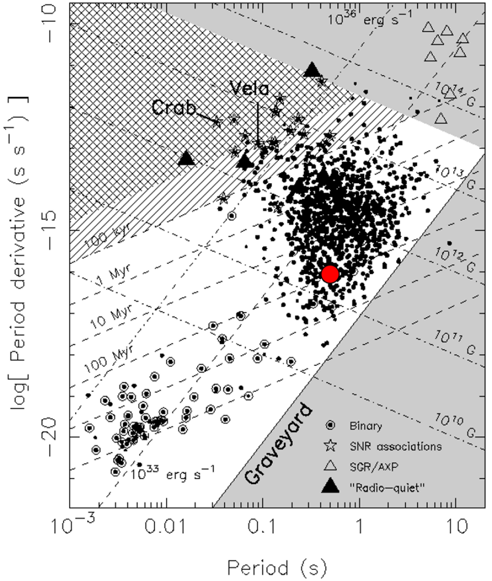
Figure 6.5: A plot of spin period against rate of spin-down for the population of all radio pulsars, generally referred to as a $P$–$\dot{P}$ diagram. Diagonal lines indicate the estimated age and surface magnetic field strength of a typical radio pulsar at any given position on the diagram. Any pulsars to the right of the ‘graveyard’ line on this plot are expected to be inactive in the radio, whereas objects to the left are expected to be observable as radio pulsars (e.g. van den Heuvel,, 1993). The position of the Bursting Pulsar, estimated from its surface field strength and spin period, is shown in red; well outside of the pulsar graveyard. Figure adapted from Lorimer and Kramer, (2004), and is accurate as of the time of its first publication.

6.3.1 Comparison with other Objects

In addition to the Bursting Pulsar, several additional sub-10 Hz accreting X-ray pulsars have been discovered (e.g. GX 1+4 and 4U 1626-67, Lewin et al.,, 1971; Rappaport et al.,, 1977). The reason behind the slow spins of these objects is poorly understood, but a number of these systems have been seen to undergo ‘torque reversal’ events, during which $\dot{P}$ switches sign (e.g. Chakrabarty et al., 1997b, ; Chakrabarty et al., 1997a, ). In some sources, the magnitude of the spin-down during an event is of the same order of magnitude as the preceding period of spin-up, resulting in little or no net spin change. Torque reversal events occur irregularly, but the recurrence timescale varies between objects from weeks to decades (e.g. Bildsten et al.,, 1997).

The slow accreting pulsar Vela X-1 has been found to show an anticorrelation between hardness and intensity (Kreykenbohm et al.,, 2008), whereas I find a strong positive correlation between these parameters in the Bursting Pulsar during periods of Structured Bursting (Figure 6.3). This significant spectral difference, combined with the other phenomenological differences between these objects reinforces the idea that the Bursting Pulsar exists in a very different physical state from the other known slow accreting pulsars.

Given that the Bursting Pulsar has a strongly stripped stellar companion (Bildsten and Brown,, 1997), a high magnetic field and shows significant spin-up during outburst (e.g. Finger et al., 1996b, ; Sanna et al., 2017c, ), it is difficult to explain its low spin by suggesting the system is young or that the angular momentum transfer is inefficient. Rappaport and Joss,, 1997 suggest that the magnetic field and spin could be explained if much of the mass transfer in the system occurred before the primary became a neutron star, but they note that this scenario is inconsistent with the low mass of the donor star.

Torque reversal events in the Bursting Pulsar (similar to those seen in other slow accreting pulsars, e.g. Bildsten et al.,, 1997) could explain why the pulsar has failed to reach a spin rate on par with TMSPs. Although no torque reversal event has been reported from the Bursting Pulsar, it is feasible that the recurrence timescale of such an event is longer than the $\sim 20$ years for which the object has been studied (this is consistent with the recurrence timescales seen in other slow accreting pulsars). The discovery of torque reversal in the Bursting Pulsar would strongly link it with the other known slow accreting pulsars.

The Rapid Burster is often compared to the Bursting Pulsar due to the presence of regular Type II X-ray bursts in both objects (e.g. Lewin et al.,, 1996). This system also contains an accreting neutron star. Iaria et al.,, 2018 have suggested that the vast majority of matter transferred in this system is ejected, similar to a scenario suggested by Degenaar et al., 2014a, to explain high-velocity winds from the Bursting Pulsar. However it remains unclear why the Rapid Buster does not show pulsations or display the ‘hiccup’ behaviour seen in the Bursting Pulsar.

6.4 Conclusion

The Bursting Pulsar has a spin rate $\sim 2$ orders of magnitude less than previously known TMSPs, and a magnetic field $\sim 2$ orders of magnitude stronger, but it still shows lightcurve, timing and spectral behaviour which are remarkably similar to TMSPs. This raises the exciting prospect of exploring the physics of TMSPs in a previously unexplored physical regime. If the Bursting Pulsar itself is a transitional pulsar, it should emit radio pulsations during X-ray quiescence. Future detections of radio pulsations from this object would unambiguously confirm it as a transitional pulsar.

Chapter 7 Discussion

These thoughts are constructive criticisms. Pyramidical. I try to suppress these thoughts, but they leak out…

George Saden – Zardoz

In Chapters 4 and 5 I discuss new ways of classifying variability in the unusual LMXBs IGR J17091 and the Bursting Pulsar. I use the new classification frameworks I have created to compare these objects with the similar LMXBs GRS 1915 and the Rapid Burster. While I find a number of similarities between these objects, I also highlight a number of differences. For example, I find that the spectral evolution during variability in IGR J17091 is very different to in GRS 1915, and the bursts in the Bursting Pulsar evolve in a very different way to those seen from the Rapid Burster.

A common theme throughout the work presented in this thesis is that the variability in these unusual objects is even more complex than had previously been thought. Application of Occam’s razor (of Ockam,, 1495) suggests that the similar variability from these objects is generated by similar physics, but I have found that it is difficult to unify the diverse behaviours of these unusual systems. I also compare the four objects that I focus on with other unusual XRBs such as Terzan 5 X-2 and, in Chapter 6, TMSPs. In this chapter I further discuss the relationships between these seemingly disparate objects, and how my findings fit in to the more general picture of accretion in these extreme and bizarre systems.

7.1 General Observations

7.1.1 Variability Evolution throughout an Ouburst

One feature common to at least 3 of the unusual LMXBs discussed in this thesis is that variability changes in a predictable way over the course of an outburst. This effect is most apparent in the results I present in Chapter 5, where I discuss an evolution of bursting which is observed in both the 1996 and 1997 outbursts of the Bursting Pulsar:

• Normal Bursts and Minibursts begin to occur shortly after the peak of each outburst.

• Bursting shuts off entirely when the persistent intensity of the source decreases below $\sim 0.1$ Crab.

• The persistent flux of the system increases in a rebrightening event, at which point Mesobursts begin to occur.

• Mesobursts evolve into Structured Bursting.

A predictable evolution of variability throughout an outburst has also been identified in the Rapid Burster (e.g. Bagnoli et al.,, 2015). In this system, Type II bursts near the start of each outburst are Eddington-Limited and persist for $\sim 100$s of seconds (see e.g. the upper panel of Figure 5.22). As the outburst evolves, these bursts become shorter, fainter and more sharply peaked (see e.g. the lower panel of Figure 5.22). This evolution is qualitatively very different from the evolution of variability seen in the Bursting Pulsar. However, the fact that bursting in both objects changes in a predictable way throughout each outburst shows that bursting in both objects is dependent on the accretion rate in the system and on the state of its accretion disk.

There is also some evidence of an evolution of the variability displayed by IGR J17091. In Figure 4.2 I show a number of lightcurves of the 2011 outburst of IGR J17091, highlighting when in the outburst each of our 9 variability classes was observed. Although the evolution between classes apparently not as strict as in the Bursting Pulsar, it is easy to identify a number of patterns in the data, such as:

• Class I only occurs near the start of the outburst, within 25 days of the onset of variability.

• Class II only occurs during two dips in the persistent flux to a level of $\sim 20$ mCrab.

• Class VII only occurs while the persistent flux of IGR J17091 is in a narrow band centred on $\sim 70$ mCrab.

It is unclear whether a similar evolution occurs during the 2016 outburst of IGR J17091, as a variability population study for this outburst has not yet been performed. However these results from the 2011 outburst suggest that variability in IGR J17091 also depends strongly on the accretion rate and the state of the disk, as it is in the Rapid Burster and the Bursting Pulsar, and therefore variability should evolve in a predictable way over the course of each outburst.

7.1.2 Criteria for Exotic Variability

As we show in Figure 7.1, the 2016 outburst of IGR J17091 displayed similar variability to that which it showed in 2011 (e.g. Reynolds et al.,, 2016), meaning that variability was not unique to the source’s 2011 outburst. Additionally Type II bursting has been seen in the 1996, 1997 and 2014 outbursts of the Bursting Pulsar, and the Rapid Burster goes into outburst regularly every $\sim$100–200 days and always displays Type II bursts. Therefore 3 of the 4 objects I discuss in this thesis have produced their characteristic variable behaviour during multiple separate outbursts. This observation strongly suggests that the ability to produce such variability is a property of the system rather than of an individual outburst. In these systems some set of parameters, which persist between outbursts, are just right to allow these exotic types of variability to occur.

Figure 7.1: 0.3–10 keV Swift/XRT lightcurve of IGR J17091-3624 during its 2016 outburst. The black bar shows the typical size of errors. This lightcurve shows Class III variability, which I identify in the 2011 outburst of this source and describe in Section 4.2.2.

Compact objects are relatively simple, and they can be well-defined with only a few parameters:

• The type of compact object (neutron star or black hole).

• Mass.

• Spin and rate of change of spin.

• Radius.

• Magnetic Field Strength.

Where the last two parameters only apply if the object is a neutron star. In addition to these, one only has to describe the companion star (mass, mass loss rate, spectral type etc.), the parameters of the system orbit (eccentricity, semi-major axis, inclination and misalignment from the spin axes of both stars) and the mass transfer rate to fully describe an LMXB system. Due to this relative simplicity, there are not many candidates for parameters which govern the existence of exotic variability.

GRS 1915+105 contains the highest mass black hole confirmed in an LMXB ($12.4\pm 2.0$ M_⊙, Reid et al.,, 2014), although many other LMXBs are believed to contain black holes with comparable masses (e.g. V404 Cyg, Shahbaz et al.,, 1994). The black hole in GRS 1915 also has a very high spin, with a spin parameter of $0.98\pm 0.01$ (Miller et al.,, 2013), but a number of other XRBs are also believed to harbour near-maximal spin black holes (see e.g. Fragos and McClintock,, 2015). Therefore it seems unlikely that mass or spin alone provide the criteria for GRS 1915-like variability.

Lense-Thirring precession in the disk, a frame-dragging effect caused by the misalignment of the orbital and spin axes of the compact object, has been used to explain some of the variability seen in LMXBs (e.g. Stella and Vietri,, 1998). However, the timescale of the variability this generates is no slower than $\sim 0.1$ s (Ingram et al.,, 2009), too fast to be linked with the $\lesssim 0.1$ Hz variability seen from GRS 1915. Instead the other parameters on the list, or a combination thereof, must be the determining factors in whether or not an object can display exotic variability.

GRS 1915 has a very long orbital period of $\sim 30$ days (Neil et al.,, 2007), and this is believed to result in it having the largest accretion disk of all known X-ray binaries. This likely explains how GRS 1915 has been in outburst for such a long period of time ($\gtrsim 20$ years, compared to the $\lesssim 2$ year outbursts seen in most black hole LMXBs). The orbital periods of IGR J17091 and the Rapid Burster are unknown, but the Bursting Pulsar also has a relatively long orbital period of 11.8 days (e.g. Finger et al., 1996b, ), suggesting that a large disk may also be a factor in the generation of exotic variability.

Another property to consider is the magnetic field strength in the disk. Although astrophysical black holes do not have a magnetic field, magnetic fields in a black hole can still arise from one of two sources:

• The field of the system’s donor star, including field lines advected into the disk by accretion.

• The movement of ionised material within the disk.

The presence of such a magnetic field may be able to stabilise an accretion disk against the instabilities described in Section 2.2.3 (e.g. Sa̧dowski,, 2016. Sa̧dowski, calculates the minimum magnetic field strength which, when threaded through a radiation-dominated disk undergoing the instability described by Shakura and Sunyaev, (1976), would be able to stabilise the disk. Assuming that such a field in an LMXB is provided by the companion star, they find that this minimum value in an LMXB depends mostly on the luminosity of the system and the mass of the compact object. They estimate the value of the minimum stabilising field strength in a number of black hole X-ray binaries, and find that the field required to stabilise GRS 1915 is $\sim 5.7\times 10^{23}$ G cm²; this is over twice as large as the second highest value they find for an LMXB ($1.9\times 10^{23}$ G cm² for XTE J1550-564). This high value is due to the large black hole mass in GRS 1915, and the fact that this black hole accretes at a near-Eddington rate and, thus, a high luminosity. In this picture, therefore, GRS 1915-like variability may simply be a manifestation of the Shakura and Sunyaev, (1976) instability which is suppressed in most LMXBs. One could test the viability of this scenario by calculating the minimum stabilising field for IGR J17091. Unfortunately at time of writing the companion star to IGR J17091 has not been conclusively identified, and the mass and distance (and hence luminosity) of the system remain poorly constrained.

It is worth noting that the scenario suggested by Sa̧dowski, (2016) by itself is unable to account for Type II bursts as, in these systems, the neutron star is able to provide more than enough magnetic flux to stabilise the inner disk in the scenario of Sa̧dowski,. However, the scenario of Sa̧dowski, does not take into account the effects of the magnetic disruption of the inner disk, nor does it account for any effects caused by the disk’s interaction with the rapidly spinning neutron star magnetic field.

7.1.3 Evidence of System Memory

Another notable observation from these objects is that variability in both GRS 1915 and IGR J17091 falls into a discrete set of variability classes. In both objects, a variability class could be observed on one day, not be observed for weeks and then reappear in a later observation. Somehow, the physics that governs variability in these systems only permit the system to occupy one of a discrete set of variability classes. In Figure 7.1 I show evidence that at least one of the variability classes I identified in the 2011 outburst of IGR J17091 occurred again in 2016. This suggests that GRS 1915-like systems are somehow able to ‘remember’ which variability classes they can occupy, and that this memory persists between outbursts. This in turn means that, in addition to determining whether or not GRS 1915-like variability can occur, the simple parameters that define a black hole LMXB also determine which classes of GRS 1915-like variability can occur.

In Section 4.3.1, I report that two of the classes of variability I find in IGR J17091 (Classes VII and VIII) are unlike anything which has ever been seen in GRS 1915 (see also Table 4.5). This leads to one of three possibilities:

• Class VII and VIII-like variability has occurred in GRS 1915 since its discovery, but coincidentally we have never observed it. As GRS 1915 has been observed extensively during its ongoing $\gtrsim 20$ year-long outburst, this is unlikely to be true.

• Class VII and VIII variability preferentially occurs during a specific disk configuration which occurs at a specific point in the evolution of an outburst, and GRS 1915 is not currently in this state.

• Some set of system parameters in IGR J17091 are different from in GRS 1915 in such a way that many variability classes can appear in both objects, but a small set of different variability classes are permitted in each object.

The final possibility is of great interest. Future observations of IGR J17091 will aim to better constrain the parameters that define the system. If these parameters are then compared to the already well-constrained parameters of GRS 1915, then we may be able to learn exactly which physical properties of the system govern which set of variability classes can be displayed.

There is also evidence of some degree of system memory in the Type II bursting systems. The near-identical evolutions of variability in the 1996 and 1997 outbursts of the Bursting Pulsar indicate that the factors governing this evolution persist between outbursts in this object as well.

The Normal Bursts and Minibursts of the Bursting Pulsar, which I describe in Sections 5.2.3 and 5.2.4 respectively, also provide evidence of system memory in the Bursting Pulsar. Both types of burst display a number of similar features and they occur interchangeably during the same period of each outburst, leading to the possibility that they are generated by the same physical instability. As I show in Figure 5.23, Minibursts and Normal Bursts fall into two clear populations when plotted by their amplitudes: we find no Normal or Minibursts with fluences between $\sim 10^{4}$ and $\sim 10^{5}$ 2–60 keV PCA counts. Due to the large number of Minibursts and Normal Bursts observed in my study, it is highly likely that this gap is real. Observations of future outbursts of the Bursting Pulsar will allow us to see whether this fluence gap always spans the same range, or whether this gap changes between outbursts as a function of the longer-term evolution of the system.

7.2 IGR J17091 vs. the Bursting Pulsar: A Comparison

It is clear that there are a number of significant similarities between objects which display Type II bursts and GRS 1915-like variability. What remains unclear is how, if at all, the physics of GRS 1915-like variability and Type II bursting are related to each other. Many of the models proposed to explain GRS 1915-like variability and Type II bursts rely on similar viscous disk instabilities (see Sections 2.3.1 and 2.4.1), and the discovery of GRS 1915-like patterns in lightcurves of the Rapid Burster strongly suggests a link between these two classes of object (Bagnoli and in’t Zand,, 2015).

Historically, the Bursting Pulsar has been considered a ‘twin’ system to the Rapid Burster (however, see Lewin et al.,, 1996), but the many differences I find between these object calls this comparison into doubt. In Chapter 6 I consider the possibility that some of the bursting seen in the Bursting Pulsar is a result of the object being similar to TMSPs. In this section, I consider the alternative possibility that bursting in the Bursting Pulsar is instead a manifestation of GRS 1915-like variability.

7.2.1 Variability Classes and Burst Classes

A number of disparate features in data from the Bursting Pulsar are at least superficially similar to behaviours I identify in IGR J17091-3624. In Figures 7.2 and 7.3 I identify features in IGR J17091 data which resemble Normal Bursts and Structured Bursting in the Bursting Pulsar. As discussed in Section 7.1, there are a number of system similarities between IGR J17091 and the Bursting Pulsar, so perhaps the similarities in their lightcurves should not be surprising. However, any attempt to compare Bursting classes in the Bursting Pulsar with variability classes in IGR J17091 encounters a number of difficulties:

Figure 7.2: Lightcurves from GRS 1915, IGR J17091 and the Bursting Pulsar, each showing heartbeat-like variability over timescales of 10s to 1000s of seconds. Black bars indicate average error in each case. GRS 1915 and IGR J17091 data taken from RXTE/PCA, Bursting Pulsar data taken from Chandra.

Figure 7.3: Lightcurves from GRS 1915, IGR J17091 and the Bursting Pulsar, each showing a Structured Bursting-like variability over timescales of 10s to 100s of seconds. Black bars indicate average error in each case. Data taken from RXTE/PCA.

• Variability in IGR J17091 is likely caused by some instability in the inner, radiation-dominated part of its accretion disk. The inner region of the disk in the Bursting Pulsar is dominated by magnetic pressure rather than radiation pressure, leading to different possible instabilities.

• IGR J17091 can evolve from one variability class to another quickly (over timescales of $\lesssim 1$ day), whereas Normal Bursts and Minibursts occur continuously in the Bursting Pulsar for many weeks during each outburst.

• IGR J17091 shows complex variability from the peak of each outburst until the time it enters the low/hard state, whereas the Bursting Pulsar shows a large gap with no bursts between the end of Normal Bursts and the onset of Mesobursts.

• All complex variability in IGR J17091 occurs over a relatively narrow range of luminosities (a factor of $\sim 3$, see e.g. Figure 4.2). Bursting in the Bursting Pulsar occurs at luminosities spanning more than an order of magnitude.

• All complex variability in IGR J17091 occurs during the main high-soft portion of its outbursts, whereas Mesobursts and Structured Bursting are seen during rebrightening events in the Bursting Pulsar.

Because of these differences, it is unlikely that Burst Classes in the Bursting Pulsar can be considered as being generated by the exact same phenomenon as variability classes in IGR J17091. Some of the apparent similarities between the phenomena could instead be explained by phenomenological limit cycles common to both. For example, if both Class IV variability and Normal Bursts involve the filling and depletion of a portion of the inner part of the accretion disk, then it is to be expected that the flares in both types of variability have similar morphologies.

7.2.2 Structured Bursting

Structured Bursting in the Bursting Pulsar on its own can also be compared with the variability classes observed in IGR J17091. As discussed in Section 5.2.6, and shown in Figure 5.20, Structured Bursting is a highly variable phenomenon. Like variability in IGR J17091, Structured Bursting in the Bursting Pulsar consists of flares, flat-bottomed dips in flux and periods of seemingly unstructured noise. As such, an alternative hypothesis to the ‘hiccup’ scenario presented in Chapter 6 is that Structured Bursting is an example of GRS 1915-like variability manifesting in a neutron star LMXB.

There are a number of problems with simply equating Structured Bursting with GRS 1915-like variability classes. Variability in GRS 1915 and IGR J17091 shows hysteresis in hardness-intensity diagrams, indicating a finite lag between hard and soft emission from the source. However no such hysteresis exists in Structured Bursting from the Bursting Pulsar: as we show in Figure 6.3, hardness and intensity simply correlate during periods of Structured Bursting. In addition to this, the source intensities involved in GRS 1915-like variability and Structured Bursting are very different; GRS 1915 is a near-Eddington source, but Structured Bursting in the Bursting Pulsar occurs at a luminosity no greater than 0.5% of its Eddington Luminosity.

If however Structured Bursting and GRS 1915-like variability are the same phenomenon, then these issues may be resolved in a number of ways. While the hard lag in GRS 1915 is positive in every variability class, I find that its sign can vary in different variability classes in IGR J17091. Therefore, it is feasible to imagine a GRS 1915-like system in which this lag is always close to zero, resulting in a simple correlation between rate and hardness in a HID rather than a hysteretic loop. Notably, the GRS 1915-like lightcurves reported from the Rapid Burster (Bagnoli and in’t Zand,, 2015) also show no hysteretic loops.

The apparent different luminosity regimes of GRS 1915 and the Bursting Pulsar can be resolved if GRS 1915-like variability does not require near-Eddington accretion. I discuss this possibility in Section 7.1.2. The Rapid Burster is known to accrete at $\sim 20$% of its Eddington Limit, and I find that IGR J17091 likely accretes at 5–33% of its Eddington Limit (Section 4.3.5), so these systems set possible precedents for GRS 1915-like variability in systems which are not near-Eddington limited.

To further investigate the similarities between GRS 1915-like variability and Structured Bursting, the natural next step would be to perform phase-resolved spectroscopy on Structured Bursting data. Archival data of Structured Bursting from the Bursting Pulsar only exists from the 1996 and 1997 outbursts of the source, as no observations were taken during the latter stages of its outbursts in 2014 or 2017. The Bursting Pulsar is a faint source during periods of Structured Bursting, and is in a crowded region of the sky populated by many other X-ray sources, and such a study is difficult to perform on data from instruments launched before 1996. As such, it remains unclear whether Structured Bursting is a neutron star manifestation of GRS 1915-like variability or whether it is a manifestation of ‘hiccup’ accretion as I suggest in Chapter 6.

7.3 Future Research

A number of recently-launched and planned satellites have sensitivities, collecting areas and energy resolutions which exceed those of the instruments I use in this study. For example, the currently operational Neutron Star Interior Composition Explorer (NICER, Gendreau et al.,, 2012) has a 0.5–10 keV X-ray sensitivity around 30 times greater than that of RXTE, with an energy resolution comparable to XMM-Newton and Chandra. The European Advanced Telescope for High Energy Astrophysics (ATHENA, Johnson et al.,, 1995), planned for launch in the 2030s, is expected to have a sensitivity around 2 orders of magnitude greater than XMM-Newton or Chandra. This generation of highly sensitive instruments will allow us to perform phase-resolved spectroscopy of variability from fainter objects, such as IGR J17091 and the Bursting Pulsar during periods of Structured Bursting.

A phase-reolved spectroscopic study of the variability classes in IGR J17091 will allow us to identify the physical changes in the accretion disk that occur during each class. This study will be able to be compared to the phase-resolved spectral study of GRS 1915 by Neilsen et al., (2011), allowing us to further understand the similarities and differences between these two systems.

Phase-resolved spectral studies will also be possible to perform on the fainter classes of bursting seen in the Bursting Pulsar. These will allow us to understand the physical mechanisms underlying each class of burst, in particular identifying which bursts if any are a result of thermonuclear burning on the surface of the neutron star. This information will allow us to better understand whether bursting in the Bursting Pulsar is a manifestation of the same instabilities seen in GRS 1915 and IGR J17091, and will allow us to understand where all of these systems fit in a picture of accretion disk instability as a whole.

Chapter 8 Conclusions

And this goes on and on and back and forth for 90 or so minutes, until it just sort of… ends.

Dennis Reynolds – It’s Always Sunny in Philadelphia

In this thesis, I have presented the results of phenomenological studies of the X-ray variability seen in two unusual LMXBs: IGR J17091-3624 and GRO J1744-28 (the “Bursting Pulsar”). I have analysed these results in the context of previous studies of variability in GRS 1915+105 and MXB 1730-335 (the “Rapid Burster”), systems which are often compared to IGR J17091 and the Bursting Pulsar respectively. In doing so I have discovered a number of new similarities and differences between these objects. On the back of this analysis, I have evaluated the physical models and scenarios which have been proposed to explain the variability in these objects. In doing so, I have brought us closer to an understanding of the accretion physics that underlies this exotic behaviour.

In Chapter 4, I have presented a new set of variability classes to describe IGR J17091: these classes are analogous to, but independent from, the classes presented by Belloni et al., (2000) to describe GRS 1915. Comparing my set of variability classes to those of Belloni et al.,, I found a number of variability classes which are only seen in one of the two objects, as well as a number of types of variability which are seen in both. When studying the spectral timing properties of both objects, I found another significant difference: while hard photons lag soft photons in every variability class of GRS 1915, the sign of this lag varies from class to class in IGR J17091. This finding rules out any physical picture in which the hard lag is caused by a corona reacting to changes in the flux from the disk, instead suggesting that the hard lag is generated by a spectral change in the emission from the disk.

In Chapter 5, I have presented a new set of classifications for Type II-like X-ray bursts from the Bursting Pulsar. In doing so, I have discovered previously unreported bursting behaviour in the late stages of outbursts of the Bursting Pulsar, namely ‘Mesobursts’ and ‘Structured Bursting’. I find that Mesobursts may be a manifestation of quasi-stable thermonuclear burning on the surface of the neutron star; a phenomenon which has long been predicted to occur on the Bursting Pulsar but which has never been conclusively identified (e.g. Bildsten and Brown,, 1997). There are similarities between lightcurves of Structured Bursting and the lightcurves of another form of quasi-stable nuclear burning predicted by Heger et al., (2007). However I find that at least one Mesoburst occured during a period of Structured Bursting without disrupting it, suggesting that Structured Bursting is non-nuclear in nature. Instead, in Chapter 6 I have identified similarities between Structured Bursting and variability seen in Transitional Millisecond Pulsars. This raises the possibility that Structured Bursting is a manifestation of ‘hiccup’ accretion; spasmodic accretion onto a neutron star caused by small perturbations of its magnetospheric radius near the boundary of the propeller regime.

From a phenomenological standpoint, I find that the variability seen in IGR J17091 and the Bursting Pulsar is generally even more complex than previously thought. IGR J17091 and the Bursting Pulsar have often been considered ‘twin systems’ of GRS 1915 and the Rapid Burster respectively, but I find a number of differences between each pair of twins which makes such a simple picture seem unlikely. Variability in GRS 1915 has traditionally been thought to be tied to its near-Eddington accretion rate; however, I find that IGR J17091 likely accretes at $\lesssim 33$% of its Eddington Limit. The Rapid Burster shows Type II bursts which transition smoothly between 2 classes over the course of an outburst, whereas I find that bursts in the Bursting Pulsar can be described in no less than 4 classes which take place at different periods of each outburst. Rather than suggesting that these pairs of objects are unrelated, I suggest that further study of their differences will lead to better understanding of the physics behind the instabilities that they present.

In Chapter 7 I discuss the relationship between GRS 1915-like variability and Type II X-ray bursts. While there are a number of problems with assuming that these two types of variability are the same, I find a number of similarities between them that suggest at least some of the physics underlying these phenomena are similar. Finally, I suggest that phase-resolved spectral studies by the next generation of space telescopes will allow us to fully understand the relationships, or lack thereof, between these four enigmatic objects.

I also present a number of results unconnected to the variability seen in these objects. In Chapter 4 I provide new constraints on the distance of IGR J17091-3624 and the mass of its black hole, and I also present the first INTEGRAL detection of the object above 150 keV. Additionally in Chapters 4 and 5 I report the discovery of ‘re-flares’ in the tails of outbursts in both IGR J17091 and the Bursting Pulsar. I have also created a number of algorithms to identify bursts or flares, and to ‘fold’ datasets which show repeating variability with a non-constant frequency (Chapter 3). These are encoded as part of my own suite of computational tools to analyse X-ray data (PANTHEON, see Appendix D).

In conclusion, the work I present in this thesis provides a comprehensive framework for future study of variability in IGR J17091 and the Bursting Pulsar. Using this framework, I have been able to rule out a number of models and physical scenarios which have been proposed to explain the behaviour seen in these systems. Further studies of the key properties of these systems will allow us to better understand the exotic instabilities which can be present in accretion disks and, as such, improve our knowledge of the physics of accretion in general.

Appendix A Model-Independent Classification of each Observation of IGR J17091-3624

In Table A.1, I present observation IDs, and orbit IDs, for every RXTE observation and observation segment that was used in my study of variability in IGR J17091-3624 (Chapter 4). Note that not all of every observation was used; in many cases, large spikes caused by PCA PCUs switching off or on rendered $\sim 100$ s unusable. As these often occurred very close to the beginning or end of an observation segment, small sections of data before or after these spikes was also sometimes discarded. Every observation segment is presented along with the variability class assigned to it by this study.

Table A.1: Here is listed the Observation IDs for every RXTE observation that was used in my analysis of variability in IGR J17091-3624, along with the variability class which has been assigned to it. Orb. is the orbit ID (starting at 0) of each observation segment, Exp. is the exposure time in seconds and X is the prefix 96420-01. This table is continued overleaf in Tables A.2-A.4.

MJD	OBSID	Orb.	Class	Exp.	MJD	OBSID	Orb.	Class	Exp.
55622	X-01-00	0	I	1840	55643	X-04-01	0	III	1190
55622	X-01-000	0	I	3480	55644	X-04-03	0	III	2903
55622	X-01-000	1	I	1656	55645	X-05-02	0	I	3578
55622	X-01-000	2	I	3384	55647	X-05-00	0	IV	2872
55622	X-01-000	3	I	3400	55647	X-05-000	0	IV	3472
55622	X-01-000	4	I	3384	55647	X-05-000	1	IV	3520
55623	X-01-01	0	I	1240	55647	X-05-000	2	IV	3512
55623	X-01-01	1	I	752	55647	X-05-000	3	IV	3520
55623	X-01-01	2	I	992	55647	X-05-000	4	IV	3512
55623	X-01-01	3	I	1184	55647	X-05-000	5	IV	648
55623	X-01-01	4	I	1056	55649	X-05-03	0	IV	2409
55623	X-01-010	0	I	2080	55650	X-05-01	0	IV	1473
55623	X-01-010	1	I	1832	55651	X-05-04	0	IV	2954
55623	X-01-010	2	I	1648	55653	X-06-00	0	IV	2723
55623	X-01-010	4	I	1424	55654	X-06-01	0	IV	3388
55623	X-01-010	5	I	400	55656	X-06-02	0	IV	2908
55623	X-01-02	0	I	3056	55657	X-06-03	0	V	1842
55623	X-01-02	1	I	2792	55661	X-07-00	0	V	1754
55623	X-01-02	2	I	2432	55662	X-07-01	0	V	3365
55623	X-01-020	0	I	3456	55663	X-07-02	0	V	3373
55623	X-01-020	1	I	3464	55666	X-08-00	0	V	3338
55623	X-01-020	2	I	3512	55669	X-08-01	0	V	3368
55623	X-01-020	3	I	3520	55670	X-08-03	0	VI	2489
55623	X-01-020	4	I	3512	55671	X-08-02	0	VI	2609
55623	X-01-020	5	I	464	55673	X-09-03	0	VI	1011
55624	X-02-00	0	I	1758	55674	X-09-00	0	VI	1386
55626	X-02-01	0	I	1380	55675	X-09-05	0	IX	1148
55628	X-02-02	0	I	3305	55676	X-09-06	0	VI	3540
55630	X-02-03	0	I	1876	55677	X-09-01	0	V	1676
55632	X-03-00	0	I	1712	55678	X-09-04	0	V	2090
55634	X-03-01	0	III	3590	55679	X-09-02	0	V	2306
55639	X-04-00	0	IV	3099	55680	X-10-02	0	V	952
55642	X-04-02	0	IV	2972	55681	X-10-00	0	V	3725

Table A.2: A continuation of Table A.1. This table is continued overleaf in Tables A.3 and A.4.

MJD	OBSID	Orb.	Class	Exp.	MJD	OBSID	Orb.	Class	Exp.
55682	X-10-03	0	V	1157	55720	X-15-04	0	IV	1486
55684	X-10-01	0	III	1504	55721	X-15-05	0	IV	1500
55686	X-10-04	0	III	1127	55722	X-16-00	0	IV	900
55686	X-10-05	0	II	2179	55723	X-16-01	0	III	1004
55687	X-11-00	0	II	3537	55724	X-16-02	0	II	1923
55688	X-11-01	0	II	1153	55725	X-16-03	0	II	1919
55690	X-11-02	0	II	1408	55726	X-16-04	0	III	1935
55691	X-11-03	0	II	886	55727	X-16-05	0	II	730
55692	X-11-04	0	II	3566	55728	X-16-06	0	II	1953
55693	X-11-05	0	II	1817	55729	X-17-00	0	II	2735
55694	X-12-00	0	II	2761	55730	X-17-01	0	II	3556
55695	X-12-01	0	II	1374	55731	X-17-02	0	II	3605
55695	X-12-02	0	II	2041	55732	X-17-03	0	II	1647
55696	X-12-03	0	II	1456	55733	X-17-04	0	II	1459
55698	X-12-04	0	II	1916	55734	X-17-05	0	III	1736
55698	X-12-05	0	II	3139	55735	X-17-06	0	III	3653
55700	X-12-06	0	II	1189	55736	X-18-00	0	III	2317
55701	X-13-00	0	II	1214	55737	X-18-01	0	IV	1387
55702	X-13-01	0	II	980	55738	X-18-02	0	V	1291
55704	X-13-02	0	II	732	55739	X-18-03	0	V	2178
55705	X-13-03	0	III	1217	55740	X-18-04	0	V	1478
55706	X-13-04	0	III	1161	55741	X-18-05	0	VII	782
55707	X-13-05	0	IV	2763	55743	X-19-00	0	VII	1412
55708	X-14-00	0	IV	1188	55744	X-19-01	0	VIII	1938
55709	X-14-01	0	IV	3342	55745	X-19-02	0	VII	2172
55710	X-14-02	0	IV	1094	55747	X-19-03	0	VIII	1691
55712	X-14-03	0	IV	1404	55748	X-19-04	0	VI	1283
55713	X-14-04	0	V	871	55749	X-19-05	0	VIII	1417
55714	X-14-05	0	V	1311	55751	X-20-05	0	VI	1726
55715	X-15-00	0	IV	1241	55752	X-20-01	0	VIII	1079
55716	X-15-01	0	IV	1262	55753	X-20-02	0	VIII	1433
55717	X-15-02	0	III	1557	55754	X-20-03	0	VII	1122
55718	X-15-03	0	III	1334	55756	X-20-04	0	VIII	1486

Table A.3: A continuation of Table A.1. This table is continued overleaf in Table A.4.

MJD	OBSID	Orb.	Class	Exp.	MJD	OBSID	Orb.	Class	Exp.
55757	X-21-00	0	VIII	3372	55790	X-25-05	0	V	1473
55758	X-21-01	0	VIII	3383	55791	X-25-06	0	V	922
55759	X-21-02	0	VI	1938	55792	X-26-00	0	V	2336
55761	X-21-04	0	VII	1497	55794	X-26-01	0	V	1385
55762	X-21-05	0	VII	1548	55795	X-26-02	0	VIII	1458
55763	X-21-06	0	VII	2202	55796	X-26-03	0	VI	1325
55764	X-22-00	0	VII	1682	55798	X-26-04	0	VI	2075
55765	X-22-01	0	VII	1221	55799	X-27-00	0	VI	1396
55766	X-22-02	0	V	720	55800	X-27-01	0	VI	2684
55767	X-22-03	0	V	1801	55801	X-27-02	0	VI	1016
55768	X-22-04	0	VIII	1983	55802	X-27-03	0	VI	1179
55769	X-22-05	0	VIII	999	55803	X-27-04	0	VI	1304
55770	X-22-06	0	VIII	667	55805	X-27-05	0	VI	1663
55771	X-23-00	0	VIII	2075	55806	X-28-00	0	VI	1456
55772	X-23-01	0	VII	3385	55808	X-28-01	0	VIII	577
55773	X-23-02	0	VII	2218	55810	X-28-02	0	VI	1251
55774	X-23-03	0	V	1811	55811	X-28-03	0	VI	2000
55775	X-23-04	0	V	3356	55813	X-29-00	0	VIII	1309
55776	X-23-05	0	V	2603	55819	X-29-04	0	VIII	1686
55777	X-23-06	0	IV	912	55820	X-30-00	0	VI	1488
55777	X-23-06	1	IV	1544	55821	X-30-01	0	VI	1503
55778	X-24-00	0	IV	1309	55822	X-30-02	0	VI	1417
55779	X-24-01	0	IV	3599	55823	X-30-03	0	VI	1290
55779	X-24-02	0	IV	2013	55824	X-30-04	0	VI	1489
55782	X-24-03	0	V	1761	55825	X-30-05	0	VI	2581
55782	X-24-04	0	V	1725	55826	X-30-06	0	VI	2747
55784	X-24-05	0	V	3144	55827	X-31-00	0	VI	1559
55784	X-24-06	0	V	2591	55828	X-31-01	0	VI	2954
55785	X-25-00	0	V	2366	55829	X-31-02	0	IX	3005
55786	X-25-01	0	V	1804	55830	X-31-03	0	IX	1472
55787	X-25-02	0	V	1951	55830	X-31-03	1	IX	288
55788	X-25-03	0	V	1619	55831	X-31-04	0	IX	1586
55789	X-25-04	0	V	2601	55832	X-31-05	0	VI	3812

Table A.4: A continuation of Table A.1.

MJD	OBSID	Orb.	Class	Exp.	MJD	OBSID	Orb.	Class	Exp.
55833	X-31-06	0	IX	3675	55867	X-36-05	0	IX	1732
55834	X-32-00	0	IX	1217	55868	X-36-06	0	IX	1657
55835	X-32-01	0	IX	1445	55871	X-37-00	0	IX	815
55836	X-32-02	0	IX	1591	55871	X-37-02	0	IX	1460
55837	X-32-03	0	IX	2155	55872	X-37-03	0	IX	1683
55838	X-32-04	0	IX	2641	55873	X-37-04	0	IX	1402
55838	X-32-05	0	IX	2077	55874	X-37-05G	0	IX	1536
55840	X-32-06	0	IX	3392	55875	X-37-06	0	IX	1536
55840	X-32-06	1	IX	3512	55876	X-38-00	0	IX	1497
55840	X-32-06	2	IX	3934	55877	X-38-01	0	IX	1134
55840	X-32-06	3	IX	3880	55878	X-38-02	0	IX	1289
55840	X-32-06	4	IX	1896	55879	X-38-03	0	IX	1433
55841	X-33-00	0	IX	1188
55842	X-33-01	0	IX	855
55843	X-33-02	0	IX	1156
55845	X-33-04	0	IX	1713
55846	X-33-05	0	IX	934
55847	X-33-06	0	IX	717
55848	X-34-00	0	IX	1159
55849	X-34-01	0	IX	973
55851	X-34-02	0	IX	2261
55852	X-34-03	0	IX	1092
55853	X-34-04	0	IX	741
55856	X-35-00	0	IX	797
55857	X-35-01	0	IX	1912
55859	X-35-02	0	IX	200
55859	X-35-02	1	IX	1296
55860	X-35-03	0	IX	1372
55861	X-35-04	0	IX	836
55862	X-36-00	0	IX	1145
55863	X-36-01	0	IX	1322
55865	X-36-03	0	IX	1485
55866	X-36-04	0	IX	1795

Appendix B List of RXTE Observations of the Bursting Pulsar

In Table B.1 we present a table of all RXTE observations used in our study of burst evolution in the Bursting Pulsar. The prefixes A, B, C, D and E correspond to OBSIDs beginning with 10401-01, 20077-01, 20078-01, 20401-01 and 30075-01 respectively.

Obsid	Exp.	Date	Obsid	Exp.	Date	Obsid	Exp.	Date
A-01-00	3105	119	A-34-00	1831	213	A-59-00	1152	257
A-02-00	1655	117	A-35-00	2563	216	A-59-01	2203	257
A-03-00	6724	122	A-36-00	3683	219	A-59-02	768	257
A-03-000	2372	122	A-37-00	3446	215	A-60-00	1907	260
A-03-01	768	122	A-38-00	1536	217	A-60-01	3376	260
A-04-00	639	128	A-39-00	2317	218	A-60-02	1783	260
A-05-00	1990	129	A-40-00	1239	220	A-60-03	1559	260
A-06-00	1280	134	A-41-00	1363	221	A-61-00	3292	262
A-08-00	2431	142	A-42-00	2728	224	A-61-01	3035	262
A-09-00	640	138	A-43-00	2079	225	A-61-02	2013	262
A-10-00	2470	143	A-44-00	2076	226	A-62-00	2390	264
A-11-00	2381	148	A-45-00	2050	228	A-62-01	1703	264
A-12-00	3352	151	A-47-00	2687	232	A-62-02	2719	264
A-13-00	3480	155	A-48-00	2267	234	A-63-00	517	266
A-14-00	1839	158	A-49-00	35	236	A-63-01	3077	266
A-15-00	1595	161	A-50-00	3719	238	A-64-00	2381	268
A-16-00	3470	156	A-51-00	3590	240	A-64-01	3110	268
A-17-00	4481	164	A-52-00	2518	241	A-65-00	2003	270
A-18-00	384	171	A-53-00	3063	243	A-65-01	2744	270
A-19-00	128	172	A-55-00	3328	245	A-65-02	4331	270
A-20-00	2087	178	A-55-01	3395	245	A-66-00	2203	272
A-21-00	2711	181	A-55-02	2667	245	A-66-01	1723	272
A-22-00	2816	183	A-56-00	512	250	A-66-02	2533	272
A-22-01	2911	185	A-56-01	1280	250	A-67-00	395	274
A-23-00	1678	187	A-56-02	1664	250	A-67-01	3533	274
A-24-00	2509	189	A-56-03	1920	250	A-67-02	3466	274
A-25-00	2846	192	A-57-00	2432	250	A-68-00	1841	276
A-26-00	768	194	A-57-01	894	253	A-69-00	3659	278
A-27-00	2923	196	A-57-02	1408	253	A-70-00	2022	280
A-28-00	6839	199	A-57-03	1792	253	A-71-00	3474	283
A-29-00	3478	201	A-58-00	1024	255	A-72-00	5687	285
A-30-00	5906	203	A-58-01	1401	255	A-73-00	3109	287
A-31-00	6170	206	A-58-02	1679	255	A-74-00	1659	289
A-32-00	2712	209	A-58-03	1683	255	A-75-00	1798	291

Table B.1: A list of all RXTE observations of the Bursting Pulsar used in this study. Exposure is given in seconds, and date is given in days from MJD 50000. The prefixes A, B, C, D and E correspond to OBSIDs beginning with 10401-01, 20077-01, 20078-01, 20401-01 and 30075-01 respectively. This table is continued in Tables B.2-B.3

Obsid	Exp.	Date	Obsid	Exp.	Date	Obsid	Exp.	Date
A-76-00	1558	293	B-10-00	1009	482	C-11-00	2330	527
A-77-00	1738	295	B-11-00	2864	487	C-11-01	290	527
A-78-00	463	297	B-12-00	1847	489	C-11-02	2399	527
A-79-00	1024	299	B-13-00	2805	497	C-12-00	3345	534
A-80-00	5818	301	B-14-00	3741	499	C-12-01	2048	534
A-81-00	6898	303	B-15-00	384	501	C-13-00	1735	541
A-82-00	3537	306	B-16-00	768	503	C-13-01	1691	541
A-83-00	512	308	B-17-00	2399	509	C-14-00	3579	549
A-84-00	6361	310	B-18-00	2306	511	C-14-01	2785	549
A-85-00	10391	312	B-19-00	3477	516	C-15-00	7494	579
A-86-00	9232	314	B-20-00	1922	520	C-16-00	4941	562
A-87-00	3109	316	C-01-00	8200	389	C-16-01	671	561
A-88-00	6630	318	C-02-00	1408	400	C-16-02	1159	562
A-89-00	2569	320	C-02-01	896	401	C-17-00	3537	568
A-90-00	2209	323	C-02-02	512	401	C-18-00	2981	576
A-91-00	2317	325	C-03-00	3409	465	C-18-01	3103	576
A-92-00	2199	327	C-03-01	2635	466	C-19-00	3286	582
A-93-00	3720	331	C-03-02	2645	466	C-19-01	2893	582
A-94-00	3216	332	C-04-00	2620	478	C-19-02	470	582
A-95-00	9487	333	C-04-01	2956	477	C-20-00	3460	589
A-96-00	2627	337	C-04-02	2515	476	C-20-01	1126	589
A-97-00	3341	340	C-05-00	1421	484	C-21-00	3659	596
A-98-00	99	343	C-05-01	1995	484	C-21-01	2907	596
A-99-00	2783	345	C-05-02	2505	485	C-21-02	1086	596
A-99-01	1001	344	C-06-00	2770	492	C-22-00	1967	602
B-01-00	1664	467	C-06-01	2375	492	C-22-01	3086	602
B-02-00	1920	468	C-06-02	2203	492	C-22-02	1024	602
B-03-00	2982	469	C-07-00	1258	494	C-23-00	3697	607
B-04-00	3530	470	C-08-00	3305	505	C-23-01	3091	607
B-05-00	2025	472	C-08-01	777	505	C-24-00	1152	618
B-06-00	2677	473	C-09-00	1377	513	C-24-01	2300	618
B-07-00	3365	473	C-09-01	1536	513	C-24-02	1386	618
B-08-00	3113	475	C-10-00	1664	517	C-25-00	4069	626
B-09-00	2868	480	C-10-01	3796	518	C-25-01	1920	626

Table B.2: A continuation of Table B.1. This table is further continued in Table B.3.

Obsid	Exp.	Date	Obsid	Exp.	Date	Obsid	Exp.	Date
C-25-02	768	626	C-39-01	4690	723	D-19-00	3158	650
C-26-00	2071	633	C-40-00	3419	730	D-20-00	751	672
C-26-01	4043	633	C-40-01	3419	730	E-01-00	512	831
C-27-00	1792	638	C-40-02	896	764	E-02-00	1836	845
C-27-01	2495	638	C-41-00	5255	735	E-03-00	1871	859
C-27-02	3082	638	C-41-01	2387	735	E-04-00	1927	873
C-28-00	3454	644	C-41-02	1141	744	E-05-00	2088	889
C-28-01	1359	644	C-42-00	1476	744	E-06-00	2003	901
C-28-02	756	644	C-43-00	5277	764	E-07-00	1536	914
C-29-00	1535	652	C-44-00	6712	769	E-08-00	967	935
C-30-01	3435	658	D-01-00	2688	523	E-09-00	1598	949
C-31-00	1920	662	D-02-00	3469	525	E-10-00	1835	961
C-31-01	1152	662	D-03-00	3026	528	E-11-00	1741	975
C-31-02	1012	657	D-04-00	3050	531	E-12-00	1032	991
C-32-00	4646	678	D-05-00	3485	536	E-13-00	1231	1001
C-32-01	2803	678	D-06-00	1367	538	E-14-00	1608	1016
C-33-00	4334	747	D-07-00	3196	543	E-15-00	1712	1030
C-33-01	3534	748	D-08-00	2617	548	E-16-00	1440	1045
C-33-02	2957	748	D-09-00	2598	553	E-17-00	1888	1057
C-34-00	3477	687	D-10-00	4069	560	E-18-00	1847	1071
C-34-01	1008	687	D-11-00	2686	572	E-19-00	1792	1086
C-34-02	2831	687	D-12-00	2867	565	E-20-00	1904	1101
C-35-00	1497	756	D-13-00	2021	585	E-21-00	1921	1115
C-35-01	1959	755	D-13-01	765	585	E-22-00	1769	1129
C-35-02	2023	755	D-14-00	2640	594	E-23-00	1892	1135
C-36-00	2825	702	D-14-01	1719	594	E-24-00	1943	1197
C-36-01	1592	702	D-15-00	3226	621	E-25-00	2237	1210
C-37-00	2092	709	D-15-01	1373	621	E-26-00	1396	1224
C-37-01	384	710	D-16-00	2432	609
C-38-00	1752	716	D-16-01	1562	609
C-38-01	1536	716	D-17-00	1790	628
C-38-02	1144	716	D-17-01	1291	628
C-38-03	338	717	D-18-00	1959	641
C-39-00	2756	723	D-18-01	2614	641

Table B.3: A continuation of Table B.1.

Appendix C Normal Burst Histograms

In Figures C.1–C.10, we present histograms showing the distributions of $\phi_{B}$, $a_{B}$, $\sigma_{B}$, $c$, $\phi_{d}$, $a_{d}$, $d$, $\lambda$, $\phi_{p}$ and $a_{p}$ we find in our population study of Normal Bursts in the Bursting Pulsar. Each of these is a parameter we used to fit the Normal Bursts in our sample: see Section 5.2.3 for a full explanation of these parameters. In Figures C.11–C.16 we show the distributions of $\phi_{B}$, $a_{B}$, $\phi_{d}$, $a_{d}$, $\phi_{p}$ and $a_{p}$ after being normalised by the persistent emission rate $k$ at the time of each burst.

Figure C.1: A histogram showing the distribution of burst fluence $\phi_{B}$ amongst our sample of Normal Bursts.

Figure C.2: A histogram showing the distribution of burst amplitude $a_{B}$ amongst our sample of Normal Bursts.

Figure C.3: A histogram showing the distribution of burst width $\sigma_{B}$ amongst our sample of Normal Bursts.

Figure C.4: A histogram showing the distribution of burst skewness $c$ amongst our sample of Normal Bursts.

Figure C.5: A histogram showing the distribution of dip fluence $\phi_{d}$ amongst our sample of Normal Bursts.

Figure C.6: A histogram showing the distribution of dip amplitude $a_{d}$ amongst our sample of Normal Bursts.

Figure C.7: A histogram showing the distribution of dip fall-time $d$ amongst our sample of Normal Bursts.

Figure C.8: A histogram showing the distribution of dip recovery timescale $\lambda$ amongst our sample of Normal Bursts.

Figure C.9: A histogram showing the distribution of plateau fluence $\phi_{p}$ amongst our sample of Normal Bursts.

Figure C.10: A histogram showing the distribution of plateau amplitude $a_{p}$ amongst our sample of Normal Bursts.

Figure C.11: A histogram showing the distribution of persistent-emission-normalised burst fluence $\phi_{B}/k$ amongst our sample of Normal Bursts.

Figure C.12: A histogram showing the distribution of persistent-emission-normalised burst amplitude $a_{B}/k$ amongst our sample of Normal Bursts.

Figure C.13: A histogram showing the distribution of persistent-emission-normalised dip fluence $\phi_{d}/k$ amongst our sample of Normal Bursts.

Figure C.14: A histogram showing the distribution of persistent-emission-normalised dip amplitude $a_{d}/k$ amongst our sample of Normal Bursts.

Figure C.15: A histogram showing the distribution of persistent-emission-normalised plateau fluence $\phi_{p}/k$ amongst our sample of Normal Bursts.

Figure C.16: A histogram showing the distribution of persistent-emission-normalised plateau amplitude $a_{p}/k$ amongst our sample of Normal Bursts.

Appendix D PANTHEON suite

In this section I present the headers and internal command lists of every piece of code in PANTHEON (Python ANalytical Tools for High-energy Event data manipulatiON), that suite of tools that I created and used during the work presented in this thesis. The full code is available at https://github.com/jmcourt/PANTHEON. PANTHEON makes use of the Astropy (Astropy Collaboration et al.,, 2013), Matplotlib (Hunter,, 2007), Numpy, Scipy (Jones et al.,, 2001) and Numba (Lam et al.,, 2015).

D.1 FITS Genie

FITS Genie is a script that allows the user to extract data from raw FITS files. The script was designed to interface with RXTE data, but there is also limited implementation with Suzaku. The script produces .plotd and .speca files, which can be further processed with Plot Demon and Spec Angel.

⬇

#! /usr/bin/env python

\par# |———————————————————————-|

# |—————————–FITS GENIE——————————-|

# |———————————————————————-|

\par# Call as ./fitsgenie.py FILE1 PROD_REQ [LCHAN] [HCHAN] [BINNING] [FOURIER RES]

# [FOURIER SEP] [BGEST] [FLAVOUR]

#

# Takes 1 FITS Event file and produces .speca and .plotd formatted products to be

# analysed by plotdemon and specangel.

#

# Arguments:

#

# FILE1

# The absolute path to the file to be used.

#

# PROD_REQ

# The products requested by the user. The following inputs are valid:

# ’spec’,’speca’,’s’ will cause FITSGenie to produce only a .speca file as output

# ’plot’,’plotd’,’p’ will cause FITSGenie to produce only a .plotd file as output

# ’both’,’all’,’b’,’a’,’sp’,’ps’ will cause both files to be output

#

# [LCHAN]

# Optional: The lowest channel on the PCA instrument on RXTE which will be used to

# populate the data. Default of 0 (minimum).

#

# [HCHAN]

# Optional: The highest channel on the PCA instrument on RXTE which will be used to

# populate the data. Default of 255 (maximum).

#

# [BINNING]

# Optional: The size, in seconds, of bins into which data will be sorted. Takes the

# value of the time resolution of the data if not specified by the user. Default

# of 2^-15s

#

# [FOURIER RES]

# Optional: The size of the individual time windows in which the data is to be split.

# Fourier spectra will be made of each of these windows. Default of 128s.

#

# [FOURIER SEP]

# Optional: The separation of the startpoints of individual time windows in which the

# data is to be split. Fourier spectra will be made of each of these windows.

# Default of 128s.

#

# [BGEST]

# Optional: The approximate average background count rate during the observation in

# cts/s. Default of 30cts/s.

#

# [FLAVOUR]

# Optional: A useful bit of text to put on plots to help identify them later on.

D.2 Plot Demon

Plot Demon is a script for manipulating the .plotd files output by Fits Genie, as well as time series stored in comma-separated variable files (CSVs). The script allows the user to produce lightcurves, hardness-intensity diagrams and colour-colour diagrams, among other products. The script also allows the user to modify the data by rebinning, clipping or folding it using the algorithms I detail in Section 3.2.1.

⬇

#! /usr/bin/env python

\par# |———————————————————————-|

# |——————————PLOT DEMON——————————|

# |———————————————————————-|

\par# Call as ./plotdemon.py FILE1 [FILE2] [FILE3] BINNING

#

# Takes 1-3 .plotd files and plots relevant astrometric plots

#

# Arguments:

#

# FILE1

# The absolute path to the first file to be used (generally the lowest energy band)

#

# [FILE2]

# The absolute path to the second file to be used

#

# [FILE3]

# The absolute path to the third file to be used (generally the highest energy band)

#

# [BINNING]

# Optional: the size, in seconds, of bins into which data will be sorted.

\pardef give_inst(): # Define printing this list of

# instructions as a function

print ’COMMANDS: Enter a command to manipulate data.’

print ”

print ’DATA:’

print ’* "rebin" to reset the data and load it with a different binning.’

print ’* "clip" to clip the data.’

print ’* "norm time" to renormalise the times by the start time of the data’

print ’* "mask" to remove a range of data.’

print ’* "rms" to return the fractional rms of the data.’

print ’* "fold" to fold data over a period of your choosing’+(’ (requires PyAstron’+

’omy module!)’ if not module_pyastro else ”)+’.’

print ’* "autofold" to automatically seek a period over which to fold data’+(’ (re’+

’quires PyAstronomy module!)’ if not module_pyastro else ”)+’.’

print ’* "varifold" to fold over a non-constant period using an algorithm optimise’+

’d for high-amplitude quasi-periodic flares.’

print ’* "plot bursts" to plot the results of the peak-finding algorithm used in v’+

’arifold.’

print ”

print ’1+ DATASET PLOTS:’

print ’* "lc" to plot a simple graph of flux over time.’

print ’* "bg" to plot background over time, if background has been estimated for t’+

’hese files.’

print ’* "animate" to create an animation of the lightcurve as the binning is incr’+

’eased.’

print ’* "circanim" to create an animation of the lightcurve circularly folded as ’+

’the period is increased.’

print ’* "lombscargle" to create a Lomb-Scargle periodogram of the lightcurve.’

print ’* "autocor" to plot the auto-correlation function.’

print ’* "rmsflux" to plot the rms-flux relationship of the data.’

if nfiles>1: # Only display 2-data-set inst-

# -ructions if 2+ datasets given

print ”

print ’2+ DATASET PLOTS:’

print ’* "hardness21" to plot a hardness/time diagram of file2/file1 colour ove’+

’r time.’

print ’* "hardness12" to plot a hardness/time diagram of file1/file2 colour ove’+

’r time.’

print ’* "hid21" to plot a hardness-intensity diagram of file2/file1 colour aga’+

’inst total flux.’

print ’* "hid12" to plot a hardness-intensity diagram of file1/file2 colour aga’+

’inst total flux.’

print ’* "calcloop21" to return the probability of a null hysteresis in the 12 ’+

’HID.’

print ’* "col21" to plot file2/file1 colour against time.’

print ’* "col12" to plot file1/file2 colour against time.’

print ’* "band" to plot the lightcurve of a single energy band.’

print ’* "bands" to plot lightcurves of all bands on adjacent axes.’

print ’* "xbands" to plot lightcurves of all bands on the same axes.’

print ’* "compbands21" to plot lightcurves of bands 2 and 1 against each other.’

print ’* "crosscor21" to plot the cross-correlation function of band 1 with ban’+

’d 2.’

print ’* "timeres crosscor21" to plot the time-resolved cross-correlation funct’+

’ion of band 1 with band 2’

print ’* "all" to plot all available data products.’

if nfiles==3: # Only display 3-data-set inst-

# -ructions if 3 datasets given

print ”

print ’3 DATASET PLOTS:’

print ’* "hardness32" to plot a hardness/time diagram of file3/file2 colour ove’+

’r time.’

print ’* "hardness23" to plot a hardness/time diagram of file2/file3 colour ove’+

’r time.’

print ’* "hardness31" to plot a hardness/time diagram of file3/file1 colour ove’+

’r time.’

print ’* "hardness13" to plot a hardness/time diagram of file1/file3 colour ove’+

’r time.’

print ’* "hid32" to plot a hardness-intensity diagram of file3/file2 colour aga’+

’inst total flux.’

print ’* "hid23" to plot a hardness-intensity diagram of file2/file3 colour aga’+

’inst total flux.’

print ’* "calcloop32" to return the probability of a null hysteresis in the 32 ’+

’HID.’

print ’* "hid31" to plot a hardness-intensity diagram of file3/file1 colour aga’+

’inst total flux.’

print ’* "hid13" to plot a hardness-intensity diagram of file1/file3 colour aga’+

’inst total flux.’

print ’* "calcloop31" to return the probability of a null hysteresis in the 31 ’+

’HID.’

print ’* "col32" to plot file3/file2 colour against time.’

print ’* "col23" to plot file2/file3 colour against time.’

print ’* "col31" to plot file3/file1 colour against time.’

print ’* "col13" to plot file1/file3 colour against time.’

print ’* "compbands31" to plot lightcurves of bands 3 and 1 against each other.’

print ’* "compbands32" to plot lightcurves of bands 3 and 2 against each other.’

print ’* "ccd" to plot a colour-colour diagram (3/1 colour against 2/1 colour).’

print ’* "timeres crosscor31" to plot the time-resolved cross-correlation funct’+

’ion of band 3 with band 1’

print ’* "timeres crosscor32" to plot the time-resolved cross-correlation funct’+

’ion of band 3 with band 2’

print ’* "crosscor31" to plot the cross-correlation function of band 3 with ban’+

’d 1.’

print ’* "crosscor32" to plot the cross-correlation function of band 3 with ban’+

’d 2.’

print ”

print ’BURST ANALYSIS:’

print ’* "burst get" to interactively extract burst data for analysis.’

print ’* "burst peaks" for a histogram of peak heights of extracted bursts.’

print ’* "burst risetimes" for a histogram of rise times of extracted bursts.’

print ’* "burst falltimes" for a histogram of fall times of extracted bursts.’

print ’* "burst lengths" for a histogram of durations of extracted bursts.’

print ’* "burst help" for further information on burst analysis.’

print ”

print ’SAVING DATA TO ASCII:’

print ’* "export" to dump the lightcurve and colour data into an ASCII file.’

print ’* "bgdump" to export background lightcurve to an ASCII file.’

print ’* "timenorm" to toggle absolute or relative time values on x-axis.’

print ”

print ’TOGGLE OPTIONS:’

print ’* "errors" to toggle whether to display errors in plots.’

print ’* "lines" to toggle lines joining points in graphs.’

print ’* "ckey" to toggle colour key (red-blue) for the first five points in all p’+

’lots.’

print ’* "save" to save to disk any plots which would otherwise be shown.’

print ”

print ’ADVANCED OPTIONS:’

print ’* "burstalg" to select algorithm for finding pulse peaks in lightcurve.’

print ”

print ’OTHER COMMANDS:’

print ’* "info" to display a list of facts and figures about the current PlotDemon’+

’ session.’

print ’* "reflav" to rewrite the flavour text used for graph titles.’

print ’* "help" or "?" to display this list of instructions again.’

print ’* "quit" to quit.’

\pargive_inst() # Print the list of instructions

D.3 Spec Angel

Spec Angel is a script to allow users to produce power spectra from .speca files output by Fits Genie. These power spectra can be linearly or logarithmically binned, and can be normalised in a number of different ways.

⬇

\par#! /usr/bin/env python

\par# |———————————————————————-|

# |——————————SPEC ANGEL——————————|

# |———————————————————————-|

\par# Call as ./specangel.py FILE1 [LBINNING]

\par# Takes 1 RXTE FITS Event file and produces an interactive spectrogram

#

# Arguments:

#

# FILE1

# The absolute path to the file to be used.

#

# [LBINNING]

# Optional- the logarithmic binning factor ’x’; frequency data will be binned into

# bins which have their lefthand edges defined by the formula 10**(ix) for integer i.

#

\pardef give_inst(): # Define printing this list of

# instructions as a function

print ’COMMANDS: Enter a command to manipulate data.’

print ”

print ’DATA:’

print ’* "rebin" to reset the data and load it with a different normalisation and ’+

’ binning.’

print ’* "clip" to clip the range of data.’

print ’* "reset" to reset data.’

print ”

print ’SPECTROGRAM:’

print ’* "sg plot" to plot the spectrogram currently being worked on.’

print ’* "sg floor" to set a minimum value for the spectrogram’+"’"+’s z-axis colo’+

’ur key.’

print ’* "sg ceil" to set a maximum value for the spectrogram’+"’"+’s z-axis colou’+

’r key.’

print ’* "sg auto" to automatically set colour floor and ceiling.’

print ’* "sg log" to toggle logarithmic spectrogram plotting.’

print ”

print ’POWER SPECTRA:’

print ’* "aspec" to plot the average spectrum and return the frequency of its high’+

’est peak.’

print ’* "gspec" to get an individual spectrum at any time and plot it.’

print ’* "peaks" to plot a graph of the frequency of the strongest oscillation aga’+

’inst time.’

print ’* "rates" to get a simple lightcurve of the data.’

print ’* "fqflux" to plot "peaks" against "rates".’

print ”

print ’TOGGLE OPTIONS:’

print ’* "errors" to toggle errorbars on power spectra plots.’

print ’* "save" to save to disk any plots which would otherwise be shown.’

print ”

print ’OTHER COMMANDS:’

print ’* "info" to display a list of facts and figures about the current SpecAngel’+

’ session.’

print ’* "reflav" to rewrite the flavour text used for graph titles.’

print ’* "export" to create an ASCII file of the average power density spectrum.’

print ’* "help" or "?" to display this list of instructions again.’

print ’* "quit" to Quit’

\pargive_inst() # Print the list of instructions

D.4 Back Hydra

Back Hydra is a script to subtract the background from the data in a .plotd file. It requires a background lightcurve created by the pcabackest tool available from NASA’s FTOOLS suite.

⬇

#! /usr/bin/env python

\par# |———————————————————————-|

# |—————————–BACK HYDRA——————————-|

# |———————————————————————-|

\par# Call as ./bckghydra.py DATA_FILE BACK_FILE SAVE_FILE

\par# Takes a .plotd file and a background file created with PCABACKEST and returns

#

# Arguments:

#

# DATA_FILE

# The absolute path to the file to be used as data.

#

# BACK_FILE

# The file to be used as background; does not need to be the same binning as File 1.

# suggest using pcabackest from FTOOLS to produce this file.

# FTOOLS can be found at http://heasarc.gsfc.nasa.gov/ftools/

#

# SAVE_FILE

# The location to save the resultant background-subtracted file

#

D.5 PAN Lib

PAN Lib is a library of functions. I use this library extensively in the other scripts in this suite.

⬇

#! /usr/bin/env python

\par# |———————————————————————-|

# |——————————-PAN_LIB——————————–|

# |———————————————————————-|

\par# A selection of useful functions which are placed here to reduce clutter in the other

# files of

\par# PANTHEON.

#

# Contents:

#

# ARGCHECK - compares the list of arguments against a value given as the minimum

# allowed number of arguments. If the list of arguments is too short,

# throw a warning and kill the script.

#

# BINIFY - takes a x-series with its associated y-axis data and y-axis errors.

# Rebins the data into larger linear bins with a width of the user’s

# choosing, and returns the tuple x,y,y_error.

#

# BOOLVAL - takes a list of Boolean values and, interpreting it as binary, returns

# its integer value.

#

# EQRANGE -

#

# EVAL_BURST-

#

# FILENAMECHECK - checks to see whether a proposed input file has the correct file

# extension.

#

# FOLDIFY - takes a time series with its associated y-axis data and y-axis errors.

# Folds this data over a time period of the user’s choosing, and returns

# them as the tuple x,y,y_error.

#

# FOLD_BURSTS - uses GET_BURSTS to obtain burst locations then interpolates to

# populate phase information for all other points

#

# GET_BURSTS- takes an array of data, looks for bursts and returns an array of tuples

# containing the start and end points of these bursts.

#

# GET_DIP - returns the index of the lowest point between two user-defined flags in

# a dataset.

#

# GTIMASK - returns a data mask when given a time series and a GTI object

#

# LBINIFY - takes a linearly binned x-series with associated y-axis data and y-axis

# errors and rebins them into bins of a constant width in logx space.

# In places where the logarithmic bins would be finer than the linear

# bins, the linear bins are retained.

#

# LEAHYN - takes the raw power spectrum output from the scipy FFT algorithm and

# normalises it using Leahy normalisation.

#

# LH2RMS - takes a Leahy-normalised power spectrum and converts it to an

# (RMS/Mean)^2-normalised power spectrum.

#

# LHCONST - returns the normalisation of the white noise component in a Leahy-

# normalised power spectrum with no features in the range 1.5kHz - 4kHz.

#

#

# MXREBIN - takes a 2-dimensional set of data and corresponding errors linearly

# binned on the x-axis and rebins them by an integer binning factor of

# the user’s choice.

#

# NONES - like np.zeros, but with None.

#

# PDCOLEX - extracts colours from a set of 2 or 3 lightcurves

#

# PLOTDLD - load and unpickle a .plotd file and extract its data.

#

# PLOTDSV - collect a selection of data products as a library, pickle it and save

# as a .plotd file.

#

# RMS_N - takes the raw power spectrum output from the scipy FFT algorithm and

# normalises it using (RMS/Mean)^2 normalisation.

#

# SAFE_DIV - Divides two arrays by each other, replacing NaNs that would be caused

# by div 0 errors with zeroes.

#

# SIGNOFF - prints an dividing line with some space. That’s all it does.

#

# SINFROMCOS- calculates the sines of an array of values when also passed their co-

# sines. If both sines and cosines of the array are required, this method

# is faster than calling both trig functions.

# Also contains function COSFROMSIN.

#

# SLPLOT - plots an x-y line plot of two sets of data, and then below plots the

# same data on another set of axes in log-log space.

#

# SPECALD - load and unpickle a .speca file and extract its data.

#

# SPECASV - collect a selection of data products as a library, pickle it and save

# as a .speca file.

#

# SRINR - calculates whether a value given by a user is within an existant evenly

# spaced array and, if it is, returns the index value of the closest

# match to this value within the array.

# Intended for validating subranges specified by user.

#

# TNORM - takes a list of times, and subtracts the lowest value from each entry

# such that a new list starting with 0 is produced. Large number

# subtraction errors are avoided by checking that every entry is an

# integer number of time-resolution steps from zero.

#

# UNIQFNAME - checks if a proposed filename is currently in use and, if so, proposes

# an alternative filename to prevent overwrite.

#

# XTRFILLOC - takes a filepath and outputs the file name and its absolute(ish)

# location

#

References

- Abdo et al., (2010) Abdo, A. A., Ackermann, M., Ajello, M., Allafort, A., Antolini, E., Atwood, W. B., Axelsson, M., Baldini, L., Ballet, J., Barbiellini, G., and et al. (2010). Fermi Large Area Telescope First Source Catalog. ApJS, 188:405–436.
- Abramowicz et al., (1988) Abramowicz, M. A., Czerny, B., Lasota, J. P., and Szuszkiewicz, E. (1988). Slim accretion disks. ApJ, 332:646–658.
- Alfvén, (1942) Alfvén, H. (1942). Existence of Electromagnetic-Hydrodynamic Waves. Nature, 150:405–406.
- Allen et al., (2015) Allen, J. L., Linares, M., Homan, J., and Chakrabarty, D. (2015). Spectral Softening Between Outburst and Quiescence In The Neutron Star Low-Mass X-Ray Binary SAX J1750.8-2900. ApJ, 801:10.
- Alpar et al., (1982) Alpar, M. A., Cheng, A. F., Ruderman, M. A., and Shaham, J. (1982). A new class of radio pulsars. Nature, 300:728–730.
- Alpar and Sauls, (1988) Alpar, M. A. and Sauls, J. A. (1988). On the dynamical coupling between the superfluid interior and the crust of a neutron star. ApJ, 327:723–725.
- Altamirano and Belloni, (2012) Altamirano, D. and Belloni, T. (2012). Discovery of High-frequency Quasi-periodic Oscillations in the Black Hole Candidate IGR J17091-3624. ApJ, 747:L4.
- (8) Altamirano, D., Belloni, T., Krimm, H., Casella, P., Curran, P., Kennea, J., Kalamkar, M., van der Klis, M., Wijnands, R., Linares, M., Motta, S., Munoz-Darias, T., and Stiele, H. (2011a). IGR J17091-3624 undergoes ’heartbeat’ oscillations similar to those of GRS 1915+105. The Astronomer’s Telegram, 3230.
- (9) Altamirano, D., Belloni, T., Linares, M., van der Klis, M., Wijnands, R., Curran, P. A., Kalamkar, M., Stiele, H., Motta, S., Muñoz-Darias, T., Casella, P., and Krimm, H. (2011b). The Faint ”Heartbeats” of IGR J17091-3624: An Exceptional Black Hole Candidate. ApJ, 742:L17.
- (10) Altamirano, D., Casella, P., Patruno, A., Wijnands, R., and van der Klis, M. (2008a). Intermittent Millisecond X-Ray Pulsations from the Neutron Star X-Ray Transient SAX J1748.9-2021 in the Globular Cluster NGC 6440. ApJ, 674:L45.
- (11) Altamirano, D., Linares, M., van der Klis, M., Wijnands, R., Kalamkar, M., Casella, P., Watts, A., Patruno, A., Armas-Padilla, M., Cavecchi, Y., Degenaar, N., Kaur, R., Yang, Y., and Rea, N. (2011c). Discovery of 10 mHz quasi-periodic oscillations likely from IGR J17091-3624. The Astronomer’s Telegram, 3225.
- (12) Altamirano, D., van der Klis, M., Méndez, M., Jonker, P. G., Klein-Wolt, M., and Lewin, W. H. G. (2008b). X-Ray Time Variability Across the Atoll Source States of 4U 1636-53. ApJ, 685:436–450.
- (13) Altamirano, D., van der Klis, M., Wijnands, R., and Cumming, A. (2008c). Millihertz Oscillation Frequency Drift Predicts the Occurrence of Type I X-Ray Bursts. ApJ, 673:L35.
- Altamirano et al., (2013) Altamirano, D., Wijnands, R., and Belloni, T. (2013). The black hole candidate IGR J17091-3624 going to quiescence. The Astronomer’s Telegram, 5112.
- Altamirano et al., (2012) Altamirano, D., Wijnands, R., Belloni, T., and Motta, S. (2012). The black hole candidate IGR J17091-3624 is still active. The Astronomer’s Telegram, 3913.
- Angelini et al., (1991) Angelini, L., White, N. E., and Stella, L. (1991). The discovery of an X-ray burst and a study of aperiodic variability from SMC X-1. ApJ, 371:332–341.
- Aptekar et al., (1998) Aptekar, R. L., Butterworth, P. S., Cline, T. L., Frederiks, D. D., Golenetskii, S. V., Il’inskii, V. N., Mazets, E. P., Stilwell, D. E., and Terekhov, M. M. (1998). Hard X-Ray Bursts from GRO J1744-28. I. Observations by the Konus-Wind and Konus-A Experiments. ApJ, 493:404–407.
- Aptekar et al., (1997) Aptekar, R. L., Butterworth, P. S., Golenetskii, S. V., Il’Inskii, V. N., Cline, T. L., Mazets, E. P., Stillwell, D. E., Terekhov, M. M., and Frederiks, D. D. (1997). Long-term activity of the bursting x-ray pulsar GRO J1744-28 from Konus-Wind and Konus-A observations. Astronomy Letters, 23:147–154.
- Archibald et al., (2010) Archibald, A. M., Kaspi, V. M., Bogdanov, S., Hessels, J. W. T., Stairs, I. H., Ransom, S. M., and McLaughlin, M. A. (2010). X-ray Variability and Evidence for Pulsations from the Unique Radio Pulsar/X-ray Binary Transition Object FIRST J102347.6+003841. ApJ, 722:88–95.
- Archibald et al., (2009) Archibald, A. M., Stairs, I. H., Ransom, S. M., Kaspi, V. M., Kondratiev, V. I., Lorimer, D. R., McLaughlin, M. A., Boyles, J., Hessels, J. W. T., Lynch, R., van Leeuwen, J., Roberts, M. S. E., Jenet, F., Champion, D. J., Rosen, R., Barlow, B. N., Dunlap, B. H., and Remillard, R. A. (2009). A Radio Pulsar/X-ray Binary Link. Science, 324:1411.
- Arnaud, (1996) Arnaud, K. A. (1996). XSPEC: The First Ten Years. In Jacoby, G. H. and Barnes, J., editors, Astronomical Data Analysis Software and Systems V, volume 101 of Astronomical Society of the Pacific Conference Series, page 17.
- Astropy Collaboration et al., (2013) Astropy Collaboration, Robitaille, T. P., Tollerud, E. J., Greenfield, P., Droettboom, M., Bray, E., Aldcroft, T., Davis, M., Ginsburg, A., Price-Whelan, A. M., Kerzendorf, W. E., Conley, A., Crighton, N., Barbary, K., Muna, D., Ferguson, H., Grollier, F., Parikh, M. M., Nair, P. H., Unther, H. M., Deil, C., Woillez, J., Conseil, S., Kramer, R., Turner, J. E. H., Singer, L., Fox, R., Weaver, B. A., Zabalza, V., Edwards, Z. I., Azalee Bostroem, K., Burke, D. J., Casey, A. R., Crawford, S. M., Dencheva, N., Ely, J., Jenness, T., Labrie, K., Lim, P. L., Pierfederici, F., Pontzen, A., Ptak, A., Refsdal, B., Servillat, M., and Streicher, O. (2013). Astropy: A community Python package for astronomy. A&A, 558:A33.
- Atwood et al., (2009) Atwood, W. B., Abdo, A. A., Ackermann, M., Althouse, W., Anderson, B., Axelsson, M., Baldini, L., Ballet, J., Band, D. L., Barbiellini, G., and et al. (2009). The Large Area Telescope on the Fermi Gamma-Ray Space Telescope Mission. ApJ, 697:1071–1102.
- Azzalini, (1985) Azzalini, A. (1985). A class of distributions which includes the normal ones. Scandinavian Journal of Statistics, 12(2):171–178.
- Bachetti et al., (2015) Bachetti, M., Harrison, F. A., Cook, R., Tomsick, J., Schmid, C., Grefenstette, B. W., Barret, D., Boggs, S. E., Christensen, F. E., Craig, W. W., Fabian, A. C., Fürst, F., Gandhi, P., Hailey, C. J., Kara, E., Maccarone, T. J., Miller, J. M., Pottschmidt, K., Stern, D., Uttley, P., Walton, D. J., Wilms, J., and Zhang, W. W. (2015). No Time for Dead Time: Timing Analysis of Bright Black Hole Binaries with NuSTAR. ApJ, 800:109.
- Bachetti et al., (2014) Bachetti, M., Harrison, F. A., Walton, D. J., Grefenstette, B. W., Chakrabarty, D., Fürst, F., Barret, D., Beloborodov, A., Boggs, S. E., Christensen, F. E., Craig, W. W., Fabian, A. C., Hailey, C. J., Hornschemeier, A., Kaspi, V., Kulkarni, S. R., Maccarone, T., Miller, J. M., Rana, V., Stern, D., Tendulkar, S. P., Tomsick, J., Webb, N. A., and Zhang, W. W. (2014). An ultraluminous X-ray source powered by an accreting neutron star. Nature, 514:202–204.
- Backer et al., (1982) Backer, D. C., Kulkarni, S. R., Heiles, C., Davis, M. M., and Goss, W. M. (1982). A millisecond pulsar. Nature, 300:615–618.
- Bagnoli and in’t Zand, (2015) Bagnoli, T. and in’t Zand, J. J. M. (2015). Discovery of GRS 1915+105 variability patterns in the Rapid Burster. MNRAS, 450:L52–L56.
- Bagnoli et al., (2015) Bagnoli, T., in’t Zand, J. J. M., D’Angelo, C. R., and Galloway, D. K. (2015). A population study of type II bursts in the Rapid Burster. MNRAS, 449:268–287.
- Bagnoli et al., (2013) Bagnoli, T., in’t Zand, J. J. M., Galloway, D. K., and Watts, A. L. (2013). Indications for a slow rotator in the Rapid Burster from its thermonuclear bursting behaviour. MNRAS, 431:1947–1955.
- Balbus and Hawley, (1991) Balbus, S. A. and Hawley, J. F. (1991). A powerful local shear instability in weakly magnetized disks. I - Linear analysis. II - Nonlinear evolution. ApJ, 376:214–233.
- Barret and Olive, (2002) Barret, D. and Olive, J.-F. (2002). A Peculiar Spectral State Transition of 4U 1705-44: When an Atoll Looks Like a Z. ApJ, 576:391–401.
- Barthelmy, (2000) Barthelmy, S. D. (2000). Burst Alert Telescope (BAT) on the Swift MIDEX mission. In Flanagan, K. A. and Siegmund, O. H., editors, X-Ray and Gamma-Ray Instrumentation for Astronomy XI, volume 4140 of Proc. SPIE, pages 50–63.
- Bazzano et al., (2011) Bazzano, A., Bird, A. J., Kuulkers, E., Sidoli, L., Fiocchi, V. S. M., Natalucci, L., Tarana, A., Ubertini, P., Capitanio, F., Del Santo, M., Sabatini, S., Tavani, M., Bassani, L., Malizia, A., Drave, S. P., and Winkler, C. (2011). Announcement of INTEGRAL Galactic Plane monitoring program and detection of 2 new hard X-ray sources. The Astronomer’s Telegram, 3361.
- Bazzano et al., (2006) Bazzano, A., Stephen, J. B., Fiocchi, M., Bird, A. J., Bassani, L., Dean, A. J., Malizia, A., Ubertini, P., Lebrun, F., Walter, R., and Winkler, C. (2006). INTEGRAL IBIS Census of the Sky Beyond 100 keV. ApJ, 649:L9–L12.
- Belloni and Hasinger, (1990) Belloni, T. and Hasinger, G. (1990). An atlas of aperiodic variability in HMXB. A&A, 230:103–119.
- Belloni et al., (2000) Belloni, T., Klein-Wolt, M., Méndez, M., van der Klis, M., and van Paradijs, J. (2000). A model-independent analysis of the variability of GRS 1915+105. A&A, 355:271–290.
- (38) Belloni, T., Méndez, M., King, A. R., van der Klis, M., and van Paradijs, J. (1997a). A Unified Model for the Spectral Variability in GRS 1915+105. ApJ, 488:L109–L112.
- (39) Belloni, T., Méndez, M., King, A. R., van der Klis, M., and van Paradijs, J. (1997b). An Unstable Central Disk in the Superluminal Black Hole X-Ray Binary GRS 1915+105. ApJ, 479:L145–L148.
- Belloni et al., (2002) Belloni, T., Psaltis, D., and van der Klis, M. (2002). A Unified Description of the Timing Features of Accreting X-Ray Binaries. ApJ, 572:392–406.
- Belloni and Motta, (2016) Belloni, T. M. and Motta, S. E. (2016). Transient Black Hole Binaries. ArXiv e-prints.
- Bignami et al., (1990) Bignami, G. F., Villa, G. E., Boella, G., Bonelli, G., Caraveo, P., Chiappetti, L., Quadrini, M. E., Di Cocco, G., Trifoglio, M., and Ubertini, P. (1990). European Photon Imaging Camera (EPIC) for X-ray astronomy. In Siegmund, O. H. W. and Hudson, H. S., editors, EUV, X-ray, and Gamma-ray instrumentation for astronomy, volume 1344 of Proc. SPIE, pages 144–153.
- Bildsten, (1995) Bildsten, L. (1995). Propagation of nuclear burning fronts on accreting neutron stars: X-ray bursts and sub-hertz noise. ApJ, 438:852–875.
- Bildsten and Brown, (1997) Bildsten, L. and Brown, E. F. (1997). Thermonuclear Burning on the Accreting X-Ray Pulsar GRO J1744-28. ApJ, 477:897–904.
- Bildsten et al., (1997) Bildsten, L., Chakrabarty, D., Chiu, J., Finger, M. H., Koh, D. T., Nelson, R. W., Prince, T. A., Rubin, B. C., Scott, D. M., Stollberg, M., Vaughan, B. A., Wilson, C. A., and Wilson, R. B. (1997). Observations of Accreting Pulsars. ApJS, 113:367–408.
- Bildsten and Strohmayer, (1999) Bildsten, L. and Strohmayer, T. (1999). New views of neutron stars. Physics Today, 52:40–46.
- Bird et al., (2016) Bird, A. J., Bazzano, A., Malizia, A., Fiocchi, M., Sguera, V., Bassani, L., Hill, A. B., Ubertini, P., and Winkler, C. (2016). The IBIS Soft Gamma-Ray Sky after 1000 Integral Orbits. ApJS, 223:15.
- Blackburn, (1995) Blackburn, J. K. (1995). FTOOLS: A FITS Data Processing and Analysis Software Package. In Shaw, R. A., Payne, H. E., and Hayes, J. J. E., editors, Astronomical Data Analysis Software and Systems IV, volume 77 of Astronomical Society of the Pacific Conference Series, page 367.
- Bogdanov et al., (2015) Bogdanov, S., Archibald, A. M., Bassa, C., Deller, A. T., Halpern, J. P., Heald, G., Hessels, J. W. T., Janssen, G. H., Lyne, A. G., Moldón, J., Paragi, Z., Patruno, A., Perera, B. B. P., Stappers, B. W., Tendulkar, S. P., D’Angelo, C. R., and Wijnands, R. (2015). Coordinated X-Ray, Ultraviolet, Optical, and Radio Observations of the PSR J1023+0038 System in a Low-mass X-Ray Binary State. ApJ, 806:148.
- Bogdanov and Halpern, (2015) Bogdanov, S. and Halpern, J. P. (2015). Identification of the High-energy Gamma-Ray Source 3FGL J1544.6-1125 as a Transitional Millisecond Pulsar Binary in an Accreting State. ApJ, 803:L27.
- Boldt, (1987) Boldt, E. (1987). The cosmic X-ray background. In Hewitt, A., Burbidge, G., and Fang, L. Z., editors, Observational Cosmology, volume 124 of IAU Symposium, pages 611–615.
- Bolton, (1972) Bolton, C. T. (1972). Dimensions of the Binary System HDE 226868 = Cygnus X-1. Nature Physical Science, 240:124–127.
- Bradt et al., (1993) Bradt, H. V., Rothschild, R. E., and Swank, J. H. (1993). X-ray timing explorer mission. A&AS, 97:355–360.
- Bradt et al., (1990) Bradt, H. V., Swank, J. H., and Rothschild, R. E. (1990). The X-ray Timing Explorer. Advances in Space Research, 10:297–310.
- Brinkman et al., (1986) Brinkman, A. C., van Rooijen, J. J., Bleeker, J. A. M., Dijkstra, J. H., and Heise, J. (1986). Low energy X-ray transmission grating spectrometer for AXAF. In Culhane, J. L., editor, X-ray instrumentation in astronomy, volume 597 of Proc. SPIE, pages 232–240.
- Burrows et al., (2003) Burrows, D. N., Hill, J. E., Nousek, J. A., Wells, A. A., Short, A. T., Ambrosi, R. M., Chincarini, G., Citterio, O., and Tagliaferri, G. (2003). Swift x-ray telescope (XRT). In Truemper, J. E. and Tananbaum, H. D., editors, X-Ray and Gamma-Ray Telescopes and Instruments for Astronomy., volume 4851 of Proc. SPIE, pages 1320–1325.
- Campana et al., (1998) Campana, S., Colpi, M., Mereghetti, S., Stella, L., and Tavani, M. (1998). The neutron stars of Soft X-ray Transients. A&A Rev., 8:279–316.
- Campana et al., (2017) Campana, S., Stella, L., Mereghetti, S., and de Martino, D. (2017). A universal relation for the propeller mechanisms in magnetic rotating stars at different scales. ArXiv e-prints.
- Capitanio et al., (2012) Capitanio, F., Del Santo, M., Bozzo, E., Ferrigno, C., De Cesare, G., and Paizis, A. (2012). The peculiar 2011 outburst of the black hole candidate IGR J17091-3624, a GRS 1915+105-like source? MNRAS, 422:3130–3141.
- Castro-Tirado et al., (1992) Castro-Tirado, A. J., Brandt, S., and Lund, N. (1992). GRS 1915+105. IAU Circ., 5590.
- (61) Chakrabarty, D., Bildsten, L., Finger, M. H., Grunsfeld, J. M., Koh, D. T., Nelson, R. W., Prince, T. A., Vaughan, B. A., and Wilson, R. B. (1997a). On the Correlation of Torque and Luminosity in GX 1+4. ApJ, 481:L101–L105.
- (62) Chakrabarty, D., Bildsten, L., Grunsfeld, J. M., Koh, D. T., Prince, T. A., Vaughan, B. A., Finger, M. H., Scott, D. M., and Wilson, R. B. (1997b). Torque Reversal and Spin-down of the Accretion-powered Pulsar 4U 1626-67. ApJ, 474:414–425.
- Chakrabarty et al., (2014) Chakrabarty, D., Jonker, P. G., and Markwardt, C. B. (2014). Chandra Localization and Detection of a Burst and Pulsations from GRO J1744-28. The Astronomer’s Telegram, 5895.
- Chandrasekhar, (1931) Chandrasekhar, S. (1931). The Maximum Mass of Ideal White Dwarfs. ApJ, 74:81.
- Chandrasekhar, (1961) Chandrasekhar, S. (1961). Hydrodynamic and hydromagnetic stability.
- Chaty et al., (2008) Chaty, S., Rahoui, F., Foellmi, C., Tomsick, J. A., Rodriguez, J., and Walter, R. (2008). Multi-wavelength observations of Galactic hard X-ray sources discovered by INTEGRAL. I. The nature of the companion star. A&A, 484:783–800.
- Chen et al., (1996) Chen, X., Swank, J. H., and Taam, R. E. (1996). The Pattern of Correlated X-ray Timing and Spectral Behavior in GRS 1915+105. In American Astronomical Society Meeting Abstracts, volume 28 of Bulletin of the American Astronomical Society, page 1315.
- Cole et al., (1997) Cole, D. M., Vanden Berk, D. E., Severson, S. A., Miller, M. C., Quashnock, J. M., Nichol, R. C., Lamb, D. Q., Hurley, K., Blanco, P., Lidman, C., and Glazebrook, K. (1997). Optical/Near-Infrared Observations of GRO J1744-28. ApJ, 480:377–382.
- Cooley and Tukey, (1965) Cooley, J. W. and Tukey, J. W. (1965). An algorithm for the machine calculation of complex Fourier series. Mathematics of Computation, 19:297–301. URL: http://cr.yp.to/bib/entries.html#1965/cooley.
- (70) Court, J. M. C., Altamirano, D., Albayati, A. C., Sanna, A., Belloni, T., Overton, T., Degenaar, N., Wijnands, R., Yamaoka, K., Hill, A. B., and Knigge, C. (2018a). The evolution of X-ray bursts in the ‘Bursting Pulsar’ GRO J1744-28. MNRAS, 481:2273–2298.
- Court et al., (2017) Court, J. M. C., Altamirano, D., Pereyra, M., Boon, C. M., Yamaoka, K., Belloni, T., Wijnands, R., and Pahari, M. (2017). An atlas of exotic variability in IGR J17091-3624: a comparison with GRS 1915+105. MNRAS, 468:4748–4771.
- (72) Court, J. M. C., Altamirano, D., and Sanna, A. (2018b). The Bursting Pulsar GRO J1744-28: the slowest transitional pulsar? MNRAS, 477:L106–L110.
- Courvoisier et al., (2003) Courvoisier, T. J.-L., Walter, R., Beckmann, V., Dean, A. J., Dubath, P., Hudec, R., Kretschmar, P., Mereghetti, S., Montmerle, T., Mowlavi, N., Paltani, S., Preite Martinez, A., Produit, N., Staubert, R., Strong, A. W., Swings, J.-P., Westergaard, N. J., White, N., Winkler, C., and Zdziarski, A. A. (2003). The INTEGRAL Science Data Centre (ISDC). A&A, 411:L53–L57.
- D’Aì et al., (2016) D’Aì, A., Burderi, L., Di Salvo, T., Iaria, R., Pintore, F., Riggio, A., and Sanna, A. (2016). Discovery of hard phase lags in the pulsed emission of GRO J1744-28. MNRAS, 463:L84–L88.
- D’Aì et al., (2015) D’Aì, A., Di Salvo, T., Iaria, R., García, J. A., Sanna, A., Pintore, F., Riggio, A., Burderi, L., Bozzo, E., Dauser, T., Matranga, M., Galiano, C. G., and Robba, N. R. (2015). GRO J1744-28: an intermediate B-field pulsar in a low-mass X-ray binary. MNRAS, 449:4288–4303.
- Daigne et al., (2002) Daigne, F., Goldoni, P., Ferrando, P., Goldwurm, A., Decourchelle, A., and Warwick, R. S. (2002). XMM-Newton observation of the bursting pulsar GRO J1744-28 in quiescence. A&A, 386:531–534.
- D’Amico et al., (2001) D’Amico, F., Heindl, W. A., Rothschild, R. E., and Gruber, D. E. (2001). High-Energy X-Ray Timing Experiment Detections of Hard X-Ray Tails in Scorpius X-1. ApJ, 547:L147–L150.
- D’Angelo and Spruit, (2010) D’Angelo, C. R. and Spruit, H. C. (2010). Episodic accretion on to strongly magnetic stars. MNRAS, 406:1208–1219.
- D’Angelo and Spruit, (2012) D’Angelo, C. R. and Spruit, H. C. (2012). Accretion discs trapped near corotation. MNRAS, 420:416–429.
- De Martino et al., (2013) De Martino, D., Belloni, T., Falanga, M., Papitto, A., Motta, S., Pellizzoni, A., Evangelista, Y., Piano, G., Masetti, N., Bonnet-Bidaud, J.-M., Mouchet, M., Mukai, K., and Possenti, A. (2013). X-ray follow-ups of XSS J12270-4859: a low-mass X-ray binary with gamma-ray Fermi-LAT association. A&A, 550:A89.
- Deegan et al., (2009) Deegan, P., Combet, C., and Wynn, G. A. (2009). The outburst duration and duty cycle of GRS1915+105. MNRAS, 400:1337–1346.
- (82) Degenaar, N., Miller, J. M., Harrison, F. A., Kennea, J. A., Kouveliotou, C., and Younes, G. (2014a). High-resolution X-Ray Spectroscopy of the Bursting Pulsar GRO J1744-28. ApJ, 796:L9.
- Degenaar et al., (2012) Degenaar, N., Wijnands, R., Cackett, E. M., Homan, J., in’t Zand, J. J. M., Kuulkers, E., Maccarone, T. J., and van der Klis, M. (2012). A four-year XMM-Newton/Chandra monitoring campaign of the Galactic centre: analysing the X-ray transients. A&A, 545:A49.
- (84) Degenaar, N., Wijnands, R., Reynolds, M. T., Miller, J. M., Altamirano, D., Kennea, J., Gehrels, N., Haggard, D., and Ponti, G. (2014b). The Peculiar Galactic Center Neutron Star X-Ray Binary XMM J174457-2850.3. ApJ, 792:109.
- den Herder et al., (1994) den Herder, J.-W., Aarts, H. J., van den Berg, M. L., Bixler, J. V., den Boggende, A. J., Branduardi-Raymont, G., Brinkman, A. C., Decker, T. A., Dubbeldam, L., Hailey, C. J., Jansen, F. A., Kahn, S. M., de Korte, P. A., Mauche, C. W., Montesanti, R. C., Paerels, F. B., Spruijt, H., Thomsen, K., Verhoeve, P., and Zehnder, A. (1994). Reflection grating spectrometer onboard the ESA x-ray multi-mirror (XMM) mission. In Cerutti-Maori, M. G. and Roussel, P., editors, Space Optics 1994: Earth Observation and Astronomy, volume 2209 of Proc. SPIE, pages 451–462.
- (86) Di Salvo, T., Robba, N. R., Iaria, R., Stella, L., Burderi, L., and Israel, G. L. (2001a). Detection of a Hard Tail in the X-Ray Spectrum of the Z Source GX 349+2. ApJ, 554:49–55.
- (87) Di Salvo, T., Stella, L., Robba, N. R., Burderi, L., and van der Klis, M. (2001b). The discovery of a hard X-ray component in the horizontal branch spectrum of the Z source GX 17+2. In Gimenez, A., Reglero, V., and Winkler, C., editors, Exploring the Gamma-Ray Universe, volume 459 of ESA Special Publication, pages 341–344.
- Done et al., (2004) Done, C., Wardziński, G., and Gierliński, M. (2004). GRS 1915+105: the brightest Galactic black hole. MNRAS, 349:393–403.
- Doroshenko et al., (2015) Doroshenko, R., Santangelo, A., Doroshenko, V., Suleimanov, V., and Piraino, S. (2015). BeppoSAX observations of GRO J1744-28: cyclotron line detection and the softening of the burst spectra. MNRAS, 452:2490–2499.
- Doxsey et al., (1978) Doxsey, R., Bradt, H., Johnston, M., Gursky, H., Schwartz, D. A., and Schwarz, J. (1978). Position for the rapid burster MXB 1730-335 determined with the scanning modulation collimator on HEAO 1. ApJ, 221:L53–L55.
- Drave et al., (2012) Drave, S. P., Fiocchi, M., Sguera, V., Bazzano, A., Bird, A. J., Sidoli, L., and Kuulker, E. (2012). A possible state change in the black-hole candidate IGR J17091-3624. The Astronomer’s Telegram, 3916.
- Eckert et al., (2013) Eckert, D., Del Santo, M., Bazzano, A., Watanabe, K., Paizis, A., Bozzo, E., Ferrigno, C., Caballero, I., Sidoli, L., and Kuiper, L. (2013). IGR J18245-2452: a new hard X-ray transient discovered by INTEGRAL. The Astronomer’s Telegram, 4925.
- Einstein, (1916) Einstein, A. (1916). Die Grundlage der allgemeinen Relativitätstheorie. Annalen der Physik, 354:769–822.
- Ertan, (2017) Ertan, Ü. (2017). The inner disc radius in the propeller phase and accretion-propeller transition of neutron stars. MNRAS, 466:175–180.
- Evans et al., (2009) Evans, P. A., Beardmore, A. P., Page, K. L., Osborne, J. P., O’Brien, P. T., Willingale, R., Starling, R. L. C., Burrows, D. N., Godet, O., Vetere, L., Racusin, J., Goad, M. R., Wiersema, K., Angelini, L., Capalbi, M., Chincarini, G., Gehrels, N., Kennea, J. A., Margutti, R., Morris, D. C., Mountford, C. J., Pagani, C., Perri, M., Romano, P., and Tanvir, N. (2009). Methods and results of an automatic analysis of a complete sample of Swift-XRT observations of GRBs. MNRAS, 397:1177–1201.
- Evans et al., (2007) Evans, P. A., Beardmore, A. P., Page, K. L., Tyler, L. G., Osborne, J. P., Goad, M. R., O’Brien, P. T., Vetere, L., Racusin, J., Morris, D., Burrows, D. N., Capalbi, M., Perri, M., Gehrels, N., and Romano, P. (2007). An online repository of Swift/XRT light curves of -ray bursts. A&A, 469:379–385.
- Fabian, (1975) Fabian, A. C. (1975). Slowly rotating neutron stars and transient X-ray sources. MNRAS, 173:161–165.
- Fanson et al., (1998) Fanson, J. L., Fazio, G. G., Houck, J. R., Kelly, T., Rieke, G. H., Tenerelli, D. J., and Whitten, M. (1998). Space Infrared Telescope Facility (SIRTF). In Bely, P. Y. and Breckinridge, J. B., editors, Space Telescopes and Instruments V, volume 3356 of Proc. SPIE, pages 478–491.
- Fender, (2006) Fender, R. (2006). Jets from X-ray binaries, pages 381–419.
- Fender and Belloni, (2004) Fender, R. and Belloni, T. (2004). GRS 1915+105 and the Disc-Jet Coupling in Accreting Black Hole Systems. ARA&A, 42:317–364.
- Fender et al., (2004) Fender, R. P., Belloni, T. M., and Gallo, E. (2004). Towards a unified model for black hole X-ray binary jets. MNRAS, 355:1105–1118.
- Fender et al., (1999) Fender, R. P., Garrington, S. T., McKay, D. J., Muxlow, T. W. B., Pooley, G. G., Spencer, R. E., Stirling, A. M., and Waltman, E. B. (1999). MERLIN observations of relativistic ejections from GRS 1915+105. MNRAS, 304:865–876.
- Ferrigno et al., (2014) Ferrigno, C., Bozzo, E., Papitto, A., Rea, N., Pavan, L., Campana, S., Wieringa, M., Filipović, M., Falanga, M., and Stella, L. (2014). Hiccup accretion in the swinging pulsar IGR J18245-2452. A&A, 567:A77.
- (104) Finger, M. H., Koh, D. T., Nelson, R. W., Prince, T. A., Vaughan, B. A., and Wilson, R. B. (1996a). Discovery of hard X-ray pulsations from the transient source GRO J1744 - 28. Nature, 381:291–293.
- (105) Finger, M. H., Wilson, R. B., Harmon, B. A., Hagedon, K., and Prince, T. A. (1996b). GRO J1744-28. IAU Circ., 6285.
- Fiocchi et al., (2012) Fiocchi, M. T., Natalucci, L., and GPS Team (2012). The INTEGRAL Galactic Plane Scanning. In Proceedings of ”An INTEGRAL view of the high-energy sky (the first 10 years)” - 9th INTEGRAL Workshop and celebration of the 10th anniversary of the launch (INTEGRAL 2012). 15-19 October 2012. Bibliotheque Nationale de France, Paris, France. Published online at http://pos.sissa.it/cgi-bin/reader/conf.cgi?confid=176, id.82, page 82.
- Fishman et al., (1995) Fishman, G. J., Kouveliotou, C., van Paradijs, J., Harmon, B. A., Paciesas, W. S., Briggs, M. S., Kommers, J., and Lewin, W. H. G. (1995). Galactic Center. IAU Circ., 6272.
- Fourier, (1822) Fourier, J. (1822). Théorie analytique de la chaleur. Chez Firmin Didot, père et fils.
- Fragos and McClintock, (2015) Fragos, T. and McClintock, J. E. (2015). The Origin of Black Hole Spin in Galactic Low-mass X-Ray Binaries. ApJ, 800:17.
- Frank et al., (2002) Frank, J., King, A., and Raine, D. J. (2002). Accretion Power in Astrophysics: Third Edition.
- Frank et al., (1992) Frank, J., King, A. R., and Lasota, J.-P. (1992). Low-mass X-ray binary evolution and the origin of millisecond pulsars. ApJ, 385:L45–L48.
- Fruscione et al., (2006) Fruscione, A., McDowell, J. C., Allen, G. E., Brickhouse, N. S., Burke, D. J., Davis, J. E., Durham, N., Elvis, M., Galle, E. C., Harris, D. E., Huenemoerder, D. P., Houck, J. C., Ishibashi, B., Karovska, M., Nicastro, F., Noble, M. S., Nowak, M. A., Primini, F. A., Siemiginowska, A., Smith, R. K., and Wise, M. (2006). CIAO: Chandra’s data analysis system. In Society of Photo-Optical Instrumentation Engineers (SPIE) Conference Series, volume 6270 of Proc. SPIE, page 62701V.
- Fujimoto et al., (1981) Fujimoto, M. Y., Hanawa, T., and Miyaji, S. (1981). Shell flashes on accreting neutron stars and X-ray bursts. ApJ, 247:267–278.
- Fürst et al., (2017) Fürst, F., Kretschmar, P., Kajava, J. J. E., Alfonso-Garzón, J., Kühnel, M., Sanchez-Fernandez, C., Blay, P., Wilson-Hodge, C. A., Jenke, P., Kreykenbohm, I., Pottschmidt, K., Wilms, J., and Rothschild, R. E. (2017). Studying the accretion geometry of EXO 2030+375 at luminosities close to the propeller regime. A&A, 606:A89.
- Galloway and in’t Zand, (2010) Galloway, D. K. and in’t Zand, J. J. M. (2010). Type-II bursts from the new Terzan 5 transient: a GRO J1744-28 analogue? The Astronomer’s Telegram, 3000.
- Galloway et al., (2008) Galloway, D. K., Muno, M. P., Hartman, J. M., Psaltis, D., and Chakrabarty, D. (2008). Thermonuclear (Type I) X-Ray Bursts Observed by the Rossi X-Ray Timing Explorer. ApJS, 179:360–422.
- Garmire et al., (2003) Garmire, G. P., Bautz, M. W., Ford, P. G., Nousek, J. A., and Ricker, Jr., G. R. (2003). Advanced CCD imaging spectrometer (ACIS) instrument on the Chandra X-ray Observatory. In Truemper, J. E. and Tananbaum, H. D., editors, X-Ray and Gamma-Ray Telescopes and Instruments for Astronomy., volume 4851 of Proc. SPIE, pages 28–44.
- Gehrels, (2004) Gehrels, N. (2004). The Swift Gamma-Ray Burst Mission. In Schoenfelder, V., Lichti, G., and Winkler, C., editors, 5th INTEGRAL Workshop on the INTEGRAL Universe, volume 552 of ESA Special Publication, page 777.
- Gehrels et al., (1994) Gehrels, N., Chipman, E., and Kniffen, D. (1994). The Compton Gamma Ray Observatory. ApJS, 92:351–362.
- Geldzahler et al., (1983) Geldzahler, B. J., Johnston, K. J., Spencer, J. H., Klepczynski, W. J., Josties, F. J., Angerhofer, P. E., Florkowski, D. R., McCarthy, D. D., Matsakis, D. N., and Hjellming, R. M. (1983). The 1982 September radio outburst of Cygnus X-3 - Evidence for jetlike emission expanding at not less than about 0.35 C. ApJ, 273:L65–L69.
- Gendreau et al., (2012) Gendreau, K. C., Arzoumanian, Z., and Okajima, T. (2012). The Neutron star Interior Composition ExploreR (NICER): an Explorer mission of opportunity for soft x-ray timing spectroscopy. In Space Telescopes and Instrumentation 2012: Ultraviolet to Gamma Ray, volume 8443 of Proc. SPIE, page 844313.
- Ghosh and Chakrabarti, (2014) Ghosh, A. and Chakrabarti, S. K. (2014). Periods of two enigmatic black hole candidates GRS 1915+105 and IGR J17091-3624. ArXiv e-prints.
- Giacconi et al., (1971) Giacconi, R., Kellogg, E., Gorenstein, P., Gursky, H., and Tananbaum, H. (1971). An X-Ray Scan of the Galactic Plane from UHURU. ApJ, 165:L27.
- Giles et al., (1996) Giles, A. B., Swank, J. H., Jahoda, K., Zhang, W., Strohmayer, T., Stark, M. J., and Morgan, E. H. (1996). The Main Characteristics of GRO J1744-28 Observed by the Proportional Counter Array Experiment on the Rossi X-Ray Timing Explorer. ApJ, 469:L25.
- Gimenez and Mas-Hesse, (1998) Gimenez, A. and Mas-Hesse, J. M. (1998). Optical monitoring camera on board the ESA high-energy mission INTEGRAL. In Doty, F. P. and Hoover, R. B., editors, Hard X-Ray and Gamma-Ray Detector Physics and Applications, volume 3446 of Proc. SPIE, pages 257–265.
- Giorgini et al., (1997) Giorgini, J. D., Yeomans, D. K., Chamberlin, A. B., Chodas, P. W., Jacobson, R. A., Keesey, M. S., Lieske, J. H., Ostro, S. J., Standish, E. M., and Wimberly, R. N. (1997). JPL’s On-Line Solar System Ephemeris and Data Service. In Bietenholz, M. F., Bartel, N., Rupen, M. P., Beasley, A. J., Graham, D. A., Altunin, V. I., Venturi, T., Umana, G., and Conway, J. E., editors, Bulletin of the American Astronomical Society, volume 29 of Bulletin of the American Astronomical Society, page 1099.
- Gold, (1968) Gold, T. (1968). Rotating Neutron Stars as the Origin of the Pulsating Radio Sources. Nature, 218:731–732.
- Gosling et al., (2007) Gosling, A. J., Bandyopadhyay, R. M., Miller-Jones, J. C. A., and Farrell, S. A. (2007). GRO J1744-28, search for the counterpart: infrared photometry and spectroscopy. MNRAS, 380:1511–1520.
- Graessle et al., (2006) Graessle, D. E., Evans, I. N., Glotfelty, K., He, X. H., Evans, J. D., Rots, A. H., Fabbiano, G., and Brissenden, R. J. (2006). The Chandra X-ray Observatory calibration database (CalDB): building, planning, and improving. In Society of Photo-Optical Instrumentation Engineers (SPIE) Conference Series, volume 6270 of Proc. SPIE, page 62701X.
- Greiner et al., (2001) Greiner, J., Cuby, J. G., McCaughrean, M. J., Castro-Tirado, A. J., and Mennickent, R. E. (2001). Identification of the donor in the X-ray binary GRS 1915+105. A&A, 373:L37–L40.
- Grindlay et al., (1976) Grindlay, J., Gursky, H., Schnopper, H., Parsignault, D. R., Heise, J., Brinkman, A. C., and Schrijver, J. (1976). Discovery of intense X-ray bursts from the globular cluster NGC 6624. ApJ, 205:L127–L130.
- Gruber et al., (1996) Gruber, D. E., Blanco, P. R., Heindl, W. A., Pelling, M. R., Rothschild, R. E., and Hink, P. L. (1996). The high energy X-ray timing experiment on XTE. A&AS, 120:641–644.
- Hannikainen et al., (2007) Hannikainen, D. C., Hjalmarsdotter, L., Rodriguez, J., Vilhu, O., Zdziarski, A. A., and Belloni, T. (2007). Identifying a New Class of Variability in GRS 1915+105. In ESA Special Publication, volume 622 of ESA Special Publication, page 353.
- Harrison et al., (2013) Harrison, F. A., Craig, W. W., Christensen, F. E., Hailey, C. J., Zhang, W. W., Boggs, S. E., Stern, D., Cook, W. R., Forster, K., Giommi, P., Grefenstette, B. W., Kim, Y., Kitaguchi, T., Koglin, J. E., Madsen, K. K., Mao, P. H., Miyasaka, H., Mori, K., Perri, M., Pivovaroff, M. J., Puccetti, S., Rana, V. R., Westergaard, N. J., Willis, J., Zoglauer, A., An, H., Bachetti, M., Barrière, N. M., Bellm, E. C., Bhalerao, V., Brejnholt, N. F., Fuerst, F., Liebe, C. C., Markwardt, C. B., Nynka, M., Vogel, J. K., Walton, D. J., Wik, D. R., Alexander, D. M., Cominsky, L. R., Hornschemeier, A. E., Hornstrup, A., Kaspi, V. M., Madejski, G. M., Matt, G., Molendi, S., Smith, D. M., Tomsick, J. A., Ajello, M., Ballantyne, D. R., Baloković, M., Barret, D., Bauer, F. E., Blandford, R. D., Brandt, W. N., Brenneman, L. W., Chiang, J., Chakrabarty, D., Chenevez, J., Comastri, A., Dufour, F., Elvis, M., Fabian, A. C., Farrah, D., Fryer, C. L., Gotthelf, E. V., Grindlay, J. E., Helfand, D. J., Krivonos, R., Meier, D. L., Miller, J. M., Natalucci, L., Ogle, P., Ofek, E. O., Ptak, A., Reynolds, S. P., Rigby, J. R., Tagliaferri, G., Thorsett, S. E., Treister, E., and Urry, C. M. (2013). The Nuclear Spectroscopic Telescope Array (NuSTAR) High-energy X-Ray Mission. ApJ, 770:103.
- Hasinger and van der Klis, (1989) Hasinger, G. and van der Klis, M. (1989). Two patterns of correlated X-ray timing and spectral behaviour in low-mass X-ray binaries. A&A, 225:79–96.
- Hayakawa, (1985) Hayakawa, S. (1985). X-rays from accreting neutron stars. Phys. Rep., 121:317–406.
- Heger et al., (2007) Heger, A., Cumming, A., and Woosley, S. E. (2007). Millihertz Quasi-periodic Oscillations from Marginally Stable Nuclear Burning on an Accreting Neutron Star. ApJ, 665:1311–1320.
- Heidke, (1926) Heidke, P. (1926). Berechnung des erfolges und der gute der windstarkvorhersagen im sturmwarnungsdienst. Geogr. Ann., 8:301349.
- Hill et al., (2011) Hill, A. B., Szostek, A., Corbel, S., Camilo, F., Corbet, R. H. D., Dubois, R., Dubus, G., Edwards, P. G., Ferrara, E. C., Kerr, M., Koerding, E., Kozieł, D., and Stawarz, Ł. (2011). The bright unidentified-ray source 1FGL J1227.9-4852: can it be associated with a low-mass X-ray binary? MNRAS, 415:235–243.
- Hirose et al., (2009) Hirose, S., Krolik, J. H., and Blaes, O. (2009). Radiation-Dominated Disks are Thermally Stable. ApJ, 691:16–31.
- Hoffman et al., (1979) Hoffman, J. A., Lewin, W. H. G., Primini, F. A., Wheaton, W. A., Swank, J. H., Boldt, E. A., Holt, S. S., Serlemitsos, P. J., Share, G. H., Wood, K., Yentis, D., Evans, W. D., Matteson, J. L., Gruber, D. E., and Peterson, L. E. (1979). HEAO 1 observation of a type I burst from MXB 1728-34. ApJ, 233:L51–L55.
- Hoffman et al., (1978) Hoffman, J. A., Marshall, H. L., and Lewin, W. H. G. (1978). Dual character of the rapid burster and a classification of X-ray bursts. Nature, 271:630–633.
- Holtzman et al., (1995) Holtzman, J. A., Hester, J. J., Casertano, S., Trauger, J. T., Watson, A. M., Ballester, G. E., Burrows, C. J., Clarke, J. T., Crisp, D., Evans, R. W., Gallagher, III, J. S., Griffiths, R. E., Hoessel, J. G., Matthews, L. D., Mould, J. R., Scowen, P. A., Stapelfeldt, K. R., and Westphal, J. A. (1995). The performance and calibration of WFPC2 on the Huble Space Telescope. PASP, 107:156–178.
- Homan et al., (2007) Homan, J., van der Klis, M., Wijnands, R., Belloni, T., Fender, R., Klein-Wolt, M., Casella, P., Méndez, M., Gallo, E., Lewin, W. H. G., and Gehrels, N. (2007). Rossi X-Ray Timing Explorer Observations of the First Transient Z Source XTE J1701-462: Shedding New Light on Mass Accretion in Luminous Neutron Star X-Ray Binaries. ApJ, 656:420–430.
- Homer et al., (2001) Homer, L., Deutsch, E. W., Anderson, S. F., and Margon, B. (2001). The Rapid Burster in Liller 1: The Chandra X-Ray Position and a Search for an Infrared Counterpart. AJ, 122:2627–2633.
- Hunter, (2007) Hunter, J. D. (2007). Matplotlib: A 2d graphics environment. Computing In Science & Engineering, 9(3):90–95.
- Huppenkothen et al., (2017) Huppenkothen, D., Heil, L. M., Hogg, D. W., and Mueller, A. (2017). Using machine learning to explore the long-term evolution of GRS 1915+105. MNRAS, 466:2364–2377.
- Huppenkothen et al., (2016) Huppenkothen, D., Younes, G., Ingram, A., Kouveliotou, C., Göğüş, E., Bachetti, M., Sánchez-Fernández, C., Chenevez, J., Motta, S., van der Klis, M., Granot, J., Gehrels, N., Kuulkers, E., Tomsick, J. A., and Walton, D. J. (2016). Detection of Very Low-Frequency Quasi-Periodic Oscillations in the 2015 Outburst of V404 Cygni. ArXiv e-prints.
- Iaria et al., (2018) Iaria, R., Gambino, A. F., Di Salvo, T., Burderi, L., Matranga, M., Riggio, A., Sanna, A., Scarano, F., and D’Aı, A. (2018). A possible solution of the puzzling variation of the orbital period of MXB 1659-298. MNRAS, 473:3490–3499.
- Ibarra et al., (2009) Ibarra, A., Calle, I., Gabriel, C., Salgado, J., and Osuna, P. (2009). XMM-Newton Science Analysis Software: How to Bring New Technologies to Long-life Satellite Missions. In Bohlender, D. A., Durand, D., and Dowler, P., editors, Astronomical Data Analysis Software and Systems XVIII, volume 411 of Astronomical Society of the Pacific Conference Series, page 322.
- Ibragimov and Poutanen, (2009) Ibragimov, A. and Poutanen, J. (2009). Accreting millisecond pulsar SAX J1808.4-3658 during its 2002 outburst: evidence for a receding disc. MNRAS, 400:492–508.
- Icke, (1979) Icke, V. (1979). Disk accretion in a soft potential well. A&A, 78:21–24.
- Illarionov and Sunyaev, (1975) Illarionov, A. F. and Sunyaev, R. A. (1975). Why the Number of Galactic X-ray Stars Is so Small? A&A, 39:185.
- Ingram et al., (2009) Ingram, A., Done, C., and Fragile, P. C. (2009). Low-frequency quasi-periodic oscillations spectra and Lense-Thirring precession. MNRAS, 397:L101–L105.
- in’t Zand et al., (2014) in’t Zand, J. J. M., Cumming, A., Triemstra, T. L., Mateijsen, R. A. D. A., and Bagnoli, T. (2014). The cooling rate of neutron stars after thermonuclear shell flashes. A&A, 562:A16.
- Irwin et al., (1989) Irwin, A. W., Campbell, B., Morbey, C. L., Walker, G. A. H., and Yang, S. (1989). Long-period radial-velocity variations of Arcturus. PASP, 101:147–159.
- Israel, (1967) Israel, W. (1967). Event Horizons in Static Vacuum Space-Times. Physical Review, 164:1776–1779.
- (158) Iyer, N., Nandi, A., and Mandal, S. (2015a). Determination of the Mass of IGR J17091-3624 from ”Spectro-temporal” Variations during the Onset Phase of the 2011 Outburst. ApJ, 807:108.
- (159) Iyer, N., Nandi, A., and Mandal, S. (2015b). Estimating the mass of IGR J17091-3624: statistical challenges and methods. In Astronomical Society of India Conference Series, volume 12 of Astronomical Society of India Conference Series.
- Jahoda et al., (2006) Jahoda, K., Markwardt, C. B., Radeva, Y., Rots, A. H., Stark, M. J., Swank, J. H., Strohmayer, T. E., and Zhang, W. (2006). Calibration of the Rossi X-Ray Timing Explorer Proportional Counter Array. ApJS, 163:401–423.
- Jahoda et al., (1996) Jahoda, K., Swank, J. H., Giles, A. B., Stark, M. J., Strohmayer, T., Zhang, W., and Morgan, E. H. (1996). In-orbit performance and calibration of the Rossi X-ray Timing Explorer (RXTE) Proportional Counter Array (PCA). In Siegmund, O. H. and Gummin, M. A., editors, EUV, X-Ray, and Gamma-Ray Instrumentation for Astronomy VII, volume 2808 of Proc. SPIE, pages 59–70.
- Janiuk and Czerny, (2005) Janiuk, A. and Czerny, B. (2005). Time-delays between the soft and hard X-ray bands in GRS 1915+105. MNRAS, 356:205–216.
- Janiuk et al., (2000) Janiuk, A., Czerny, B., and Siemiginowska, A. (2000). Radiation Pressure Instability as a Variability Mechanism in the Microquasar GRS 1915+105. ApJ, 542:L33–L36.
- Jansen et al., (2001) Jansen, F., Lumb, D., Altieri, B., Clavel, J., Ehle, M., Erd, C., Gabriel, C., Guainazzi, M., Gondoin, P., Much, R., Munoz, R., Santos, M., Schartel, N., Texier, D., and Vacanti, G. (2001). XMM-Newton observatory. I. The spacecraft and operations. A&A, 365:L1–L6.
- Johnson et al., (2015) Johnson, T. J., Ray, P. S., Roy, J., Cheung, C. C., Harding, A. K., Pletsch, H. J., Fort, S., Camilo, F., Deneva, J., Bhattacharyya, B., Stappers, B. W., and Kerr, M. (2015). Discovery of Gamma-Ray Pulsations from the Transitional Redback PSR J1227-4853. ApJ, 806:91.
- Johnson et al., (1995) Johnson, W. N., Dermer, C., Kroeger, R. A., Kurfess, J. D., Gehrels, N. A., Grindlay, J. E., Leising, M. D., Prince, T. A., Purcell, W. R., Ryan, J. M., and Tumer, T. O. (1995). Advanced telescope for high-energy nuclear astrophysics (ATHENA). In Siegmund, O. H. and Vallerga, J. V., editors, EUV, X-Ray, and Gamma-Ray Instrumentation for Astronomy VI, volume 2518 of Proc. SPIE, pages 74–84.
- Jones et al., (2001) Jones, E., Oliphant, T., Peterson, P., et al. (2001). SciPy: Open source scientific tools for Python.
- Joss, (1978) Joss, P. C. (1978). Helium-burning flashes on an accreting neutron star - A model for X-ray burst sources. ApJ, 225:L123–L127.
- Kaspi and Beloborodov, (2017) Kaspi, V. M. and Beloborodov, A. M. (2017). Magnetars. ARA&A, 55:261–301.
- Kelley et al., (1999) Kelley, R. L., Audley, M. D., Boyce, K. R., Breon, S. R., Fujimoto, R., Gendreau, K. C., Holt, S. S., Ishisaki, Y., McCammon, D., Mihara, T., Mitsuda, K., Moseley, S. H., Mott, D. B., Porter, F. S., Stahle, C. K., and Szymkowiak, A. E. (1999). ASTRO-E high-resolution x-ray spectrometer. In Siegmund, O. H. and Flanagan, K. A., editors, EUV, X-Ray, and Gamma-Ray Instrumentation for Astronomy X, volume 3765 of Proc. SPIE, pages 114–127.
- Kennea and Capitanio, (2007) Kennea, J. A. and Capitanio, F. (2007). Swift/XRT Observations of IGR J17091-3624 and IGR J17098-3628. The Astronomer’s Telegram, 1140.
- Kennea et al., (2014) Kennea, J. A., Kouveliotou, C., and Younes, G. (2014). GRO J1744-28: Swift XRT confirmation of outburst. The Astronomer’s Telegram, 5845.
- Kenney, (1939) Kenney, J. (1939). Mathematics of Statistics. Number v. 1 in Mathematics of Statistics. D. Van Nostrand Company, Incorporated.
- Kenter et al., (2000) Kenter, A. T., Chappell, J. H., Kraft, R. P., Meehan, G. R., Murray, S. S., Zombeck, M. V., Hole, K. T., Juda, M., Donnelly, R. H., Patnaude, D., Pease, D. O., Wilton, C., Zhao, P., Austin, G. K., Fraser, G. W., Pearson, J. F., Lees, J. E., Brunton, A. N., Barbera, M., Collura, A., and Serio, S. (2000). In-flight performance and calibration of the Chandra high-resolution camera imager (HRC-I). In Truemper, J. E. and Aschenbach, B., editors, X-Ray Optics, Instruments, and Missions III, volume 4012 of Proc. SPIE, pages 467–492.
- Kerr, (1963) Kerr, R. P. (1963). Gravitational field of a spinning mass as an example of algebraically special metrics. Phys. Rev. Lett., 11:237–238.
- King et al., (2012) King, A. L., Miller, J. M., Raymond, J., Fabian, A. C., Reynolds, C. S., Kallman, T. R., Maitra, D., Cackett, E. M., and Rupen, M. P. (2012). An Extreme X-Ray Disk Wind in the Black Hole Candidate IGR J17091-3624. ApJ, 746:L20.
- King et al., (2015) King, A. L., Miller, J. M., Raymond, J., Reynolds, M. T., and Morningstar, W. (2015). High-resolution Chandra HETG Spectroscopy of V404 Cygni in Outburst. ApJ, 813:L37.
- Klein-Wolt et al., (2002) Klein-Wolt, M., Fender, R. P., Pooley, G. G., Belloni, T., MigliariF, S., Morgan, E. H., and van der Klis, M. (2002). Hard X-ray states and radio emission in GRS 1915+105. MNRAS, 331:745–764.
- Kok, (2000) Kok, C. (2000). On the Behaviour of a Few Popular Verification Scores in Yes No Forecasting. Scientific report. Koninklijk Nederlands Meteorologisch Insutuut.
- Kommers et al., (1997) Kommers, J. M., Fox, D. W., Lewin, W. H. G., Rutledge, R. E., van Paradijs, J., and Kouveliotou, C. (1997). Postburst Quasi-periodic Oscillations from GRO J1744-28 and from the Rapid Burster. ApJ, 482:L53–L56.
- (181) Kouveliotou, C., Kommers, J., Lewin, W. H. G., van Paradijs, J., Fishman, G. J., Briggs, M. S., Hurley, K., Harmon, A., Finger, M. H., and Wilson, R. B. (1996a). GRO J1744-28. IAU Circ., 6286.
- (182) Kouveliotou, C., van Paradijs, J., Fishman, G. J., Briggs, M. S., Kommers, J., Harmon, B. A., Meegan, C. A., and Lewin, W. H. G. (1996b). A new type of transient high-energy source in the direction of the Galactic Centre. Nature, 379:799–801.
- Koyama et al., (2007) Koyama, K., Tsunemi, H., Dotani, T., Bautz, M. W., Hayashida, K., Tsuru, T. G., Matsumoto, H., Ogawara, Y., Ricker, G. R., Doty, J., Kissel, S. E., Foster, R., Nakajima, H., Yamaguchi, H., Mori, H., Sakano, M., Hamaguchi, K., Nishiuchi, M., Miyata, E., Torii, K., Namiki, M., Katsuda, S., Matsuura, D., Miyauchi, T., Anabuki, N., Tawa, N., Ozaki, M., Murakami, H., Maeda, Y., Ichikawa, Y., Prigozhin, G. Y., Boughan, E. A., Lamarr, B., Miller, E. D., Burke, B. E., Gregory, J. A., Pillsbury, A., Bamba, A., Hiraga, J. S., Senda, A., Katayama, H., Kitamoto, S., Tsujimoto, M., Kohmura, T., Tsuboi, Y., and Awaki, H. (2007). X-Ray Imaging Spectrometer (XIS) on Board Suzaku. PASJ, 59:23–33.
- Kozlowski et al., (1978) Kozlowski, M., Jaroszynski, M., and Abramowicz, M. A. (1978). The analytic theory of fluid disks orbiting the Kerr black hole. A&A, 63:209–220.
- Kraft et al., (2000) Kraft, R. P., Chappell, J. H., Kenter, A. T., Meehan, G. R., Murray, S. S., Zombeck, M. V., Donnelly, R. H., Drake, J. J., Johnson, C. O., Juda, M., Patnaude, D., Pease, D. O., Ratzlaff, P. W., Wargelin, B. J., Zhao, P., Austin, G. K., Fraser, G. W., Pearson, J. F., Lees, J. E., Brunton, A. N., Barbera, M., Collura, A., and Serio, S. (2000). In-flight performance and calibration of the Chandra high-resolution camera spectroscopic readout (HRC-S). In Truemper, J. E. and Aschenbach, B., editors, X-Ray Optics, Instruments, and Missions III, volume 4012 of Proc. SPIE, pages 493–517.
- Kreykenbohm et al., (2008) Kreykenbohm, I., Wilms, J., Kretschmar, P., Torrejón, J. M., Pottschmidt, K., Hanke, M., Santangelo, A., Ferrigno, C., and Staubert, R. (2008). High variability in Vela X-1: giant flares and off states. A&A, 492:511–525.
- Krimm et al., (2011) Krimm, H. A., Barthelmy, S. D., Baumgartner, W., Cummings, J., Fenimore, E., Gehrels, N., Kennea, J. A., Markwardt, C. B., Palmer, D., Sakamoto, T., Skinner, G., Stamatikos, M., Tueller, J., and Ukwatta, T. (2011). Swift/BAT reports renewed activity from IGR J17091-3624. The Astronomer’s Telegram, 3144.
- Krimm et al., (2013) Krimm, H. A., Holland, S. T., Corbet, R. H. D., Pearlman, A. B., Romano, P., Kennea, J. A., Bloom, J. S., Barthelmy, S. D., Baumgartner, W. H., Cummings, J. R., Gehrels, N., Lien, A. Y., Markwardt, C. B., Palmer, D. M., Sakamoto, T., Stamatikos, M., and Ukwatta, T. N. (2013). The Swift/BAT Hard X-Ray Transient Monitor. ApJS, 209:14.
- Krimm and Kennea, (2011) Krimm, H. A. and Kennea, J. A. (2011). Swift/XRT Observations Confirm that IGR J17091-3624 is in Outburst. The Astronomer’s Telegram, 3148:1.
- Krivonos et al., (2015) Krivonos, R., Tsygankov, S., Lutovinov, A., Revnivtsev, M., Churazov, E., and Sunyaev, R. (2015). INTEGRAL 11-year hard X-ray survey above 100 keV. MNRAS, 448:3766–3774.
- Kuulkers et al., (2002) Kuulkers, E., Homan, J., van der Klis, M., Lewin, W. H. G., and Méndez, M. (2002). X-ray bursts at extreme mass accretion rates from GX 17+2. A&A, 382:947–973.
- Kuulkers et al., (2003) Kuulkers, E., Lutovinov, A., Parmar, A., Capitanio, F., Mowlavi, N., and Hermsen, W. (2003). Igr J17091-3624. The Astronomer’s Telegram, 149.
- Kuulkers et al., (2005) Kuulkers, E., Shaw, S., Paizis, A., Mowlavi, N., Courvoisier, T., Ebisawa, K., Kretschmar, P., Markwardt, C., Oosterbroek, T., Orr, A., and Wijnands, R. (2005). Announcement of INTEGRAL Galactic Bulge monitoring program and (re)brightening of GRO J1655-40. The Astronomer’s Telegram, 438.
- Kuulkers et al., (2007) Kuulkers, E., Shaw, S. E., Paizis, A., Chenevez, J., Brandt, S., Courvoisier, T. J.-L., Domingo, A., Ebisawa, K., Kretschmar, P., Markwardt, C. B., Mowlavi, N., Oosterbroek, T., Orr, A., Rísquez, D., Sanchez-Fernandez, C., and Wijnands, R. (2007). The INTEGRAL Galactic bulge monitoring program: the first 1.5 years. A&A, 466:595–618.
- Labanti et al., (1996) Labanti, C., Di Cocco, G., Malaguti, G., Mauri, A., Rossi, E., Schiavone, F., and Traci, A. (1996). PICsIT: the high-energy detection plane of the IBIS instrument onboard INTEGRAL. In Ramsey, B. D. and Parnell, T. A., editors, Gamma-Ray and Cosmic-Ray Detectors, Techniques, and Missions, volume 2806 of Proc. SPIE, pages 269–279.
- Lam et al., (2015) Lam, S. K., Pitrou, A., and Seibert, S. (2015). Numba: a llvm-based python jit compiler. In LLVM ’15 Proceedings of the Second Workshop on the LLVM Compiler Infrastructure in HPC.
- Lamb et al., (1996) Lamb, D. Q., Miller, M. C., and Taam, R. E. (1996). GRO J1744-28: Last Gasps of a Dying Low-mass X-ray Binary. ArXiv Astrophysics e-prints.
- Landau and Lifshitz, (1959) Landau, L. D. and Lifshitz, E. M. (1959). Fluid mechanics.
- Leahy et al., (1983) Leahy, D. A., Darbro, W., Elsner, R. F., Weisskopf, M. C., Kahn, S., Sutherland, P. G., and Grindlay, J. E. (1983). On searches for pulsed emission with application to four globular cluster X-ray sources - NGC 1851, 6441, 6624, and 6712. ApJ, 266:160–170.
- Lebrun et al., (1996) Lebrun, F., Blondel, C., Fondeur, I., Goldwurm, A., Laurent, P., and Leray, J. P. (1996). ISGRI: a CdTe array imager for INTEGRAL. In Ramsey, B. D. and Parnell, T. A., editors, Gamma-Ray and Cosmic-Ray Detectors, Techniques, and Missions, volume 2806 of Proc. SPIE, pages 258–268.
- Leiter, (1983) Leiter, D. (1983). Electron-positron processes and spectral evolution in black hole accretion disk dynamo models for AGN sources of the cosmic X-ray and gamma ray backgrounds. In Burns, M. L., Harding, A. K., and Ramaty, R., editors, Positron-Electron Pairs in Astrophysics, volume 101 of American Institute of Physics Conference Series, pages 337–342.
- Lemiere et al., (2015) Lemiere, A., Terrier, R., Jouvin, L., Marandon, V., and Khelifi, B. (2015). Study of the VHE diffuse emission in the central 200 pc of our Galaxy with H.E.S.S. In 34th International Cosmic Ray Conference (ICRC2015), volume 34 of International Cosmic Ray Conference, page 838.
- Lense and Thirring, (1918) Lense, J. and Thirring, H. (1918). Über den Einfluß der Eigenrotation der Zentralkörper auf die Bewegung der Planeten und Monde nach der Einsteinschen Gravitationstheorie. Physikalische Zeitschrift, 19.
- Levine et al., (1996) Levine, A. M., Bradt, H., Cui, W., Jernigan, J. G., Morgan, E. H., Remillard, R., Shirey, R. E., and Smith, D. A. (1996). First Results from the All-Sky Monitor on the Rossi X-Ray Timing Explorer. ApJ, 469:L33.
- (205) Lewin, W. H. G., Clark, G., and Doty, J. (1976a). X-Ray Bursts. IAU Circ., 2922.
- (206) Lewin, W. H. G., Doty, J., Clark, G. W., Rappaport, S. A., Bradt, H. V. D., Doxsey, R., Hearn, D. R., Hoffman, J. A., Jernigan, J. G., Li, F. K., Mayer, W., McClintock, J., Primini, F., and Richardson, J. (1976b). The discovery of rapidly repetitive X-ray bursts from a new source in Scorpius. ApJ, 207:L95–L99.
- Lewin and Joss, (1981) Lewin, W. H. G. and Joss, P. C. (1981). X-ray bursters and the X-ray sources of the galactic bulge. Space Sci. Rev., 28:3–87.
- Lewin et al., (1971) Lewin, W. H. G., Ricker, G. R., and McClintock, J. E. (1971). X-Rays from a New Variable Source GX 1+4. ApJ, 169:L17.
- Lewin et al., (1996) Lewin, W. H. G., Rutledge, R. E., Kommers, J. M., van Paradijs, J., and Kouveliotou, C. (1996). A Comparison between the Rapid Burster and GRO J1744-28. ApJ, 462:L39.
- Lewin et al., (1993) Lewin, W. H. G., van Paradijs, J., and Taam, R. E. (1993). X-Ray Bursts. Space Sci. Rev., 62:223–389.
- Lewin et al., (1988) Lewin, W. H. G., van Paradijs, J., and van der Klis, M. (1988). A review of quasi-periodic oscillations in low-mass X-ray binaries. Space Sci. Rev., 46:273–378.
- Li, (2007) Li, T.-P. (2007). HXMT: A Chinese High-Energy Astrophysics Mission. Nuclear Physics B Proceedings Supplements, 166:131–139.
- Lightman and Eardley, (1974) Lightman, A. P. and Eardley, D. M. (1974). Black Holes in Binary Systems: Instability of Disk Accretion. ApJ, 187:L1.
- Lin et al., (2009) Lin, D., Remillard, R. A., and Homan, J. (2009). Spectral States of XTE J1701 - 462: Link Between Z and Atoll Sources. ApJ, 696:1257–1277.
- Linares et al., (2012) Linares, M., Altamirano, D., Chakrabarty, D., Cumming, A., and Keek, L. (2012). Millihertz Quasi-periodic Oscillations and Thermonuclear Bursts from Terzan 5: A Showcase of Burning Regimes. ApJ, 748:82.
- Linares et al., (2014) Linares, M., Kennea, J., Krimm, H., and Kouveliotou, C. (2014). Swift detects bursting activity from GRO J1744-28. The Astronomer’s Telegram, 5883.
- Liu et al., (2007) Liu, Q. Z., van Paradijs, J., and van den Heuvel, E. P. J. (2007). A catalogue of low-mass X-ray binaries in the Galaxy, LMC, and SMC (Fourth edition). A&A, 469:807–810.
- Lomb, (1976) Lomb, N. R. (1976). Least-squares frequency analysis of unequally spaced data. Ap&SS, 39:447–462.
- Lorimer and Kramer, (2004) Lorimer, D. R. and Kramer, M. (2004). Handbook of Pulsar Astronomy.
- Lubiński, (2009) Lubiński, P. (2009). Analysis of extremely low signal-to-noise ratio data from INTEGRAL/PICsIT. A&A, 496:557–576.
- Lynden-Bell, (1969) Lynden-Bell, D. (1969). Galactic Nuclei as Collapsed Old Quasars. Nature, 223:690–694.
- Maccarone, (2003) Maccarone, T. J. (2003). Do X-ray binary spectral state transition luminosities vary? A&A, 409:697–706.
- Madsen et al., (2017) Madsen, K. K., Forster, K., Grefenstette, B. W., Harrison, F. A., and Stern, D. (2017). Measurement of the Absolute Crab Flux with NuSTAR. ApJ, 841:56.
- Makishima et al., (1986) Makishima, K., Maejima, Y., Mitsuda, K., Bradt, H. V., Remillard, R. A., Tuohy, I. R., Hoshi, R., and Nakagawa, M. (1986). Simultaneous X-ray and optical observations of GX 339-4 in an X-ray high state. ApJ, 308:635–643.
- Manchester et al., (2005) Manchester, R. N., Hobbs, G. B., Teoh, A., and Hobbs, M. (2005). The Australia Telescope National Facility Pulsar Catalogue. AJ, 129:1993–2006.
- Markert et al., (1994) Markert, T. H., Canizares, C. R., Dewey, D., McGuirk, M., Pak, C. S., and Schattenburg, M. L. (1994). High-Energy Transmission Grating Spectrometer for the Advanced X-ray Astrophysics Facility (AXAF). In Siegmund, O. H. and Vallerga, J. V., editors, EUV, X-Ray, and Gamma-Ray Instrumentation for Astronomy V, volume 2280 of Proc. SPIE, pages 168–180.
- Markwardt et al., (1999) Markwardt, C. B., Swank, J. H., and Taam, R. E. (1999). Variable-Frequency Quasi-periodic Oscillations from the Galactic Microquasar GRS 1915+105. ApJ, 513:L37–L40.
- Marshall et al., (1979) Marshall, H., Grindlay, J., and Weisskopf, M. (1979). Observations of the Rapid Burster (MXB1730-335) Using the EINSTEIN Observatory. In Bulletin of the American Astronomical Society, volume 11 of Bulletin of the American Astronomical Society, page 788.
- Masetti et al., (2014) Masetti, N., D’Avanzo, P., Blagorodnova, N., and Palazzi, E. (2014). The near-infrared counterpart of GRO J1744-28. The Astronomer’s Telegram, 5999.
- Mason et al., (1996) Mason, K. O., Cropper, M. S., Hunt, R., Horner, S. D., Priedhorsky, W. C., Ho, C., Cordova, F. A., Jamar, C. A., and Antonello, E. (1996). XMM Optical/UV Monitor Telescope. In Siegmund, O. H. and Gummin, M. A., editors, EUV, X-Ray, and Gamma-Ray Instrumentation for Astronomy VII, volume 2808 of Proc. SPIE, pages 438–447.
- Massa et al., (2013) Massa, F., Massaro, E., Mineo, T., D’Aì, A., Feroci, M., Casella, P., and Belloni, T. (2013). The complex behaviour of the microquasar GRS 1915+105 in the class observed with BeppoSAX. III. The hard X-ray delay and limit cycle mapping. A&A, 556:A84.
- (232) Massaro, E., Ardito, A., Ricciardi, P., Massa, F., Mineo, T., and D’Aì, A. (2014a). Non-linear oscillator models for the X-ray bursting of the microquasar GRS 1915+105. Ap&SS, 352:699–714.
- (233) Massaro, E., Ardito, A., Ricciardi, P., Massa, F., Mineo, T., and D’Aì, A. (2014b). Non-linear oscillator models for the X-ray bursting of the microquasar GRS 1915+105. Ap&SS, 352:699–714.
- Massaro et al., (2010) Massaro, E., Ventura, G., Massa, F., Feroci, M., Mineo, T., Cusumano, G., Casella, P., and Belloni, T. (2010). The complex behaviour of the microquasar GRS 1915+105 in the class observed with BeppoSAX. I. Timing analysis. A&A, 513:A21.
- McClintock and Rappaport, (1985) McClintock, J. E. and Rappaport, S. A. (1985). Low-mass X-ray binaries. In Lamb, D. Q. and Patterson, J., editors, Cataclysmic Variables and Low-Mass X-ray Binaries, volume 113 of Astrophysics and Space Science Library, pages 61–77.
- McClintock and Remillard, (2006) McClintock, J. E. and Remillard, R. A. (2006). Black hole binaries, pages 157–213.