claimClaim remarkRemark hypothesisHypothesis

A parallel multilevel Newton-Krylov-Schwarz methodFande Kong






A highly parallel multilevel Newton-Krylov-Schwarz method with subspace-based coarsening and partition-based balancing for the multigroup neutron transport equations on 3D unstructured meshes


Fande Kong 

  
Yaqi Wang 

  
Derek R. Gaston

  
Cody J. Permann

  
Andrew E. Slaughter

  
Alexander D. Lindsay

  
Richard C. Martineau




Abstract
The multigroup neutron transport equations have been widely used to study the motion of neutrons and their interactions with the background materials. Numerical simulation of the multigroup
neutron transport equations is computationally challenging because the equations is defined on a high dimensional phase space (1D in energy, 2D in angle, and 3D in spatial space), and furthermore, for realistic applications, the computational spatial domain is complex and the materials are heterogeneous. The multilevel
domain decomposition methods is one of the most popular algorithms for solving the multigroup neutron transport equations, but the construction of coarse spaces is expensive and often not strongly scalable when the number of processor cores is large. A scalable algorithm
has to be designed in such a way that the compute time is almost halved without any comprise on the solution accuracy when the number of processor cores is doubled. In this paper, we study a highly parallel multilevel Newton-Krylov-Schwarz method equipped with several novel components, such as subspace-based coarsening, partition-based balancing and hierarchical mesh partitioning, that enable the overall simulation strongly scalable in terms of the compute time. Compared with the traditional coarsening method, the subspace-based coarsening algorithm significantly reduces the cost of the preconditioner setup that is often unscalable. In addition, the partition-based balancing strategy enhances the parallel efficiency of the overall solver by assigning a nearly-equal amount of work to each processor core. The hierarchical mesh partitioning is able to generate a large number of subdomains and meanwhile minimizes the off-node communication. We numerically show that the proposed algorithm is scalable with more than 10,000 processor cores for a realistic application with a few billions unknowns on 3D unstructured meshes.


keywords: 
Neutron transport equations, Newton-Krylov-Schwarz, mesh partitioning, workload balancing, parallel computation, multilevel domain decomposition methods








65N55, 65Y05, 65N25, 65N30





1 Introduction


The multigroup neutron transport equations is employed to describe the motion of neutrons and their interactions with the background materials [21]. The fundamental quantity of interest is the statistically averaged neutron distribution, referred to as “flux”, in a high dimensional phase space (1D in energy, 2D in angle, 3D in space). We consider the time-independent version of the equations here so that the time dimension is not taken into account. The neutron flux is a scalar
quantity physically representing the total length traveled by all free neutrons per unit time and volume. For solving the neutron transport equations, some fundamental nuclear data (referred to as “cross sections” ) describing the likelihood per unit path length of neutrons interacting with the background materials is required. The cross sections depend on the energy and temperature of the background materials in a complicated manner [21]. The neutron transport equations can behavior as hyperbolic and elliptic forms under simple changes in cross sections (material properties) that may occur in realistic applications [10]. Because of the large dimensionality, the complicated solution behaviors, the complex computational domain and the heterogeneous materials, the neutron simulations are among the most memory and computation intensive in all of computational science. Therefore, a scalable parallel solution approach that takes advantages of modern supercomputers plays a
critical role in the transport simulations. In this paper, we propose a scalable parallel nonoverlapping Newton-Krylov-Schwarz (NKS) method for the high-resolution simulation of the multigroup neutron transport equations. The performance of NKS is almost completely determined by the preconditioner. To achieve a high-performance neutron simulation, we develop a multilevel domain decomposition method with including a novel subspace-based coarsening scheme, a partition-based balancing strategy and a hierarchical mesh partitioning approach.


The development of efficient algorithms for the neutron simulations has been an active research topic for a couple of decades, and many solvers
were studied. Multilevel domain decomposition and algebraic multigrid (AMG) methods are ones of the most popular algorithms for the numerical solution of the neutron transport equations. We briefly review the multilevel and AMG methods here, and for other popular methods such as the transport sweeps, interested readers
are referred to [21, 35]. With the development of supercomputers, the domains decomposition methods
become attractive because they are naturally suitable for parallel computations. In [31], the second-order even-parity form of the time-independent Boltzaman transport equations is solved with fGMRES preconditoned by an one-level overlapping domain decomposition method, where ILU together with CG is chosen as a local subdomain solver. The algorithm is numerically demonstrated to scale up to a few hundreds processor cores, but the scalability drops significantly when using 1,000 processor cores. In [8], a nonoverlapping domain decomposition with Robin interface conditions is studied for the simplified transport approximation, and the parallel efficiency is reported using up to 25 processors cores. In [10], the parallel computation is implemented using a space-angle-group decomposition method, where the “within-group” equation is solved using a Richardson iteration. A two-level overlapping Schwarz preconditioner is developed for the multigroup neutron diffusions equations in [19].


The algebraic multigrid (AMG) methods can be implemented in space, angle or energy. A spatial multigrid algorithm is presented for the isotropic neutron transport equations with a simple 2D geometry in [4], where the algorithm works well for homogeneous domains but the convergence need to be improved for heterogeneous domains.
In [30], an angular multgrid method is used as a preconditioner for the GMRES method for the problems with highly forward-peaked scattering, and the method is numerically shown to be more efficient than an analogous DSA-preconditioned (diffusion synthetic acceleration [1]) Krylov subspace method. A multigrid-in-energy preconditioner (MGE) together with a Krylov subspace solver is proposed in [26]. The MGE preconditioner reduces the number of Krylov iterations in both the fixed source and eigenvalue problems.


The multilevel and AMG methods are used for a wide range of problems in the neutron transport, but the construction of coarse spaces is challenging and
often unscalable when the number of processor cores becomes large. To have scalable simulations, we take an attempt to address these issues using the NKS method equipped with two important ingredients, subspace-based coarsening and partitioned-based balancing. In this paper, the multigroup
transport equations is discretized in space using the first order continuous finite element method and in angle using the discrete ordinates approach. The resulting algebraic system of equations is solved with Jacobian-free Newton-Krylov (PJFNK) [11], where the preconditioning matrix is formed with the streaming and collision operator. During each Newton iteration, the Jacobian system is calculated by a Krylov subspace method such as GMRES preconditioned by a multilevel nonverlapping Schwarz. The coarse spaces can be constructed either geometrically or algebraically. In our previous works [13, 14, 15], some boundary preserving coarse spaces are constructed geometrically, and they are shown to work well for elasticity problems and fluid-structure interaction problems. Unfortunately, the geometric coarsening method is unavailable for the targeting application since the computational domain, shown in Fig. 1, used in this work includes many different regions that are meshed using different element types. Instead, an algebraic coarsening algorithm is employed to construct coarse spaces for the multilevel Schwarz method. However, if the traditional coarsening method is employed, the overall algorithm performance will be deteriorated and the strong scalability can not be maintained. To overcome the difficulty, we introduce a novel subspace-based coarsening algorithm that reduces the preconditionr setup time significantly compared with the traditional coarsening method, which makes the overall algorithm scalable with more than 10,000 processor cores. In addition, a partition-based balancing scheme is included to enhance the parallel efficiency, and a hierarchical mesh partitioning approach is studied to generate a large number of subdomains.


The rest of this paper is organized as follows. In Section 2, the multigroup neutron transport equations and its spatial and angular discretizations are described
in detail. And a highly parallel Newton-Krylov-Schwarz framework is presented in Section 3. A novel subspace-based coarsening algorithm is introduced, in Section 4,
to construct coarse spaces for building an efficient Schwarz preconditioner. In Section 5, some numerical tests are carefully studied to demonstrate the performance of the proposed algorithm. A few remarks and conclusions are drawn in Section 6.



2 Problem description


In this section, we first describe the multigroup neutron transport equations in detail, and then present the corresponding spatial and angular discretizations.



2.1 Multigroup neutron transport equations


The fundamental quantity of interest, neutron angular flux $\Psi_{g}$ $[\,\,\mathrm{cm}^{-2}\,\mathrm{s}^{-1}\,\mathrm{st}^{-1}]$, is governed by the multigroup neutron transport equations in $\mathcal{D}\times\mathcal{S}$ as follows:



(1a)

$$\begin{array}[]{llll}\displaystyle\vec{\Omega}\cdot\vec{\nabla}\Psi_{g}+\Sigma_{\mathrm{t},g}\Psi_{g}&=\displaystyle\sum_{g^{\prime}=1}^{G}\displaystyle\int_{\mathcal{S}}\Sigma_{\mathrm{s},g^{\prime}\rightarrow g}f_{g^{\prime}\rightarrow g}(\vec{\Omega}^{\prime}\cdot\vec{\Omega})\Psi_{g^{\prime}}(\vec{x},\vec{\Omega}^{\prime})\,d\Omega^{\prime}\\
&\displaystyle+\frac{1}{4\pi}\frac{\chi_{g}}{k}\sum_{g^{\prime}=1}^{G}\nu\Sigma_{\mathrm{f},g^{\prime}}\Phi_{g^{\prime}},\text{ in }\mathcal{D}\times\mathcal{S},\\
\end{array}$$



(1b)

$$\Psi_{g}=\alpha_{g}^{\text{s}}\Psi_{g}(\vec{\Omega}_{r})\displaystyle+\alpha_{g}^{\text{d}}\frac{\displaystyle\int_{\vec{\Omega}^{\prime}\cdot\vec{n}_{\mathrm{b}}>0}\left|\vec{\Omega}^{\prime}\cdot\vec{n}_{\mathrm{b}}\right|\Psi_{g}\,d\Omega^{\prime}}{\displaystyle\int_{\vec{\Omega}^{\prime}\cdot\vec{n}_{\mathrm{b}}>0}\left|\vec{\Omega}^{\prime}\cdot\vec{n}_{\mathrm{b}}\right|\,d\Omega^{\prime}},\text{ on }\partial\mathcal{D}:\vec{\Omega}\cdot\vec{n}_{\mathrm{b}}<0,$$




where $g=1,\cdots,G$, and $G$ is the number of energy groups. $\mathcal{D}$ is a 3D spatial domain (e.g, shown in Fig. 1) and $\mathcal{S}$ is a 2D sphere. $\vec{x}\in\mathcal{D}$ is the independent spatial variable $\left[\,\mathrm{cm}\right]$, $\vec{\Omega}\in\mathcal{S}$ denotes the independent angular variable, $\vec{\Omega}_{r}=\vec{\Omega}-2(\vec{\Omega}\cdot\vec{n}_{\mathrm{b}})\vec{n}_{\mathrm{b}}$, $\partial\mathcal{D}$ is the boundary of $\mathcal{D}$, $\vec{n}_{\mathrm{b}}$ is the outward unit normal vector on the boundary, $\Sigma_{\mathrm{t},g}$ is the macroscopic total cross section $[\,\mathrm{cm}^{-1}]$, $\Sigma_{\mathrm{s},g^{\prime}\rightarrow g}$ is the macroscopic scattering cross section from group $g^{\prime}$ to group $g$ $[\,\mathrm{cm}^{-1}]$, $\alpha^{\text{s}}_{g}$ is the specular reflectivity on $\partial\mathcal{D}$, $\alpha^{\text{d}}_{g}$ is the diffusive reflectivity on $\partial\mathcal{D}$, $k$ is the eigenvalue (sometimes referred to as a multiplication factor), $\chi_{g}$ is the prompt fission spectrum, $\Sigma_{\mathrm{f},g}$ is the macroscopic fission cross section $[\,\mathrm{cm}^{-1}]$,
and $\nu$ is the averaged neutron emitted per fission. $\Phi_{g}$ is the scalar flux $[\,\,\mathrm{cm}^{-2}\,\mathrm{s}^{-1}]$ defined as $\Phi_{g}\equiv\int_{\mathcal{S}}\Psi_{g}\,d\Omega$, and $f_{g^{\prime}\rightarrow g}$ is the scattering phase function. In Eq. 1a, the first term is the streaming term, and the second is the collision term. The first term of  Eq. 1a on the right hand side is the scattering term, which couples the angular fluxes of all directions and energy groups together. The second term of the right hand side of Eq. 1a is the fission term, which also couples the angular fluxes of all directions and
energy groups together. For a more detailed description on the neutron transport equations, please see [21, 33].






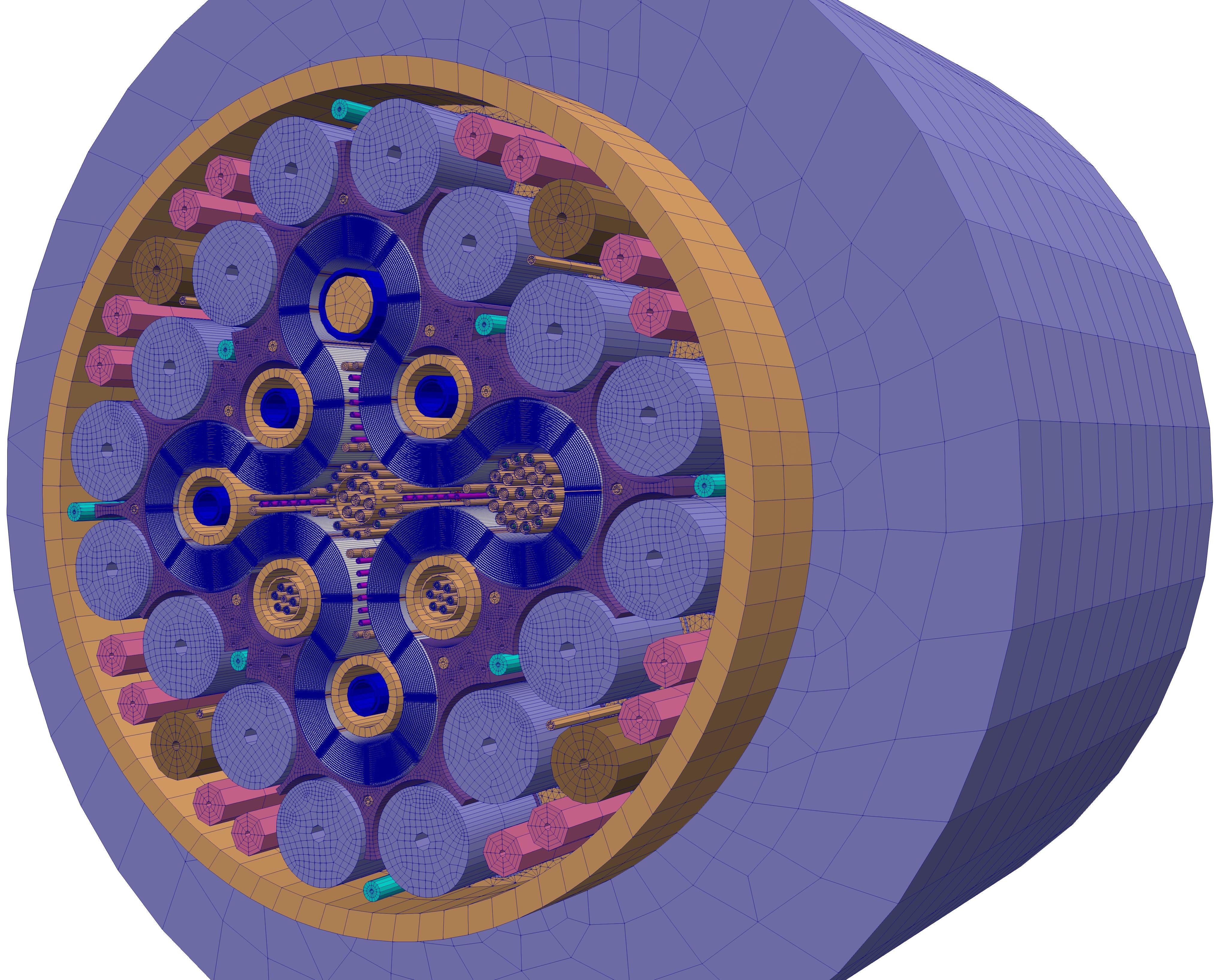
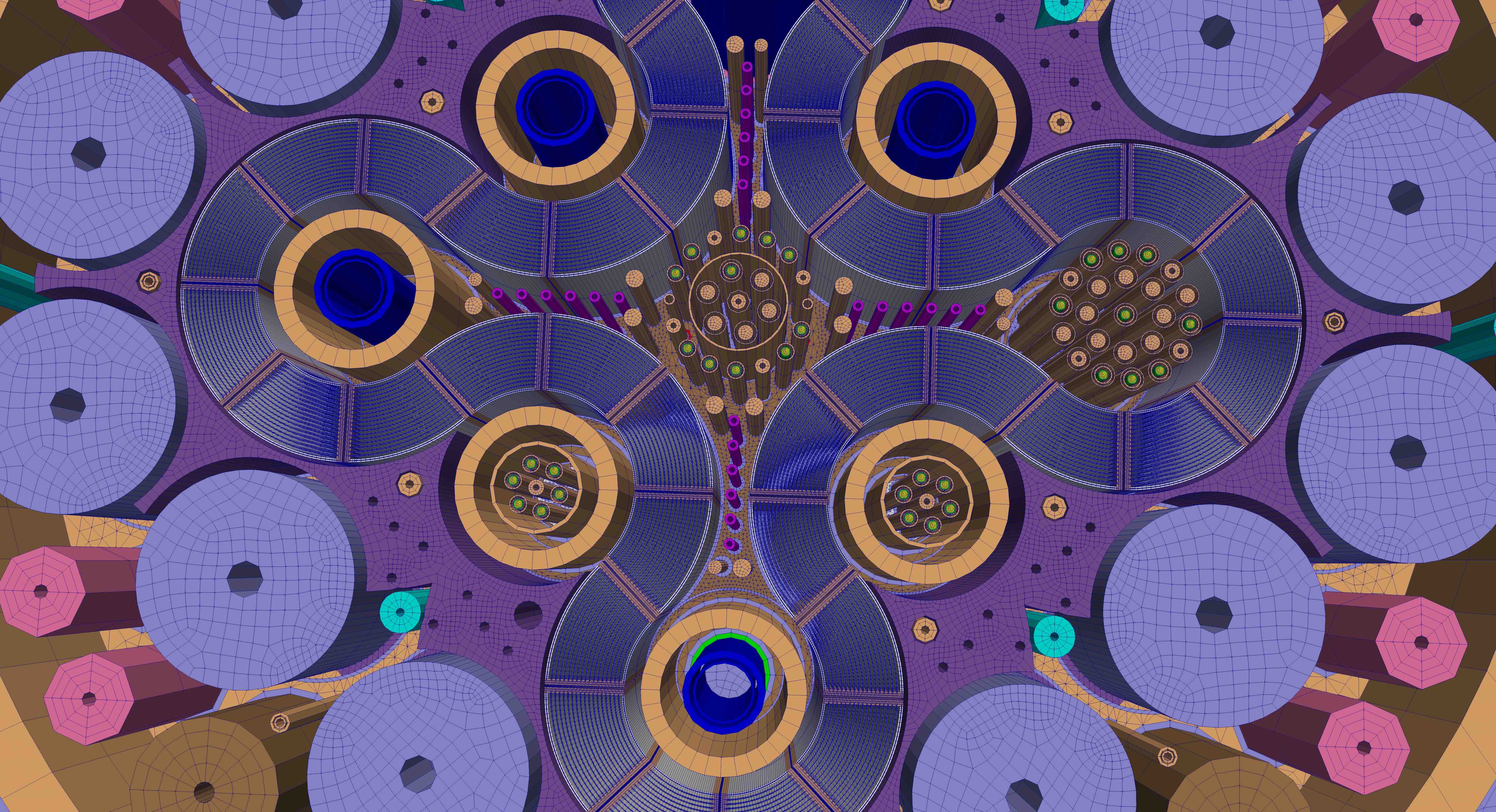
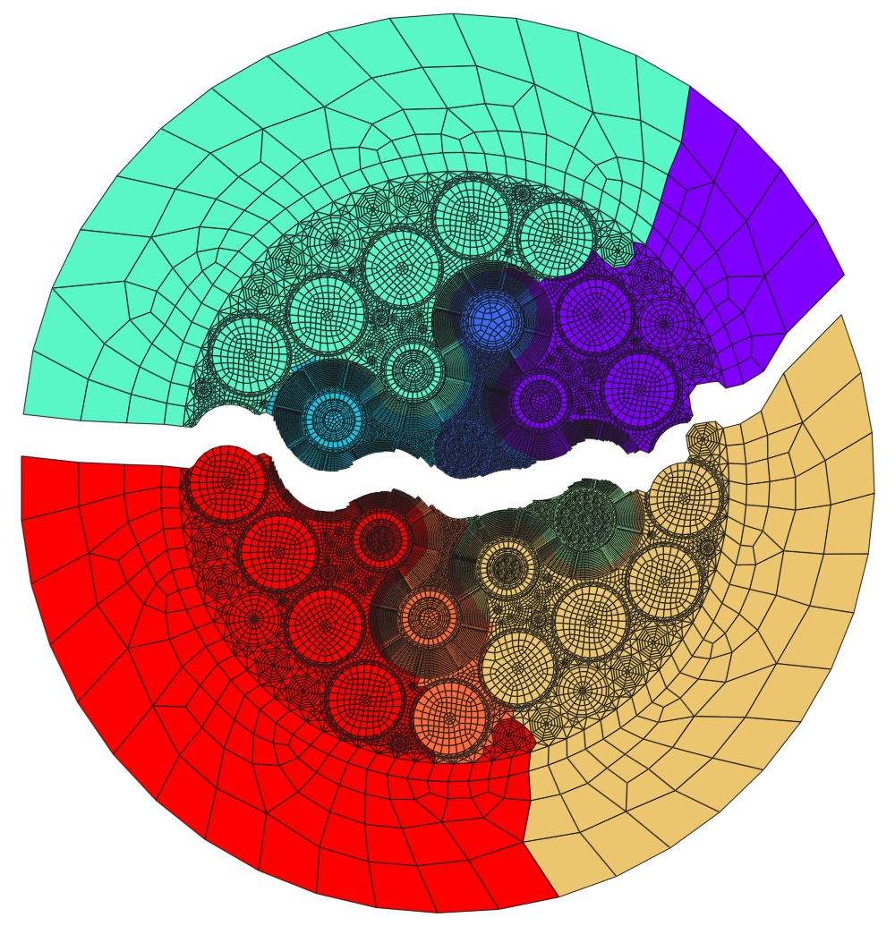
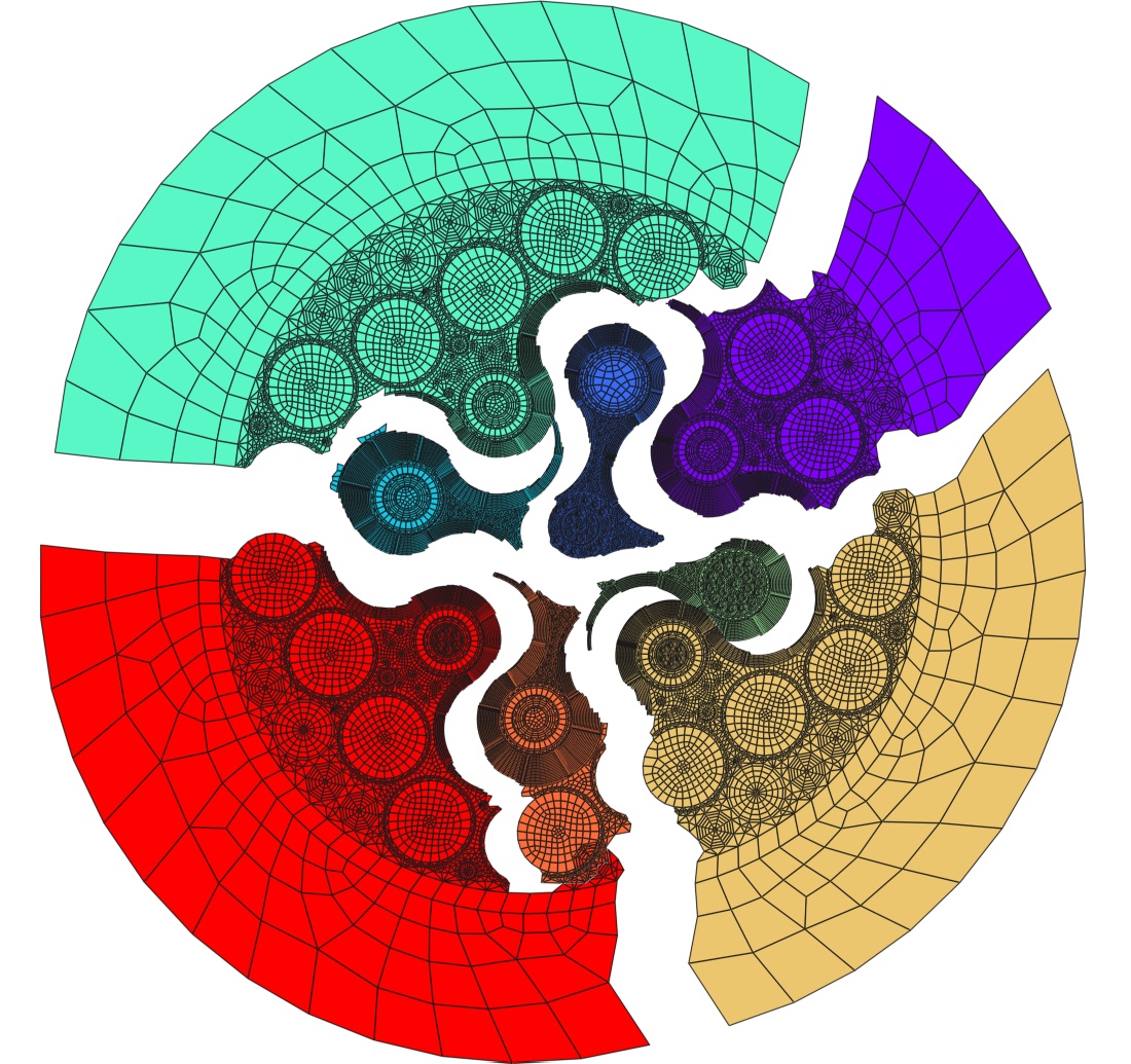
Figure 1: 3D unstructured mesh. Right: zoom-in picture of the top mesh. Different colors correspond to different materials. 


For convenience, let us define some operators:




$${\mathbbl{\mathbb{L}}}\mathbf{\Psi}\equiv\begin{bmatrix}\displaystyle{\mathbbl{{L}}}_{1}\Psi_{1},\displaystyle{\mathbbl{{L}}}_{2}\Psi_{2},\displaystyle\cdots,\displaystyle{\mathbbl{{L}}}_{G}\Psi_{G}\end{bmatrix}^{T},~{}{\mathbbl{{L}}}_{g}\Psi_{g}\equiv\vec{\nabla}\cdot\vec{\Omega}\Psi_{g}+\Sigma_{\mathrm{t},g}\Psi_{g},$$







$${\mathbbl{\mathbb{S}}}\mathbf{\Psi}\equiv\begin{bmatrix}\displaystyle{\mathbbl{{S}}}_{1}{\Psi_{1}},\displaystyle{\mathbbl{{S}}}_{2}{\Psi_{2}},\displaystyle\cdots,\displaystyle{\mathbbl{{S}}}_{G}{\Psi_{G}}\end{bmatrix}^{T},~{}{\mathbbl{{S}}}_{g}{\Psi_{g}}\equiv\sum_{g^{\prime}=1}^{G}\int_{\mathcal{S}}\Sigma_{\mathrm{s},g^{\prime}\rightarrow g}f_{g^{\prime}\rightarrow g}\Psi_{g^{\prime}}\,d\Omega^{\prime},$$







$${\mathbbl{\mathbb{F}}}\mathbf{\Psi}\equiv\begin{bmatrix}\displaystyle{\mathbbl{{F}}}_{1}\Psi_{1},\displaystyle{\mathbbl{{F}}}_{2}\Psi_{2},\cdots,\displaystyle{\mathbbl{{F}}}_{G}\Psi_{G}\end{bmatrix}^{T},~{}{\mathbbl{{F}}}_{g}\Psi_{g}\equiv\frac{1}{4\pi}\chi_{g}\sum_{g^{\prime}=1}^{G}\nu\Sigma_{\mathrm{f},g^{\prime}}\Phi_{g^{\prime}}.$$



Here ${\mathbbl{\mathbb{L}}}$ is the streaming-collision operator, ${\mathbbl{\mathbb{S}}}$ is the scattering operator and ${\mathbbl{\mathbb{F}}}$ is the fission operator.
Similarly, the operator for the boundary condition mapping from $\partial\mathcal{D}\times\mathcal{S}^{+}_{\vec{n}_{\mathrm{b}}}$ to $\partial\mathcal{D}\times\mathcal{S}^{-}_{\vec{n}_{\mathrm{b}}}$ is defined as




$${\mathbbl{\mathbb{B}}}\mathbf{\Psi}\equiv\begin{bmatrix}\displaystyle{\mathbbl{{B}}}_{1}\Psi_{1},\displaystyle{\mathbbl{{B}}}_{2}\Psi_{2},\displaystyle\cdots,\displaystyle{\mathbbl{{B}}}_{G}\Psi_{G}\\
\end{bmatrix}^{T},~{}{\mathbbl{{B}}}_{g}\Psi_{g}\equiv\alpha^{\text{s}}_{g}\Psi_{g}(\vec{\Omega}_{r})+\alpha^{\text{d}}_{g}\frac{\int_{\vec{\Omega}^{\prime}\cdot\vec{n}_{\mathrm{b}}>0}\left|\vec{\Omega}^{\prime}\cdot\vec{n}_{\mathrm{b}}\right|\Psi_{g}(\vec{\Omega}^{\prime})\,d\Omega^{\prime}}{\int_{\vec{\Omega}^{\prime}\cdot\vec{n}_{\mathrm{b}}>0}\left|\vec{\Omega}^{\prime}\cdot\vec{n}_{\mathrm{b}}\right|\,d\Omega^{\prime}}.$$



where $\mathcal{S}^{\pm}_{\vec{n}_{\mathrm{b}}}=\left\{\vec{\Omega}\in\mathcal{S},\vec{\Omega}\cdot\vec{n}_{\mathrm{b}}\gtrless 0\right\}$ is a half angular space defined with respect to the unit vector $\vec{n}_{\mathrm{b}}$. Finally,
Eq. 1a is rewritten as



(2)

$${\mathbbl{\mathbb{L}}}\mathbf{\Psi}={\mathbbl{\mathbb{S}}}\mathbf{\Psi}+\frac{1}{k}{\mathbbl{\mathbb{F}}}\mathbf{\Psi},$$



with the boundary condition $\mathbf{\Psi}={\mathbbl{\mathbb{B}}}\mathbf{\Psi}$ corresponding to Eq. 1b.




2.2 Spatial and angular discretizations


Before the weak form of  Eq. 2 is presented, some notations are introduced. An inner product is defined as




$$\left(\mathbf{a},\mathbf{b}\right)_{\mathcal{D}\times\mathcal{S}}\equiv\sum_{g=1}^{G}\int_{\mathcal{S}}\,d\Omega\int_{\mathcal{D}}\,dx\,a_{g}(\vec{x},\vec{\Omega})b_{g}(\vec{x},\vec{\Omega}),$$



where $\mathbf{a}$ and $\mathbf{b}$ are generic multigroup functions defined in $\mathcal{D}\times\mathcal{S}$.
We drop the subscript $\mathcal{D}\times\mathcal{S}$ for notation simplicity.
We also have a similar definition for the boundary integral as :




$$\left\langle\mathbf{a},\mathbf{b}\right\rangle\equiv\left\langle\mathbf{a},\mathbf{b}\right\rangle^{+}+\left\langle\mathbf{a},\mathbf{b}\right\rangle^{-},~{}\left\langle\mathbf{a},\mathbf{b}\right\rangle^{\pm}\equiv\sum_{g=1}^{G}\oint_{{\partial\mathcal{D}}}\,dx\int_{\mathcal{S}^{\pm}_{\vec{n}_{\mathrm{b}}}}\,d\Omega\,\left|\vec{\Omega}\cdot\vec{n}_{\mathrm{b}}\right|a_{g}(\vec{x},\vec{\Omega})b_{g}(\vec{x},\vec{\Omega}).\\$$



Following a standard finite element technique, we multiply a test function $\mathbf{\Psi}^{\ast}$ with Eq. 2, and then integrate over the phase space, $\mathcal{D}\times\mathcal{S}$,



(3)

$$\left(\mathbf{\Psi}^{\ast},{\mathbbl{\mathbb{L}}}\mathbf{\Psi}\right)=\left(\mathbf{\Psi}^{\ast},{\mathbbl{\mathbb{S}}}\mathbf{\Psi}\right)+\frac{1}{k}\left(\mathbf{\Psi}^{\ast},{\mathbbl{\mathbb{F}}}\mathbf{\Psi}\right).$$



After some manipulations, the weak form reads as




(4)

$$\left({\mathbbl{\mathbb{L}}}^{\ast}\mathbf{\Psi}^{\ast},\mathbf{\Psi}\right)+\left\langle\mathbf{\Psi}^{\ast},\mathbf{\Psi}\right\rangle^{+}-\left\langle\mathbf{\Psi}^{\ast},{\mathbbl{\mathbb{B}}}\mathbf{\Psi}\right\rangle^{-}=\left(\mathbf{\Psi}^{\ast},{\mathbbl{\mathbb{S}}}\mathbf{\Psi}\right)+\frac{1}{k}\left(\mathbf{\Psi}^{\ast},{\mathbbl{\mathbb{F}}}\mathbf{\Psi}\right),$$



where ${\mathbbl{\mathbb{L}}}^{\ast}$ is the adjoint operator of ${\mathbbl{\mathbb{L}}}$.
The form Eq. 4 is usually unstable, and here a stabilizing technique, SAAF (self-adjoint angular flux), is included to remedy this issue. In the SAAF method, the streaming-collision operator ${\mathbbl{\mathbb{L}}}$ is split into two parts (the streaming operator ${\mathbbl{\mathbb{L}}}_{1}$ and the collision operator ${\mathbbl{\mathbb{L}}}_{2}$),



(5)

$${\mathbbl{\mathbb{L}}}\mathbf{\Psi}\equiv{\mathbbl{\mathbb{L}}}_{1}\mathbf{\Psi}+{\mathbbl{\mathbb{L}}}_{2}\mathbf{\Psi},$$



where




$${\mathbbl{\mathbb{L}}}_{1}\mathbf{\Psi}\equiv\begin{bmatrix}{\mathbbl{{L}}}_{1,1}\Psi_{1},{\mathbbl{{L}}}_{1,2}\Psi_{2},\cdots,{\mathbbl{{L}}}_{1,G}\Psi_{G}\end{bmatrix}^{T},~{}{\mathbbl{{L}}}_{1,g}\Psi_{g}\equiv\vec{\Omega}\cdot\vec{\nabla}\Psi_{g},$$







$${\mathbbl{\mathbb{L}}}_{2}\mathbf{\Psi}\equiv\begin{bmatrix}{\mathbbl{{L}}}_{2,1}\Psi_{1},{\mathbbl{{L}}}_{2,2}\Psi_{2},\cdots,{\mathbbl{{L}}}_{2,G}\Psi_{G}\end{bmatrix}^{T},~{}{\mathbbl{{L}}}_{2,g}\Psi_{g}\equiv{\Sigma_{\mathrm{t},g}}{\Psi_{g}}.$$



The “inverse” of ${\mathbbl{\mathbb{L}}}_{2}$ is further defined as




$${\mathbbl{\mathbb{L}}}^{-1}_{2}\mathbf{\Psi}\equiv\begin{bmatrix}{\mathbbl{{L}}}_{2,1}^{-1}\Psi_{1},{\mathbbl{{L}}}_{2,2}^{-1}\Psi_{2},\cdots,{\mathbbl{{L}}}_{2,G}^{-1}\Psi_{G}\end{bmatrix}^{T},~{}{\mathbbl{{L}}}_{2,g}^{-1}\Psi_{g}={\Psi_{g}}/{\Sigma_{\mathrm{t},g}}.$$



It is easy to verify that ${\mathbbl{\mathbb{L}}}^{-1}_{2}{\mathbbl{\mathbb{L}}}_{2}={\mathbbl{\mathbb{I}}}$, ${\mathbbl{\mathbb{L}}}^{\ast}_{2}={\mathbbl{\mathbb{L}}}_{2}$, ${\mathbbl{\mathbb{L}}}^{\ast}_{1}=-{\mathbbl{\mathbb{L}}}_{1}$ and ${\mathbbl{\mathbb{L}}}_{1}{\mathbbl{\mathbb{L}}}_{2}={\mathbbl{\mathbb{L}}}_{2}{\mathbbl{\mathbb{L}}}_{1}$. With rearranging  Eq. 2, we have



(6)

$$\mathbf{\Psi}={\mathbbl{\mathbb{L}}}^{-1}_{2}\left(\frac{1}{k}{\mathbbl{\mathbb{F}}}\mathbf{\Psi}+{\mathbbl{\mathbb{S}}}\mathbf{\Psi}-{\mathbbl{\mathbb{L}}}_{1}\mathbf{\Psi}\right),$$



which is called the angular flux equation (AFE).
We substitute Eq. 6 into the streaming kernel of Eq. 4,




$$\boxed{\left({\mathbbl{\mathbb{L}}}_{1}^{\ast}\mathbf{\Psi}^{\ast},\mathbf{\Psi}\right)}+\left({\mathbbl{\mathbb{L}}}_{2}^{\ast}\mathbf{\Psi}^{\ast},\mathbf{\Psi}\right)+\left\langle\mathbf{\Psi}^{\ast},\mathbf{\Psi}\right\rangle^{+}-\left\langle\mathbf{\Psi}^{\ast},{\mathbbl{\mathbb{B}}}\mathbf{\Psi}\right\rangle^{-}=\left(\mathbf{\Psi}^{\ast},{\mathbbl{\mathbb{S}}}\mathbf{\Psi}\right)+\frac{1}{k}\left(\mathbf{\Psi}^{\ast},{\mathbbl{\mathbb{F}}}\mathbf{\Psi}\right),$$



and obtain the following form after a few manipulations




$$\boxed{\left({\mathbbl{\mathbb{L}}}_{1}\mathbf{\Psi}^{\ast},{\mathbbl{\mathbb{L}}}^{-1}_{2}{\mathbbl{\mathbb{L}}}_{1}\mathbf{\Psi}\right)+\left({\mathbbl{\mathbb{L}}}_{2}^{\ast}\mathbf{\Psi}^{\ast},\mathbf{\Psi}\right)+\left\langle\mathbf{\Psi}^{\ast},\mathbf{\Psi}\right\rangle^{+}}-\left\langle\mathbf{\Psi}^{\ast},{\mathbbl{\mathbb{B}}}\mathbf{\Psi}\right\rangle^{-}$$




$$=\left({\mathbbl{\mathbb{L}}}^{-1}_{2}{\mathbbl{\mathbb{L}}}\mathbf{\Psi}^{\ast},{\mathbbl{\mathbb{S}}}\mathbf{\Psi}\right)+\frac{1}{k}\left({\mathbbl{\mathbb{L}}}^{-1}_{2}{\mathbbl{\mathbb{L}}}\mathbf{\Psi}^{\ast},{\mathbbl{\mathbb{F}}}\mathbf{\Psi}\right).$$



We noticed that the boxed kernels are symmetric positive definite (SPD), and the calculation of the SPD system is possible using the multilevel method equipped with algebraic coarse spaces.
SAAF is equivalent to SUPG (Streamline upwind/Petrov-Galerkin) [3] with the inverse of group-wise total cross sections as the stabilization parameter. Finally, we denote the weak form obtained using the SAAF method as



(7)

$$\mathbbm{a}\left(\mathbf{\Psi}^{\ast},\mathbf{\Psi}\right)=\frac{1}{k}\mathbbm{f}\left(\mathbf{\Psi}^{\ast},\mathbf{\Psi}\right),$$



with




$$\mathbbm{a}\left(\mathbf{\Psi}^{\ast},\mathbf{\Psi}\right)\equiv
\left({\mathbbl{\mathbb{L}}}_{1}\mathbf{\Psi}^{\ast},{\mathbbl{\mathbb{L}}}^{-1}_{2}{\mathbbl{\mathbb{L}}}_{1}\mathbf{\Psi}\right)+\left({\mathbbl{\mathbb{L}}}_{2}\mathbf{\Psi}^{\ast},\mathbf{\Psi}\right)+\left\langle\mathbf{\Psi}^{\ast},\mathbf{\Psi}\right\rangle^{+}$$






$$-\left({\mathbbl{\mathbb{L}}}^{-1}_{2}{\mathbbl{\mathbb{L}}}\mathbf{\Psi}^{\ast},{\mathbbl{\mathbb{S}}}\mathbf{\Psi}\right)-\left\langle\mathbf{\Psi}^{\ast},{\mathbbl{\mathbb{B}}}\mathbf{\Psi}\right\rangle^{-},$$




$$\mathbbm{f}\left(\mathbf{\Psi}^{\ast},\mathbf{\Psi}\right)\equiv
\left({\mathbbl{\mathbb{L}}}^{-1}_{2}{\mathbbl{\mathbb{L}}}\mathbf{\Psi}^{\ast},{\mathbbl{\mathbb{F}}}\mathbf{\Psi}\right).$$






The $S_{N}$ (discrete ordinates) method that can be thought of as a collocation method is considered for the angular discretization. Given an angular quadrature set $\left\{\vec{\Omega}_{d},w_{d},d=1,\cdots,{N_{d}}\right\}$ consisting of ${N_{d}}$ directions $\vec{\Omega}_{d}$ and weights $w_{d}$, the multigroup transport equations is solved along these directions and all angular integrations in the kernels are numerically evaluated with the angular quadrature. With the $S_{N}$ method, an integral of general functions over $\mathcal{S}$ is represented as a weighted summation, that is,




$$\int_{\mathcal{S}}\Psi_{g}\,d\Omega^{\prime}=\sum_{d=1}^{N_{d}}w_{d}\Psi_{g,d}.$$



It is straightforward to apply the technique to Eq. 7. Take the collision term as an example, we have



(8)

$$\left({\mathbbl{\mathbb{L}}}_{2}\mathbf{\Psi}^{\ast},\mathbf{\Psi}\right)=\displaystyle\sum_{g=1}^{G}\int_{\mathcal{S}}\,d\Omega\left(\Sigma_{\mathrm{t},g}\Psi_{g}^{\ast},\Psi_{g}\right)_{\mathcal{D}}=\displaystyle\sum_{g=1}^{G}\sum_{d=1}^{N_{d}}w_{d}\left(\Sigma_{\mathrm{t},g}\Psi_{g,d}^{\ast},\Psi_{g,d}\right)_{\mathcal{D}},$$



where $(\cdot,\cdot)_{\mathcal{D}}$ denotes that the integral is taken over $\mathcal{D}$ only. For the spatial discretization, the first-order Lagrange finite element is applied to $(\cdot,\cdot)_{\mathcal{D}}$. For more details on the angular and spatial discretization of the neutron transport equations used in this work, please see [33].
After the angular and spatial discretization, a large eigenvalue system with the dense coupling block matrices in the energy and angle is produced. The potential
dense matrix in energy is generated because a high energy neutron can be scattered down to a low energy group (down-scattering) and a low energy neutron can be also scattered up
to a high energy group (up-scattering). The equation is fully coupled in the angle. We will introduce a scalable eigenvalue solver in next Section to
handle the large system of eigenvalue equations.



3 Scalable parallel algorithm framework


In this Section, we describe the parallel algorithm framework consisting of the Newton method for calculating the nonlinear system of equations, the Krylov subspace method for solving the Jacobian system and the Schwarz preconditioner for accelerating the linear solver.


The corresponding agebraic system of equations for Eq. 7 reads as



(9)

$$\mathcal{A}\mathbf{\Psi}=\frac{1}{k}\mathcal{B}\mathbf{\Psi},$$



where $\mathbf{\Psi}$ is also used to represent the solution vector that corresponds to the nodal values of the neutron flux at the mesh vertices, $\mathcal{A}$ is the corresponding matrix of
$\mathbbm{a}$, and $\mathcal{B}$ is the corresponding matrix of $\mathbbm{f}$. Note that the matrices $\mathcal{A}$ and $\mathcal{B}$ are not necessary to be formed
explicitly, and we will have a detailed discussion on this shortly. The simplest algorithm for the eigenvalue calculation of Eq. 9 is the inverse power iteration, shown
in Alg. 1, that works well only when the ratio of the minimum eigenvalue to the second smallest eigenvalue is sufficient small, but it converges slow or even fails to converge when the ratio is close to “1”.


Algorithm 1  Inverse power iteration. “$\leftarrow$” represents that the corresponding vector is scaled in place. $\max_{e}$ is the maximum number of inverse power iterations. $\text{tol}_{\mathbf{\Psi}}$ and $\text{tol}_{k}$ are relative tolerances for the eigenvalue and the eigenvector, respectively. 


1:Initialize $\mathbf{\Psi}_{0}$



2:Compute eigenvalue: $k_{0}=\lVert\mathcal{B}\mathbf{\Psi}_{0}\rVert$



3:Scale $\displaystyle\mathcal{B}\mathbf{\Psi}_{0}\leftarrow\frac{1}{k_{0}}\mathcal{B}\mathbf{\Psi}_{0}$



4:for $n=0,...,\max_{e}$ do



5:     $\mathcal{A}\mathbf{\Psi}_{n+1}=\mathcal{B}\mathbf{\Psi}_{n}$



6:     $k_{n+1}=\lVert\mathcal{B}\mathbf{\Psi}_{n+1}\rVert$



7:     Scale $\displaystyle\mathcal{B}\mathbf{\Psi}_{n+1}\leftarrow\frac{1}{k_{n+1}}\mathcal{B}\mathbf{\Psi}_{n+1}$



8:     if $\frac{\lVert\mathbf{\Psi}_{n+1}-\mathbf{\Psi}_{n}\rVert}{\lVert\mathbf{\Psi}_{n}\rVert}<\text{tol}_{\mathbf{\Psi}}$ and $\frac{|k_{n+1}-k_{n}|}{|k_{n}|}<\text{tol}_{k}$  then



9:         Break



10:     end if


11:end for


12:Output $k_{n+1}$ and $\mathbf{\Psi}_{n+1}$





The difficulty is overcome by a Newton method that accelerates the convergence. To take the advantage of Newton,
lines 5 and 6 of Alg. 1 are rewritten as follows:



(10)

$$\mathcal{F}(\mathbf{\Psi})=\begin{array}[]{llll}\displaystyle\mathcal{A}\mathbf{\Psi}-\frac{1}{\lVert\mathcal{B}\mathbf{\Psi}\rVert}\mathcal{B}\mathbf{\Psi}.\\
\end{array}$$



And then an inexact Newton is applied to Eq. 10. More precisely, for a given $\mathbf{\Psi}_{n}$, the new solution is updated as follows:



(11)

$$\mathbf{\Psi}_{n+1}=\mathbf{\Psi}_{n}+\bar{\mathbf{\Psi}}_{n}.$$



Here $\bar{\mathbf{\Psi}}_{n}$ is the Newton update direction obtained by solving the following Jacobian system of equations



(12)

$$\mathcal{J}(\mathbf{\Psi}_{n})\bar{\mathbf{\Psi}}_{n}=-\mathcal{F}(\mathbf{\Psi}_{n}),$$



where $\mathcal{J}(\mathbf{\Psi}_{n})$ is the Jacobian matrix at $\mathbf{\Psi}_{n}$, and $\mathcal{F}(\mathbf{\Psi}_{n})$ is the nonlinear function residual evaluated at $\mathbf{\Psi}_{n}$. To save the memory, $\mathcal{J}(\mathbf{\Psi}_{n})$
is not excplitly formed, instead, it is carried out in a matrix-free manner. The corresponding Newton is referred to as “Jacobian-free Newton” method [11]. That is, a matrix-vector product, $\mathcal{J}(\mathbf{\Psi}_{n})\bar{\mathbf{\Psi}}_{n}$, is approximated by




$$\mathcal{J}(\mathbf{\Psi}_{n})\bar{\mathbf{\Psi}}_{n}=\frac{\mathcal{F}(\mathbf{\Psi}_{n}+\delta\bar{\mathbf{\Psi}}_{n})-\mathcal{F}(\mathbf{\Psi}_{n})}{\delta},$$



where $\delta$ is a small permutation that is a square root of the machine epsilon in this paper. Eq. 12
is solved using an iterative method such as GMRES [24], and a preconditioner is required to construct a scalable and efficient parallel solver. Let us rewrite Eq. 12
as a preconditioned form



(13)

$$\mathcal{J}\mathcal{P}^{-1}\mathcal{P}\bar{\mathbf{\Psi}}=-\mathcal{F},$$



where $\mathcal{P}$ is the preconditioning matrix that is often an approximation to $\mathcal{J}$, and $\mathcal{P}^{-1}$ is a preconditioning process. The Jacobian $\mathcal{J}$ is carried out in a matrix-free manner since it has dense diagonal blocks since all groups and all directions are coupled through the fission term and the scattering term. The preconditioning matrix $\mathcal{P}$ is formed explicitly by only taking into consideration the first three terms of Eq. 7 since they form a SPD matrix that can be calculated using the multilevel method with algebraic coarse spaces. In fact, the angular fluxes in the energy and angle are independent in the first three terms of Eq. 7. If the variables were ordered group-by-group and direction-by-direction, $\mathcal{P}$ is written as



(14)

$$\mathcal{P}=\left[\begin{array}[]{llllll}\mathcal{P}_{0,0}&&&\\
&\mathcal{P}_{1,1}&&\\
&&\ddots&\\
&&&\mathcal{P}_{G,G}\\
\end{array}\right],$$



where $P_{g,g}$ is a block diagonal matrix for the $g$th energy group expressed as



(15)

$$\mathcal{P}_{g,g}=\left[\begin{array}[]{llllll}\mathcal{P}^{(0,0)}_{g,g}&&&\\
&\mathcal{P}^{(1,1)}_{g,g}&&\\
&&\ddots&\\
&&&\mathcal{P}^{(N_{d},N_{d})}_{g,g}\\
\end{array}\right].$$



Here $G$ is the number of energy groups, and $N_{d}$ is the number of angular directions per energy group. $\mathcal{P}_{g,g^{\prime}}$ represents the coupling matrix between groups $g$ and $g^{\prime}$. If the scattering and the fission
terms were taken into account, $\mathcal{P}$ would be a fully coupled matrix instead of the diagonal matrix shown in Eq. 14, that is, $\mathcal{P}_{g,g^{\prime}}\neq 0\text{~{}when~{}}g\neq g^{\prime}$.
$\mathcal{P}_{g,g}^{(d,d^{\prime})}$ represents the coupling matrix between angular directions $d$ and $d^{\prime}$ in the $g$th group. Similarly, if the fission term and the scattering term were considered in the preconditioning matrix,
$\mathcal{P}^{(d,d^{\prime})}_{g,g}$ would be a fully coupled dense matrix, that is, $\mathcal{P}^{(d,d^{\prime})}_{g,g}\neq 0\text{~{}when~{}}d\neq d^{\prime}$. For the given group $g$ and direction $d$, $\mathcal{P}^{(d,d)}_{g,g}$ is a large sparse matrix
obtained from the spatial discretization. It is easy to note that the block structure in Eq. 14 corresponds to the multigroup approximation, and that in Eq. 15 corresponds to the angular discretization.


Generally speaking, a preconditioning procedure is designed to find the solution of the following residual equations,



(16)

$$\mathcal{P}e=r,$$



where $r$ is the residual vector from the outer solver (GMRES). To carry out the simulation in parallel, the mesh $\mathcal{D}_{h}$, corresponding to a triangulation of $\mathcal{D}$, is partitioned into $np$ ($np$ is the number of processor cores) submeshes $\mathcal{D}_{h,i},i=1,2,..,np$. This is accomplished by a hierarchical partitioning method since most
existing partitioners such as ParMETIS [9] do not work well when the number of processor cores is close to or more than 10,000. The basic idea of the hierarchical partitioning is to apply an existing partitioner such as ParMETIS or PT-Scotch [5] twice. The computational mesh $\mathcal{D}_{h}$ is first partitioned
into $np_{1}$ “big” submeshes ($np_{1}$ often is the number of compute nodes), and each “big” submesh is further divided into $np_{2}$ ($np_{2}$
is the number of processor cores per compute node) small submeshes. A 2D example with assuming that each compute node has $4$ processor cores is shown in Fig. 2, where the mesh is partitioned into $2$ “big” submeshes, and then
each “big” submesh is further divided into $4$ small submeshes, and finally we have $8$ small submeshes in total. Note that the hierarchical partitioning works for 3D meshes, and the 2D example is shown for the demonstration.






Figure 2: Hierarchical partitioning. A mesh is paritioned into $2$ “big” submeshes shown in the left, and then each “big” submesh is further into
$4$ small submeshes. We finally have 8 submeshes. 


Using the hierarchal partitioning method, we are able to not only produce a large number of submeshes, but also minimize the off-node communication since $np_{2}$ small submeshes on a compute node are physically connected and the communication between them is cheap. Interested readers are referred to our previous works [13, 18] for more details of the hierarchical partitioning. Let us denote the submatrix and the subvectors associated with a submesh $\mathcal{D}_{h,i}$ as $\mathcal{P}_{i}$, $e_{i}$ and $r_{i}$, respectively.
We define a restriction operator, $R_{i}$, that restricts a global vector $r$ to a nonoverlapping submesh, that is, $r_{i}$ = $R_{i}r$. With those notations, the one-level nonoverlapping Schwarz preconditioner is expressed as



(17)

$$\mathcal{P}^{-1}_{one}=\sum_{i=1}^{np}R_{i}^{T}\mathcal{P}_{i}^{-1}R_{i},~{}~{}\mathcal{P}_{i}=R_{i}\mathcal{P}R_{i}^{T}$$



where $\mathcal{P}_{i}^{-1}$ is a subdomain solver that is a successive over-relaxation (SOR) algorithm in this paper. The subdomain restriction $R_{i}$ does not extract any overlapping values. The overlapping version of Eq. 17 has been successfully employed in our previous works [13, 14, 16, 17] for elasticity equations, incompressible flows and fluid-structure interactions. Interested readers are referred to [27, 29] for more details on the Schwraz methods.
After many experiments, we find that the nonoverlapping Schwarz preconditioner is able to maintain a strong scalability for the targeting applications when it is equipped with the subspace-based coarse spaces to be introduced shortly, and meanwhile the nonoverlapping Schwarz preconditioner uses less memory and communication compared with the overlapping version since no ghosting matrix entries need to be stored and exchanged. Coarse spaces need to be investigated for $\mathcal{P}^{-1}_{one}$ to form its multilevel version when the number of processor cores is large, the materials are heterogeneous and the computational domain is complex. Let us denote $L$ spaces as $\mathcal{D}_{h}^{(1)},\mathcal{D}_{h}^{(2)},...,\mathcal{D}_{h}^{(L)}$, and the associated operators as $\mathcal{P}^{(1)},\mathcal{P}^{(2)},...,\mathcal{P}^{(L)}$. Here $\mathcal{D}_{h}^{(1)}=\mathcal{D}_{h}$ and $\mathcal{P}^{(1)}=\mathcal{P}$. The interpolation operator from $\mathcal{D}_{h}^{(l+1)}$ to $\mathcal{D}_{h}^{(l)}$ is denoted as $I_{l+1}^{l}$ , and the corresponding restriction operator from $\mathcal{D}^{(l)}_{h}$ to
$\mathcal{D}^{(l+1)}_{h}$ is $(I_{l+1}^{l})^{T}$. A multilevel additive Schwarz preconditioner (abbreviated as “MASM”) is summarized as Alg. 2.


Algorithm 2  MASM($\mathcal{P}^{(l)},e^{(l)},r^{(l)}$)


1:if $l=L$ then



2:     Solve $\mathcal{P}^{(L)}e^{(L)}=r^{(L)}$ with a redundant direct solver on each compute node



3:else


4:     Pre-solve $\mathcal{P}^{(l)}e^{(l)}=r^{(l)}$ using an iterative solver preconditioned by $(\mathcal{P}^{(l)}_{one})^{-1}$



5:     Set $\bar{r}^{(l)}=r^{(l)}-\mathcal{P}^{(l)}e^{(l)}$



6:     Apply the restriction: $\bar{r}^{(l+1)}=(I_{l+1}^{l})^{T}\bar{r}^{(l)}$



7:     $z^{(l+1)}$ = MASM($\mathcal{P}^{(l+1)},z^{(l+1)},\bar{r}^{(l+1)}$)



8:     Apply the interpolation: $z^{(l)}=I_{l+1}^{l}z^{(l+1)}$



9:     Correct the solution: $e^{(l)}=e^{(l)}+z^{(l)}$



10:     Post-solve $\mathcal{P}^{(l)}e^{(l)}=r^{(l)}$ using an iterative solver preconditioned by $(\mathcal{P}^{(l)}_{one})^{-1}$



11:end if


12:Return $e^{(l)}$





The fundamental motivation behind Alg. 2 is that the high frequency mode of the solution is efficiently resolved using an iterative method together with the preconditioner $\mathcal{P}^{-1}_{one}$, and then the remaining low high frequencies will be handled in the coarse levels. The performance of Alg. 2 is largely affected by how to construct coarse spaces and their associated interpolations. Generally speaking, there are
two ways to construct a set of coarse spaces. The first approach is to geometrically coarsen the fine mesh $\mathcal{D}_{h}$ to generate coarse meshes, which has been shown to be powerful
in our previous works [13] for elasticity problems and [12, 14, 15] for fluid-structure interactions. However, the geometry of the targeting application is complex so that it is nontrivial to setup a geometric mesh coarsening algorithm. The second one is to construct coarse spaces without querying any mesh information, instead, the coarse spaces and their interpolations are derived based on the matrix information only. The second approach has been successfully applied for different applications [7, 32, 34]. However, it is well known that the setup phase of the algebraic-version preconditioner is not strongly scalable in terms of the compute time since the matrix coarsening and the interpolation construction are expensive [34]. Fortunately, the overall algorithm can be still scalable if the preconditioner setup phase accounts for a reasonably small portion of the total compute time. We will introduce such a new subspace-based coarsening algorithm that
the preconditioner setup time is significantly reduced and the overall algorithm is able to maintain a good scalability with more than 10,000 processor cores. We
will give a detailed description of the proposed coarsening algorithm in next Section.



4 Coarse spaces


In this section, we discuss a coarse space construction for Alg. 2. First, a matrix coarsening algorithm based on subspace is introduced, where
the “grid” point selection is accomplished using a submatrix instead of the global matrix. A subinterpolation is constructed based on the splitting of the coarse points and the fine points, and the global interpolation is built from the subinterpolation.



4.1 Matrix coarsening based on subspace


According to Eq. 14 and Eq. 15, it is easily found that $\mathcal{P}$ is a block diagonal matrix and each block corresponds to the spatial discretization of Eq. 2 for a given energy group and angular direction. Furthermore, there is no coupling between a block and the other blocks since we ignore the scattering and the fission terms in the preconditioning matrix. The individual matrix blocks are similar to each other in the sense that they correspond to the same continuous operators and share the same computational mesh $\mathcal{D}_{h}$. The differences between them come from different materials (i.e. cross sections) being used by different energy groups. Our motivation here is to
coarsen a block of $\mathcal{P}$ instead of the entire matrix to generate subinterpolations, and then the subinterpolations are expanded to covered the entire space by defining an expanding
operator. The benefit of this approach is potentially save a lot of the setup time and also the memory usage since the coarsening phase operates on a much smaller data set. Let us define a restriction $R_{s,i}$ that extracts the corresponding components from the entire vector $r$ for a given angular direction and energy group to form a subspace vector $r_{s,i},i=1,2,...,G\times N_{d}$, that is,




$$r_{s,i}=R_{s,i}r\equiv\left(\begin{array}[]{lll}\mathbb{I}&0\end{array}\right)\left(\begin{array}[]{lll}r_{s,i}\\
r/r_{s,i}\end{array}\right),$$



where “$/$” denotes the components in $r$ but not in $r_{s,i}$. The choice of energy groups and angular directions is arbitrary in this paper, and we use the first energy group and angular direction, that is, $i=1$. Without any confusion, we drop the second subscript of $r_{s,1}$ and $R_{s,1}$, and denote them as $r_{s}$ and $R_{s}$, respectively, for the simplicity of notations. With these notations, a subspace preconditioning matrix (for the first energy group and angular direction) is formed as



(18)

$$\mathcal{P}_{s}=R_{s}\mathcal{P}R_{s}^{T}.$$



Here $\mathcal{P}_{s}$ can be coarsened using one of the existing matrix coarsening algorithms. We use a hybrid method of the Ruge-St$\ddot{u}$ben (RS) coarsening [28] and the Cleary-Luby-Jones-Plassman (CLJP)
coarsening method [32]. For completeness, we briefly describe these methods here, and interested readers are referred to [22, 23, 34] for more details. Before starting a coarsening process, a “strength” matrix (graph), $\mathcal{G}=(V,E)$, need to be constructed from $\mathcal{P}_{s}$ since
not all coefficients are equally important to determine the coarse spaces (grids) and we should consider the important coefficients only. Here $V$ is a set of all points in $\mathcal{P}_{s}$, that is, $V=\{v_{i}\}$, and the size of $V$ is the number of rows of $\mathcal{P}_{s}$. $E$ is a set of the corresponding edges, that is, $E=\{\tilde{e}_{ij}\}$. An edge $\tilde{e}_{ij}$ is formed when $v_{i}$ strongly depends on $v_{j}$ or $v_{j}$ strongly influences $v_{i}$ according to
the following formula



(19)

$$-p_{ij}\geq\theta\max_{k\neq i}(-p_{ik}),$$



where $p_{ij}$ is an entity of $\mathcal{P}_{s}$, and $\theta$ is the strength threshold that sometimes has an important impact on the overall algorithm performance because it changes the matrix complexities, the stencil sizes, and the solver convergence rate. A coarsening algorithm tries to split $V$ into either coarse points (C-point), denoted as $C$, which will be taken into the next level, or fine points (F-points), denoted as $F$, which will be interpolated by C-points.


The RS coarsening algorithm (also referred to as “classical” coarsening in some literatures) has two targets:


 

For each point $v_{j}$ that strongly influences an F-point $v_{i}$, $v_{j}$ is either a $C$-point or it shares a common C-point $v_{k}$ with $v_{i}$



 

$C$ should be a maximal independent set



“A1” is designed to insure the quality of interpolation, while “A2” controls the size of the coarse
space and the complexity of the operator. In practice, it is hardly to satisfy both conditions at the same time. The RS coarsening tries to meet A1 while uses A2 as a guideline and it is carried out in two passes. In the first pass, each point $v_{i}$ is assigned by a measure $\,\mathrm{m}_{i}$ that equals the number of the points strongly influenced by $v_{i}$, and the point with the maximum measure is selected as
C-point, $v_{c}$. All the points strongly influenced by $v_{c}$ are chosen as new F-points, $\{v_{f}\}$. For each unmarked point that strongly influences any point in $\{v_{f}\}$, its measure is increased by the number of F-points it influences. This procedure is repeated until all points are chosen as either C-points or F-points. In the second pass, the algorithm checks every strong F-F connection if two F-points have a common C-point. If there is no a common C-point, and then one of the two F-points is chosen as a C-point. The approach is summarized in Alg. 3. It is easily seen that the RS algorithm is inherently sequential.


Algorithm 3  Subspace based RS coarsening


1:Input: $\mathcal{P}$ $\triangleright$ Submatrix extraction



2:Extract a submatrix: $\mathcal{P}_{s}=R_{s}\mathcal{P}R_{s}^{T}$



3:Construct a strength matrix of $\mathcal{P}_{s}$, $\mathcal{G}=(V,E)$, according to  Eq. 19



4:Compute measures $\{m_{i}\}$ for all points in $V=\{v_{i}\}$



5:Set $C=\emptyset$, $F=\emptyset$



6:while $V\neq\emptyset$ do $\triangleright$ Pass 1



7:     Find a point $v\in V$ that has the maximum measure



8:     $C=C+v$



9:     Find the neighbors of $v$ (denoted as $V_{n}\subset V$) that strongly depend on $v$



10:     $V=V-v$



11:     $F=F+V_{n}$



12:     for $v_{n}\in V_{n}$ do



13:         Find the neighbors of $v_{n}$ (denoted as $V_{nn}\subset V$ ) that strongly influence $v_{n}$



14:         for $v_{nn}\in V_{nn}$ do



15:              $m_{nn}$ = $m_{nn}+1$



16:         end for


17:     end for


18:     $V=V-V_{n}$



19:end while


20:for $v_{i}\in F$ do $\triangleright$ Pass 2



21:     Find the neighbors of $v_{i}$ (denoted as $F_{n}\subset F$) that strongly influence $v_{i}$



22:     for $v_{n}\in F_{n}$ do



23:         if $v_{n}$ and $v_{i}$ do not share a common C-point  then



24:              $F=F-v_{n}$



25:              $C=C+v_{n}$



26:         end if


27:     end for


28:end for


29:Output: $C$, $F$





A completely parallel coarsening approach is suggested in [6, 32]. It is based on a parallel maximal independent set (MIS)
algorithm as described in [22], and is often denoted as “CLJP” (Cleary-Luby-Jones-Plassman) in other literatures. The CLJP coarsening algorithm starts with adding a measure $m_{i}$ for each
point $v_{i}\in V$ just like the RS coarsening algorithm. Each $m_{i}$ is added by a small random value between $0$ and $1$ so that the points are distinctive even if the original
measures are the same. It is now possible to find a local maximum of all the point measures independently in parallel. A point $v_{i}$ with the local maximal measure is selected as a C-point, and the measures of the neighboring points strongly influenced by $v_{i}$ are decreased by 1. Furthermore, for all the points $\{v_{j}\}$ that strongly depend on $v_{i}$, remove their connections to $v_{i}$. Examine all the points $\{v_{k}\}$ that depend on $v_{j}\in\{v_{j}\}$ whether or not they also depend on $v_{i}$. If $v_{i}$ is a common C-point of $v_{k}$ and $v_{j}$, remove the connection from $v_{k}$ to $v_{j}$ and decrease the measure of $v_{j}$ by 1. If the measure of $v_{j}\in\{v_{j}\}$ is smaller than 1, it is chosen as a F-point. This procedure is repeated until all points are selected as either C-points or F-points. The algorithm is summarized in Alg. 4.


Algorithm 4  Subspace based CIJP coarsening


1:Input: $\mathcal{P}$ $\triangleright$ Submatrix extraction



2:Extract a submatrix: $\mathcal{P}_{s}=R_{s}\mathcal{P}R_{s}^{T}$



3:Construct a strength matrix of $\mathcal{P}_{s}$, $\mathcal{G}=(V,E)$, according to  Eq. 19



4:Compute measure $\{m_{i}\}$ for all point in $V=\{v_{i}\}$



5:Set $C=\emptyset$, and $F=\emptyset$



6:Add a random between 0 and 1 to each $m_{i}\in\{m_{i}\}$ $\triangleright$ Pass 1



7:while $V\neq\emptyset$ do



8:     Find a point $v\in V$ that has the local maximum measure



9:     $C=C+v$



10:     Find the neighbors of $v$ (denoted as $V_{n}\subset V$) that strongly depend on $v$



11:     for $v_{n}\in V_{n}$ do



12:         $m_{n}=m_{n}-1$



13:         Find the neighbors of $v_{n}$ (denoted as $V_{nn}\subset V$ ) that strongly depends on $v_{n}$



14:         for $v_{nn}\in V_{nn}$ do



15:              if $v_{nn}$ also depends on $v$ then



16:                  $m_{nn}=m_{nn}-1$



17:              end if


18:         end for


19:     end for


20:     for $v_{n}\in V_{n}$ do



21:         if $m_{n}<1$ then



22:              $F=F+v_{n}$



23:              $V=V-v_{n}$



24:         end if


25:     end for


26:     $V=V-v$



27:end while


28:Output: $C$, $F$





While this approach works well for many applications, another option that has been shown to be even better is the combination of the RS coarsening and the CIJP coarsening [32]. This coarsening starts with Alg. 3 of which the first pass is applied to the local graph independently in parallel. The interior C-points and F-points generated in Alg. 3 are used as an initial for Alg. 4. The resulting coarsening, which satisfies A1, fills the boundaries with further C-points and possibly adds a few in the interior of the subdomains. For convenience, the algorithm is denoted as “HCIJP” (hybrid CIJP coarsening, and it is also referred to as “Falgout” in [32]) and shown in Alg. 5.


Algorithm 5  Subspace based HCIJP coarsening


1:Input: $\mathcal{P}$ $\triangleright$ Submatrix extraction



2:Extract a submatrix: $\mathcal{P}_{s}=R_{s}\mathcal{P}R_{s}^{T}$



3:Construct a strength matrix of $\mathcal{P}_{s}$, $\mathcal{G}=(V,E)$, according to  Eq. 19



4:Compute measure $\{m_{i}\}$ for all point in $V=\{v_{i}\}$



5:Set $C=\emptyset$, and $F=\emptyset$



6:Apply the first pass of Alg. 3



7:Apply the first pass of Alg. 4



8:Output: $C$, $F$





While these approach work well for many applications, they sometimes lead
to high complexities. There are some options that can be used to resolve these issues. The first one is to loose A1 as: A F-point should strongly depends on at least one C-point. This approach often decreases the complexity, but the complexity can be still high and require more memory than desired. This is further improved by an aggressive coarsening algorithm that is most efficiently implemented by applying the coarsening algorithms twice,
The resulting aggressive coarsening algorithm is briefly described in
Alg. 6.


Algorithm 6  Subspace based aggressive HCIJP coarsening


1:Input: $\mathcal{P}$ $\triangleright$ Submatrix extraction



2:Extract a submatrix: $\mathcal{P}_{s}=R_{s}\mathcal{P}R_{s}^{T}$



3:Construct a strength matrix of $\mathcal{P}_{s}$, $\mathcal{G}=(V,E)$, according to  Eq. 19



4:Compute measure $\{m_{i}\}$ for all point in $V=\{v_{i}\}$



5:Set $C=\emptyset$, and $F=\emptyset$



6:Apply the first pass of Alg. 5 to $\mathcal{G}$



7:Apply the first pass of Alg. 5 to $C$



8:Output: $C$, $F$







4.2 Interpolation construction based on subspace


With a splitting $(C,F)$, we consider the construction of interpolation. For a given F-point $v_{i}$, its interpolation takes the form as follows:




$$e_{i}=\sum_{j\in C_{i}}w_{ij}e_{j},$$



where $C_{i}$ is the coarse interpolatory set of $v_{i}$, and $w_{ij}$ is an interpolation weight determing the contribution of $e_{j}$ to $e_{i}$. We
assume that an algebraically smooth error corresponds to a small residual, that is, $\mathcal{P}_{s}e\approx 0$ when $e$ is algebraically smooth. Let $V_{n,i}$ be the neighboring
points of $v_{i}$, which strongly or weakly influence $v_{i}$, and then the $i$th equation of $\mathcal{P}_{s}e\approx 0$ reads as



(20)

$$p_{ii}e_{i}+\sum_{j\in V_{n,i}}p_{ij}e_{j}\approx 0.$$



Here $V_{n,i}$ comprises three sets: $C_{i}$ (coarse neighbors), $F_{i}^{w}$ (weakly influencing neighbors) and $F_{i}^{s}$ (strongly influencing neighbors). A “classical”
interpolation, as described in [23], is constructed as



(21)

$$w_{ij}=-\frac{1}{p_{ii}+\sum_{k\in F^{w}_{i}p_{ik}}}(p_{ij}+\sum_{k\in F^{s}_{i}}\frac{p_{ik}p_{kj}}{\sum_{m\in C_{i}p_{km}}}).$$



Eq. Eq. 21 is easy to implement in parallel since it only involves immediate neighbors and only requires one layer of the ghosting points. This method is invalid if A1 is not met. Another interpolation scheme, often referred as “direction interpolation”, which only needs immediate neighbors and can be used when A1 is violated, is expressed as



(22)

$$w_{ij}=-\frac{p_{ij}}{p_{ii}}(\frac{\sum_{k\in V_{n,i}}p_{ik}}{\sum_{l\in C_{i}}p_{il}}).$$



If an aggressive coarsening scheme such as Alg. 6 is adopted, it is necessary to use a long range interpolation, such as a “multipass interpolation” as described in [28], in order to achieve a reasonable convergence. The “multipass” interpolation scheme starts with computing interpolating weights using Eq. 22 for the F-points immediately influenced by at least one C-point. In the second pass, for each F-point $v_{i}$ that have not been interpolated yet, find its neighboring interpolated F-points $v_{j}$ and then replace $e_{j}$ with $\sum_{k\in C_{j}}w_{jk}e_{k}$ in Eq. Eq. 20. A direct interpolation is then applied to the modified equation. We would like to refer interested readers to [7]
for more details on different interpolation approaches.
Let us denote the subinterpolation constructed using the submatrix $\mathcal{P}_{s}$ as $I_{s,2}^{1}$ from the second level to first level. And the full interpolation $I_{2}^{1}$ is expanded using the subinterpolation as follows



(23)

$$I_{2}^{1}=\sum_{i=1}^{G\times N_{d}}(R_{i}^{(1)})^{T}I_{s,2}^{1}R_{i}^{(2)}$$



where $R_{i}^{(l)}$ is the restriction operator defined on the $l$th level for the $i$th variable. The full coarse operator is computed using a Galerkin method



(24)

$$\mathcal{P}^{(2)}=(I_{2}^{1})^{T}\mathcal{P}^{(1)}I_{2}^{1}.$$



With the full coarse operator in Eq. 24 and the full interpolation in Eq. 23, the corresponding version of Alg. 2 is denoted
as “MASM${}_{\text{sub}}$”, while that equipped with the traditional coarse operators and interpolations is simply written as “MASM”. Note that the description in this Section focuses on generating one interpolation and one coarse operator, and it is straightforward to apply the idea to generate a sequence of coarse spaces.



5 Numerical results


In this section, we report the algorithm’s performance in terms of the compute time and the strong scalability for the eigenvalue calculation of the multigroup neutron transport equations for a realistic application, namely Advanced Test Reactor (ATR) that is located at the
Reactor Technology Complex of the Idaho National Laboratory (INL) and is a 250-MW high flux test reactor. The ATR core, as shown in Fig 1, contains 40 fuel elements arranging in a
serpentine annulus between and around nine flux traps. The algorithms are implemented based on PETSc [2] and hypre [20].
The numerical experiments are carried out on a supercomputer at INL, where each compute node has 36 processor cores (2.10 GHz per core) and the compute nodes are connected by a FDR InfiniBand Network of 56 Gbit/s. The problems are
solved with an inexact Newton Eq. 11 together with GMRES preconditioned by Alg. 2, where 4 iterations of the inverse power, as shown in Alg. 1, is used to generate an initial guess for Newton. In the Newton eigenvalue solver, a relative tolerance of $10^{-6}$
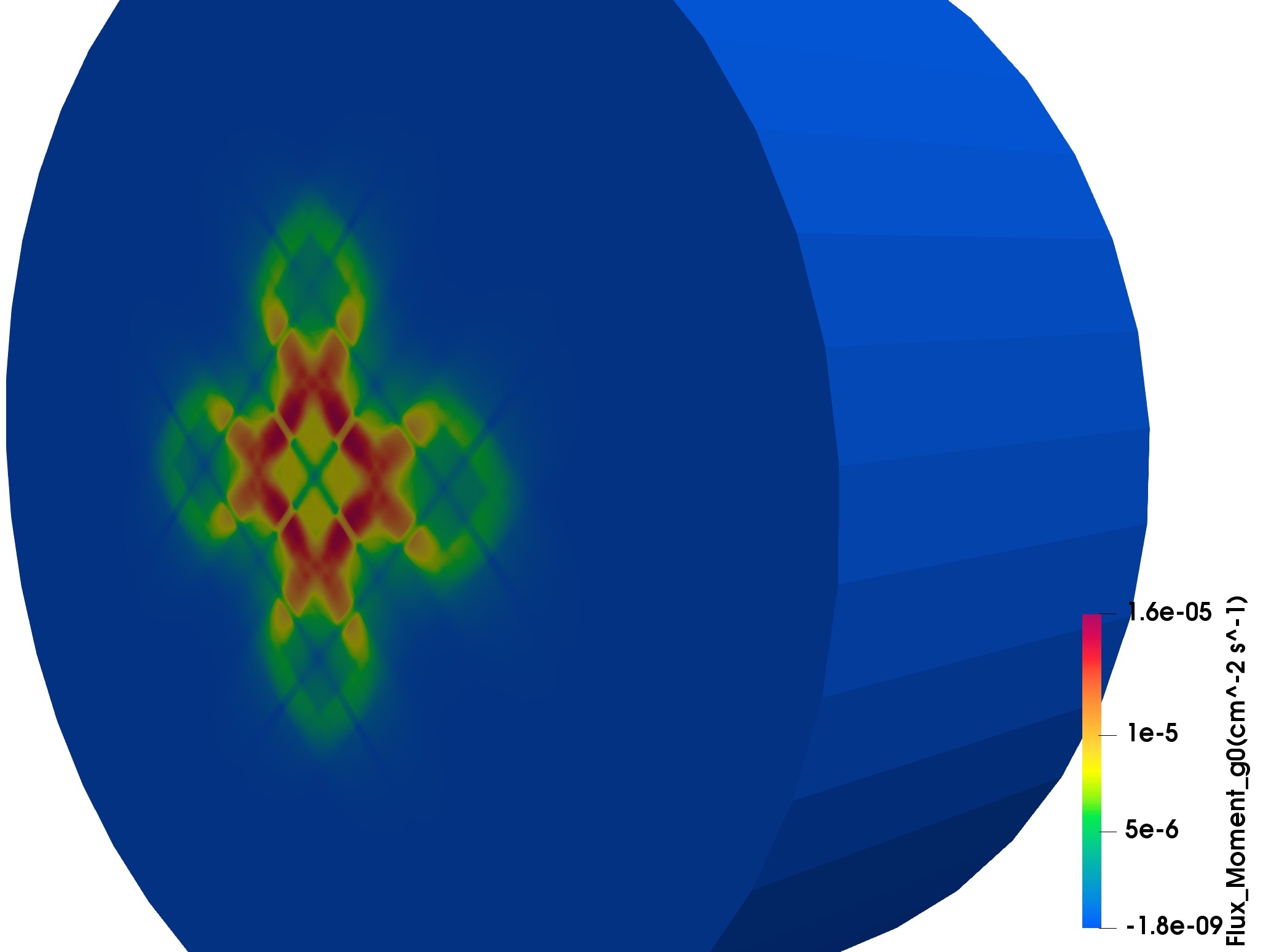
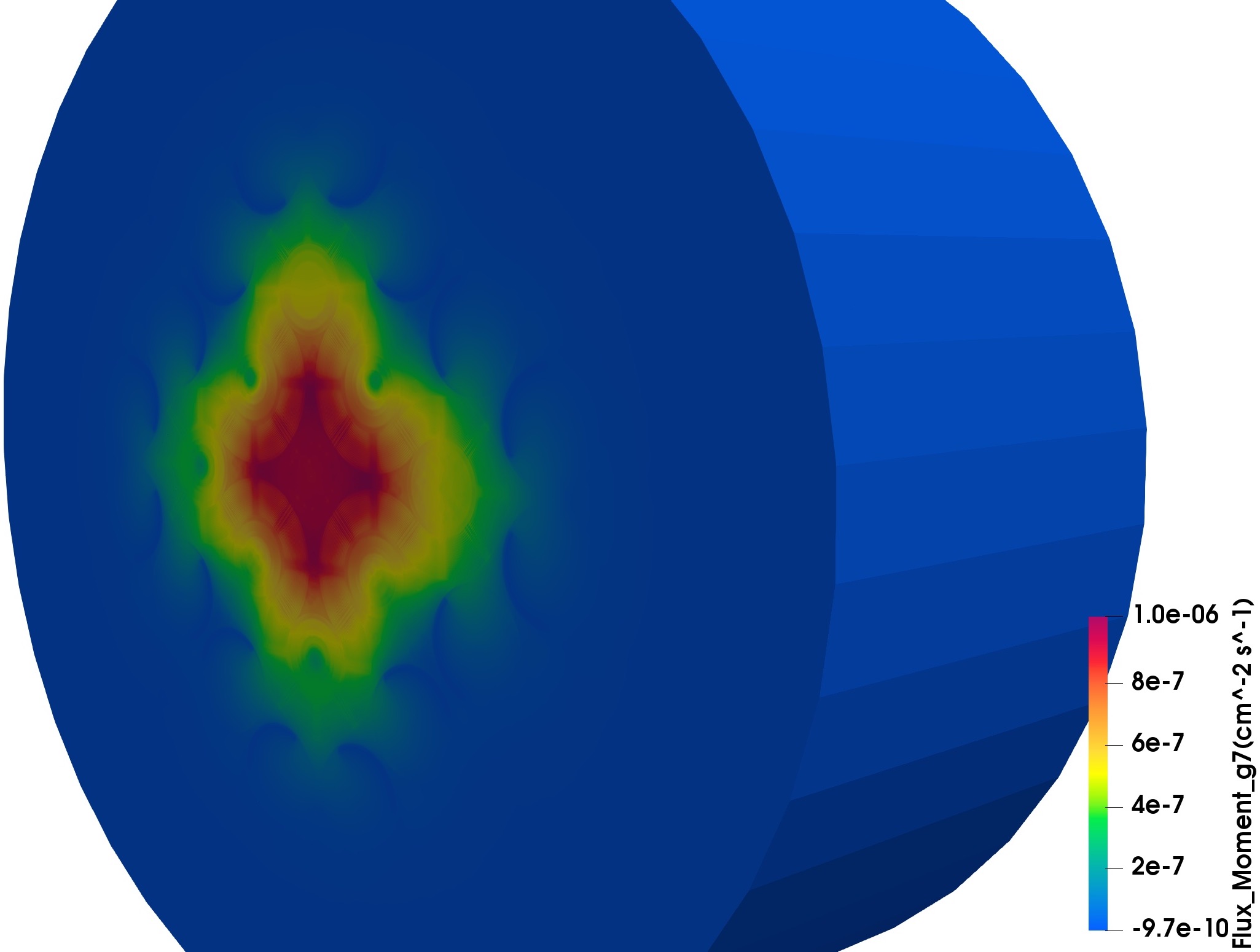
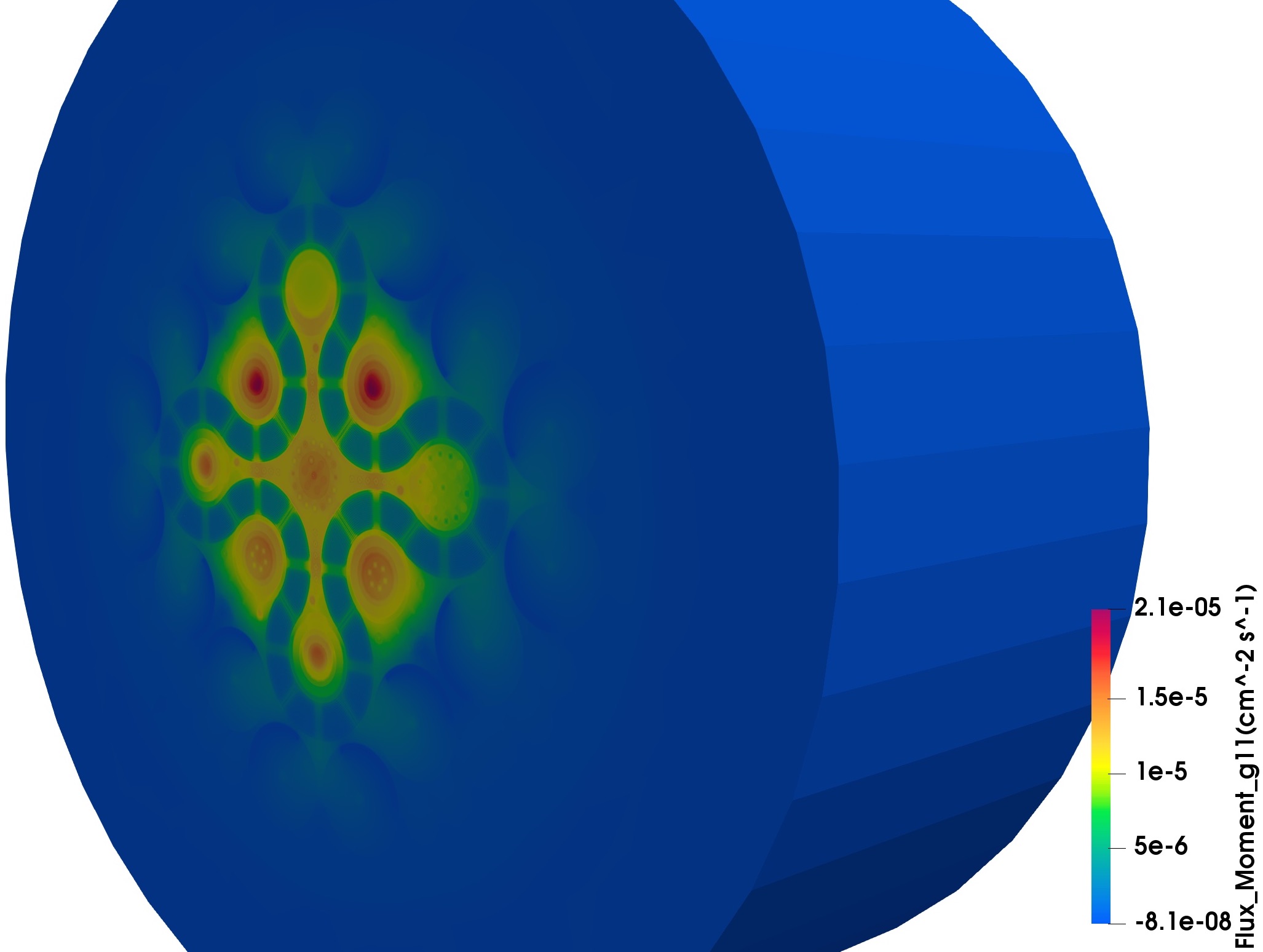
is enfored for the nonlinear solver, and an inexact linear solver with a relative tolerance of $0.5$ is adopted. In the inverse power, one iteration of Newton together with a linear solver with a relative tolerance of $10^{-2}$ is employed. The eigenvalue functions for $1$st, $8$th and $12$th are shown in Fig 3. For convenience, let us define some notations that will be used in the rest of discussions. “$np$” represents the number of processor cores, “NI” is the total number of Newton iterations, “LI” denotes the total number of GMRES iterations, “Newton” is the total compute time spent on the nonlinear solvers and the inverse power iteration, “LSolver” is the compute time on the linear solver, “MF” is the compute time
of the matrix-free operations, “PCSetup” is the compute time of the preconditioner setup, “PCApply” is the compute time of the preconditioner apply, “EFF” is the parallel efficiency, and “NR” is the ratio of the maximum number of mesh nodes to the minimum number of mesh nodes. “LSolver” is part of “Newton”, and it consists of “MF” and the preconditioner. The preconditioner time is split into “PCSetup” and “PCApply”.







Figure 3: Zero-order flux moments for $1$st, $8$th and $12$th groups. 



5.1 Comparison with traditional MASM


We compare the proposed algorithm (denoted as “MASM${}_{\text{sub}}$”) with the traditional MASM. We use a mesh with 4,207,728 elements and 4,352,085 nodes, where, at each node, there are $96$ unknowns consisting of $12$ energy groups and 8 angular directions. That is, the angle is discretized by Level-Symmetric 2 with 8 angular directions. The resulting system of nonlinear equations with 417,800,160 unknowns
is solved using 1,152, 2,304, 4,608, and 8,208 processor cores, respectively. The performance comparison with the traditional MASM is summarized in Table 1 and Fig. 4.


Table 1: Performance comparison with MASM for a problem with 417,800,160 unknowns. The resulting system of nonlinear equations with 417,800,160 unknowns
is solved by an inexact Newton with MASM${}_{\text{sub}}$ and MASM on 1,152, 2,304, 4,608, and 8,208 processor cores, respectively.



$np$
scheme
NI
LI
Newton
LSolver
MF
PCSetup
PCApply
EFF




1,152

MASM${}_{\text{sub}}$

13
191
1855
1701
1418
26
290
100%


1,152
MASM
13
251
2640
2486
1900
162
476
–


2,304

MASM${}_{\text{sub}}$

13
193
989
908
749
21
154
93%


2,304
MASM
13
196
1277
1196
761
155
298
73%


4,608

MASM${}_{\text{sub}}$

13
202
581
535
440
18
90
80%


4,608
MASM
13
194
985
939
426
199
328
47%


8,208

MASM${}_{\text{sub}}$

14
216
404
372
294
22
66
64%


8,208
MASM
13
192
866
835
261
241
343
30%





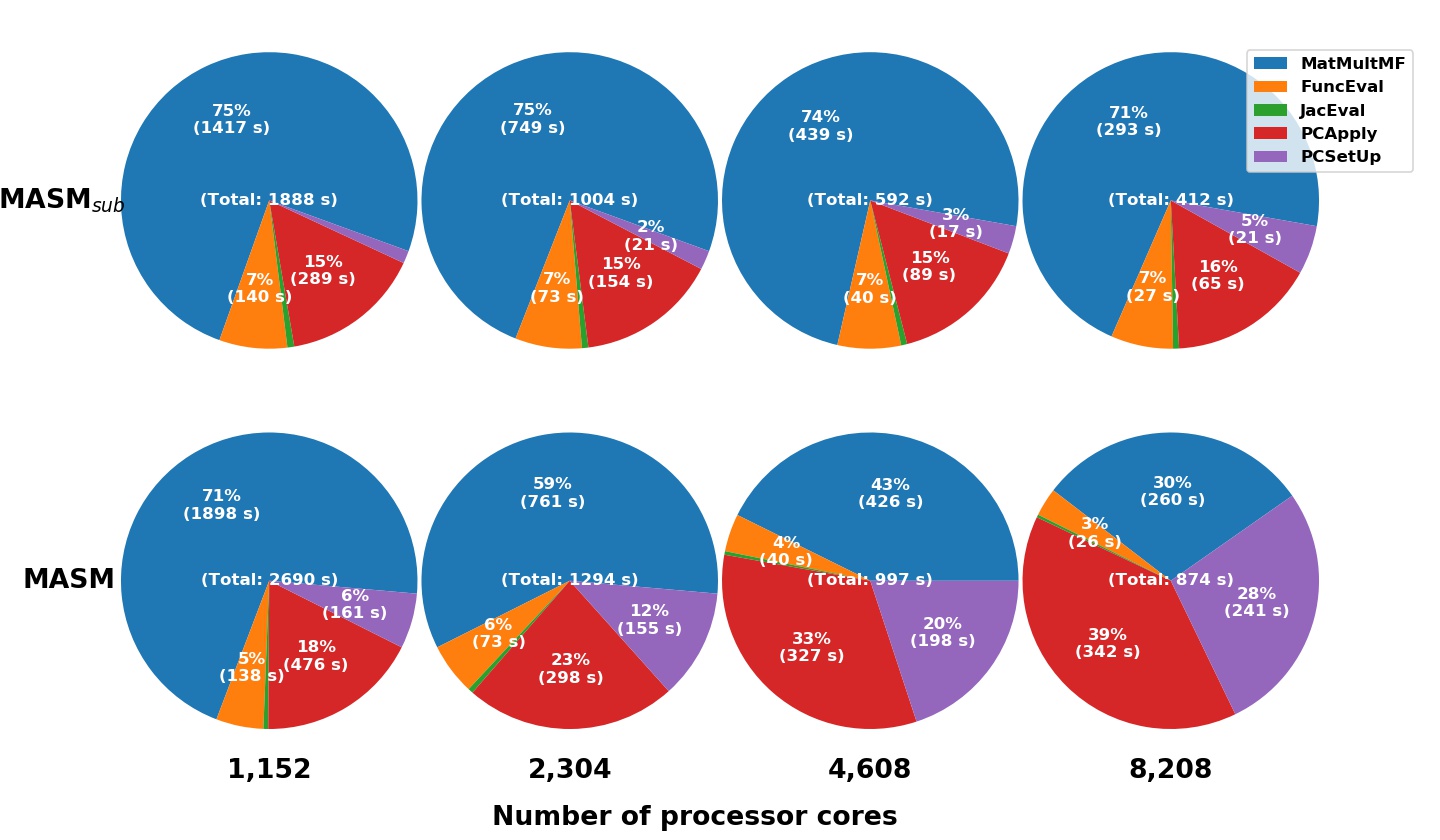
Figure 4: Performance comparison with MASM. The figure shows the compute time spent on Jacobian evaluations (“JacEval”), function evaluations (“FuncEval”), matrix vector multiplications via matrix-free (“MatMultMF”), preconditioner setup (“PCSetUp”) and preconditioner apply (“PCApply”), respectively. 


The nonlinear eigenvalue solver consists of Jacobian evaluation, function evaluation, matrix-vector multiplication, preconditioner setup and preconditioner apply, and where most components except the preconditioner setup are mathematically scalable. As we discussed earlier, the preconditioner setup including the matrix coarsening and the interpolation construction is challenging to parallel, and its compute time sometimes increases significantly when we increase the number of processor cores, which deteriorates the overall algorithm. From Fig. 4, we observed that the preconditioner setup for the traditional MASM is not scalable, and the ratio of the preconditioner setup time to the total compute time is increased significantly when we increase the number of processor cores. The ratio is only $6\%$ when the number of processor cores is $1,152$, but it jumps to $28\%$ when we use $8,208$ processor cores. For the preconditioner setup time, it is $161~{}s$ at $1,152$ cores and increased to $261~{}s$ when $8,208$ processor cores is used. In the traditional MASM, the precodnitioner setup not only is unscalable, but also takes a big chunk of the total compute time so that the overall algorithm performance is deteriorated and the parallel efficiency is reduced to $30\%$ at $8,208$ processor cores. On the other hand, the preconditioner setup of MASM${}_{\text{sub}}$ performs better since it accounts for only $3\%$ ($26~{}s$) of the total compute time at $1,152$ cores and it slightly increases to $6\%$ ($22~{}s$) when we use $8,208$ processor cores. An interesting thing is that the preconditioner setup time of MASM${}_{\text{sub}}$ does not increase much and stays close to a constant. That makes the overall algorithm scale much better, and the parallel efficiency is about $64\%$ even when the number of processor cores is large, i.e., $8,208$. The coarsening algorithm affects not only the preconditioner setup time but also the preconditioner apply time. In the traditional MASM, we observed that the preconditioner apply is not ideally scalable since while it accounts for $16\%$ of the total compute time for $1,152$ processor cores, the ratio is increased to $39\%$ at $8,208$ cores. The corresponding preconditioner apply time is $476~{}s$ for $1,152$ processor cores, and it is decreased to $298~{}s$ by $37~{}s$ when we
double the number of processor cores. Ideally, the preconditioner apply time should be reduced by $50\%$ when the core count is doubled. The preconditioner apply of MASM${}_{\text{sub}}$ is scalable in the sense that the compute time is decreased from $289~{}s$ to $154~{}s$ by $47\%$ when we double the number of processor cores from 1,152 to 2,304, and it is further decreased to $89~{}s$ when we use
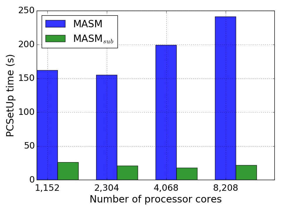
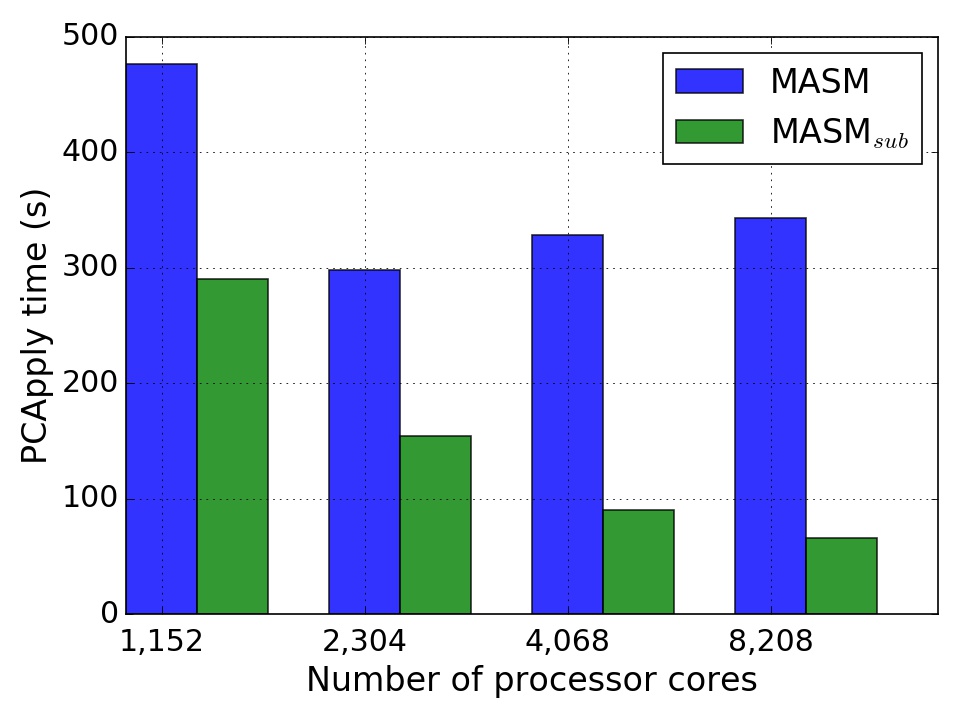
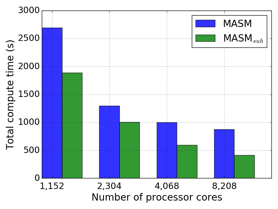
4,608 processor cores. The traditional MASM does not preserve this property, and its preconditioner apply time is actually increased to $327~{}s$ from $298~{}s$ when the core count is doubled from 2,304 to 4,608. The coarsening algorithm based on subspace make MASM${}_{\text{sub}}$ scalable for the ATR simulation while the traditional MASM does not perform well. At 8,208 core, MASM${}_{\text{sub}}$ is twice faster than MASM. These behaviors can be observed from Table 1 as well, where the number of Newton iterations is similar for both MASM and MASM${}_{\text{sub}}$, and the GMRES iteration of MASM${}_{\text{sub}}$ is slightly more than that of MASM at 4,608 and 8,208 cores. The impact of the slight increase of GMRES iteration is negligible since the preconditioner apply per iteration is scalable for MASM${}_{\text{sub}}$. “LSolver” accounts for the most of the overall compute time, and the overall algorithm is scalable as long as the linear solver performs well. The peformance of the linear solver is almost completely determined by the preconditioner since “MF” is well-known to be scalable mathematically. In summary, the eigenvalue solver together with MASM is not scalable, while the MASM${}_{\text{sub}}$ equipped eigenvalue solver performs well since the setup phase of MASM${}_{\text{sub}}$ is optimized and the apply phase of MASM${}_{\text{sub}}$ scales well. The same performance comparison is observed in Fig. 5 as well, where the preconditioner setup of MASM${}_{\text{sub}}$ is almost $10$ times faster than MASM for all processor counts. The preconditioner apply for MASM${}_{\text{sub}}$ is $2$ or $3$ times more efficient than MASM when the number of processor cores is small, and $5$ times faster at 8,208 cores. Due to these behaviors, the overall algorithm based on MASM${}_{\text{sub}}$ is much better than that with MASM. Note that the total compute time in Fig. 4 is slightly more than that in Table 1 since it is calculated by summing up all the individual components that have some overlap.







Figure 5: The compute time comparison on different phases for the problem with 417,800,160 unknowns. Left: preconditioner setup time; middle: preconditioner apply time; right: total compute time. 


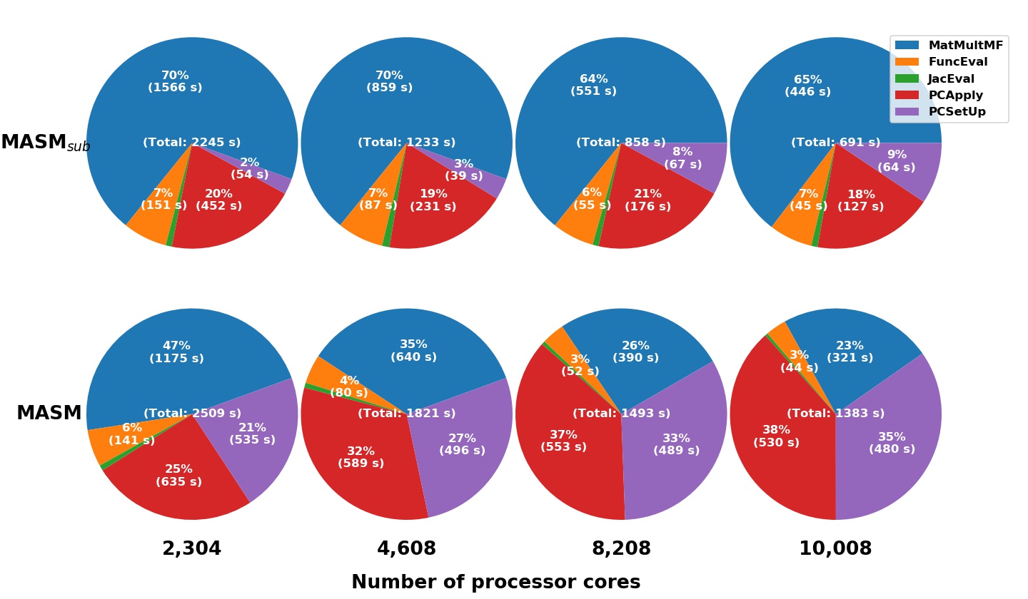
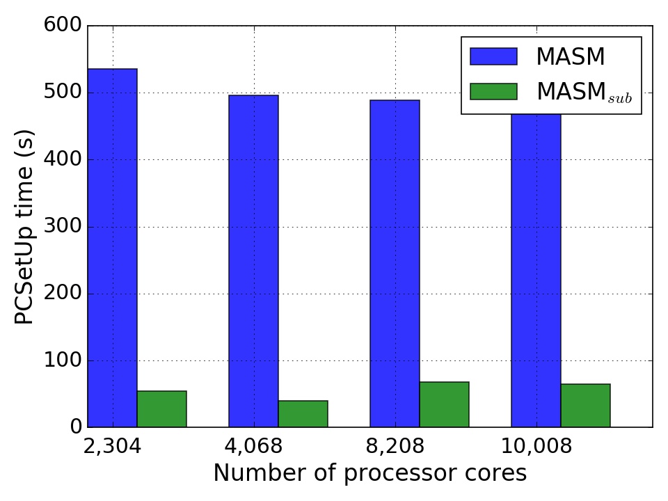
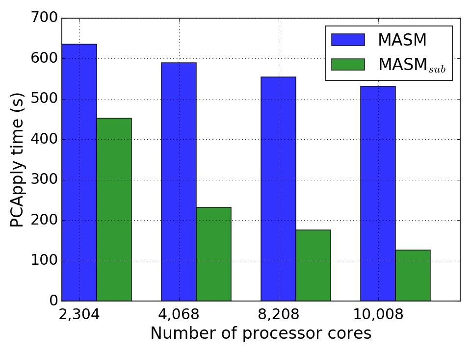
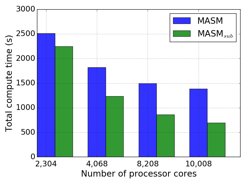
To further verify the effectiveness of the proposed algorithm, we add more angular directions for each mesh node, which leads to 288 variables (24 angular directions $\times$ 12 energy groups) one each mesh node. The same mesh as before is used, but the resulting system is much larger than the previous test, having 1,253,400,480 unknowns, since more angular directions are added for each mesh node. The numerical results are summarized in Table 2, Fig. 6 and 7. In Table 2,
it is easily seen that the number of Newton iterations stays close to a constant as we increase the number of processor cores from 2,304 to 10,008, and the number of GMRES iterations also keeps as
a constant for both MASM and MASM${}_{\text{sub}}$. The number of GMRES iterations for MASM${}_{\text{sub}}$ is more than that obtained via MASM, but the performance of MASM${}_{\text{sub}}$ is not affected much and it is still much better than MASM. The overall algorithm based on MASM${}_{\text{sub}}$ has the parallel efficiency of $76\%$ at 10,008 cores while that for MASM is only $37\%$. Similarly, from Fig. 6 and 7, we observed that the compute time of the preconditioner for MASM${}_{\text{sub}}$ is much smaller than that for MASM.


Table 2: Performance comparison with MASM for a problem with 1,253,400,480 unknowns. The resulting system of nonlinear equations with 1,253,400,480 unknowns
is solved by an inexact Newton with MASM${}_{\text{sub}}$ and MASM on 2,304, 4,608, 8,208, and 10,008 processor cores, respectively. 



$np$
scheme
NI
LI
Newton
LSolver
MF
PCSetup
PCApply
EFF




2,304

MASM${}_{\text{sub}}$

13
191
2202
2027
1566
54
452
100%


2,304
MASM
12
147
2466
2302
1176
535
635
–


4,608

MASM${}_{\text{sub}}$

13
183
1199
1096
860
41
232
92%


 4,608
MASM
12
139
1791
1694
641
496
589
61%


8,208

MASM${}_{\text{sub}}$

13
183
828
763
552
68
176
75%


8,208
MASM
12
135
1474
1412
391
489
554
42%


10,008

MASM${}_{\text{sub}}$

14
184
672
617
447
65
127
76%


10,008
MASM
12
134
1369
1317
322
480
531
37%





Figure 6: Performance comparison with MASM for the problem with 1,253,400,480 unknowns. The figure shows the compute time spent on Jacobian evaluations (“JacEval”), function evaluations (“FuncEval”), matrix vector multiplications via matrix-free (“MatMultMF”), preconditioner setup (“PCSetUp”) and preconditioner apply (“PCApply”), respectively. 







Figure 7: The compute time comparison on different phases for the problem with 1,253,400,480 unknowns. Left: preconditioner setup time; middle: preconditioner apply time; right: total compute time. 




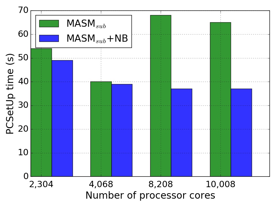
5.2 Node balance improvement


Typically, before a finite element simulation starts, a dual graph of mesh (where each graph vertex corresponds to a mesh element) is partitioned into $np$ submeshes that have nearly equal number of elements. While the number of elements assigned to each processor core is nearly equivalent, some processor cores may have more mesh nodes since the shared mesh nodes along the processor boundaries are simply assigned to the cores with lower MPI rank. A scalable calculation requires to balance both mesh elements and mesh nodes. We use a partition-based node assignment, as discussed in our previous work [18], to balance the overall calculation. The basic idea of the partition-based node assignment is that the processor boundary mesh is partitioned
into two parts, and each part is assigned to a processor core who shares the processor boundary mesh with the other processor core. Interested readers are referred to [18] for more details. The same configuration as before is used, and the numerical results are shown in Table 3 and 4, and Fig. 8.


Table 3: Mesh node assignment for the problems with 417,800,160 unknowns. 



$np$
scheme
NI
LI
Newton
LSolver
MF
PCSetup
PCApply
EFF




1,152

MASM${}_{\text{sub}}$

13
191
1855
1701
1418
26
290
–


1,152

MASM${}_{\text{sub}}$+NB

13
199
1821
1674
1407
26
270
100%


2,304

MASM${}_{\text{sub}}$

13
193
989
908
749
21
154
92%


2,304

MASM${}_{\text{sub}}$+NB

13
207
1005
928
769
19
158
91%


4,608

MASM${}_{\text{sub}}$

13
202
581
535
440
18
90
78%


4,608

MASM${}_{\text{sub}}$+NB

13
216
579
534
436
18
89
79%


8,208

MASM${}_{\text{sub}}$

14
216
404
372
294
22
66
63%


8,208

MASM${}_{\text{sub}}$+NB

14
217
379
348
272
21
62
67%





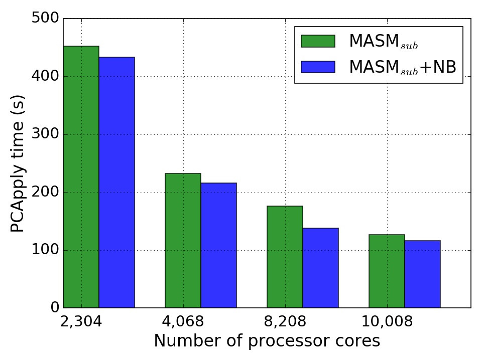
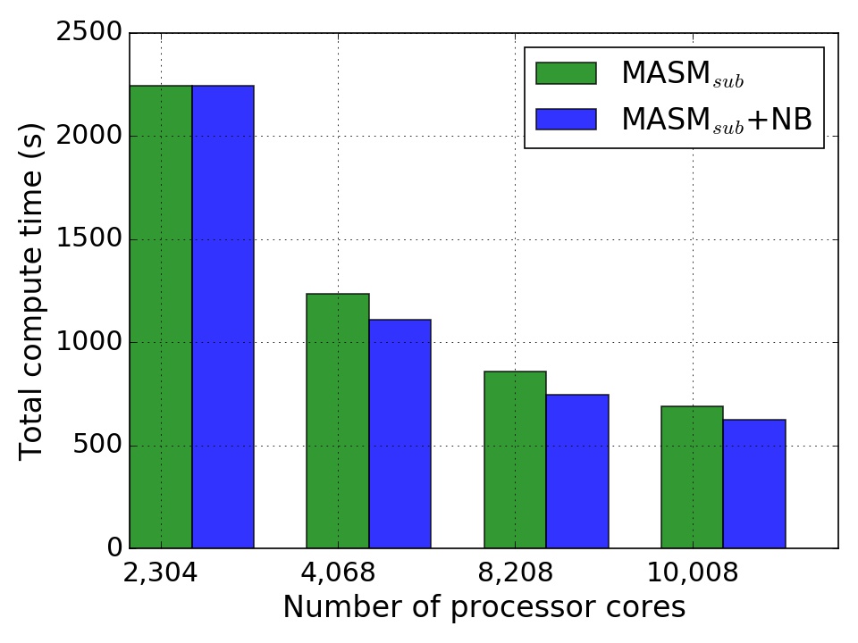
From Table 3, we observed that the compute time for different components is further improved using the node assignment strategy. The improvement becomes more obvious when the number of variables for each mesh node is increased. In Table 4, the preconditioner setup time is significantly reduced, for example, it is reduced to $37~{}s$
from $65~{}s$ at 10,008 processor cores, which leads to the parallel efficiency increased from $76\%$ from $83\%$. The same observation is found in Fig. 8 as well.


Table 4: Node assignment for the problem with with 1,253,400,480 unknowns.



$np$
scheme
NI
LI
Newton
LSolver
MF
PCSetup
PCApply
EFF




2,304

MASM${}_{\text{sub}}$

13
191
2202
2027
1566
54
452
100%


2,304

MASM${}_{\text{sub}}$+ NB

13
191
2203
2018
1575
49
433
–


4,608

MASM${}_{\text{sub}}$

13
183
1199
1096
860
41
232
92%


4,608

MASM${}_{\text{sub}}$+NB

13
185
1093
1001
766
39
216
100%


8,208

MASM${}_{\text{sub}}$

13
183
828
763
552
68
176
75%


8,208

MASM${}_{\text{sub}}$+NB

13
189
732
670
511
37
138
84%


10,008

MASM${}_{\text{sub}}$

13
184
672
617
447
65
127
76%


10,008

MASM${}_{\text{sub}}$+NB

13
187
610
557
420
37
116
83%










Figure 8: The compute time comparison on different phases for the problem with 1,253,400,480 unknowns using a node balancing strategy. Left: preconditioner setup time; middle: preconditioner apply time; right: total compute time. 




5.3 Aggressive coarsening


The numerical results shown earlier are obtained using 10 levels of aggressive coarsening. The aggressive coarsening, Alg. 6, is used to reduce the complexities of the operators and the interpolations. More levels are applied by the aggressive coarsening, and the complexities of the operators and the interpolations become lower, but at the same time the convergence may be deteriorated. In this test, different numbers of levels of aggressive coarsening are applied in MASM${}_{\text{sub}}$, and the results are summarized in Table 5, where “Agg” denotes the number of levels of aggressive coarsening, and “Agg=0” corresponds to no aggressive coarsening.


Table 5: Different number of aggressive coarsening levels for the problems with 417,800,160 unknowns. “Agg” denotes the number of aggressive coarsening levels. 



$np$
Agg
NI
LI
Newton
LSolver
MF
PCSetup
PCApply
EFF




1,152
0
13
209
2242
2088
1853
55
509
100%


1,152
2
14
210
2068
1906
1570
33
347
–


1,152
4
13
206
2007
1853
1542
26
322
–


1,152
10
13
191
1855
1701
1418
26
290
–


2,304
0
13
208
1199
1118
820
45
278
77%


2,304
2
13
195
1027
945
758
25
178
90%


2,304
4
13
206
1059
978
801
20
174
88%


2,304
10
13
193
989
908
749
21
154
94%


4,608
0
13
206
677
632
457
34
160
68%


4,608
2
13
199
591
546
423
21
113
78%


4,608
4
13
210
606
558
449
18
104
80%


4,608
10
13
202
581
534
440
18
90
94%


8,208
0
14
217
490
457
302
46
123
53%


8,208
2
13
204
412
379
277
25
87
63%


8,208
4
13
200
385
355
273
21
70
68%


8,208
10
14
216
404
372
294
22
66
64%





From Table 5, we observed that both Newton iteration and GMRES iteration do not change much when we apply different numbers of levels of the aggressive coarsening in MASM${}_{\text{sub}}$. The preconditioner time including the setup and apply is reduced significantly when the number of levels of of aggressive coarsening is increased from 0 to 2, and then it slightly decreases when we increase “Agg” from 2, 4 to 10. For example, in 8,208-core case, the preconditioner apply time is decreased from $123~{}s$ to $87~{}s$ when “Agg” is increased from 0 to 2, and it
is reduced to $70~{}s$ and $66~{}s$ when “Agg” is 4 and 8. Due to these factors, the corresponding parallel efficiency is increased from $53\%$ to $64\%$ when the number of levels of aggressive coarsening is increased from 0 to 10. It is the reason why we have used 10 levels of aggressive coarsening in our previous tests.




5.4 Strong scalability


In this test, we study the strong scalability using a “fine” mesh with 25,856,505 nodes and 26,298,300 elements. The resulting eigenvalue system of equations with 2,482,224,480 unknowns is solved by an inexact Newton preconditioned by MASM${}_{\text{sub}}$. At the beginning of the strong scaling study, we also test the impact of the number of levels of aggressive coarsening on the overall algorithm for the “fine” mesh case. 4 and 10 levels of aggressive coarsening are tested, and the results are summarized in Table 6. The case with 10 levels of aggressive coarsening has slightly better results than that obtained with “Agg=4”.


Table 6: Different number of aggressive coarsening levels for the problem with 2,482,224,480 unknowns. 



$np$
Agg
NI
LI
Newton
LSolver
MF
PCSetup
PCApply
EFF




4,608
4
12
161
2596
2369
1853
114
457
100%


4,608
10
13
171
2808
2567
2002
131
511
–


6,048
4
13
170
2125
1939
1499
95
391
93%


6,048
10
13
171
2084
1898
1510
84
352
95%


8,208
4
12
160
1749
1613
1134
150
404
83%


8,208
10
12
161
1707
1570
1139
142
364
85%


10,008
4
12
161
1459
1343
949
141
308
82%


10,008
10
12
160
1423
1307
951
138
274
84%





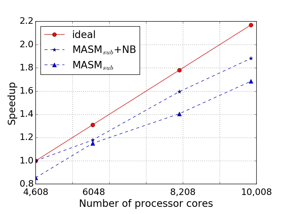
We therefore use 10 levels of aggressive coarsening in the following scaling study. The numerical results are shown in Table 7. The performance of the node balancing strategy is also reported, and the corresponding algorithm is denoted as “MASM${}_{\text{sub}}$+NB”. Again, for MASM${}_{\text{sub}}$, the numbers of Newton iterations and GMRES iterations stay as constants when we increase the number of processor cores, which indicates that the algorithm is mathematically scalable. The total compute time (“Newton”) is decreased proportionally when
we increase the number of processor cores from 4,608 to 10,008. For instance, the total compute is reduced from $2808~{}s$ to $2084~{}s$, when we increase the number of processor cores from
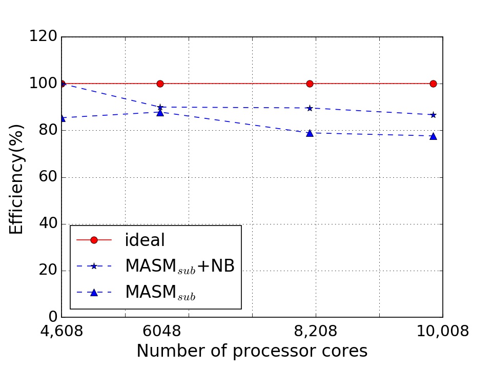
4,608 to 6,048, and it further is reduced to $1707~{}s$ and $1423~{}s$ when the number of processor cores is 8,208 and 10,008. The preconditoner setup is not scalable, but it does not affect the overall performance much since it accounts for only a small portion of the total compute time. A good parallel efficiency of $77\%$ is achieved at 10,008. While the performance of MASM${}_{\text{sub}}$ is already good, it can be further enhanced by applying the node balancing strategy to make the overall distribution more balanced. In the odd rows of Table 7,
the node balancing strategy is able to improve the overall algorithm performance, especially, the preconditioner setup time is significantly reduced. For example, at 8,208 cores, the compute time is reduced by $200~{}s$ when the node balancing strategy is used, most of the time reduction results from the improvement of the preconditioner setup. At 10,008 cores, the preconditioner setup time is
reduced to $82~{}s$ from $138~{}s$. The preconditioner apply also benefits from a more balanced workload, for example, the preconditioner apply time is reduced from $274~{}s$ to $208~{}s$ at 10,008
processor cores. We have almost-perfect parallel efficiencies when we use MASM${}_{\text{sub}}$+NB. The parallel efficiency is as high as $87\%$, even when the number of processor cores is more than 10,000. The Schwarz preconditioner together with both the subspace-based coarsening and the partition-based node balancing offers a highly scalable solver for the eigenvalue calculations for the targeting application. The corresponding parallel efficiency and speedup are plotted in Fig. 9.


Table 7:  Strong scalability with a “fine” mesh with 25,856,505 nodes, 26,298,300 elements, and 2,482,224,480 unknowns. 



$np$
Scheme
NI
LI
Newton
LSolver
MF
PCSetup
PCApply
NR
EFF




4,608

MASM${}_{\text{sub}}$+NB

12
160
2398
2182
1743
94
396
1.8
100%


4,608

MASM${}_{\text{sub}}$

13
171
2808
2567
2002
131
511
2.2
–


6,048

MASM${}_{\text{sub}}$+NB

13
176
2035
1858
1470
87
337
1.8
90%


6,048

MASM${}_{\text{sub}}$

13
171
2084
1898
1510
84
352
2.7
89%


8,208

MASM${}_{\text{sub}}$+NB

12
167
1504
1373
1081
76
244
2
90%


8,208

MASMsub

12
161
1707
1570
1139
142
364
2.8
79%


10,008

MASM${}_{\text{sub}}$+NB

13
168
1275
1160
896
82
208
2
87%


10,008

MASMsub

12
160
1423
1307
951
138
274
2.9
77%









Figure 9: Parallel efficiency and speedup for the problem with 2,482,224,480 unknowns. Left: speedup, right: parallel efficiency. 



6 Conclusions


A parallel Newton-Kyrlov-Schwarz method is studied for the numerical simulation of the multigroup neutron transport equations on 3D unstructured spatial meshes. A hierarchal partitioning is used to divide the computational domain into a large number of subdomains while the existing partitioners are from ideal. Two novel components including the subspace-based coarsening and the partition-based workload balancing are introduced and carefully studied. The total compute time using the subspace-based coarsening is halved compared with the traditional approach, and therefore the corresponding parallel efficiency is doubled to $76\%$ when more than 10,000 processor cores are used. In addition, the partition-based workload balancing is able to assign a nearly equal amount of work to each processor core, and the parallel efficiency at 10,000 is further increased to $87\%$. The scalability of the overall algorithm is studied for a realistic application with 2,482,224,480 unknowns on a supercomputer with up to 10,008 processor cores.


While this paper focuses on the multilevel Schwarz preconditioner, other popular methods such as DSA [1] and NDA (nonlinear diffusion acceleration method) [25] will be explored in the future.